Article

Two Ways to Quantify Korean Drought Frequency: Partial Duration Series and Bivariate Exponential Distribution, and Application to Climate Change

1
Division of Earth Environmental System Science (Major of Environmental Engineering), Pukyong National University, Busan 48513, Korea
2
Department of Environmental Engineering, Pukyong National University, Busan 48513, Korea
3
Department of Aeronautics and Civil Engineering, Hanseo University, Seosan 31962, Korea
*
Author to whom correspondence should be addressed.
Atmosphere 2020, 11(5), 476; https://doi.org/10.3390/atmos11050476
Submission received: 14 April 2020 / Revised: 1 May 2020 / Accepted: 4 May 2020 / Published: 7 May 2020
(This article belongs to the Special Issue Meteorological Extremes in Korea: Prediction, Assessment, and Impact)

Abstract

:
Studies using drought index to examine return levels of drought can be classified into two approaches: univariate frequency analysis using annual series extracted from drought index time series and multivariate frequency analysis that simultaneously reflects various characteristics of drought. In the case of drought analysis, it is important to properly consider the duration, so, in this study, univariate frequency analysis is performed using the partial duration series. In addition, a bivariate frequency analysis is performed using a relatively simple bivariate exponential distribution to give a more realistic return level to major drought events in the past while reflecting the correlation between drought severities and durations. The drought severity–duration–frequency curves using each of the two frequency analyses are derived, and these curves are used to examine how the drought phenomenon currently in progress is evolving. From this, the advantages and disadvantages of the two approaches, as well as the points to be aware of in application, are discussed. Finally, using the two approaches to the proposed drought frequency analysis, the behavior of Korea’s future extreme droughts is investigated under the conditions of various future climate change scenarios.

1. Introduction

Unlike flooding, drought is difficult to quantify since it occurs over a large area over a relatively long period of time. Even if one wants to look at the characteristics of a drought at a particular site, various characterizations should be involved: identification of drought events including the start and end times of drought, the duration of drought events, the cumulative or averaged drought severity during the duration of the drought, and many others. Therefore, it is very difficult to quantify drought by reflecting them properly. The most common method of quantifying drought is to use a drought index. Various drought indices have been developed by using factors such as precipitation, evapotranspiration, soil moisture, reservoir storage, and river flow rate in accordance with the purpose of use [1].
Studies examining the return level of drought from the drought index can be broadly classified into two approaches. The first is an approach that extracts an annual maximum (or minimum) series (AMS) from the drought index time series and analyzes the univariate frequency. The second is an approach that performs multivariate frequency analysis by simultaneously reflecting various characteristics of drought events [2]. Yoo and Kim [3] derived SDF (drought severity-duration-frequency) curves using the method of applying SPI (standardized precipitation index, [4]) to the Poisson rectangular plus point rainfall model under the assumption that drought severity and duration are independent of each other. Then, Kim and Yoo [5] analyzed the spatial distribution characteristics of drought severity in Korea using the method proposed by Yoo and Kim [3]. A variety of previous studies using univariate frequency analysis can be found worldwide. Ghosh and Mujumdar [6] projected India’s future 10-year drought using a 12-month time scale SPI. Lehner et al. [7] suggested a drought severity corresponding to a return level of 100-year using the log-Pearson type 3 distribution. Mishra and Singh [8] performed frequency analysis using the Gumbel distribution from the SPI time series. Vidal and Wade [9] studied changes in the future drought severity using SPIs of various time scales. Lee and Kim [10] derived SDF curves by extracting drought severity AMS for various durations and then performing frequency analysis for each duration. Kang and Moon [11] derived SDF curves in the northern part of the Korean Peninsula in a similar way. Kim et al. [12] analyzed changes in the future drought severity through frequency analysis of the SPI time series, and Park et al. [13] and Kim et al. [14] also examined the future extreme drought using SDF curves derived from SPI’s AMS for various durations. In the above studies, the relationship between drought severity and duration was not specifically treated since the relationship between drought severity and duration was assumed independently, or AMS extracted using different durations were independently analyzed. However, in the above studies, the method of extracting the AMS required to perform the frequency analysis was not clearly described, or in some studies, the method of mechanically extracting the AMS based on the year was taken. Since drought events occur at any time of the year and sometimes occur for a long period of time through several years, the accuracy of frequency analysis depends largely on how AMS for frequency analysis is extracted [15].
In the case of multivariate drought frequency analysis, in particular, quantification of drought using drought severity and duration has been actively conducted. To analyze the two-dimensional probability behavior between drought severity and duration, it is necessary to estimate the joint probability distribution between drought severity and duration, and various studies have been conducted on this [16]. Dalezios et al. [17] performed a drought frequency analysis using the PDSI (Palmer drought severity index, [18]) for the Greek region and analyzed the SDF relationship between the drought period and the wet period. Shiau and Shen [19] attempted to quantify the risk of drought in the study basin by performing a risk analysis for the drought severity using a conditional copula model and then estimating the drought severity for a specific duration. In addition, Shiau [20] applied various two-variable copula for drought severity and duration and performed frequency analysis using a joint distribution and conditional distribution for each copula function. Yeon et al. [21] estimated the return level for major drought events in the past after deriving the joint probability density function between drought severity and duration for the case where the marginal distribution of drought duration and conditional distribution of drought severity were given. Shiau and Modarres [22] attempted to determine the drought situation in the unmeasured basin by developing SDF curves from the drought severity and duration data based on the copula function. Ganguli and Reddy [23] also estimated the risk of drought using conditional return levels, and Mirabbasi et al. [24] constructed an optimal copula model for the severity and duration of the drought through error analysis and the analysis of the dependency of the tail and performed a bivariate drought frequency analysis. Chen et al. [25] performed multivariate frequency analysis by applying the minimum value of the drought index and the time of drought to the copula function as well as the drought severity and duration, and Halwatura et al. [26] used SDF curves to investigate the applicability of rapid drought situation determination and probability drought mapping. Chun et al. [27] analyzed the frequency of drought using the hidden Markov chain model and the bivariate (drought severity and duration) copula function, and Kim et al. [28] performed drought frequency analysis using a trivariate copula function including cumulative drought severity in addition to the average drought severity and duration. In addition, since the three-dimensional shape of the bivariate joint distribution using the copula function decreases practical intuition, Yu et al. [29] calculated the conditional probability distribution function for each duration from the copula function and proposed the concept of threshold drought severity for non-excess probability. Kwon et al. [30] also performed bivariate drought frequency analysis using the copula function for SPI and precipitation deficit. In most studies, bivariate frequency analysis was performed using drought severity and duration, and it can be seen that copula functions are generally used to estimate the probability distribution. This is because the copula function can well reflect the correlation between hydrological variables [31]. However, in order to use the copula function, a number of drought events sample data representing various drought severities and various durations observed over a relatively long period of time should be secured. Therefore, when the number of drought events used in the analysis is only a few tens, it is difficult to secure the reliability of the result. In particular, SDF curves derived by using the copula function from drought events that occurred during observation periods of less than 40 years were found to estimate the return level of major drought events in the past, going back at least 200 years and up to 5000 years or more.
In this study, we tried to quantify the frequency of drought using two approaches: univariate frequency analysis and bivariate frequency analysis. In the case of univariate frequency analysis, partial duration series (PDS) for each duration was extracted from the SPI time series using the method proposed by Stall [32], which is applied to the low flow rate analysis of reservoir inflow. In the case of the bivariate frequency analysis, in order to reflect the correlation between the drought severity and the duration and, at the same time, to give a more realistic return level to the major drought events in the past, the joint probability density function between drought severity and duration was constructed using a relatively simple bivariate exponential distribution. The temporal behavior of past drought events was examined using SDF curves derived from two approaches. We also investigated whether the induced SDF curves can be used as a tool to quantitatively recognize the progress of drought when a drought event occurs. From this, the advantages and disadvantages of applying the two approaches and the considerations to be taken in application were discussed. Finally, the behavior of future extreme droughts was analyzed under the conditions of future climate change scenarios using two quantification methods of drought frequency analysis.

2. Methods

2.1. Data

The data used in this study are monthly precipitation data from the Daeghwanryeong site, Mokpo site, Namhae site, and Seosan site operated by the KMA (Korea Meteorological Administration). The data period of selected sites is 38 years from 1981 to 2018, and the SPI time series with a 6-month time scale for 37 years from 1982 to 2018 was analyzed. The locations of the four sites applied are shown in Figure 1.
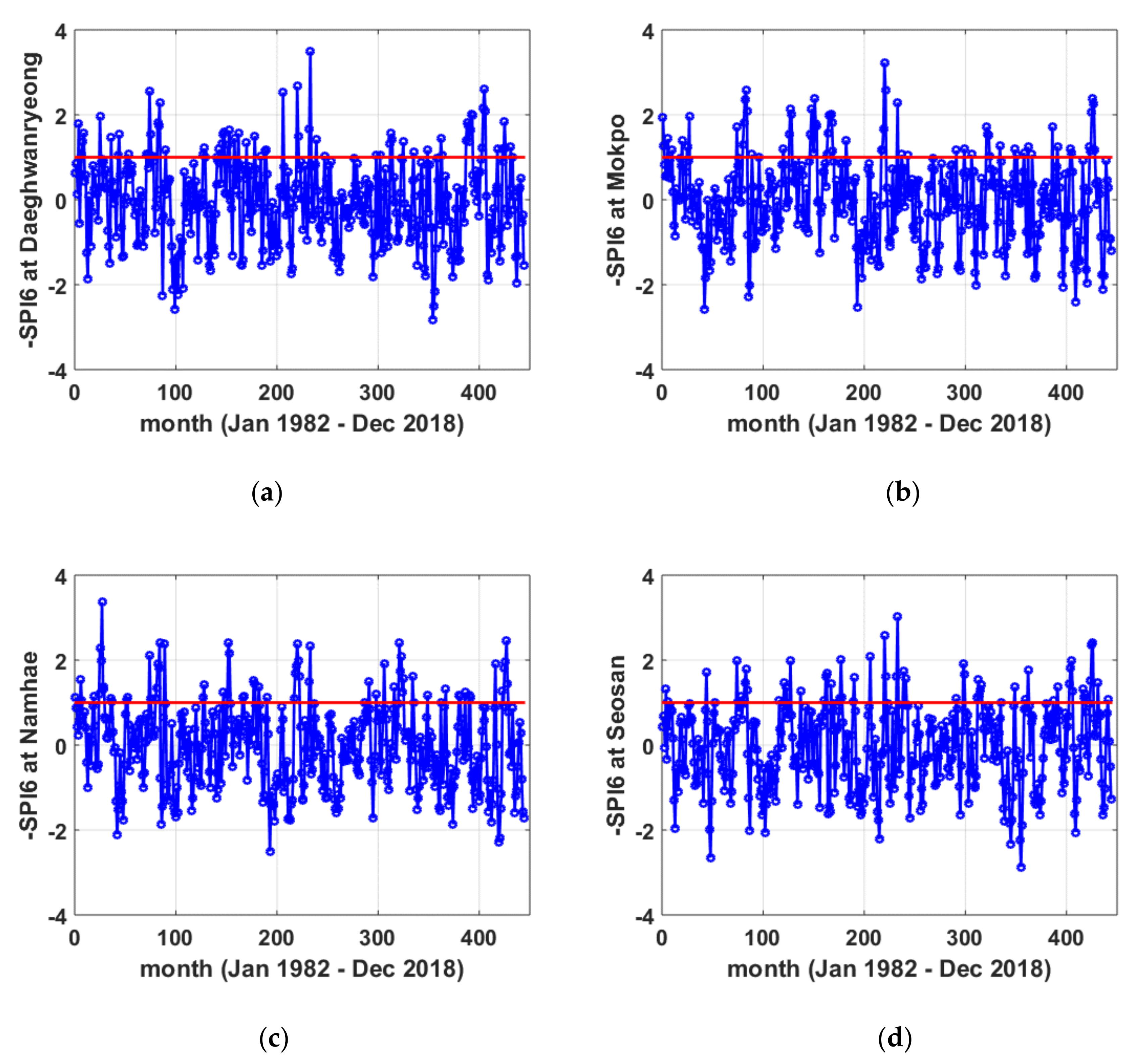
In this study, SPI was applied as the drought index. SPI is one of the most widely used drought indices, due to its simple calculation procedure using only precipitation and its advantages for reflecting regional characteristics [33]. SPI is derived from the probability distribution function, which explains precipitation data well. The value of SPI is quantified to the extent that the observed precipitation deviates from the long-term average. Among the SPIs of various time scales, a 6-month time scale SPI that superimposes the attributes of short-term and long-term drought was used for analysis. In Korea, rainfall is mainly concentrated in the summer months, and rain during this period affects the spring of the following year, so cumulative rainfall over a period of six months, which is relatively long compared to other countries, is used for drought management [10]. KMA’s drought warning is also performed using a 6-month time scale SPI. The probability distribution for SPI calculation was applied to the two-parameter Gamma distribution used as a standard in Korea [34], and the parameters were estimated by the L-moment method [35]. Figure 2 shows the SPI time series at selected sites. Since the drought is a negative SPI, the sign of the SPI is changed for frequency analysis to convert the positive to a drought.
Figure 2 shows representative past drought events that occurred in Korea in 1984, 1988, 1994–1995, 2000, 2001, 2014–2015, and 2017. Even relatively recently, it can be found that Korea has experienced drought.

2.2. Partial Duration Series

For univariate frequency analysis, AMS should be extracted from monthly SPI time series. When estimating design rainfall depth using the block maxima approach, AMS for each duration is extracted from rainfall data. However, in the case of drought analysis, it is very important to properly consider the duration, so the extraction of AMS is not simple. In this study, the PDS for each duration was extracted from the SPI time series by the following procedure using the method proposed by Stall [32], which is applied to the low flow rate analysis of the reservoir inflow:
  • Obtain a moving average time series, B , for each duration from the monthly SPI time series, A .
  • The smallest sample in time series B is selected first, and the selected sample is deleted. Then, the sample series as many as the number of months of the duration before and after the deleted sample is deleted to form a time series C .
  • The smallest sample among time series C is selected as the second rank, and the selected sample is deleted. Then, samples as many as the number of months in the duration before and after the deleted sample are deleted to form a new time series D .
  • Create a PDS by repeating this procedure and selecting the smallest samples.
The number of PDS samples cannot exceed the observed number of years, and if the value of the selected sample is greater than zero, the iterative process is stopped. Therefore, the maximum number of PDS samples will be the number of years observed, and if the duration is long, the number of samples may be less than the number of years observed. When estimating the return level of drought severity, the number of PDS samples should be considered. The return level of drought severity s and duration d of PDS can be estimated as follows:
T r s , d = 1 λ 1 F s
where λ is the probability of occurrence of PDS, that is, the number of PDS samples divided by the number of years observed, and F s is the cumulative probability distribution of the drought severity. In this study, F s was applied to the Gumbel distribution whose parameters were estimated by the L-moment method.

2.3. Drought Events

Unlike univariate analysis, it is necessary to define drought events for bivariate analysis. In this study, using the Run theory proposed by Yevjevich [36], the drought event was defined as a period in which the SPI drought criterion of −1 or less was continuous (see Figure 3). That is, the duration D of the drought event means a period in which the SPI below the threshold level is −1. Drought severity denoted by S is the mean value of SPI within the drought duration D . For convenience, drought severity S is taken to be positive, which is defined by:
S = 1 D i = 1 D S P I i S t h ,
where S t h is −1, the threshold level of drought.

2.4. Bivariate Exponential Distribution

For the development of SDF curves considering the correlation between drought severity and duration, the joint probability distribution function (PDF) given by Nagao and Kadoya [37] is employed in this study. Of several types of bivariate exponential distributions that can be found in extensive literature reviews, the Nagao–Kadoya distribution has a general form with marginals that are standard exponential distributions and the correlation coefficient not posing any restrictions on the cross-correlation coefficient [38]. The joint PDF is as follows:
f S , D s , d = β δ 1 ρ exp β s δ d 1 ρ × I o 2 ρ β δ s d 1 / 2 1 ρ
where s is the mean severity of drought event, d is the duration of drought event, β is the reciprocal of the expected value of s , δ is the reciprocal of the expected value of d , ρ is the cross-correlation coefficient of s and d , and the function I o () is the Bessel function of the first kind with the order zero. The PDF introduced by Nagao and Kadoya [37] in Equation (3) was used by Cordova and Rodriguez-Iturbe [39] and Goel et al. [40] in their study of the probabilistic structure of storm surface runoff to account for correlation between rainfall intensity and duration. Ashkar et al. [41] also used this PDF to investigate the relation of the volume and duration of low-flow events in river channels to manage water resources and design hydraulic structures.
The joint return period T r s , d of the drought event s , d can be defined as follows:
T r s , d = 1 λ 1 F s , d
where F s , d is the conditional non-exceedance probability when a drought event occurs, and can be defined as F s , d = Pr S s   o r   D d , and λ is the probability of a drought event occurring in a certain year. Equation (4) represents the return level when either s or d or both are exceeded ( S > s , or D > d , or S > s and D > d ). In the univariate frequency analysis, the return level can be estimated using the non-exceedance probability. However, since the drought event is expressed by the mean drought severity and the duration in the bivariate frequency analysis, an estimation method of the return level which considers both variables simultaneously is required. Hence, the joint return level of the drought event ( S > s & D > d , i.e., both s and d are exceeded) can be defined as follows:
T r e s , d = 1 F e s , d
where F e s , d is the exceedance probability, and is defined as follows:
F e s , d = λ × Pr S > s   &   D > d = λ s d f S , D s , d d d ds

3. Results

3.1. Frequency Analysis Using Partial Duration Series

Table 1 shows the number of PDS samples corresponding to each duration derived using the method proposed by Stall [32]. Up to a 5-month duration, PDS consisting of 37 samples equal to the number of data years could be constructed, but the longer the duration, the smaller the number of PDS samples. This is because, when creating a PDS, samples located before and after the sample selected as a member of the PDS are removed to secure independence between the PDS samples. The number of samples of a 12-month duration PDS at the Mokpo site is 16, which is the smallest number of PDS samples applied. The probability of the occurrence of drought (i.e., λ of Equation (1)) for a duration of 12 months at the Mokpo site is 16/37 = 0.4324, which is the number of PDS samples divided by the number of years observed. The site with the largest number of PDS samples for a 12-month duration is Daeghwanryeong, and the corresponding λ is 21/37 = 0.5676. The PDSs from the four sites are shown in Figure S1.
Table 2 shows the times when the most severe drought occurred for a specific duration. With a short duration of less than 2 months at Daeghwanryeong site, it was found that the drought was the most severe in the spring of 2001, but, overall, the most severe drought occurred in 2014–2015. At the Mokpo site, the drought was the most severe in the spring of 2000 for short durations of less than 3 months, and the drought was the most severe in 1994–1995 for the longer durations. Drought at the Namhae site was the most severe in 1984, and drought in 1988 and 2017 was the most severe at the Seosan site. Korea has a relatively small land area, but as can be seen from the results of the above four sites, it can be found that the spatial variability of drought is very large. Looking at these results from a different point of view, it can be said that the so-called mega-drought event that swept the whole country has not yet occurred.
The result of fitting a 3-month duration PDS to the Gumbel distribution can be seen in Figure S2. It can be seen that some PDSs follow the Gumbel distribution very well (see Figure S2a,d), while others do not (see Figure S2b,c). However, the results of the goodness-of-fit test showed that it is possible to apply the Gumbel distribution to most PDSs.
Figure 4 shows the SDF curves derived using PDS. It can be recognized that the drought index observed to be the most severe for a specific duration generally corresponds to the SDF curves corresponding to the return levels between 20 years and 50 years, and the drought index observed as the seventh most severely coincides with the SDF curve corresponding to the 5-year return level. The observed drought indices in other rankings also showed good agreement with the SDF curves for the corresponding return level. This means that the method of this study that makes SDF curves using PDS and Gumbel distributions is reasonable.

3.2. Frequency Analysis Using Bivariate Exponential Distribution

Table 3 shows the statistics of drought events estimated at four sites. During the 37 years, an average of 35 drought events occurred (average of four sites), and there are slight differences among sites. The average of drought severity S defined in Equation (2) was found to be 0.41 to 0.46, and the average of duration D was about 2 months. In other words, the statistics of the analyzed sites indicate that a drought event occurs every 11 to 14 months in Korea, and the average drought severity when a drought event occurs is 0.44 on average and lasts for 1.9 months. On the other hand, since the difference between the mean and standard deviation of the drought severity is not significantly different, it can be seen that it is reasonable to fit the drought severity to the exponential distribution. Likewise, it would be possible to adapt the duration of drought to the exponential distribution.
Table 4 shows the drought event with the most severe drought severity and the longest drought duration. The duration of drought events with the most severe drought severity was mainly selected between 1 month and 2 months. Since the drought severity is an average value for the duration of the drought event, the longer the drought duration, the smaller the drought depth is. The average SPI for drought events with the most severe drought severity is −2.33. In the concept of non-exceedance probability, such a value can be regarded as a very severe rainfall shortage of more than 99 %. Except for the Namhae site, it was spring of 2001 that recorded the most severe drought severity. In fact, in the spring of 2001, rice planting was not carried out on time due to drought, causing severe agricultural damage [1]. For reference, the return level in Table 4 is the result of univariate frequency analysis.
The longest drought duration ranged from 5 months to 7 months. The average SPI for drought events corresponding to the longest duration of drought is −1.67. In the concept of non-exceedance probability, this value is more than 95%. This means that the period of insufficient rainfall, which is less than 5% of the occurrence probability, continued for 5 to 7 months. The time of occurrence of drought events that caused the maximum drought severity was concentrated in the spring of 2001, but the time of occurrence of drought events that persisted for the maximum duration varied from site to site. The cause can be found in the climate characteristics of the Korean Peninsula. In other words, in the case of the Korean Peninsula, localized heavy rains occur within a period of 5 to 7 months, and droughts are (even temporarily) often resolved. Therefore, it can be recognized that there is not much possibility of simultaneously driving the whole country into a drought situation for a long time (for instance, over a year) in view of the current climate pattern.
In this study, it was assumed that the drought severity and the duration of drought each follow the exponential distribution (see Table 3). Figure S3 shows the histogram of the drought severity samples and the theoretical exponential distribution. Figure S4 shows the results for drought duration. It can be seen that both the drought severity and the duration can be adequately fitted to the exponential distribution. As a result of performing univariate frequency analysis using drought severity samples, the return level of drought events that recorded the most severe drought depth was estimated from 18.4-year to 33.6-year. Similarly, as a result of univariate frequency analysis using drought duration samples, the return level of drought events that recorded the longest duration was estimated from 21.5-year to 51.6-year (see Table 4). Even if frequency analysis is performed using the drought events of the same site as described above, it can be recognized that different results can be obtained in the case of characterizing drought using the duration and the case of characterizing drought using the drought severity.
Figure S5 shows the correlation between drought severity and drought duration. It is difficult to say that the correlation between drought severity and drought duration is very high, but it is also difficult to consider drought severity and drought duration as independent of each other. This strongly suggests the need to analyze a bivariate drought frequency that takes into account both the drought severity and the duration of the drought. However, as shown in Figure S5 (or Table 3), the number of drought events observed in 37 years is only 33 to 38, so it is difficult to apply copula. Figure 5 shows the results of fitting the drought severity and duration samples to the Nagao–Kadoya bivariate exponential distribution (BED). In the BED, the marginal distribution of each of the drought severities and durations is all in the exponential distribution.
Figure 6 shows the SDF curves derived by using the bivariate frequency analysis of drought severity-duration. At Daeghwanryeong site, the drought event with a duration of 7 months exceeded the return level of 100 years, and, at the Mokpo site, the drought event with a duration of 7 months had the largest return level (over 50 years). The Namhae site recorded the highest return level (almost 50 years) with a 6-month duration of drought. The drought event with the longest duration at all three sites showed the highest return level. However, at the Seosan site, drought events with a duration of 2 months and 3 months recorded the largest return level (between 30 years and 50 years). The longest-lasting (5-month) drought event at the Seosan site showed a return level of about 30 years.

4. Discussion and Applications

4.1. Comparison of Two Kinds of SDF Curves

It should be noted that drought severity is defined differently in the two approaches to making the SDF curves presented in this study. In the PDS approach, the drought severity is defined as the average drought index for an artificially determined duration regardless of the duration of the actual drought event. That is, even if the actual drought event lasted for 2 months (i.e., the period in which the SPI is less than −1 is 2 months), the severity of drought for a duration of 3 months can be defined. For this reason, although the duration of the longest observed drought event is less than 7 months (see Table 4), the drought severity of PDS for durations greater than 8 months can be calculated (see Figure 4). This definition of drought severity creates two caveats in the interpretation of SDF by PDS. The first is about the interpretation of SDF for short durations. For instance, in the SDF curves in Figure 4a, the return level of the drought index (SPI = –3.44) corresponding to the duration of 1 month and the return level of 200 years is not actually the return level of a drought event lasting 1 month. In fact, it is a result of frequency analysis of drought severity samples observed during a 1-month period selected from a drought index sequence of longer sustained drought events. In other words, the drought index corresponding to a duration of 1 month, which is expected to be observed once every 200 years, is −3.44. If we expect to be unable to feel the stress of water shortage even in the case of lack of precipitation, which corresponds to the return level of 200 years for 1 month, we need to have enough water supply for SPI6 –3.44 for 1 month. The second is about SDF interpretation for long duration. For instance, in the SDF curves in Figure 4b, the return level of –1.71, the average drought index for 12 months, corresponding to a duration of 12 months and a return level of 200 years, does not imply a return level for drought events that lasted 12 months. It is the result of frequency analysis of drought index samples mechanically averaged over a 12-month period in the drought index sequence of relatively shorter drought events. In other words, the average drought index for the 12-month period expected to be observed once every 200 years is −1.71. However, as shown in Table 1, it can be said that the reliability of the result for the long duration is not high in the frequency analysis using the PDS since the number of samples used for frequency analysis decreases rapidly as the duration increases. Therefore, in a rough sense, it can be considered that the calculation of water supply for drought response using SDF curves derived from PDS is significant only for durations below the maximum duration of observed drought events.
The BED approach first identifies drought events and defines drought duration and drought severity as characteristic factors constituting drought events. In the actual drought event that lasted for 7 months, the average drought severity for 2 months is not considered as a drought event for a duration of 2 months. Only the average drought severity that lasted for a duration of 7 months is considered a characteristic factor of the corresponding drought event. Since a drought event that has occurred once undergoes the process of occurrence–growth–decay for a relatively long time, the severity and duration of drought generally show a positive correlation (see Figure S5). This definition of drought severity leads to two caveats in the interpretation of SDF by BED. The first is about the interpretation of SDF for short duration. For instance, in the SDF curves in Figure 6c, the minimum observed drought index for a duration of 1 month is −2.37, and the corresponding return level is 26 years. However, in the SDF curve by PDS, the return level corresponding to a drought severity of −2.37 and the duration of 1 month is calculated as 7.5 years. This fact reveals the disadvantage that SDF curves by BED do not reflect the short-term extreme drought index included in the long-lasting drought event. If we use SDF curves by BED to develop a water supply plan that responds to a drought index of a specific return level in a short duration, it is very likely that we will experience severe water shortages. The second is about SDF interpretation for long duration. For instance, in the SDF curves in Figure 6d, the drought severity–duration curve corresponding to the return level of 100 years exists only under the duration of 7 months or less. That is, in the case of Seosan site, the frequency of the occurrence of drought events with a duration of 2 month is 3.6 years, and the frequency of occurrence of drought events with a duration of 4 months is 12.3 years. It can be seen that, on average, a drought event with a duration of 6 months occurs once every 42.1 years.

4.2. Applicability for Awareness of Drought Progress

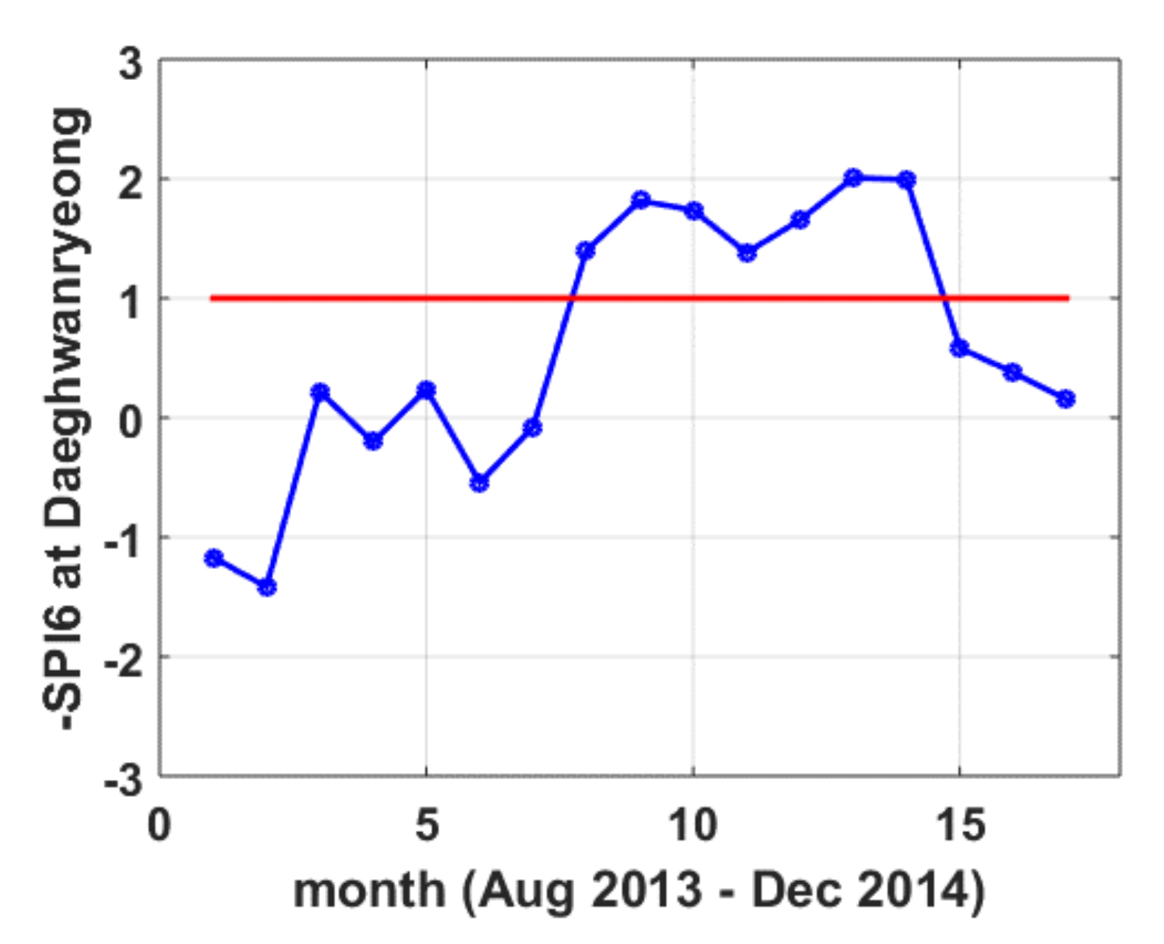
The SDF curves presented in this study can be applied to examine how the drought phenomenon is currently evolving. Figure 7 shows the SPI6 time series for the drought that lasted for 7 months from March 2014 to September 2014 on the Daeghwanryeong site.
Figure 8a shows the progress of this drought event on SDF curves created using PDS. The drought index time series for a 1 month duration from March to September 2014 is shown in the form of a solid black line and a small circle over the duration of 1 month in Figure 8a. In August 2014, it was found that the drought intensified to a maximum return level of 5.6 years. In the same way, it is possible to clearly show how the drought situation evolved over a 2-month to 7-month duration. That is, it is possible to examine how much the return level of the drought event currently in progress for each duration is. As a policy, it may be possible to standardize the largest return level at a specific point in time as the representative return level of the current drought event. When using SDF curves by PDS, it can be recognized that the drought event that occurred in 2014 started with a return level of 1.2 years for a duration of 1 month in March. It can be found that this drought event grew into a drought with a return level of 14.7 years for a duration of 4 months in June, and a severe drought with a return level of 61.2 years lasting for a duration of 7 months in September.
Monitoring of the progress of drought events can be more clearly identified using SDF curves by BED. Figure 8b is the result of expressing the same drought progress as Figure 8b using SDF curves by BED. It can be recognized that a drought event occurred in March 2014, and the drought at this time could have been characterized as a 3.6-year return period for a 1-month duration. Since then, the drought has continued to grow, deepening to a return level of 19.4 years in June, and could have been monitored for reaching a return level of 95.4 years in September.

4.3. Climate Change Drought Impact Assessment

Because global climate models (GCMs) have low spatial resolution, there are many limitations in examining future climates using GCM outputs in small areas affected by the ocean. Therefore, it is feasible to investigate the future climate using outputs from regional climate models (RCMs), which dynamically downscale the outputs of GCMs. In this study, 16 future (2021–2050) climate ensembles obtained from two GCMs (HadGEM2-AO and MPI_ESM_LR), four RCMs (RegCM4, RSM, MM5 and WRF), and two representative concentration pathway (RCP) climate change scenarios (RCP 4.5 and RCP 8.5) were applied [42].
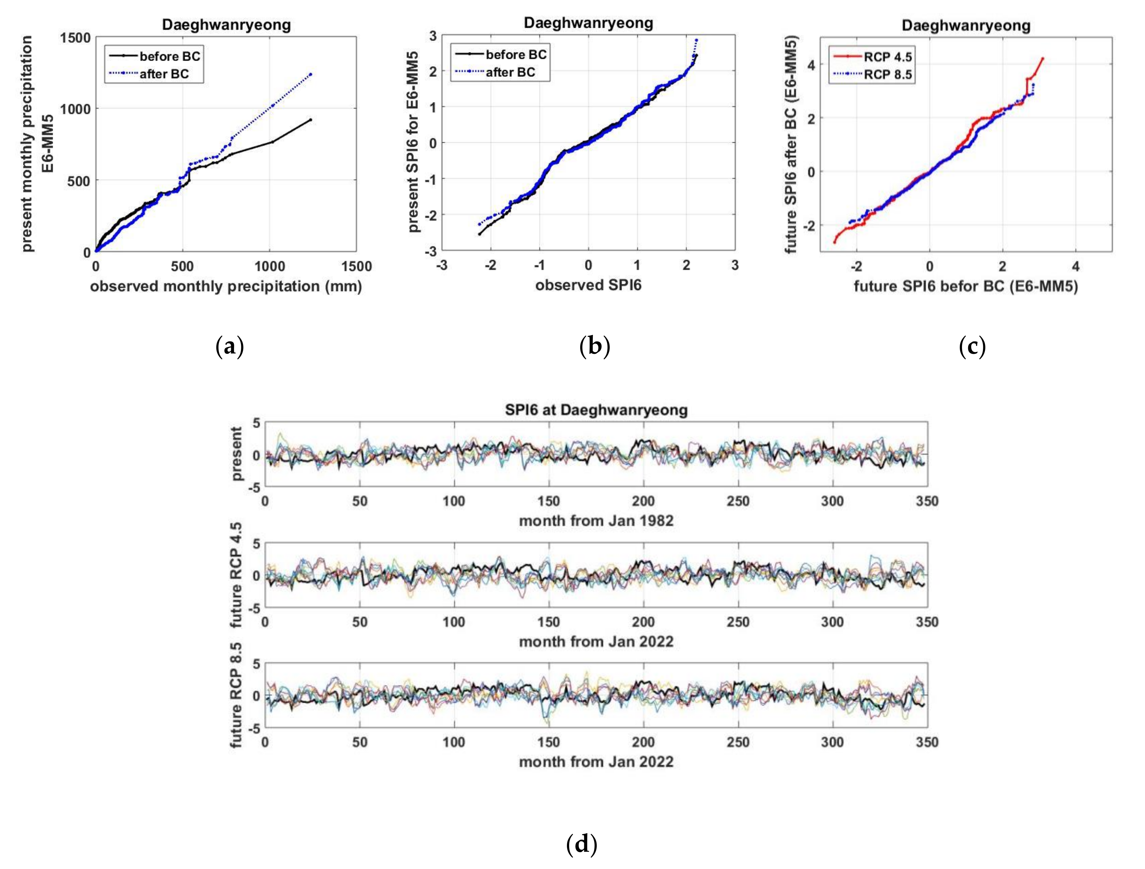
From the perspective of hydrological impact studies, RCM outputs are known to have significant biases [43,44,45]. Since bias correction is required to fit RCM outputs to observations [46], various bias-correction techniques have been developed [47]. Figure 9a shows the empirical Q–Q plot of the simulated monthly precipitation from the RCM before and after bias correction and the monthly precipitation observed in the same period. As the applied bias-correction technique, a commonly used quantile mapping technique was applied [48,49]. The climate model is a combination of MPI_ESM_LR and MM5. It can be recognized that the points of the Q–Q plot of the bias-corrected RCM monthly precipitation and the observed monthly precipitation are roughly straight. On the other hand, it can be found that the raw RCM monthly precipitation was underestimated above 500 mm. However, when calculating SPI using RCM monthly precipitation data (SPI6 in this study), it was revealed that the effect of bias correction almost disappeared (see Figure 9b,c). This is because SPI does not depend on the absolute value of monthly precipitation, but on the relative value. Therefore, in this study, the monthly precipitation simulated in RCMs without any bias correction was directly used, considering that there may be information from the RCM that is lost while performing the bias correction. Figure 9d shows the ensembles of the present and future SPI6 time series simulated at Daeghwanryeong site. The number of ensembles consists of eight for each the present condition, future condition of RCP 4.5, and future condition of RCP 8.5. For comparison, the SPI6 time series calculated using the observed monthly precipitation is shown as a thick solid line.
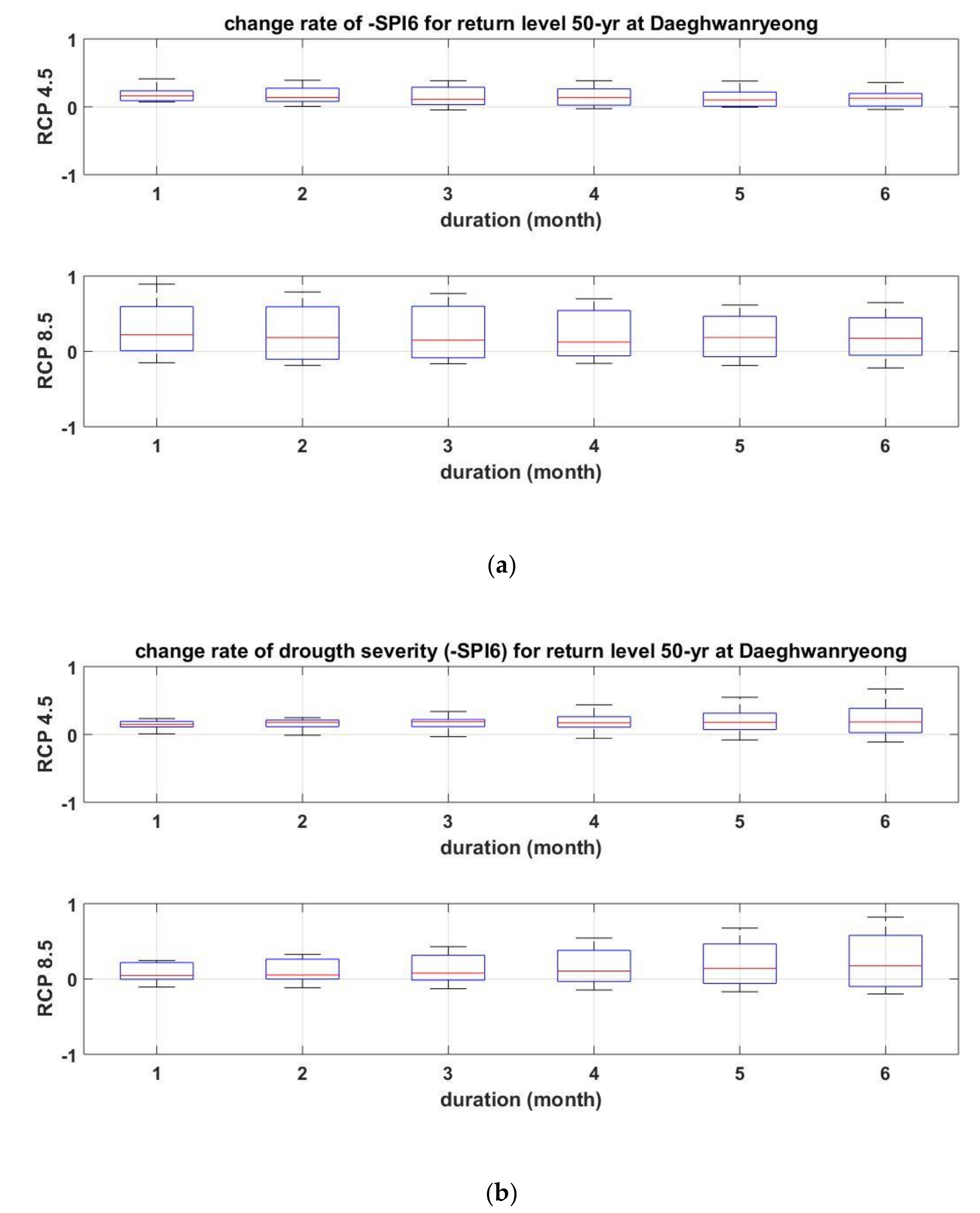
Figure 10 shows the change rate (%) of the future drought severity estimated using the projected SPI6 time series. Figure 10a shows the change rate of –SPI6 corresponding to a return level of 50 years for various durations derived from the comparison of present and future SDF curves drawn using the PDS approach. Figure 10b shows the change rate of the drought severity projected from the BED approach. In the PDS approach or the BED approach, the Daeghwanryeong site can be found to be more likely to have a drought severity 10%~20% higher than the present drought severity in the future.
Figure 10 reveals that both the PDS approach and the BED approach applied in this study can be effectively applied to investigate the prospects of future drought. In addition, when looking at the sensitivity of the change rate to the duration, in the PDS approach, the sensitivity to the duration of the change rate is not large, whereas in the BED approach, it can be found that the sensitivity of the change rate increases as the duration increases. This means that the future drought behavior of each of the PDS and BED approaches needs to be examined in more depth. In addition, the uncertainty inherent in each approach will be an important research topic. In addition, since evapotranspiration is expected to play a larger role in drought due to global warming [50], if the method proposed in this study is applied using a drought index reflecting surface air temperature, such as SPEI [51], it is expected that very interesting results will be found.

5. Conclusions

Studies looking at the return level of drought using the drought index can be broadly divided into two categories: Univariate frequency analysis using annual series extracted from drought index time series, and multivariate frequency analysis by simultaneously reflecting various characteristics of drought events. In this study, we tried to quantify the frequency of drought independently using two approaches: univariate frequency analysis and bivariate frequency analysis. In the case of univariate frequency analysis, it is important to properly consider the duration, so a partial duration series for each duration was used from the SPI time series. In the case of bivariate frequency analysis, it is necessary to satisfy both conditions that should reflect the correlation between drought severity and duration, and that should give a more realistic return level to major drought events in the past. Therefore, a relatively simple bivariate exponential distribution was used to construct a joint probability density function between drought severity and duration. SDF curves drawn from two approaches were used to examine the temporal behavior of past drought events. The SDF curves derived from the two approaches showed that they could be properly used as a tool to monitor the ongoing drought situation when a drought event occurs, although it was analyzed that both approaches require attention. The behavior of the future extreme drought considering the future climate change scenarios was investigated at the Daeghwanryeong site using two quantification methods of drought frequency analysis. Both approaches revealed that the future drought severity is likely to increase by 10% to 20% more than the present drought severity.

Supplementary Materials

The following are available online at https://www.mdpi.com/2073-4433/11/5/476/s1, Figure S1: Partial duration series, Figure S2: Empirical and Gumbel distribution function of partial duration series, Figure S3: Probability distribution of drought severity samples, Figure S4: Probability distribution of drought duration samples, Figure S5: Relation between drought severity and duration.

Author Contributions

Conceptualization, S.K.; methodology, J.W.; software, J.C.; validation, O.L. and M.J.P.; formal analysis, J.W.; investigation, J.C.; resources, O.L.; data curation, M.J.P.; writing—original draft preparation, J.W.; writing—review and editing, J.C.; visualization, O.L.; supervision, S.K.; project administration, S.K.; funding acquisition, M.J.P. All authors have read and agreed to the published version of the manuscript.

Funding

This research was funded by Korean Ministry of Interior and Safety (MOIS), grant number 2019-MOIS31-010.

Acknowledgments

This research was supported by a grant (2019-MOIS31-010) from Fundamental Technology Development Program for Extreme Disaster Response funded by Korean Ministry of Interior and Safety (MOIS).

Conflicts of Interest

The authors declare no conflict of interest.

References

  1. Chang, Y.; Kim, S.; Choi, G. A study of drought spatio-temporal characteristics using SPI-EOF analysis. J. Korea Water Resour. Assoc. 2006, 39, 691–702. [Google Scholar] [CrossRef] [Green Version]
  2. Kim, S.; Kim, B.; Ahn, T.; Kim, H. Spatio-temporal characterization of Korean drought using severity-area-duration curve analysis. Water Environ. J. 2011, 25, 22–30. [Google Scholar] [CrossRef]
  3. Yoo, C.; Kim, D. Evaluation of drought events using the rectangular pulses Poisson process model. J. Korea Water Resour. Assoc. 2006, 39, 373–382. [Google Scholar]
  4. McKee, T.; Doesken, N.; Kleist, J. Drought monitoring with multiple time scales preprints. In Proceedings of the 9th Conference on Applied Climatology, Dallas, TX, USA, 15–20 January 1995; pp. 233–236. [Google Scholar]
  5. Kim, D.; Yoo, C. Analysis of spatial distribution of droughts in Korea through drought severity-duration-frequency analysis. J. Korea Water Resour. Assoc. 2006, 39, 745–754. [Google Scholar]
  6. Ghosh, S.; Mujumdar, P. Nonparametric methods for modeling GCM and scenario uncertainty in drought assessment. Water Resour. Res. 2007, 43, W07405–W07406. [Google Scholar] [CrossRef] [Green Version]
  7. Lehner, B.; Doll, P.; Alcamo, J. Estimating the impact of global change on flood and drought risks in Europe: A continental, integrated analysis. Clim. Chang. 2008, 75, 273–299. [Google Scholar] [CrossRef]
  8. Mishra, A.; Singh, V. Analysis of drought severity-area frequency curves using a general circulation model and scenario uncertainty. J. Geophys. Res. Space Phys. 2009, 114, D06120. [Google Scholar] [CrossRef]
  9. Vidal, J.; Wade, S. A multimodel assessment of future climatological droughts in the United Kingdom. Int. J. Clim. 2007, 29, 2056–2071. [Google Scholar] [CrossRef]
  10. Lee, J.; Kim, C. Derivation of drought severity-duration-frequency curves using drought frequency analysis. J. Korea Water Resour. Assoc. 2011, 44, 889–902. [Google Scholar] [CrossRef] [Green Version]
  11. Kang, S.; Moon, J. Drought Analysis using SC-PDSI and Derivation of Drought Severity-Duration-Frequency Curves in North Korea. J. Korea Water Resour. Assoc. 2014, 47, 813–824. [Google Scholar] [CrossRef] [Green Version]
  12. Kim, C.; Park, M.; Lee, J. Analysis of climate change impacts on the spatial and frequency patterns of drought using a potential drought hazard mapping approach. Int. J. Clim. 2014, 34, 61–80. [Google Scholar] [CrossRef]
  13. Park, M.; Sim, H.; Park, Y.; Kim, S. Drought severity-duration-frequency analysis based on KMA 1-km resolution RCP Scenario. J. Korean Soc. Hazard Mitig. 2015, 15, 347–355. [Google Scholar] [CrossRef] [Green Version]
  14. Kim, J.; Lee, J.; Park, M.; Joo, J. Effect of Climate Change Scenarios and Regional Climate Models on the Drought Severity-Duration-Frequency Analysis. J. Korean Soc. Hazard Mitig. 2016, 16, 351–361. [Google Scholar] [CrossRef] [Green Version]
  15. Yoon, Y.; Park, M. Regional drought frequency analysis of monthly rainfall data by the method of L-moment. J. Korea Water Resour. Assoc. 1997, 30, 55–62. [Google Scholar]
  16. Kao, S.; Govindaraju, R. A copula-based joint deficit index for droughts. J. Hydrol. 2010, 380, 121–134. [Google Scholar] [CrossRef]
  17. Dalezios, N.; Loukas, A.; Vasiliades, L.; Liakopoulos, E. Severity-duration-frequency analysis of droughts and wet periods in Greece. Hydrol. Sci. J. 2000, 45, 751–769. [Google Scholar] [CrossRef]
  18. Palmer, W. Meteorological Drought; U.S. Department of Commerce: Washington, DC, USA, 1965.
  19. Shiau, J.; Shen, H. Recurrence analysis of hydrologic droughts of differing severity. J. Water Resour. Plan. Manag. 2001, 127, 30–40. [Google Scholar] [CrossRef]
  20. Shiau, J. Fitting drought duration and severity with two-dimensional copulas. Water Resour. Manag. 2006, 20, 795–815. [Google Scholar] [CrossRef]
  21. Yeon, J.; Byun, S.; Lee, J.; Kim, T. Evaluation of droughts in Seoul using two-dimensional drought frequency analysis. J. Korea Water Resour. Assoc. 2007, 40, 335–343. [Google Scholar] [CrossRef]
  22. Shiau, J.; Modarres, R. Copula-based drought severity–duration-frequency analysis in Iran. Meteorol. Appl. 2009, 16, 481–489. [Google Scholar] [CrossRef]
  23. Ganguli, P.; Reddy, M. Risk assessment of droughts in Gujarat using bivariate copulas. Water Resour. Manag. 2012, 26, 3301–3327. [Google Scholar] [CrossRef]
  24. Mirabbasi, R.; Fakheri-Fard, A.; Dinpashoh, Y. Bivariate drought frequency analysis using the copula method. Theor. Appl. Clim. 2012, 108, 191–206. [Google Scholar] [CrossRef]
  25. Chen, L.; Singh, V.; Guo, S.; Mishra, A.; Guo, J. Drought analysis using copulas. J. Hydrol. Eng. 2013, 18, 797–808. [Google Scholar] [CrossRef]
  26. Halwatura, D.; Lechner, A.; Arnold, S. Drought severity–duration-frequency curves: A foundation for risk assessment and planning tool for ecosystem establishment in post-mining landscape. Hydrol. Earth Syst. Sci. 2015, 19, 1069–1091. [Google Scholar] [CrossRef] [Green Version]
  27. Chun, S.; Kim, Y.; Kwon, H. Drought frequency analysis using hidden markov chain model and bivariate copula function. J. Korea Water Resour. Assoc. 2015, 48, 969–979. [Google Scholar] [CrossRef]
  28. Kim, J.; So, B.; Kim, T.; Kwon, H. A development of trivariate drought frequency analysis approach using copula function. J. Korea Water Resour. Assoc. 2016, 49, 823–833. [Google Scholar]
  29. Yu, J.; Yoo, J.; Lee, J.; Kim, T. Estimation of drought risk through the bivariate drought frequency analysis using copula functions. J. Korea Water Resour. Assoc. 2016, 49, 217–225. [Google Scholar] [CrossRef]
  30. Kwon, M.; Sung, J.; Kim, T.; Ahn, J. Drought assessment by bivariate frequency analysis using standardized precipitation index and precipitation deficit: Focused on Han river basin. J. Korea Water Resour. Assoc. 2018, 51, 875–886. [Google Scholar]
  31. Ryu, J.; Ahn, J.; Kim, S. An application of drought severity-area-duration curves using copulas-based joint drought index. J. Korea Water Resour. Assoc. 2012, 45, 1043–1050. [Google Scholar] [CrossRef]
  32. Stall, J. Low Flows of Illinois Streams for Impounding Reservoir Design, Bulletin 51; Illinois State Water Survey: Champaign, IL, USA, 1964. [Google Scholar]
  33. WMO. Experts Agree on a Universal Drought Index to Cope with Climate Risks. World Meteorological Organization Press Release No. 872. Available online: http://www.mondialisations.org/php/public/art.php?id=32782lan=EN&lan=EN (accessed on 28 July 2019).
  34. KMA. Hydro-Meteorologic Drought Information System. Available online: https://hydro.kma.go.kr/help/menu200.do (accessed on 3 August 2019).
  35. Hosking, J. L-moments: Analysis and estimation of distributions using linear combinations of order statistics. J. R. Stat. Soc. 1990, 52, 105–124. [Google Scholar] [CrossRef]
  36. Yevjevich, V. Objective Approach to Definitions and Investigations of Continental Hydrologic Droughts; Hydrology Paper 23; Colorado State University: Fort Collins, CO, USA, 1967. [Google Scholar]
  37. Nagao, M.; Kadoya, M. Two variate exponential distribution and its numerical table for engineering applications. Bull. Disaster Prev. Res. Inst. 1971, 20, 183–215. [Google Scholar]
  38. Yue, S. Applicability of the Nagao–Kadoya bivariate exponential distribution for modeling two correlated exponentially distributed variates. Stoch. Environ. Res. Risk Assess. 2001, 15, 244–260. [Google Scholar] [CrossRef]
  39. Cordova, J.; Rodriguez-Iturbe, I. On the probabilistic structure of storm surface runoff. Water Resour. Res. 1985, 21, 755–763. [Google Scholar] [CrossRef]
  40. Goel, N.; Kurothe, R.; Mathur, B.; Vogel, R. A derived flood frequency distribution for correlated rainfall intensity and duration. J. Hydrol. 2000, 228, 56–67. [Google Scholar] [CrossRef]
  41. Ashkar, F.; Jabi, N.; Issa, M. A bivariate analysis of the volume and duration of low-flow events. Stoch. Environ. Res. Risk Assess. 1998, 12, 97–116. [Google Scholar] [CrossRef]
  42. Park, C.; Cha, D.; Kim, G.; Lee, G.; Lee, D.; Suh, M.; Hong, S.; Ahn, J.; Min, S. Evaluation of summer precipitation over Far East Asia and South Korea simulated by multiple regional climate models. Int. J. Clim. 2019. [Google Scholar] [CrossRef]
  43. Teutschbein, C.; Seibert, J. Regional climate models for hydrological impact studies at the catchment scale: A review of recent modeling strategies. Geogr. Compass 2010, 4, 834–860. [Google Scholar] [CrossRef] [Green Version]
  44. Arnbjerg-Nielsen, K.; Willems, P.; Olsson, J.; Beecham, S.; Pathirana, A.; Gregersen, I.; Madsen, H.; Nguyen, V. Impacts of climate change on rainfall extremes and urban drainage systems: A review. Water Sci. Technol. 2013, 68, 16–28. [Google Scholar] [CrossRef]
  45. Lee, O.; Sim, I.; Kim, S. Application of the non-stationary peak-over-threshold methods for deriving rainfall extremes from temperature projections. J. Hydrol. 2019. [Google Scholar] [CrossRef]
  46. Li, J.; Evans, J.; Johnson, F.; Sharma, A. A comparison of methods for estimating climate change impact on design rainfall using a high-resolution RCM. J. Hydrol. 2017, 547, 413–427. [Google Scholar] [CrossRef]
  47. Lenderink, G.; Fowler, H. Hydroclimate: Understanding rainfall extremes. Nat. Clim. Chang. 2017, 7, 391–393. [Google Scholar] [CrossRef] [Green Version]
  48. Lee, O.; Kim, S. Estimation of Future Probable Maximum Precipitation in Korea Using Multiple Regional Climate Models. Water 2018, 10, 637. [Google Scholar] [CrossRef] [Green Version]
  49. Choi, J.; Lee, O.; Jang, J.; Jang, S.; Kim, S. Future intensity–depth–frequency curves estimation in Korea under representative concentration pathway scenarios of Fifth assessment report using scale-invariance method. Int. J. Clim. 2019, 39, 887–900. [Google Scholar] [CrossRef]
  50. Spinoni, J.; Barbosa, P.; Bucchignani, E.; Cassano, J.; Cavazos, T.; Christensen, J.; Christensen, O.; Coppola, E.; Evans, J.; Geyer, B.; et al. Future global meteorological drought hot spots: A study based on CORDEX Data. J. Clim. 2020, 33, 3635–3661. [Google Scholar] [CrossRef]
  51. Vicente-Serrano, S.; Beguería, S.; López-Moreno, J. A multiscalar drought index sensitive to global warming: The standardized precipitation evapotranspiration index. J. Clim. 2010, 23, 1696–1718. [Google Scholar] [CrossRef] [Green Version]
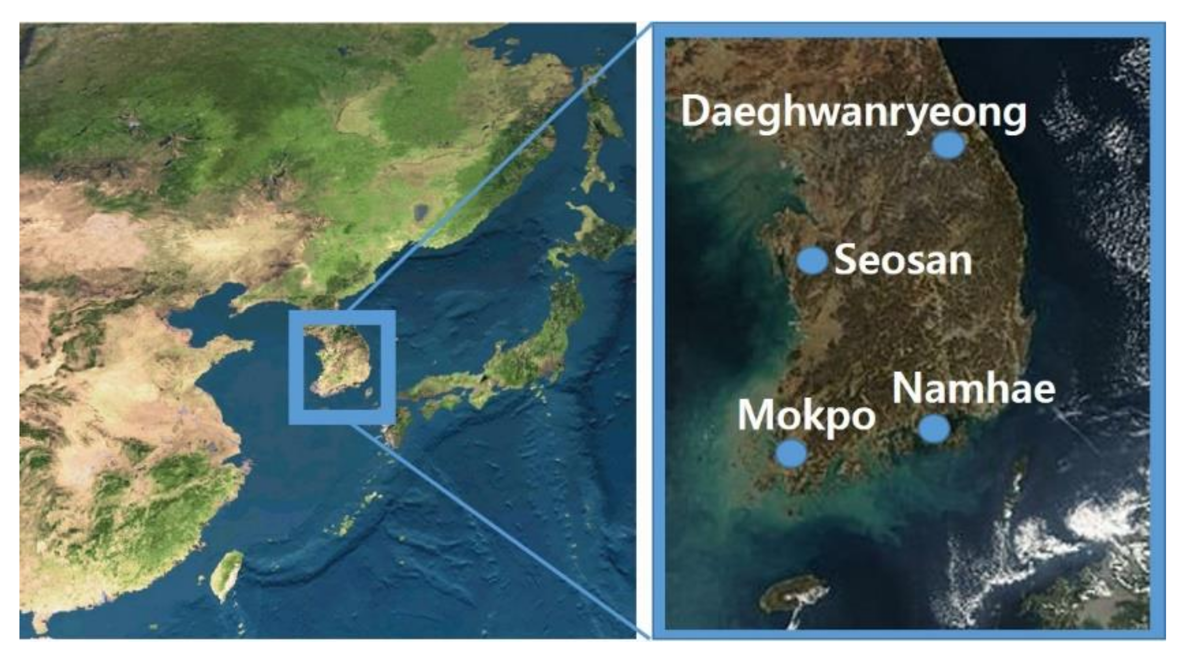
Figure 1. Location of study precipitation sites.
Atmosphere 11 00476 g001
Figure 2. SPI monthly time series at (a) Daeghwanryeong, (b) Mokpo, (c) Namhae, and (d) Seosan. For reference, the red line indicates SPI’s drought criterion of −1.
Atmosphere 11 00476 g002
Figure 3. Concept of drought event.
Atmosphere 11 00476 g003
Figure 4. SDF curves using partial duration series at (a) Daeghwanryeong, (b) Mokpo, (c) Namhae, and (d) Seosan. In Figure 4, + is the drought index observed to be the most severe during the 37-year period for a specific duration, and x is the drought index observed to be the seventh most severe.
Atmosphere 11 00476 g004
Figure 5. Joint probability density function of drought severity and duration at (a) Daeghwanryeong, (b) Mokpo, (c) Namhae, and (d) Seosan.
Atmosphere 11 00476 g005
Figure 6. SDF curves using bivariate exponential distribution at (a) Daeghwanryeong, (b) Mokpo, (c) Namhae, and (d) Seosan. In Figure 6, * indicates the drought severity and duration of the observed drought events.
Atmosphere 11 00476 g006
Figure 7. SPI6 time series for a drought event at Daeghwanryeong site.
Atmosphere 11 00476 g007
Figure 8. Drought situation monitoring using SDF curves based on (a) partial duration series and (b) bivariate exponential distribution.
Atmosphere 11 00476 g008
Figure 9. Future SPI6 projection: (a) Monthly precipitation; (b) Present SPI; (c) Future SPI; (d) Present and future SPI6 time series ensemble.
Atmosphere 11 00476 g009
Figure 10. Change rate of drought severity for a return level of 50 years at the Daeghwanryeong site using (a) PDS approach, and (b) BED approach.
Atmosphere 11 00476 g010
Table 1. Number of partial duration series.
SiteDaeghwanryeongMokpoNamhaeSeosan
Duration
1 month37373737
2 months37373737
3 months37373737
4 months37373737
5 months37373737
6 months36343736
7 months31293134
8 months25282631
9 months24242329
10 months23202024
11 months22172020
12 months21161717
Table 2. Date when the most extreme drought index occurred.
SiteDaeghwanryeongMokpoNamhaeSeosan
Duration
1 monthMay 2001Apr. 2000Mar. 1984May 2001
2 monthsMay 2001May 2000Mar. 1984Jun. 2017
3 monthsOct. 2015May 2000Mar. 1984Jun. 2017
4 monthsOct. 2015Dec. 1988Apr. 1984Jun. 2017
5 monthsOct. 2015Dec. 1988May 1984Jul. 2017
6 monthsSep. 2014Sep. 1994May 1984Aug. 2017
7 monthsSep. 2014Sep. 1994Jun. 1984Sep. 2017
8 monthsOct. 2014Sep. 1994Jul. 1984Nov. 2017
9 monthsNov. 2014Oct. 1994Aug. 1984Nov. 2017
10 monthsDec. 2014Feb. 1996Sep. 1984Nov. 1988
11 monthsJan. 2015Feb. 1996Oct. 1984Dec. 1988
12 monthsFeb. 2015Feb. 1996Nov. 1984Dec. 1988
Table 3. Statistics of drought events.
SiteNumber of EventsSeverity (-)Duration (Month)
MeanStandard
Deviation
MeanStandard
Deviation
Daeghwanryeong380.44620.38981.76321.2398
Mokpo330.40980.34891.96971.8789
Namhae330.45000.35022.03031.4892
Seosan350.46360.35411.62861.0596
Table 4. Most extreme drought events.
SiteDaeghwan-RyeongMokpoNamhaeSeosan
Maximum
severity
event
Mean value
of –SPI
2.57942.28992.37262.3233
Duration
(month)
2112
Occurrence
date
2001/042001/051989/052001/04
Return level
(year)
33.626.123.718.4
Maximum
Duration
event
Duration
(month)
7765
Mean value
of –SPI
1.71271.73471.92221.3078
Occurrence
date
2014/031994/031983/122007/12
Return level
(year)
51.639.221.522.8