1. Introduction
Currently, more people are affected by flash floods than any other type of natural disaster [
1,
2,
3]. In recent years, the most populated cities have been affected by floods and flash floods that directly or indirectly impact the socioeconomic development of the population. For example, São Paulo, known as the most populated city in Brazil, has frequent flash floods caused by several factors that are sometimes related to the hydrographic basin, local catchments, and local effects like the topography and soil coverage. In the summer of 2014/2015, the traffic vehicle department of São Paulo observed 183 flooding points, and 130 flooding events occurred between January and March 2015.
To reduce hydro-geological risk from flash floods, several studies have implemented methodologies that monitor and analyze the behavior of rainfall to implement a flash flood warning system. Flash flood forecasting algorithms are commonly based on hydrological or hydraulic models [
4,
5,
6,
7], numerical simulation models [
3,
8,
9,
10], and Machine Learning algorithms such as the Artificial Neural Network [
11,
12,
13,
14], Support Vector Machines [
15], Adaptive Neuro-Fuzzy Inference Systems (ANFIS) [
16], or Random Forest [
2,
17]. Likewise, Mosavi et al. [
18] demonstrated the advantages of certain Machine Learning algorithms through a qualitative analysis. In this study, they considered the flood resource variable, such as water levels, precipitation or streamflow, and the prediction type. Based on the correlation coefficient (R
2) and root mean square error (RMSE) evaluation, they concluded that combining two or more methods, by using data decomposition techniques or using add-on optimizer algorithms, improve the flood prediction for short-term and long-term predictions.
However, there are hardly any studies on flash flood forecasting using regression applications as they are usually focused on a numerical forecasting of flash flood events [
19]. The logistic regression with a binary response is simply a designation of one of two possible outcomes. It means that we have a prediction of a chance or a probability. Studies in landslides [
20,
21] or hail risk [
22,
23] demonstrate the efficiency of logistic regression for predicting the probability of occurrence.
In São Paulo city, the Flood Alert System of São Paulo (SAISP), operated by the Technological Center of the Hydraulics Foundation (FCTH), monitors flood events by integrating a dual-band S Doppler radar polarization and telemetry. For flood forecasting, SAISP uses a hydrological model called SWMM (Storm Water Management Model) that generates flood maps and shows affected areas in the São Paulo Metropolitan Region (RMSP) [
24]. The model was validated by Sosnoski et al. [
25], and the results showed that it can be a useful tool for delimiting flood areas. This information is reported to various agencies, especially to the Climate Emergency Management Center (CGE), which also gathers information from weather stations, rain gauges, and local observations in order to monitor the points of the flood.
According to the study of Viteri [
26], who used radar measurements with flash flood events and points, flash flood events in São Paulo are associated with a rainfall volume greater than 30 mm per day and a maximum rainfall rate greater than 30 mmh
−1. Furthermore, neighborhoods located near the Tietê and Pinheiros rivers and in the central region of São Paulo city presented higher probability of the occurrence of flash floods when there were rainfall volumes lower than the average of 30 mm per day in addition to presenting a higher recurrence of flood points.
Based on these features, this study aims to estimate the probability of occurrence of flash floods in São Paulo city considering its watersheds. In order to do this, the study presents a binary logistic regression model that combines rain estimates from the dual-polarization S-band Doppler meteorological weather radar (SPOL) from the Departamento de Águas e Energia Elétrica (DAEE) and the FCTH and flooding points observed by the CGE during the occurrence/non-occurrence of flash flood events.
2. Data and Methodology
2.1. Study Area
The study area is the city of São Paulo located in the state of São Paulo in Southeast Brazil. São Paulo is the biggest city of São Paulo Metropolitan Region (SPMR) with an area of 1521 km
2 and approximately 12.1 million people. SPMR includes 39 municipalities and represents the largest industrial complex and urban concentration in Latin America [
24].
The city of São Paulo is divided into 96 districts with a mean altitude of 760 m along the Tietê River basin, which is divided into Upper, Middle, and Lower Tietê and is the major water source of SPMR. The Upper Tietê river basin, where the city of São Paulo is located, has a drainage area of 5720 km2. There are seven dams in which two control the Tietê river flow, and the other five contribute to the Upper Tietê Producer System in SPMR. The Ponte Nova Dam, which is located in Southeast SPMR, has the major drained area of 320 km2 with a discharge of 3.9 m3/s, which is followed by Taiaçupeba with 224 km2 drained area and 0.5 m3/s discharge.
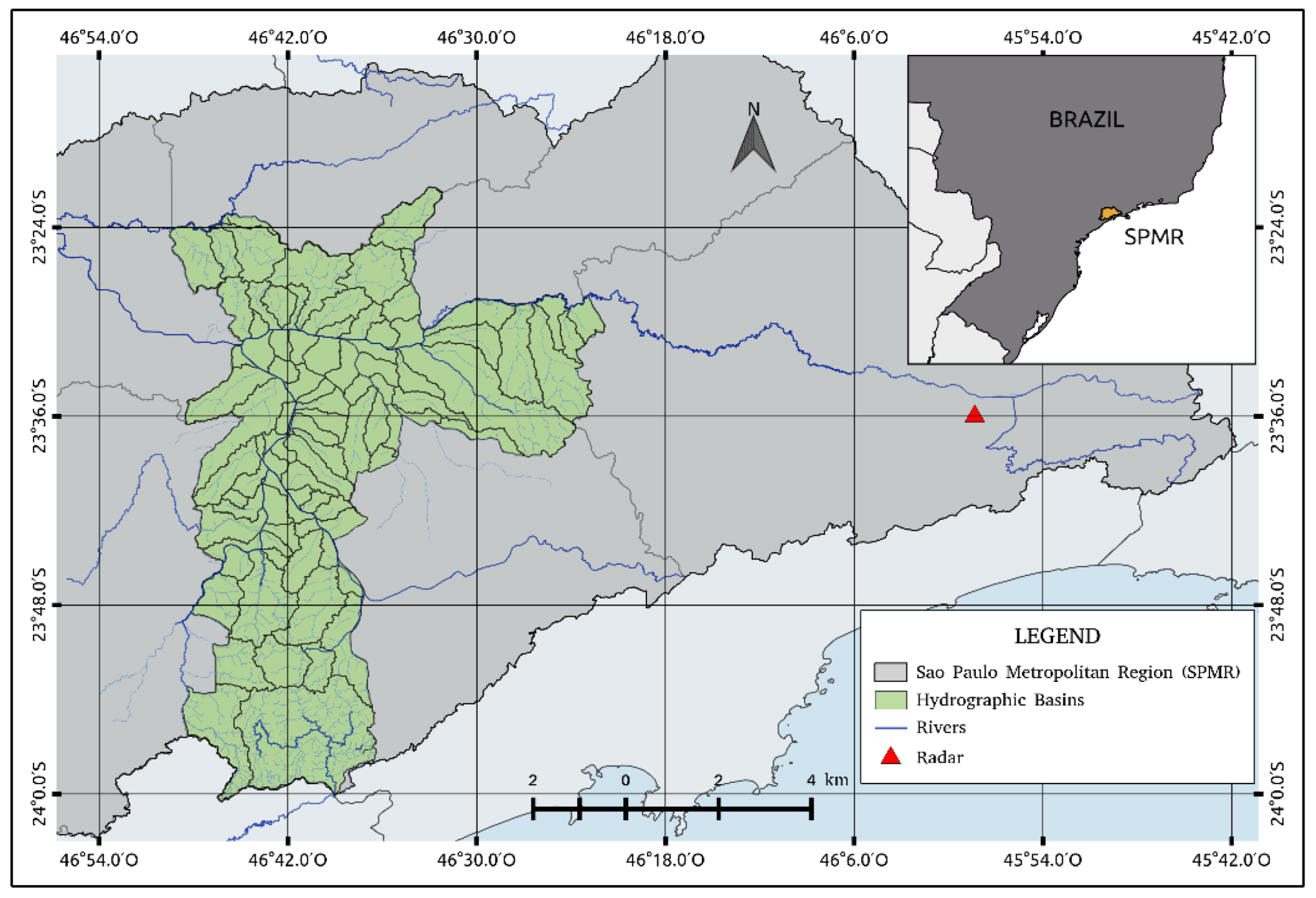
In total, São Paulo has more than 300 rivers (surface and canalized) that form the relief of each watershed. The Pinheiros and Tamanduateí rivers are the main tributaries of the Tietê river in the topography of 186 watersheds in the city, as seen in
Figure 1. For example, the Aricanduva river is located in the eastern region of São Paulo and has an approximate drained area of 100.4 km
2. The Pirajucara river, which is located in the western zone, has a drained area of 72 km
2. The Mandaqui river is a basin located in the northern region of the city that is almost completely urbanized, and has a drained area of 18.6 km
2 [
5].
Cold fronts, squall lines, sea breezes, and local convection are the main meteorological systems contributing to precipitation in the city of São Paulo and surrounding areas [
26]. Annually, São Paulo has a precipitation of more than 1200 mm, and, during summer time (December-March), it varies from 450 mm to 700 mm. Due to the large number of impermeable areas, which increase the surface runoff, flash floods are frequent every year [
27], especially in the rainy season, from October to March.
2.2. Rainfall Measurements
This study uses rain estimates obtained from a dual-polarization S-band Doppler weather radar (SPOL), model METEOR 600S from Selex, operated by the DAEE and the FCTH at the Ponte Nova dam, 70 km from São Paulo (
Figure 1) for the 2015–2016 period. This radar is configured to scan a 240-km radius every 5 min with eight elevations, and with a gate resolution of 250 m.
For this study, we used the Dual Polarization Surface Rainfall Intensity (DPSRI) algorithm [
28] to retrieve the rain estimates with a resolution of 500 × 500 m. In summary, the DPSRI algorithm uses radar reflectivity (Z), differential reflectivity (ZDR), and the specific differential phase (KDP) variables to estimate the rainfall rate in a Pseudo-DPSRI mode [
29].
According to Viteri [
30], the rainfall estimates used in this study were compared to a rain gauge network and presented a bias score (BIAS) of 31% for 10 min, 50% for one hour, and 89% for one day integration time. The RMSE varies from 16.3 mm for 10 min, 0.5 mm for one hour, and 6.6 mm for one day. The correlation coefficient provides a better fit for a timescale of one day, i.e., 0.8, which is followed by one hour with 0.7 and finally for 10 min with 0.4. Therefore, 24 h accumulated precipitation represents the best SPOL weather radar rain estimates.
2.3. Flash Flood Measurements
According to the National Center for Risk and Disaster Management (CENAD) [
31], floods are hydrological phenomena caused by an excess capacity of surface runoff and urban drainage systems forming accumulations of water in impermeable areas. Faced with the chaotic urban expansion process, recurrent floods are observed in areas that lack favorable conditions for infiltration and runoff. For instance, during the summertime, São Paulo is frequently affected by flash floods that have tremendous economic impacts and increase the vulnerability of various neighborhoods with poor infrastructures. For example,
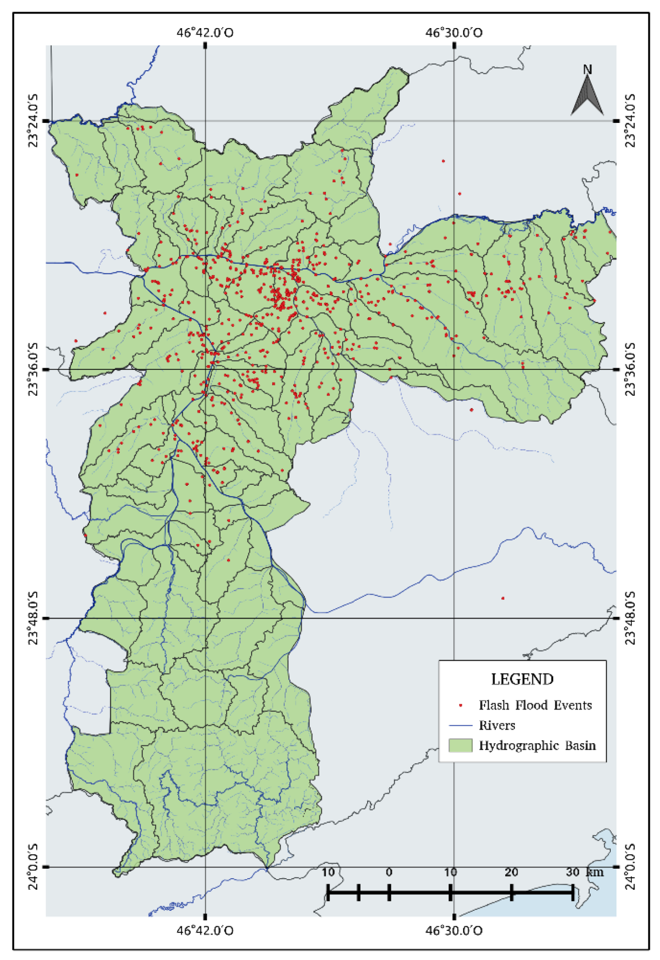
Figure 2 shows the location of recorded flash floods in the period of 2015 and 2016. Most of the flash floods are observed along the Pinheiros and Tietê rivers as well as in other regions except for the southern region that does not show any events due to the absence of observations [
26]. In 2015, there were 224 days with rain and 100 flood events, while, in 2016, there were 214 rainy days and 110 inundations.
To overcome this recurrent problem, São Paulo City Hall deployed the Climate Emergency Management Center (CGE) to monitor flood areas in the city of São Paulo and mitigate the effects. Basically, the CGE uses the SPOL radar and rain gauge measurements available from the FCTH and flood indications provided by the Municipal Civil Defense Coordination (COMDEC) and the Traffic Engineering Company (CET). For this study, we have used a flood inventory database from 2015 to 2016 provided by the CGE to adjust a binary logistic regression model to predict floods. The database contains the location, time of the occurrence, and a description of the events whenever available.
2.4. Binary Logistic Regression Model
The probability of the occurrence of flash floods was obtained by the logistic regression model [
32] (
Figure 3) described on Equations (1–3). The logistic regression analyzes the association between two qualitative variables, which include one dependent variable and one independent variable (exploratory), without assuming a linear relationship. The dependent variable has only two values, such as presence or absence, success or failure, or an event occurring or not occurring. The independent variable can be continuous, discrete, or both [
21,
33]. The predictable output variable calculated has values of 0 or 1. For this study, zero means 0% probability of flash flood occurrence and one means 100% probability of flash flood occurrence.
The logistic regression model is based on the logistic function f(z), which is defined as:
where z is the net input, that is, the linear combination of weights (β) and sample features (x) and can be calculated by the equation below.
In terms of probability, this function can be written by the logit transformation, which has a relatively simple mathematical form.
where the odds ratio or likelihood ratio and p(x) are the probabilities of the event occurrence. Instead of using the least squared deviations for the best fit, the coefficients β are estimated by using the maximum likelihood method, which maximizes the probability of occurrence of flash floods given the fitted regression coefficients.
2.5. Methodology
Figure 4 shows a flowchart of how the model is configured. First, the rainfall field measurements are obtained from the SPOL DPSRI algorithm. Second, the model uses daily accumulated precipitation, the maximum precipitation rate [mm/h], and total rainfall duration [min] registered in the previous 24 h.
To increase the number of samples and also to be equally distributed, the rainfall and flood database was divided into two sets: 2015 was used to adjust the model while 2016 was used for validation. Both datasets have flash flood and non-flash flood events. Finally, it is important to observe that the model output values vary from 0 to 1. Days with no occurrence of flash floods have been assigned to have a probability lower than 0.5, and those with a flash flood above 0.5.
Moreover, in order to improve the accuracy of the probability, we applied the Akaike Information Criterion (AIC) [
34] to select the best predictor variables for each watershed. Good model performance is that which has the minimum AIC value of all other model combinations. In our case, we can have seven combinations (
Table 1) including three, two, and one predictor variables (A: Accumulated precipitation, B: maximum precipitation rate, and C: rainfall duration). For the example shown in
Table 1, the maximum AIC had three and two variables A–C, while variable B presents the lowest AIC value. Therefore, variable B (maximum precipitation) represents the best variable to predict flash floods.
Lastly, in order to validate the logistic model, we employed the contingency table [
35] method to compute the bias score (BIAS), the probability of detection (POD), the false alarm ratio (FAR), and the critical success index (CSI).
The BIAS is an indicator of how well the estimate predicts the number of occurrences of an event. The POD is defined as the percentage of correct answers when estimating the occurrence of the event, and it varies from 0 to 1, where 1 means the optimal performance. The POD is commonly known as the hit rate. The FAR is defined as the percentage in which the event did not occur and varied between 0 and 1. Furthermore, 0 means the best performance. The CSI index is defined as the percentage of correct answers in the estimates, and it varies between 0 and 1, with higher values representing better performance. In addition, the POD and FAR were combined to compute the Relative Operating Characteristic (ROC) [
36] in order to verify the probabilistic forecast and to understand issues related to accuracy, criterion selection, and interpretation [
21].
3. Results
In 2015 and 2016, more than 2000 flash flood points were registered by the CGE. Flash flood warnings were more frequent in the summertime, and were concentrated in the western, southern, and central regions of the city of São Paulo with a great number of recurrent locations (
Figure 2).
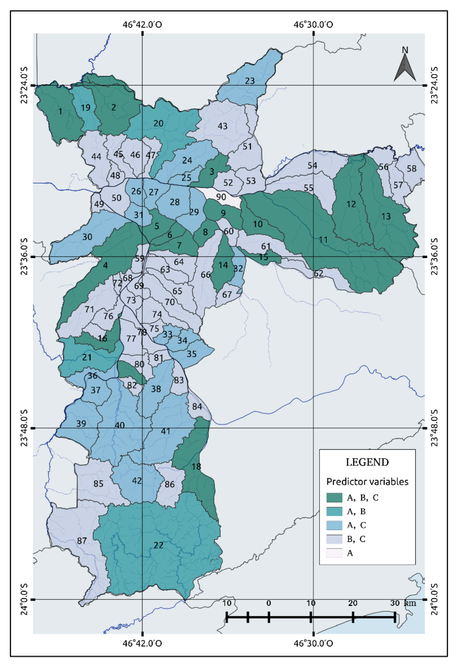
In this study, we have considered only 90 watersheds that registered more than two flood points in order to estimate the probability of the occurrence of flash floods.
Figure 5 summarizes the watershed selected with an indication of the number of predictor variables and respective index to consult the model coefficients (
Appendix A,
Table A1,
Table A2,
Table A3,
Table A4 and
Table A5). As explained in the previous section, AIC criteria were used to determine the best predictor variables to predict flash floods.
After the model validation, we obtained the predictor variables for each watershed and computed the probability by using Equation (4). For instance, the model uses the following parameters (
): (
) accumulated precipitation, (
) maximum precipitation rate, and (
) rainfall duration together with the coefficients (
) calculated from the logistic regression model presented in
Appendix A.
Moreover,
Table A1,
Table A2,
Table A3,
Table A4 and
Table A5 in
Appendix A also shows the accuracy of each watershed model. The accuracy ranged from 80 to 98% with a mean value of 86%. The p-values associated with the correlation of variables in each model are very small in some cases, which indicates their good association with the probability of flash floods. A significant p-value was found in 96% of the watersheds with a value of less than 0.8. Taking into account the rain estimates errors found by Viteri [
26], the uncertainty of the model in predicting the probability will be less than 10
–5 and, therefore, would not affect the flash flood prediction.
Analyzing
Figure 5, it is possible to observe that most of the watersheds can be adjusted by two variables, i.e., maximum precipitation rate and rainfall duration (B,C), which is followed by 20 watersheds that use daily precipitation and rainfall duration (A,C), and four watersheds with accumulated precipitation and a maximum precipitation rate (A,B). Eighteen watersheds need the three variables, while only one watershed depends on only one variable, i.e., accumulated precipitation. Watersheds related to the predictor A tend to have flash flood occurrence with an average of 20 mm per day. Predictor B did not show any significant pattern. The highest values registered were located in the south, and two or three watersheds in the north and central regions (watersheds index 9, 18, 20, 21, 22, 42, and 60) with an average of 190 mm/h. Predictor C, on the other hand, is related to shorter rainfall durations since the maximum values were located in the watersheds not associated with this predictor variable.
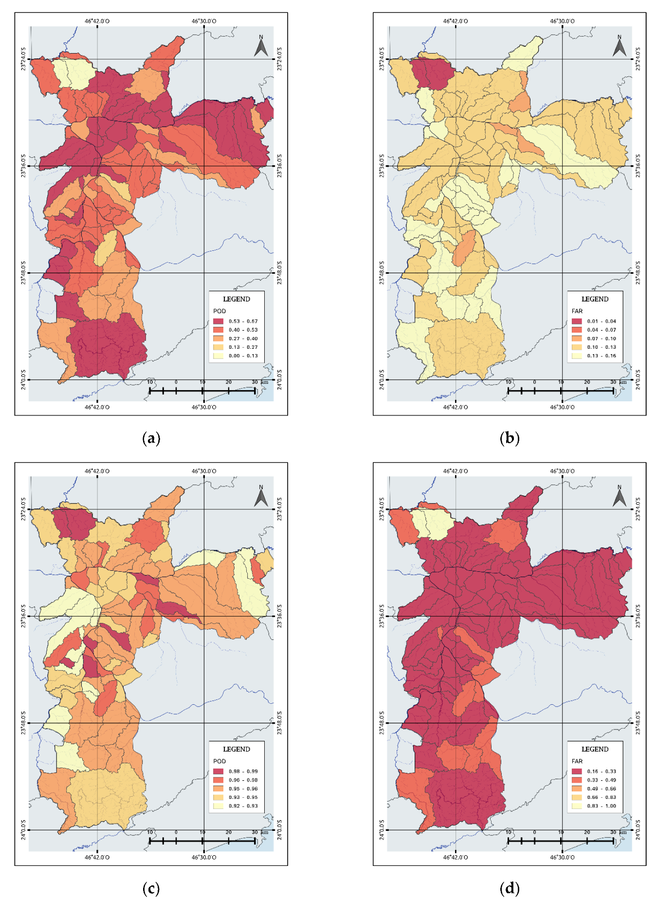
Figure 6 presents how the POD and FAR vary as functions of flash flood occurrence in each watershed. For flash flood events, the mean POD was 0.46, and the FAR was 0.12. The POD (
Figure 6a) and FAR (
Figure 6b) spatial distribution maps show several regions with acceptable performance (POD > 0.5). Watersheds with a lower POD are observed in the northern part of the city with a POD, but with a higher probability of non-flash flood occurrence (
Figure 6c). These watersheds correspond to the Jaraguá and Perus neighborhoods, which registered 7 (1) and 1 (4) days with flash flood events, respectively, in 2015 (2016) at a maximum precipitation rate of 59 mm/h. Almost 48% of the watersheds located in the eastern part of the city and near the Tietê and Pinheiros Rivers, presented more than 50% POD that could be related to their recurrent flash flood events and the different infiltration capacity [
30], which means ground capacity to absorb rain water.
The FAR map increases from 0.01 to 0.16 and demonstrates that few watersheds have predicted flash flood events that were not observed. For example, two watersheds located in the north obtained a good FAR value while 30% of the watersheds showed the FAR varying from 0.13 to 0.16. Most of them are concentrated in the south.
On the other hand, the POD and FAR for no occurrence of flash floods events (
Figure 6c,d), respectively, show better results. The POD increases from 0.92 to 1 while the mean FAR is 0.297 (
Table 2). According to
Figure 6c, near the Tietê River, the probability of non-flash flood occurrence is higher, particularly in the neighborhoods of Pari and Belém, with a probability of 99%. At the edge of the River Pinheiros, we can observe watersheds with the high probability of non-occurrence, like Santo Amaro and Itaim Bibi, which registered 25 and 5 days with flash flood events. On the other hand, low POD values were observed in the eastern and southwestern districts and ranged from 0.92 to 0.93.
Moreover,
Table 2 presents the average scores for events with and without flash flood occurrence using conditional (only rainy days) and unconditional rainy days (all days). From these scores, it is possible to note that the proposed model has a better performance to predict no flash flood events (BIAS, POD, and CSI), but, when only rain days are used, the model improved the prediction of flash flood events to 71%.
Comparing the average scores calculated for both situations, the logistic model has a better performance to predict the non-occurrence of flash floods (POD and CSI) even though it is possible to predict flash flood events with a 71% success rate when considering only rainy days.
Case Study: 11 March 2016
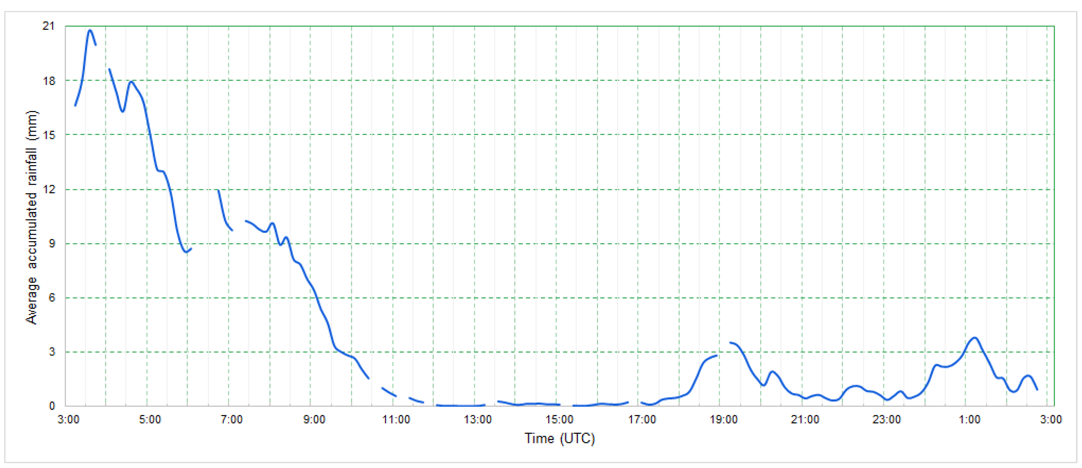
On March 11, 2016, a storm produced the largest flood peak in the city of São Paulo during the observation period. As noted in
Figure 7, the maximum hourly accumulated rainfall occurred between 00:00 HL and 01:00 HL. The maximum 10 min accumulated rainfall was 20.7 mm, and the city registered 175 mmh
−1 of a maximum precipitation rate. Like many urban flash floods in the city, this event was associated with a passage of a surface cold front associated with the South Atlantic Convergence Zone (SACZ), which usually show large rain volumes for long periods of time [
37,
38].
This event produced flash flooding in the city, mainly in the Tietê and Pinheiros rivers overflow, which resulted in several landslides and damaged the city’s infrastructure. The traffic vehicle department of São Paulo observed 93 flooding points around the city. The northern and western zones recorded the highest flash flood rate with 32 flood points, which was followed by the southern, central, eastern, and southeastern zones with 10, 9, 7, and 3 flood points, respectively.
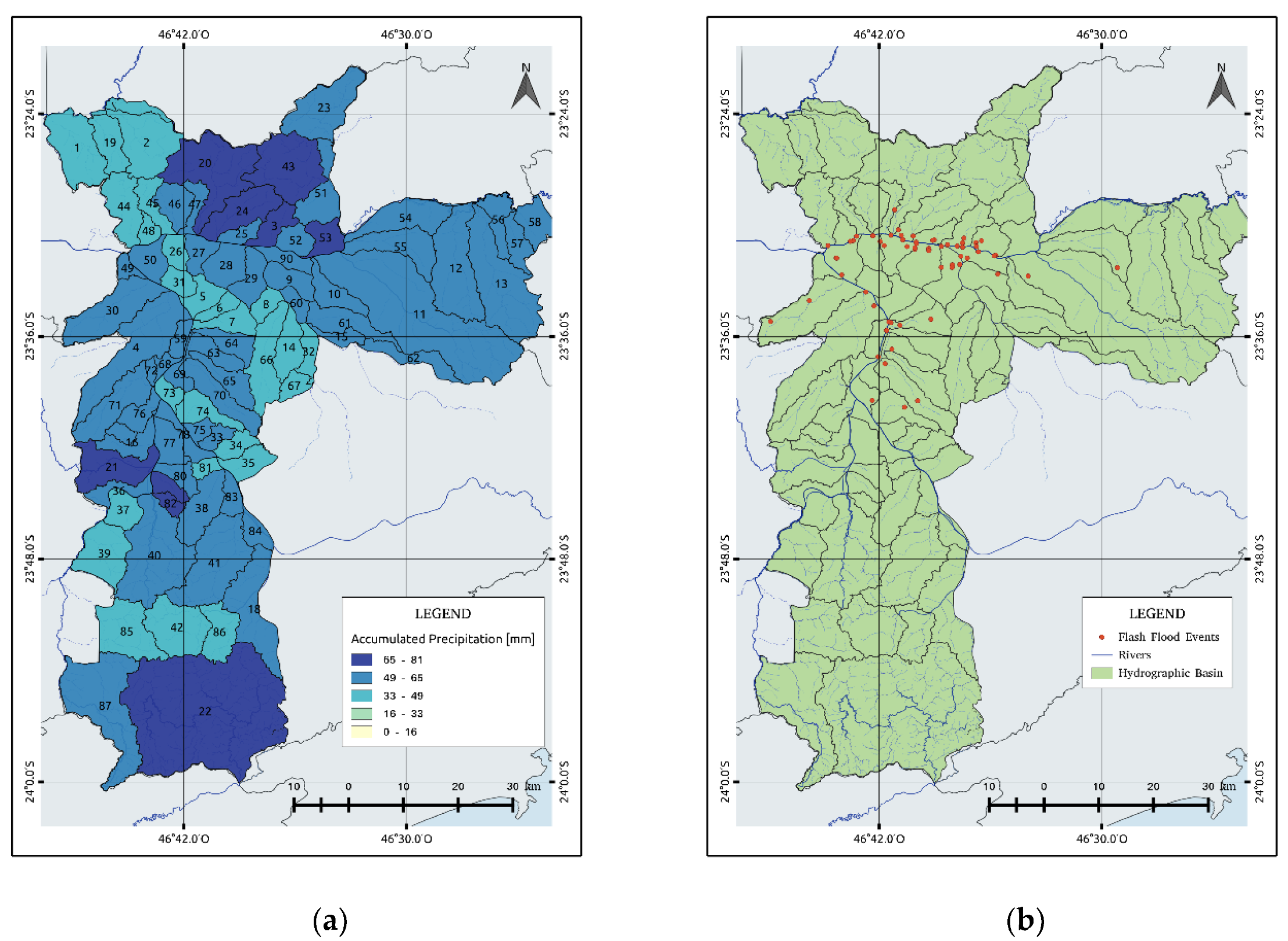
Figure 8a shows the 24-h accumulated rainfall on 11 March 2016. The dark areas represent the watersheds that registered up to 65 to 81 mm of accumulated rainfall.
Figure 8b shows the location of the flash flood points in the city. Although a greater accumulated precipitation can be observed in the northern and southern areas, the flash flood events were concentrated near the two main rivers due to different relieving soil types. For example, the bordering watersheds, such as those in the north and south, have a declivity of more than 60%, which contributes to flash floods downstream.
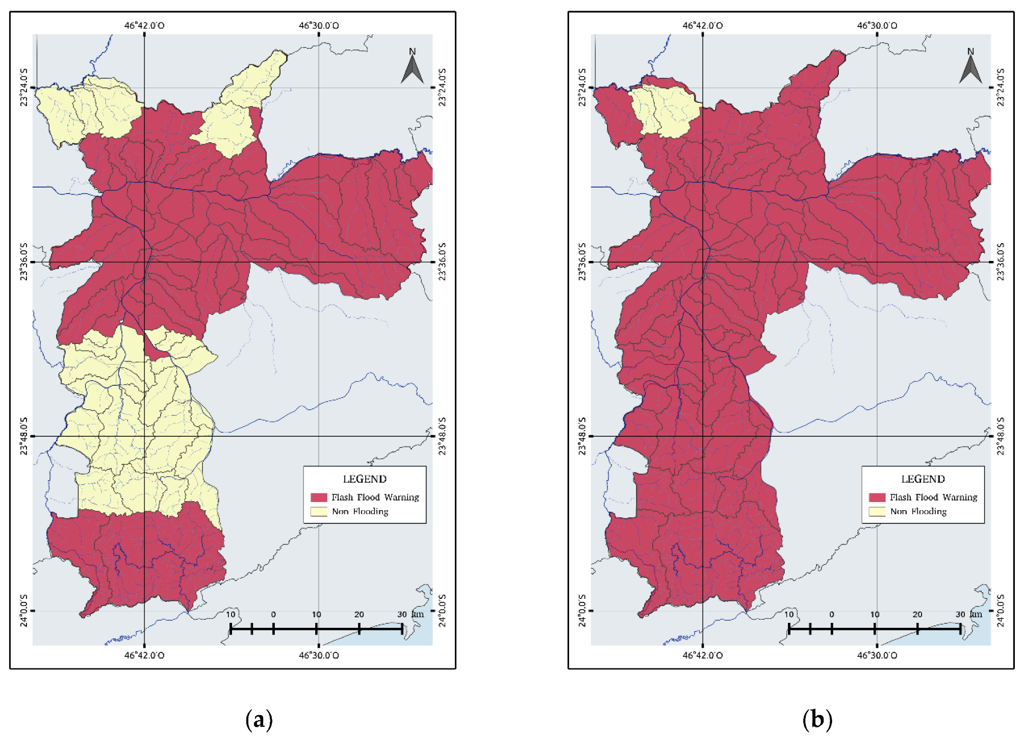
After applying the logistic model, the estimated flash flood warnings were concentrated throughout the city (
Figure 9b) with an exception of two watersheds located in the north. From
Figure 9a,b, it is possible to compare the flash flood warnings related to the flood points observed on that day and the flash flood forecasting, respectively. The logistic regression model generated false alarms in the southern region and a few cases in the north, mainly in the Tremembé and Anhangüera districts. The predictions have an accuracy of 68% and a mean probability of success of 94%. The computed POD reveals that the logistic regression model improves the predictability of flash floods.
4. Conclusions
In our study, we explored the possibility to develop a methodology to forecast flash flood warnings for each watershed using a binary logistic regression model for the city of São Paulo based on the early 24-h rainfall measurements. The model used rain estimates from the dual-polarization S-band Doppler weather radar (SPOL) from the DAEE and the Technological Center of the Hydraulics Foundation (FCTH). The logistic regression model was adjusted to use 24-h accumulated precipitation, a maximum precipitation rate, and rainfall duration for each watershed.
The model presented a mean POD of 0.459 and a mean FAR of 0.12 for flash flood cases. For non-flash flood cases, the POD was 0.954 and the FAR 0.297. When considering only rainy days, the POD for flash flood cases increases to 0.71. These errors indicate that the developed logistic regression model performs better to predict non-flash flood events.
On average, a higher probability of the occurrence of flash flood events was observed in 48% of the watersheds sampled. These watersheds are located in the eastern and central regions near the Tietê and Pinheiros rivers, and the model showed a POD above 50% and a FAR less than 15%. Moreover, the logistic model showed an 86% accuracy in these regions. These regions also registered greater recurrence of flood points that might influence the accuracy of the model.
In general, the capacity of the binary logistic regression model shows an acceptable probability for flash flood occurrence in a certain number of watersheds, while the probability for non-occurrence of flash flood has a better success rate.
