Atmospheric Trace Metal Deposition from Natural and Anthropogenic Sources in Western Australia

Abstract

Aerosols from Western Australia supply micronutrient trace elements including Fe into the western shelf of Australia and further afield into the Southern and Indian Oceans. However, regional observations of atmospheric trace metal deposition are limited. Here, we applied a series of leaching experiments followed by total analysis of bulk aerosol samples to a unique time-series of aerosol samples collected in Western Australia to determine atmospheric concentrations and solubilities of Fe and V, Mn, Co, Zn, and Pb. Positive matrix factorisation analysis indicated that mineral dust, biomass burning particulates, sea salt, and industrial emissions were the major types of aerosols. Overall, natural sources dominated Fe deposition. Higher atmospheric concentrations of mineral dust (sixfold) and biomass burning emissions were observed in warmer compared to cooler months. The fraction of labile Fe (0.6–6.0%) was lower than that reported for other regions of Australia. Bushfire emissions are a temporary source of labile Fe and may cause a peak in the delivery of its more easily available forms to the ocean. Increased labile Fe deposition may result in higher ocean productivity in regions where Fe is limiting, and the effect of aerosol deposition on ocean productivity in this region requires further study.

1. Introduction

Marine biota play a key role in modulating the Earth’s climate through uptake of atmospheric carbon dioxide (CO₂) [1]. Their metabolism, though, is limited by insufficient amounts of trace metals (TMs) in many remote ocean regions [2,3,4,5]. Iron (Fe), for example, limits the growth of marine biota in some parts of the Southern Ocean and the Equatorial and North Pacific. Atmospheric aerosol deposition is a source of Fe and other TMs to open ocean phytoplankton [6,7,8,9,10,11]. Most Fe in the atmosphere is in the mineral form and originates from the upper continental crust [10]. However, this form of Fe is only slightly soluble (~1–2%) and, consequently, only a small percentage may be consumed by marine biota after deposition [12,13]. A wide range of Fe solubilities (<1–90%) has been reported for aerosols worldwide [14]. This variability can be explained by the following: (i) atmospheric processing of mineral dust during transport; (ii) mixing of mineral dust with emissions from more soluble sources, which increases the Fe solubility via averaging or solubilisation of mineral dust during transport; and (iii) methodological differences in the leaching protocol applied for quantification by different laboratories [15]. To date, it is recognized that aerosols from combustion processes contain the most soluble forms of trace metals [16,17,18,19]. Consequently, combustion emissions are important contributors to the global aerosol trace metal (TM) budget, despite their lower contribution to total TM concentrations in the atmosphere. Extensive areas of land are burned each year in some world regions, providing highly fertile aerosols to the land and ocean via atmospheric deposition [20]. Iron solubilities observed for aerosols containing bushfire emissions range from 0.5% to 45% [21,22]. Some aerosol deposition models indicate this type of aerosol source is responsible for up to 50% of total soluble Fe deposited to low nutrients low chlorophyll regions [23]. Besides natural sources, anthropogenic activities produce a wide range of aerosols, such as urban particles and emissions from coal and oil combustion. Iron solubility in these emissions varies from 3% in urban samples to 0.5–25% in coal combustion emissions to as much as 36–81% for oil combustion [24]. It is generally accepted that TMs contained in anthropogenic emissions and biomass burning emissions are more soluble than TMs contained in mineral dust. Therefore, fractional TM solubilities have been reported to be positively correlated with an enrichment of anthropogenic elements in the atmosphere [13,16,25].

Australia contributes 5.6% of global mineral dust emissions [26]. Arid and semi-arid inland areas of Australia, such as the vast Lake Eyre Basin (1.200 million km²) and Murray-Darling Basin (1.061 million km²), contain several active mineral dust sources [27,28]. Analysis of air mass pathways indicates that these mineral dust plumes are transported to the oceans around Australia, including the Southern Ocean, the Indian Ocean the Tasman Sea, and the Coral Sea [19,27,29,30]. In addition, northern regions of Australia are subject to bushfires from spring to autumn, which burn thousands of square kilometres each year, making them responsible for 10.8% of global biomass burned area and around 7.5% of burned biomass globally [20]. Severe bushfires are also common in southern regions of the country under dry, hot, and windy conditions of the warmer months [31,32,33]. Finally, Australia’s largest cities and industries, as well as intensive shipping activities along the coast, are important sources of anthropogenic emissions and contribute to the total atmospheric TM budgets [34,35,36,37,38]. The south-west part of Australia—where both sampling sites (Gingin and Garden Island (GI)) are located—is relatively isolated from urban areas, including the state’s capital Perth, and surrounded by arid and semi-arid land to the east, the Indian Ocean to the west, and the Southern Ocean further south (Figure 1). The surrounding terrain was expected to be a significant source of mineral dust with only minor influences from anthropogenic emissions from the city and suburbs emitted by vehicles, domestic heating, power plants, and ship emissions. Bushfires are also common in the south-west part of Western Australia, where the capital is located, especially during the hotter seasons.

Seasonal temperature and rainfall variations are expected to cause a drop in atmospheric concentrations of natural emissions of dust and bushfires in this region of Australia [39]. At the same time, increased emissions from domestic heating (partially from firewood [40,41]) and coal-fired power plants, located approximately 100 to 250 km south of Gingin, are expected. This may lead to an increase in Fe solubility and enrichment of elements that originate from fossil fuel combustion. Both Gingin and GI sites lie in the path of aerosols transported from Western Australia to the Indian Ocean and SO. Atmospheric Fe deposition to those oceans could potentially cause a biological response by fertilizing plankton growth, particularly in summer [42]. The Southern Ocean is the high nutrient-low-chlorophyll (HNLC), region where Fe is the factor limiting or co-limiting photosynthesis [43,44]. On the other hand, the northeast shelf of Australia (part of IO) is an oligotrophic area, with Fe-limited cyanobacteria responsible for nitrogen fixation [42,45].

Despite being such an important source of aerosols, Australia remains rather poorly studied in terms of potential bioactive trace metals (BATMs), which are key elements in various biochemical processes after deposition to the ocean. Atmospheric deposition on Australia’s west coast in particular is understudied, despite the fact that the second largest Australian dust flux passes over the region before reaching the Indian Ocean and the Southern Ocean [27,28]. To the best of our knowledge, there have been no reported field observations of soluble and total TMs along the coast of Western Australia. The aim of this work is to provide new observations on atmospheric deposition of iron (Fe), vanadium (V), manganese (Mn), cobalt (Co), zinc (Zn), and lead (Pb) in Western Australia. Seasonal data on their atmospheric concentrations in the total and labile (as an indicator of the potential bioavailable forms) fractions were presented and compared with the seasonal variations in activity of main sources of aerosols in the region: mineral dust sources, bushfire emissions, and anthropogenic emissions. The source apportionment results from tracer analysis were compared to the statistical method of positive matrix factorisation (PMF) (supported by data on soluble major ions and total content of barium (Ba), lanthanum (La), cerium (Ce), and uranium (U)). Finally, observed atmospheric concentrations of labile and total fractions of Fe were compared with existing data and estimates from global dust deposition models.

2. Experiments

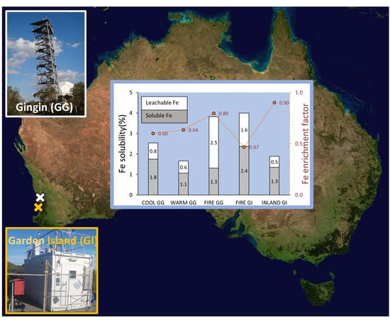
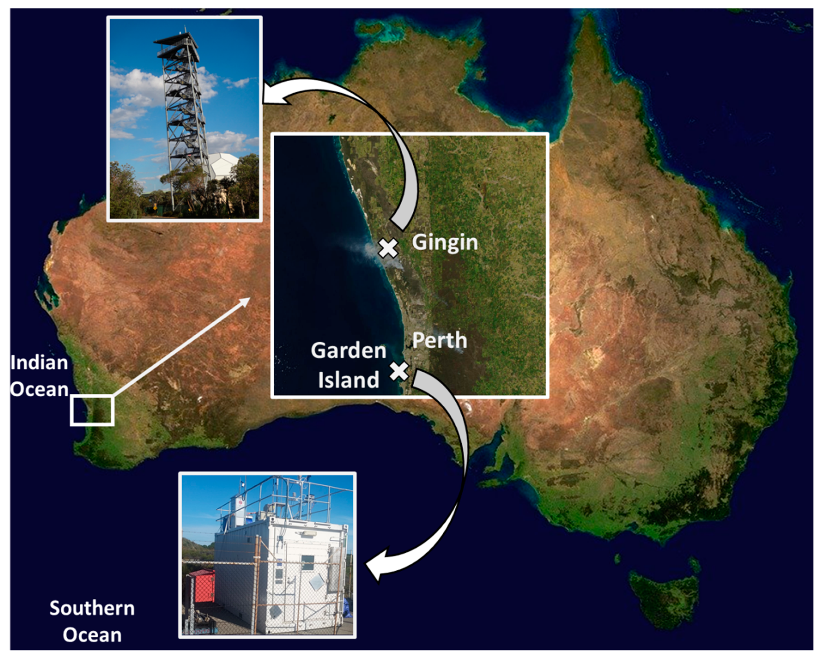
2.1. Study Site and Sample Collection

An aerosol sampling station was established in 2015 at the Gravity Discovery Centre near Gingin (GG), Western Australia, to study the seasonality of atmospheric TM deposition and provenance. The sampler at Gingin was located on the top platform of the 45-meter-high Leaning Tower of Gingin (31.35° S, 115.71° E) (Figure 1), 95 meters above sea level (45 m tower height + land elevation). This location is surrounded by bush, approximately 20 km from the Indian Ocean coastline. A total of 19 samples (sampling period was 5–13 days per sample) and 2 procedural blanks (PB) collected at Gingin were analysed (Table S1). Samples were chosen in cool and warm months to investigate seasonal variations. In addition to these samples, two samples were collected containing bushfire emissions (FIRE GG 1 and FIRE GG 2), which occurred in the Gnangara-Moore River State Forest, <10 km south west from the Gingin sampling site.

In addition, an aerosol sampling campaign was performed on Garden Island (GI) at the Royal Australian Navy base, Western Australia, during the Atmospheric Integrated Research on Burdens and OXidative capacity (AIRBOX) fieldwork ‘Near Sea Surface Aerosol characterization’ in April-May 2018. The HiVol aerosol sampler on GI was located on the roof of the AIRBOX container (32.19° S, 115.68° E, 15 m a.s.l.) near the local gravel road and beach (Figure 1). A total of four samples (sampling period was 1–4 days per sample) and two procedural blanks collected at GI were analysed (Table S1). Similar to Gingin, two samples containing fresh bushfire emissions were also collected (FIRE GI 1 and FIRE GI 2), which likely contained a mixture of emission from the Mundaring State Forest and Youraling State Forest east of Perth and from smaller regional bushfires near the shoreline. Two more samples collected at GI contained aerosols from inland Western Australia that passed the city of Perth (INLAND GI 1 and INLAND GI 2).

Total suspended particulate (TSP) aerosol samples were collected using a high-volume air sampler (HiVol3000, Ecotech. Aerosols were collected on Whatman 41 full sheet (20 × 25 cm) cellulose filters cleaned for TM deposition [46]. After sampling, filters were folded in half with the aerosol loading facing inward. At Gingin, samples were initially stored in a domestic freezer available at the sampling station at −4 °C, followed by transport to the University of Tasmania (UTAS), where they were stored at −20 °C until analysis. There was no freezer facility for sample storage at the GI site. Therefore, samples were instead frozen upon arrival at the laboratory at UTAS, after returning from fieldwork (~2 weeks after sampling). To avoid sample contamination, all filter handling at Gingin was conducted inside a laminar flow hood (AirClean^® AC632LF, Labsystems Group). Filters were touched only using pre-cleaned plastic tweezers. At GI, filter changeovers were conducted inside a ‘clean-box’—a simple in-house-made plastic construction made of polyvinyl chloride pipes and plastic sheeting, inside a car boot because no clean laboratory was available.

Two soil samples were collected at the Gingin site in the proximity of the aerosol sampler. They were collected using a plastic spoon, placed in a double plastic zip-lock bag, and stored at −20 °C. Before analysis, they were sieved using 63 μm stainless steel sieves, to separate the fine fraction, which may undergo suspension into the atmosphere and consequently form aerosols [47]. The fraction below 63 μm was used for inductively coupled plasma mass spectrometry (ICP-MS) analysis and its chemical composition was compared to global averaged values and values of aerosols collected in Gingin to study enrichment factors.

2.2. Trace Metal Analysis

At the University of Tasmania, the entire filter sheets were divided into subsamples using a pre-cleaned circular titanium punch (47 mm) inside an International Organization for Standardization (ISO) class 6 clean room laboratory. The subsamples were treated following a three-step leaching protocol with subsequent analysis by inductively coupled plasma mass spectrometry (ICP-MS) [15]. The protocol consisted of the following three steps conducted consecutively on each subsample to determine soluble, leachable, and refractory fractions. Step 1: The soluble fraction was determined by leaching with 50 mL of ultra-pure water (UPW) passed through the subsample. The filtration set consisted of a Savillex perfluoroalkoxy (PFA) filter holder connected to a Teflon container (for extract collection) and vacuum pump. An aliquot of the UPW leach (9.8 mL) was collected and acidified to 0.14 mol L⁻¹ with distilled HNO₃. Step 2: The leachable fraction was determined by placing the wet filter in a bath of 1.1 M ammonium acetate buffer for 1 h after step 1. The leachate was agitated three times: at the beginning, after 20 min, and after 40 min. To separate remaining particles of the filter, samples were then centrifuged for five minutes. The top 4.5 mL of solution was then pipetted into 15 mL Savillex PFA vials. Samples were dried then re-suspended in 4.5 mL 0.14 mol L⁻¹ HNO₃, and finally transferred into 10 mL auto sampler tubes for analysis. Step 3: The refractory fraction was determined by total digestion of the dried filter remaining after step 2, in a mixture of 1.0 mL of distilled nitric acid (HNO₃) and 0.25 mL of hydrofluoric acid (HF) (SEASTAR, BASELINE^®) at 120 °C for 12 h. Then, samples were evaporated and digested in 5 mL of 7 mol L⁻¹ HNO₃ at 120 °C for 12 h. Once the filter was digested, the samples were evaporated to dryness, re-suspended in 1.4 mol L⁻¹ HNO₃, and diluted to 0.28 mol L⁻¹ HNO₃ solution for analysis. In the following, the sum of soluble (step 1) and leachable (step 2) fractions is termed the ‘labile fraction’, while the sum of all three fractions is termed the ‘total’.

All samples from the above-described protocol were analysed for TM concentrations using ICP-MS, Thermo Element 2, in the Central Science Laboratory, University of Tasmania. The following isotopes were measured to determine elemental concentrations: ²⁷Al, ⁴⁷Ti, ⁵¹V, ⁵²Cr, ⁵⁵Mn, ⁵⁶Fe, ⁵⁹Co, ⁶³Cu, ⁶⁶Zn, ¹³⁸Ba, ¹³⁹La, ¹⁴⁰Ce, ²³⁸U, and ²⁰⁸Pb. The method analytical parameters such as blank contribution and method precision are provided in Appendix A. Instrument parameters and a detailed method description are reported in Perron et al. [15].

2.3. Major Ion Analysis

A 47 mm diameter punch of the W41 cellulose filter was placed into a 10 mL glass container. Following, 8 mL UPW was added and the samples were agitated for 50 min in an ultrasonic bath. Finally, the samples were filtered through 0.22 μm pore size, 33 mm polyethersulfone (PES, sterile, syringe-driven membrane filters (Millipore Express^®) to remove particulates from the extract. The samples were analysed by ion chromatography with a conductivity detector (Dionex ICS 3000) at the Australian Centre for Research on Separation Science (ACROSS) at UTAS. An isocratic flow of 24 mM hydroxide was used as eluent through an AS18 (2 × 250 mm) column for anion separation. Cation separation was achieved using an isocratic gradient of 3–15 mM, with methane sulphonic acid used as an eluent through a CS12A (2 × 250 mm) column. This ‘soluble major ion’ fraction was determined for the following species: Na⁺, NH₄⁺, K⁺, Mg²⁺, Ca²⁺, Cl⁻, NO₃⁻, SO₄²⁻, PO₄³⁻, and C₂O₄²⁻.

Mixed calibration standards were prepared using single element 1000 mg L⁻¹ standards (TraceCERT Sigma Aldrich, Darmstadt, Germany) for all ions except oxalate. The latter was prepared by dissolving di-sodium oxalate (>99.5%, ACS reagent, Sigma-Aldrich 223433), in UPW. In addition to concentrations of ions determined directly, concentrations of non-sea salt sulfate [nss-SO₄²⁻] and non-sea-salt potassium (nss-K⁺) were determined using Equations (1) and (2), respectively:

[nss-SO₄²⁻] = [SO₄²⁻] − [Na⁺] × 0.253

(1)

where [SO₄²⁻] and [Na⁺] indicate atmospheric mass concentrations of SO₄²⁻ and Na⁺, respectively, and 0.253 is the mass ratio between SO₄²⁻ and Na⁺ mass content in sea spray [48].

[nss-K⁺] = [K⁺] − [Na⁺] × 0.0370

(2)

where [K⁺] and [Na⁺] indicate atmospheric mass concentrations of K⁺ and Na⁺, respectively, and 0.0370 is the mass ratio between K⁺ and Na⁺ in sea spray [48].

2.4. Back Trajectories and Burned Area Analysis

To find the origin and transport path of collected aerosols, we used back trajectories generated using the hybrid single particle lagrangian integrated trajectory (HYSPLIT) and global data assimilation system (GDAS0p5) dispersion model from National Oceanic and Atmospheric Administration (NOAA) Air Resources Laboratory (Figure S1) [49,50]. However, owing to the long sampling period at Gingin, aerosols from multiple directions and multiple sources were collected. Therefore, samples were not classified based on the origin from the air masses transport paths. To localise fire events occurring around the sampling site, we used burnt area maps generated weekly by the moderate resolution imaging spectroradiometer ‘MODIS FAA weekly’ model provided by the Western Australian Land Information Authority [51]. Bushfire occurrence was confirmed by satellite images [52]. On the basis of burnt map analysis, samples were divided based on the occurrence of bushfires around the sampling station (more details in Section 3.1).

2.5. Aerosols Sources by Positive Matrix Factorisation

Positive matrix factorisation (PMF) [53] using United States Environmental Protection Agency (EPA) software PMF version 5.0.14 [54] was performed on the matrix of samples by chemical species concentrations to identify potential sources of elements. This implementation of PMF was used because it explicitly incorporates analytical uncertainties and detection limits and provides comprehensive diagnostics of PMF model fits [54]. The samples from Garden Island were excluded owing to missing data and different locations. The following chemical species were included into PMF analysis: total content of metals measured by ICP-MS: Al, Ti, V, Cr, Mn, Fe, Co, Cu, Zn, Ba, La, Ce, U, and Pb; and soluble major ions measured by ion chromatography: Na⁺, NH₄⁺, K⁺, nss-K⁺, Mg²⁺, Ca²⁺, Cl⁻, SO₄²⁻, nss-SO₄²⁻, C₂O₄²⁻, and NO₃⁻. The concentrations of NH₄⁺, Cu, and Cr were down weighted because there were concerns about data quality (Cu and Cr, see.

Table A1. Contribution of procedural blank to determined atmospheric trace elements concentrations. Values above 25% were classified as not satisfactory (red font), values above 10% are bolded. Abbreviated samples codes applied: samples collected during WARM season were labelled as ‘W’, samples collected in COOL season were labelled as ‘C’, and FIRE GG samples were labelled as F. For example, W1 represents sample WARM 1. Data for soluble, leachable, refractory and total fractions were provided for bioactive trace metals (BATMs), for which solubility trends were investigated, while only the total fraction was provided for elements used in positive matrix factorisation (PMF) analysis.

	Sample Code
	W1	W2	W3	W4	W5	W6	U1	C1	C2	C3	C4	C5	C6	C7	C8	F1	F2	W7	U2
soluble
Al	1	1	1	1	2	1	2	16	3	4	9	6	2	9	2	1	0	1	1
Ti	2	1	1	1	6	3	13	10	5	4	23	4	4	6	2	2	1	1	2
V	0	0	0	0	0	0	0	0	0	0	0	0	0	0	0	0	0	0	0
Mn	0	0	0	0	0	0	0	0	0	0	0	0	0	0	0	0	0	0	0
Fe	0	0	0	0	1	0	1	3	1	1	3	2	1	3	1	0	0	0	0
Co	0	0	0	0	0	0	1	9	1	1	4	1	1	3	0	0	0	0	1
Zn	1	0	1	0	1	0	1	1	1	0	3	0	0	1	0	0	0	1	0
Pb	0	0	0	0	0	0	0	0	0	0	0	0	0	0	0	0	0	0	0
leachable
Al	1	1	2	1	1	2	6	24	7	5	26	10	6	13	5	1	1	1	3
Ti	3	4	22	5	10	6	31	35	31	10	48	15	7	19	8	4	2	2	3
V	0	0	1	0	0	0	0	1	1	0	1	0	0	0	0	0	0	0	0
Mn	0	0	0	0	0	0	0	1	0	1	1	1	0	1	0	0	0	0	0
Fe	1	1	3	1	2	2	4	16	7	3	22	5	3	9	2	0	0	1	2
Co	0	0	1	0	0	1	2	10	2	1	8	2	2	1	1	0	0	1	2
Zn	4	3	7	2	3	2	5	6	5	3	18	5	4	8	6	2	3	3	7
Pb	0	0	0	0	0	0	0	1	0	0	1	0	0	1	0	0	0	0	0
refractory
Al	0	0	0	0	0	0	0	13	1	1	2	2	1	2	0	0	0	0	0
Ti	0	0	0	0	0	0	0	5	1	0	2	1	1	1	0	0	0	0	0
V	0	0	0	0	0	0	0	10	1	1	2	1	1	1	0	0	0	0	0
Mn	0	0	0	0	0	0	1	5	1	1	2	2	1	2	0	0	0	0	1
Fe	0	0	0	0	0	0	0	7	1	0	2	1	1	2	0	0	0	0	0
Co	1	1	1	1	1	1	3	36	5	2	12	8	4	4	2	1	1	1	2
Zn	5	3	10	4	4	4	15	78	26	7	35	11	35	20	7	2	4	8	9
Pb	0	0	0	0	0	0	1	7	1	0	2	1	2	1	0	0	0	0	0
total
Al	0	0	0	0	0	0	0	13	1	1	2	2	1	2	0	0	0	0	0
Ti	0	0	0	0	0	0	0	5	1	0	2	1	1	1	0	0	0	0	0
V	0	0	0	0	0	0	0	4	1	0	2	1	1	1	0	0	0	0	0
Cr	2	1	3	1	2	2	5	40	11	4	27	11	11	15	2	0	1	2	4
Mn	0	0	0	0	0	0	1	2	1	0	1	1	1	1	0	0	0	0	0
Fe	0	0	0	0	0	0	0	7	1	0	2	1	1	2	0	0	0	0	0
Co	1	1	1	0	1	1	3	28	4	2	11	4	3	3	1	0	0	1	2
Cu	8	4	20	5	7	6	18	53	24	10	52	39	14	39	9	3	3	6	16
Zn	4	2	7	2	3	2	6	13	7	3	21	5	6	11	4	2	2	4	5
Ba	1	0	1	1	0	1	3	13	5	2	12	8	3	8	2	0	0	1	2
La	0	0	0	0	0	0	0	3	0	0	1	1	1	1	0	0	0	0	0
Ce	0	0	0	0	0	0	0	5	0	0	2	1	1	1	0	0	0	0	0
U	0	0	0	0	0	0	1	4	1	1	2	1	1	1	0	0	0	0	0
Pb	0	0	0	0	0	0	1	1	0	0	1	0	1	1	0	0	0	0	0

) and these elements were poorly modelled in initial model runs (NH₄⁺, Cu, Cr). Four-, five-, and six-factor solutions were explored, but the five- and six-factor solutions did not increase the interpretability of the resulting factors, and the five-factor solution was less stable than the other solutions. For parsimony, the four-factor solution was chosen using 50 random starts. The best-fit four-factor model was assessed for robustness using displacement error estimation (to assess rotational ambiguity of the final solution) and bootstrapped error estimation (to detect and estimate disproportionate effects of small blocks of observations on the final solution). For the bootstrapping, 100 resamples were performed using a block size of two sets. No substantial problems emerged from these diagnostics for the final, four-factor solution.

2.6. Other Calculations

Pearson’s correlation coefficient (r) and scatterplots were used to check for and quantify linear relationships between variables. The following nomenclature for |r| was used: 0.00–0.19 very weak, 0.20–0.39 weak, 0.40–0.59 moderate, 0.60–0.79 strong, and 0.80–1.0 very strong [55]. Correlation coefficients were compared to the Pearson critical value for significance level p = 0.05 to test whether observed correlations were significant.

The enrichment is expressed as the enrichment factor (EF) and shows the scale of anthropogenic derived aerosol in selected elements compared with global upper crustal values. Briefly, the ratio of the concentration of an element (here, [Z]) to the concentration of a mineral dust tracer (here, [Ti]) in aerosols is compared to the ratio of mean global values for upper crustal materials [56] using Equation (3).

EF_Z = ([Z]/[Ti])_aerosol/([Z]/[Ti])_crust

(3)

3. Results and Discussion

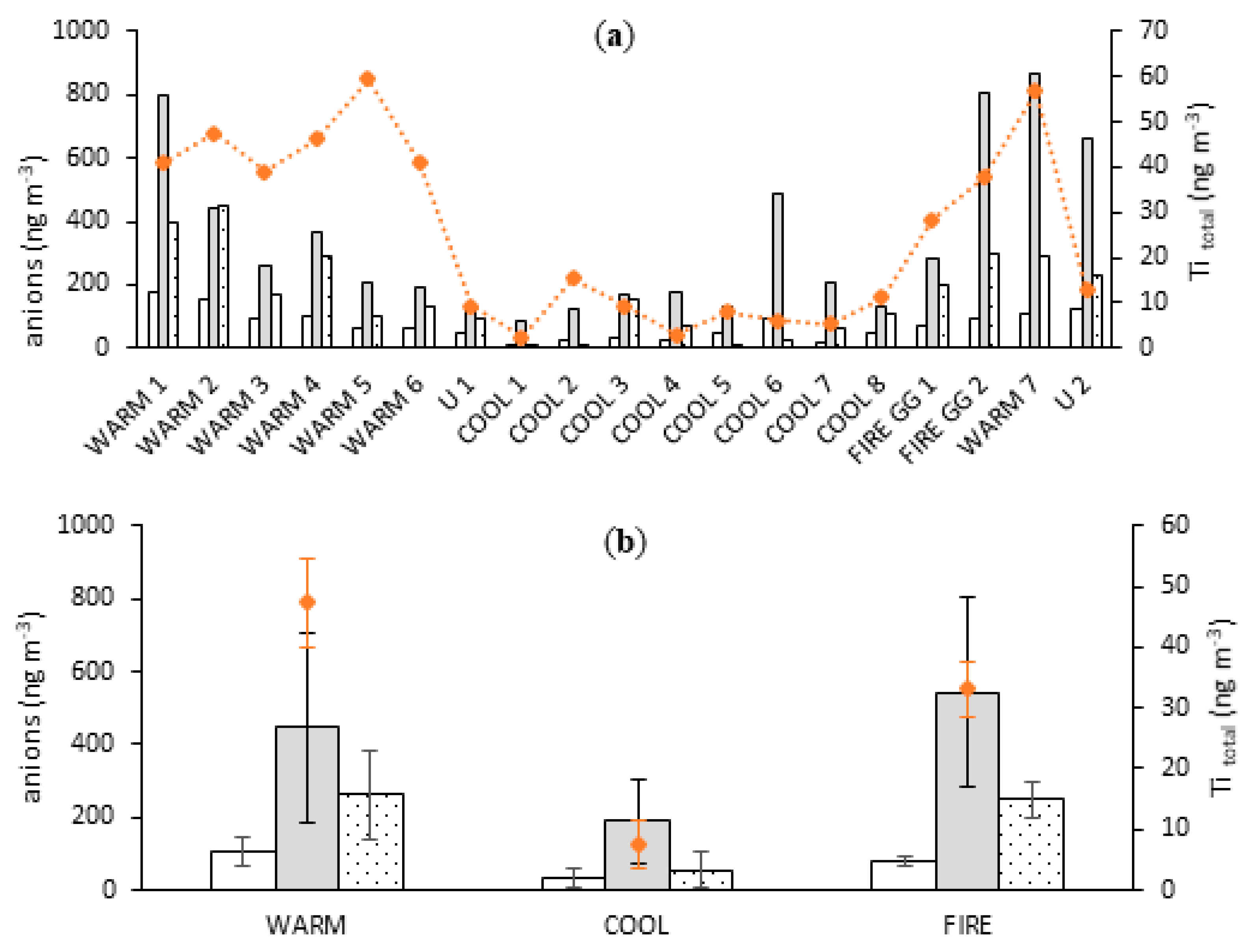
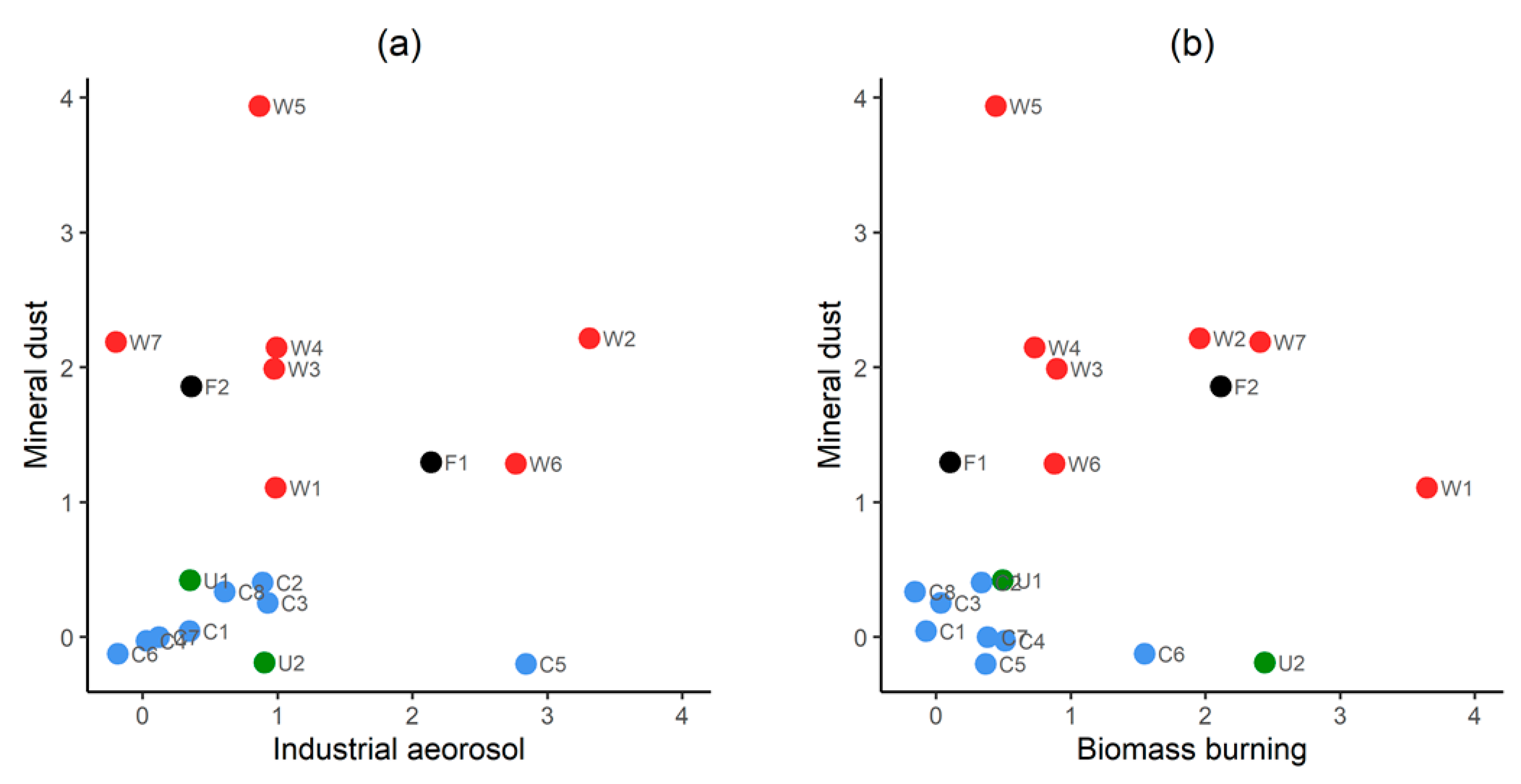
3.1. Seasonality in Aerosol Provenance: Sample Classification

Owing to the long sampling periods at the Gingin site, samples contained aerosols from multiple directions and sources according to wind direction records and air mass pathways (backward trajectories). Therefore, they could not be divided according to air mass origin. Instead, they were divided according to the atmospheric concentration of Ti (as a tracer of mineral dust) (Figure 2) and bushfire occurrence around the sampling site. There were three types of samples, characterised by the following: (i) low mineral dust concentrations (below 20 ng m⁻³ Ti) and minor or no bushfire occurrence within 200 km of the sampling station; (ii) high mineral dust concentrations (above 20 ng m⁻³ Ti) and bushfire occurrence within 200 km from the sampling site, but not in close proximity (<10 km); and (iii) enriched contribution of bushfires due to proximity (<10 km) and/or intensity of bushfire emissions. To simplify nomenclature, in the following text, these types were referred to as COOL (i), WARM (ii), and FIRE GG (iii). The majority of COOL samples were collected during winter 2016, only sample COOL 7 was collected in the late winter to early spring 2015 period. Similarly, most of the WARM samples were collected during autumn with one sample collected in summer 2017 (WARM 6), and one sample was collected in early winter 2015 (WARM 6). Low atmospheric concentrations of Ti accompanied by bushfires recorded within 200 km from the sampling site were observed for two samples. Consequently, these two samples were not assigned to any of the groups and were labelled as U-1 and U-2, respectively. A sample list including assigned sample classification, period of sampling, and corrected volume of filtered air is presented in Table S1.

The average total Ti atmospheric concentration was ~6 times higher for samples collected in WARM compared with COOL conditions, 47 and 8 ng m⁻³, respectively (Figure 2). Atmospheric concentrations of soluble major ions were investigated to assess contributions of bushfire emission and other combustion processes. Soluble forms of nitrate, sulfate, and oxalate were selected as tracers of combustion processes, which most probably originate from bushfire events. Oxidation of precursor gases, SO₂ and NO_x, provides nitric and sulfuric acid to the atmosphere. These precursors originate from combustion processes or oxidation of dimethyl sulphide outgassed to the atmosphere from the sea-surface water [57], or from fossil fuel combustion and biomass burning [58]. Oxalate has multiple sources including, but not limited to motor vehicle emission [59,60], biomass burning [61], and oxidation of acetone and ethylene in the atmosphere [62]. Mean atmospheric concentrations of non-sea-salt sulfate (nss-SO₄²⁻), nitrate (NO₃⁻), and oxalate (C₂O₄²⁻) were higher by 2.4, 4.7, and 3.0 times, respectively, in WARM than in COOL seasons (Figure 2). This likely indicates higher emissions from bushfires and/or more intensive vehicle traffic owing to tourist activities during the WARM period. On the other hand, oxalate, nitrate, and nss-sulfate are all positively correlated (p < 0.05) with the mineral dust tracer, Ti, giving Pearson correlation coefficients of 0.62, 0.67, and 0.48, respectively, suggesting significant contents of major ions species in mineral dust. However, source apportionment by PMF (described in detail in Section 3.5) revealed that none of oxalate, nitrate, and nss-sulfate significantly contributed the mineral dust factor. Instead, this factor contains only 16% of oxalate and below 1% of nss-sulfate and nitrate.

3.2. Mineral Dust Contribution to Atmospheric Trace Metal Deposition

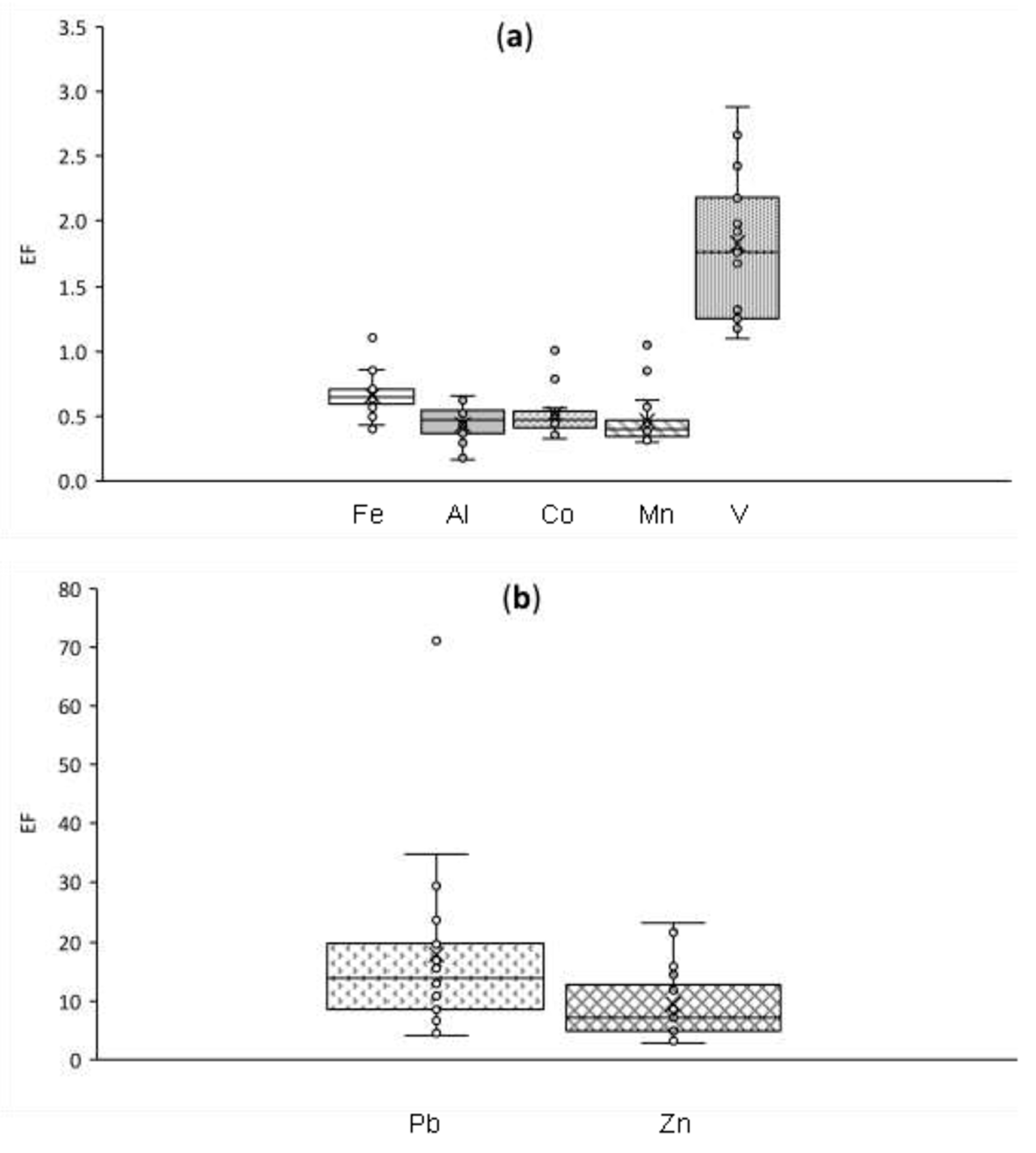
3.2.1. Enrichment Factors

Enrichment factors of BATMs were calculated using Equation (1). On the basis of EF values (

Table 1. Median enrichment factors and Pearson correlation coefficients (r) between atmospheric concentrations of Fe, Co, Mn, Pb, V, Zn, and mineral dust markers (Al, Ti). EF_{soil 1} and EF_{soil 2} show the enrichment of local soils relative to the global upper crustal values [56]. N indicates number of aerosol samples included in this correlation. EF, enrichment factor.

Element	N	rAl	rTi	EFaerosols	EFsoil 1	EFsoil 2
Al	19	1.00	0.98	0.5	0.9	0.6
Ti	19	0.98	1.00	1	1.0	1.0
V	17	0.91	0.92	1.8	3.1	0.6
Mn	17	0.93	0.91	0.4	0.1	0.1
Fe	17	0.98	0.98	0.6	2.9	0.4
Co	16	0.98	0.98	0.5	0.1	0.1
Zn	19	0.67	0.77	7.2	0.4	1.6
Pb	18	0.52	0.62	14.0	0.6	1.5

), BATMs were classified according to their origin following previous studies [63,64]. Crustal elements had the lowest median values of EF, which were 0.5, 0.4, 0.6, and 0.5 for Al, Mn, Fe, and Co, respectively (Table 1). The enrichment factor for V (EF_V) was 1.8, which is higher than that for Mn and Al, but still below 2. Higher EF_V than values of EF_Mn, EF_Fe, and EF_Co may be explained by variability of soil composition, but also by anthropogenic contributions such as ship emissions [65]. Finally, the median EF_Pb was 15.0 and the median EF_Zn was 9.5. Therefore, these two elements were classified as originating from anthropogenic activities.

Values below 1.0 observed for crustal elements indicate that collected aerosols contain mineral dust depleted in those elements compared with the averaged upper continental crust. However, the chemical composition of local soils from Gingin may differ in relation to global averages. Therefore, in order to verify the low EF values of crustal elements in collected aerosols, two local soils (the fraction <63 µm) were analysed by ICP-MS. Soils were digested by the same procedure as aerosol samples. One of the samples was a red soil commonly used as material for unsealed roads in Western Australia, including those in proximity to Gingin (Soil 1). The second soil sample was a local brown/orange soil (Soil 2). The EFs of elements in local soils were then re-calculated as per aerosols using Equation (3), but with local soil values in the numerator and the global averaged upper crust values in denominator. Consequently, this equation provides information on whether local soils are depleted in some elements, and consequently may be responsible for low EF of aerosols collected.

Both local soils had low enrichment factors of Co and Mn (~0.1). This is much less than the median value of aerosols EF_Mn and EF_Co of 0.4 and 0.5, respectively. Sample Soil 1 had the EF_Al of 0.9 and EF_Fe of 2.9, which is higher than the median EF for aerosols of 0.5 and 0.6, respectively. Conversely, Soil 2 had lower EF_Al than Soil 1, at 0.6 and 0.9, respectively. EF_Fe was lower for Soil 2 than Soil 1, at 0.4 and 2.9, respectively. Soil 1 contained elevated EF_V (3.1), while local Soil 2 had elevated EF_Zn (1.6) and EF_Pb (1.5). To summarise, some local soils of Western Australia may be responsible for particularly low EF_Mn and EF_Co in collected aerosols. Findings for EF_Al and EF_Fe indicate variability in the elemental composition of local soils. It is worth noting that only two local soils were analysed in this study. Therefore, these results do not provide representative data for wide range of complex soils in Western Australia. These results indicate only a possible explanation of low EF for certain crustal elements.

3.2.2. Correlation with Mineral Dust Markers

Total aluminium (Al) and total titanium (Ti) are commonly used as mineral dust tracers as their contents in soils are high and relatively constant worldwide. Therefore, the correlations between their atmospheric concentration and the atmospheric concentration of crustal elements are expected to be close to linear. This general trend was observed during the EF analysis, where elements of lower EF were well correlated with mineral dust tracers (Table 1). The correlation between Fe and Co with both mineral dust tracers was very strong (r = 0.98) and significant (p < 0.05). The correlation was slightly lower, but still very strong (r = 0.93) and significant (p < 0.05) between Mn and Al, and between Mn and Ti (r = 0.91). High and significant (p < 0.05) correlation coefficients were observed between V and Al (r = 0.91) and between V and Ti (r = 0.92), which confirms an apparent contribution of crustal materials to total V content. The correlation of anthropogenic elements with mineral dust tracers was weaker than crustal elements. Significant (p < 0.05) correlations were observed between Pb and Al (r = 0.52) and Ti (r = 0.62), and between Zn and Al (r = 0.67) and Ti (r = 0.77).

3.2.3. Iron Enrichment of Australian Aerosols and Soils

Reddish Australian soils (and consequently mineral dust) contain a higher proportion of Fe compared with global average values [66,67,68]. The ratio between Fe and Al (Fe/Al) in aerosols collected in Australia is higher (0.8–1.0) than for aerosols collected in the Northern Hemisphere (0.4–0.5) [66,67,68]. These observations were confirmed by higher enrichments of Fe (EF_Fe = 0.88–1.28) than Al (EF_Al = 0.55–0.76) in aerosols collected in Gunn Point, Northern Territory, Australia [63]. Here, the ratio of Fe/Al for samples collected at Gingin varied between 0.42 and 1.11 (mean of 0.66), which confirms that Australian mineral dust is enriched in Fe, but is also highly heterogeneous. The ratio of Fe/Al was higher within samples collected at Gingin in the COOL season than in the WARM season (0.82 and 0.49, respectively). Local Soil 1 had an Fe/Al ratio of 1.32, while local Soil 2 had a ratio of 0.29. The first value was for the red soil sample taken from the roadside of unsealed road in proximity of the sampling station. Thus, this soil entrained to the atmosphere may enrich Fe in aerosols collected at Gingin. Consequently, the proportion of elements (Fe/Al) in aerosol samples from this source may be higher in the COOL season because of lower mineral dust contributions from remote inland deserts. Another explanation for the higher Fe/Al ratio in the COOL season compared with the WARM season is a higher contribution of anthropogenic emissions from Perth during winter. Previous studies have shown a high ratio of Fe/Al for aerosols collected around large cities. Recalculation of median values from the long-term seasonal observation of PM_2.5 in the Sydney suburb of Liverpool revealed an Fe/Al ratio of 3.7 [36], while the Fe/Al ratio was 1.56 in the Sydney suburb of Richmond [34]. Fresh bushfire samples collected at Gingin and GI had an Fe/Al ratio similar to the rest of the samples collected in this study. Therefore, bushfire emissions did not alter the Fe/Al ratio.

3.3. Seasonality in Bioactive Trace Metal Solubilities and Enrichment Factors

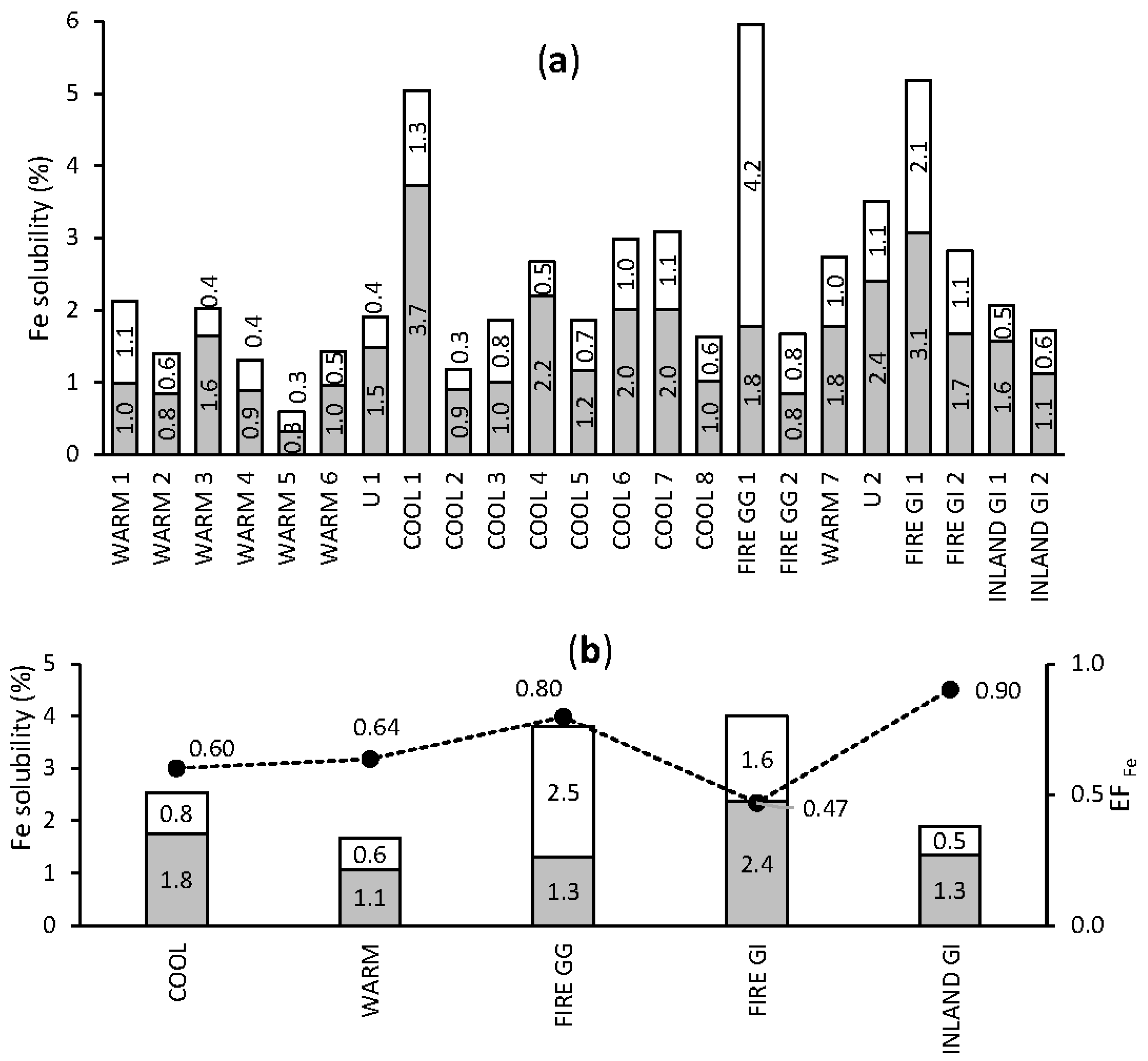
3.3.1. Iron

Fractional Fe solubility (FFeS) results for individual samples and for groups are shown in Figure 3. Overall, the soluble fraction of Fe contributed 0.3–3.7% (mean 1.5%) to total Fe. The leachable Fe comprised 0.4–4.2% (mean 0.9%) of total Fe. Consequently, the labile fraction contributed 0.6–6.0% (mean 2.5%) of total Fe and the majority of the labile fraction (mean 64.0%) was in the soluble form. The bushfire emission sample FIRE GG 1 was an exception, where the soluble fraction (1.8%) was lower than the leachable fraction (4.2%). However, for all other samples containing elevated bushfire emissions, the soluble Fe fraction was equal to (FIRE GG 2) or higher than (FIRE GI 1 and FIRE GI 2) the leachable Fe fraction.

The mean FFeS was slightly higher for COOL samples compared with WARM samples, at 2.6 and 1.7%, respectively. There was also a slight shift in median EF_Fe, which was higher for the samples collected in WARM than in COOL seasons, at 0.64 and 0.60, respectively. A higher FFeS was observed in aerosol containing fresh bushfire emissions from both Gingin and GI sites, where the labile Fe fraction contributed 3.8 and 4.0% of total Fe, respectively. The Fe solubility reported here is lower than reported for aerosols collected along the south and north sector of Western Australia’s coast, where the fraction of labile Fe ranged from 7% to 16% (median 8%) and from 3% to 15% (median 5%), respectively [69]. However, aerosols analysed by Perron et al. [69] were collected at sea on a research vessel, while aerosols analysed here were collected on land. Therefore, the former may be expected to contain a smaller fraction of coarse particulates (which have been deposited before reaching the ocean), which mainly consisted of poorly soluble mineral forms of Fe. Current models predict an atmospheric Fe solubility between 6% and 8% of total Fe in Western Australia [70], significantly higher than the mean labile Fe of 2.5% observed for all our samples, and higher than the seasonal means. To evaluate the possible overestimation of Fe solubility in the study region by the current models (particularly in winter), further ship-based studies are required.

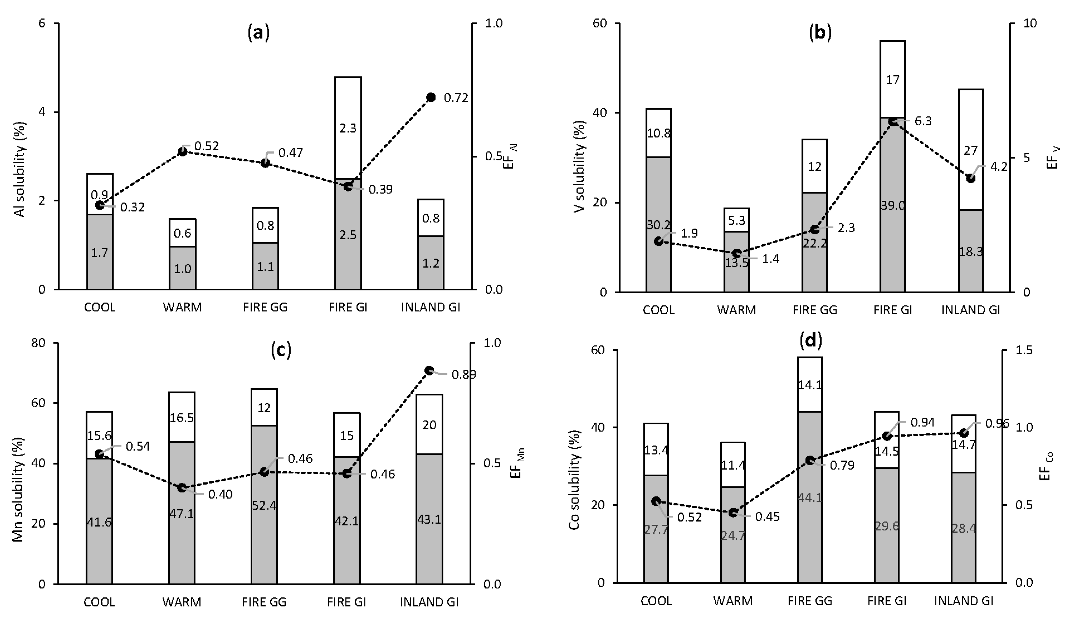
3.3.2. Crustal and Mixed Origin Elements: Al, V, Mn, and Co

Seasonal trends in the solubility and EF of crustal and mixed origin elements are presented in Figure 4. The seasonal trend of Al was similar to Fe: COOL aerosol samples contained more soluble Al compared with WARM samples. The seasonal mean of the labile fraction of Al was 2.6% and 1.6%, while the seasonal mean EF_Al values were 0.32 and 0.52 for COOL and WARM samples, respectively. Within each group, the fraction of soluble Al was higher than the fraction of leachable Al. The mean solubility of the labile Al fraction of FIRE samples from Gingin was 1.9%, falling between the mean values for WARM and COOL samples. In contrast, Al solubility of FIRE GI samples was 4.8% of the labile fraction in total, more than two times the mean for INLAND GI samples (2.0%). The solubility trend of Co was aligned to Fe and Al, with aerosols collected in COOL season containing slightly more soluble Co than those collected in WARM season, 41.1% versus 36.1% of total Co. The EF_Co was slightly higher in the COOL than in WARM season (0.52 and 0.45). Samples FIRE GG had the highest fractional Co solubility, while the samples FIRE GI had levels similar to INLAND GI samples. Soluble forms contributed the majority of the labile Co fraction. Manganese was the only crustal element for which higher solubility was observed for the WARM group than for the COOL group, (63.6% and 57.2% of labile fraction, respectively). FIRE GG samples contained more soluble forms of Mn than samples collected in WARM season. Bushfire smoke collected at GI contained 57.1% of Mn in labile form, similar to the mean value of COOL samples. Variation in V solubility was analogous to that reported for Al, Fe, and Co, meaning aerosols collected in WARM season contained, as a mean, a lower proportion of labile V (to total V) than those collected in COOL season, 18.8% and 41.0%, respectively. Enrichment factor of V was lower in WARM season than in COOL season, (1.5 and 1.9, respectively). Nevertheless, the highest EF_V (2.3) among samples collected at Gingin was observed for FIRE GG samples. Similar results were observed for samples collected at GI, where EF_V was higher for FIRE GI than INLAND GI samples, (6.3 and 4.2, respectively). The much higher EF_V of samples from GI than from Gingin may be explained by the closer distance of GI to Perth and to Fremantle marine port, as both are potential sources of anthropogenic V.

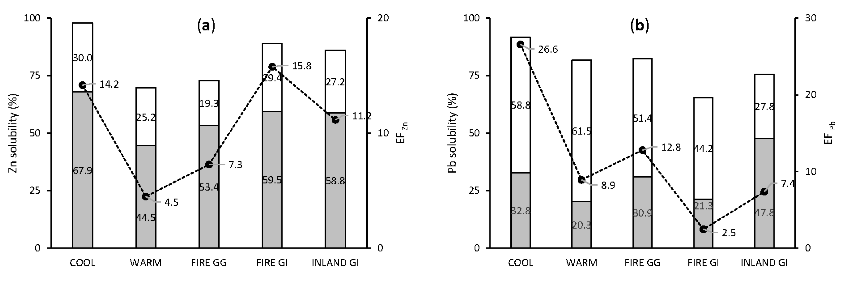
3.3.3. Anthropogenic Elements: Pb and Zn

Solubilities and EFs of anthropogenic elements were slightly higher in aerosols collected in COOL than in WARM season (Figure 5). The mean labile fraction of Pb was 91.6% and 81.8% of total Pb in COOL and WARM season, respectively. A greater (as a proportion) difference was observed for EF, which, for Pb, was (as mean) of 26.6 in COOL season and 8.9 in WARM season. Lead was the only element for which the leachable fraction was the dominant fraction. This agrees with observations from Morton et al. [46], who reported that the ammonium acetate leach dissolved between 36% and 98% of total Pb, about 10 times more than other extraction mediums. The labile fraction of Pb in FIRE GG samples was close to those collected in COOL and WARM season, while the labile fraction of Pb in FIRE GI samples was even lower than samples without bushfire emission (INLAND GI). This indicates that bushfires were not a source of additional soluble Pb. The EF_Pb of aerosols from GI was lower than for aerosols from Gingin. Garden Island is isolated from the mainland, and consequently may have lower Pb soil contamination from vehicle emissions, which historically used petrol containing Pb. Similar to Pb, labile fraction of Zn and EF_Zn were higher in COOL season (labile Zn = 97.9%, EF_Zn = 14.2) than in WARM season (labile Zn = 69.7%, EF_Zn = 4.5). These observations confirmed that anthropogenic activities provided additional soluble Zn in COOL conditions. The solubilities observed for FIRE GG and FIRE GI samples were close to the rest of the samples, suggesting a lack of noticeable flux of soluble Zn from bushfires.

3.4. Sources of Soluble and Leachable Bioactive Trace Metals at Gingin Site

3.4.1. Solubility as a Function of EFs

It is generally accepted that anthropogenic emissions contain more soluble forms of TMs than mineral dust [16,17,24]. Therefore, to explore this link, correlations between fractional solubilities and EFs for single sample measurements at Gingin were studied (Figure S2). Samples from GI were not included in the correlation because they were collected in a different location and there were only four samples (two FIRE GI samples and two INLAND GI samples) analysed—too few for statistical analysis at this station. The results for aerosols collected at Gingin revealed a correlation between fractional solubility of soluble (r = 0.803), leachable (r = 0.606), and labile (r = 0.789) fractions of V with EF_V. Similarly, the soluble and labile fractions of Zn were correlated with EF_Zn, (r = 0.768 and 0.726, respectively). Vanadium was classified as being of mixed origin, predominantly crustal, with possible contribution from anthropogenic sources, while Zn was classified as predominantly anthropogenic. This shows that contribution of both anthropogenic and crustal sources of total V and Zn play important roles by influencing fractional solubility of these metals. The leachable and labile fractions of Co increased with increasing EF_Co, (r = 0.712 and 0.726, respectively). Finally, the percentage of labile Pb correlated with EF_Pb (r = 0.8), while there was no significant correlation for separate soluble and leachable fractions of Pb. There was no significant correlation between EF and the solubility of Al, Mn, and Fe. All these elements were classified as crustal (low EF and very good correlation with mineral dust tracers). Therefore, their contribution from anthropogenic sources to total content of these elements was probably negligible.

Anthropogenic emissions were tested as a source of soluble and leachable forms of Fe in the next step. Correlation between FFeS (soluble and leachable) with total content of anthropogenic (Pb and Zn) and mixed origin (V) elements was determined to evaluate the anthropogenic contribution to soluble and leachable forms of Fe. In addition to anthropogenic sources, these elements are contained in the upper crust. Therefore, to eliminate Zn and Pb sourced from crust, their atmospheric content was normalised to a mineral dust tracer (Ti). A significant (p < 0.05) moderate correlation was observed between percent of soluble and leachable Fe with V/Ti (r = 0.484 and r = 0.523) and with Zn/Ti (r = 0.589 and r = 0.523). On the other hand, no significant correlation between soluble Fe and Pb/Ti, V/Ti, and Zn/Ti was found when aerosols collected in COOL and WARM seasons were considered separately. Fraction of leachable forms of Fe (%) were strongly (r = 0.739) correlated with Zn/Ti in COOL season. This indicates that anthropogenic sources provided leachable forms of Fe in COOL conditions, whereas leachable Fe was strongly and significantly correlated (r = 0.819) with V/Ti in WARM season. No significant correlation between soluble and leachable Fe and Pb/Ti was found in any of the analysed groups. According to the results, despite being a minor source of total Fe, anthropogenic emission provided a noticeable proportion of leachable Fe, particularly in some seasons.

3.4.2. Fractional Iron Solubility as a Function of Soluble Major Ions

An impact of bushfire emission and acidic processes in the atmosphere on FFeS was studied. The soluble form of nss-K⁺ normalised to total Ti and soluble oxalate were tested as potential tracers of biomass burning. Normalisation of nss-K⁺ to total Ti was applied to exclude the contribution from soluble K from mineral sources. Globally, the concentration of oxalate over the urban area has been reported to be higher than over the remote and rural areas [61,71]. The mean (±SD) oxalate concentration in the atmosphere in this study was 73 ± 46 ng m⁻³, similar to results reported in remote/rural areas of Australia rather than to urban areas [61]. The mean (±SD) atmospheric concentration of oxalate was higher for WARM than for COOL group (109±40 and 36±27 respectively) (Figure 2). This indicates the seasonal patterns of oxalate and which has been reported to remote/rural areas (but not in urban areas). In this study, variation may be particularly caused by contribution of fire emissions and temperature variations, which agrees with the seasonal cycle of oxalate reported in several places in Australia [61]. However, in this study, oxalate is strongly (r = 0.617) correlated with mineral dust (significant for p < 0.05); this may be explained by a resuspension of oxalate absorbed on upper crust materials.

No relationship was observed between both potential tracers (nss-K⁺ and oxalate) within a group of all samples and among samples collected in WARM and COOL season separately. This is contrary to observations of Gillett et al. [61], who found a very strong correlation (R² = 0.975) between nss-K⁺ and oxalate for samples containing smog from large forest fire burning east and north east of Melbourne in December 2006 to January 2007. A lack of analogical correlation among WARM samples may be explained by a reduced bushfire contribution to total collected aerosol owing to the (in most cases) remote bushfire location and long sampling periods. As the consequence of the second reason, the contribution of bushfire emission in total collected aerosols was not strong enough to be observed in this way.

As the next step, nss-K⁺ and oxalate concentrations were correlated with soluble major ions (NO₃⁻, nss-SO₄²⁻, NH₄⁺) emitted mainly by combustion processes. There was no correlation between nss-K⁺/Ti_total with any of the mentioned species among groups of all samples and within the WARM and COOL groups. On the other hand, oxalate was strongly and significantly correlated with NO₃⁻ and nss-SO₄²⁻ within all samples, with correlation coefficients of 0.858 and 0.786, respectively. Oxalate was also strongly correlated with nss-SO₄²⁻ (r = 0.840) within the COOL group and with nitrate (r = 0.939) within WARM group. Positive correlations with mentioned soluble major ions suggest that oxalate is more appropriate (than nss-K⁺) as a tracer of combustion processes at Gingin. These results agree with the studies of Zhou et al. [71] in Hong Kong, where oxalate was correlated with nss-SO₄²⁻ and NO₃⁻ and the strongest correlation was observed in summer. Experiments in combustion chambers revealed rather constant K⁺/SO₄²⁻ ratio in combustion emission from different types of biomass [72]. Consequently, a lack of correlations between nss-K⁺ and acidic species may also suggest a significant contribution of sources other than biomass burning to the nss-K⁺ budget.

Finally, the correlation between FFeS and soluble major ions was determined. For all samples, the Pearson’s correlation coefficient between percent of soluble Fe with nss-K⁺/Ti _total, nss-SO₄²⁻/Ti _total, and NH₄⁺/Ti_total was strong and significant, at 0.616, 0.614, and 0.787 respectively. Stronger correlations were observed within the COOL group, where soluble Fe correlations with nss-K⁺/Ti _total reached 0.865, while with NH₄⁺/Ti _total, it reached 0.960—both correlations were significant. Within the WARM group, only nss-SO₄²⁻/Ti _total and percent of leachable Fe were significantly and positively correlated (r = 0.976), which is similar to observations from Tsukuba (Japan), where Fe solubility was related to existing in sulfate forms [73]. No significant correlation was found between FFeS and oxalate atmospheric concentration, itself, and divided by Ti, in any of the analysed groups. This may be explained by the multiple sources of these species, including biomass burning, vehicle exhaust, and atmospheric processes such as oxidation of acetylene and ethylene.

Surprisingly, a strong correlation between FFeS and nss-K⁺/Ti was observed for COOL group aerosols. Because no bushfires were observed at this time, the relationship may be explained by significant contributions of K⁺ emitted from the coal combustion. Coal-fired power plants emit K and may contribute large proportions of nss-K⁺ in industrial and urban areas, making nss-K⁺ an unreliable marker of biomass burning [74]. The sampling station at Gingin lies approximately 100 km north of the nearest big coal power plant, Kwinana (640 MW), and approximately 250 km north from a complex of power plants including Muja (845 MW), Bluewaters (416 MW), Collie (300 MW), and Worsley Alumina (107 MW). Back trajectories indicate air masses frequently passed over the region of the coal power plants before reaching the Gingin site. Lead was reported to be enriched in fly ash from coal combustion [75,76]. In this study, a higher EF_Pb was observed during COOL than WARM season, 26.6 and 8.9, respectively, supporting this hypothesis.

Overall, the data presented here show that the application of tracers for bushfires in this region is challenging. Oxalate patterns align with NO₃⁻ and nss-SO₄²⁻, but are not correlated with FFeS. This is against findings from Section 3.3.1, which showed that samples that contained emissions from bushfires contain more labile Fe than others. This may be explained by the relatively low contribution of bushfire emissions to the labile Fe fraction compared with mineral dust. In addition, nss-K⁺ does not correlate with either oxalate, NO₃⁻, and nss-SO₄²⁻, and appears to be a poor tracer of bushfires emission. Its correlation with FFeS may be explained by a coincident signal from local coal-fired power plants.

3.4.3. Fractional Iron Solubility as a Function of Mineral Dust Tracer Solubility

The aim of this part of the study was to evaluate the proportion of soluble and leachable forms of BATM provided by mineral dust sources. Thus, correlations between soluble and leachable forms of BATM and soluble, leachable, and total forms of Al were studied (Figure S3). Aluminium was chosen as the mineral dust tracer because Ti is much less abundant and less soluble, which induces much higher measurement error. The highest (>0.8) correlations were observed for Co and Mn, while for Fe, the Pearson correlation coefficient was slightly below 0.8. These observations confirmed that mineral dust is an important source of both total and potentially bioavailable (more soluble) forms of crustal elements. Lower correlations (between 0.4 and 0.6) were observed between soluble and leachable forms of V. However, the lowest correlations were observed for anthropogenic elements, Pb and Zn, 0.03 and 0.3 for soluble forms and 0.4 and 0.7 in leachable form, respectively. That mean amount of soluble forms of Pb and Zn was rather independent of the mineral dust, while leachable forms are moderately or strongly connected with the mineral dust atmospheric concentration. Soluble and leachable forms of Al and Fe were very strongly and significantly correlated, with correlation coefficients of 0.97 and 0.96, respectively. This indicates that both were released/dissolved from the same matrix. Particulates detected by scanning electron microscopy were mostly alumina-silicates containing high amounts of Fe, possibly as Fe substitutes in crystal lattice of alumina-silicates. High correlations between Co and Al were observed for their soluble and leachable forms (r = 0.727 and r = 0.857) and similarly between soluble and leachable forms of V and Al (r = 0.780 and r = 0.749). On the other hand, a moderate correlation was observed for soluble and leachable Mn and Al (r = 0.489 and r = 0.564). Finally, soluble forms of the anthropogenic elements did not depend on soluble mineral forms. The correlation coefficient between soluble Pb and Al was –0.018, while between Zn and Al, it was 0.317.

A higher correlation was observed between soluble and leachable Fe with soluble and leachable Al than with total Al. This may be explained by temporal variations in more soluble forms of Fe and Al in mineral dust. These variations may be caused by different mineral dust forms and by the fact that both Fe and Al are also contained in products of coal combustion [24] or biomass burning [77]. A lower correlation between soluble and leachable Fe with Co and Mn was observed even though Co, Fe, and Mn are crustal elements. However, Co and Mn are more soluble crustal elements compared with Al. For samples collected at Gingin (outstanding sample FIRE GG 1 excluded), the mean (±SD) fractional solubility for the labile form was higher for Co (40.55% ± 8.96%) and Mn (46.62% ± 5.36%) than for Al (1.88% ± 0.65%) or Fe (2.26% ± 1.23%). Thus, it is more probable that Fe was released from the same matrix as Al (Fe substituted alumina-silicates) than from mineral matrices containing Co and Mn.

Generally, biomass ash is a complex heterogeneous mixture of organic and inorganic matter with fluid phases [78,79]. Inorganic and organic matter consist of amorphous, semi-crystalline, and crystalline (minerals) solids [78,79]. Elements such as Fe, Al, and Mn are contained in biomass and coal ashes as well as mineral dust [78]. Worldwide mean concentrations of Fe in coal ashes are 9.9% and 1.0% in plants ashes; for Al, these values are 11.5% and 1.4%, respectively; while for Mn, they are 0.049% and 0.75% respectively [80]. The chemical composition of ashes from burning of eight biomass samples varied 0.05–0.60% (mean 0.33%) for Al, 0.16–0.74% (mean 0.40%) for Fe, and 0.02–1.06% (mean 0.19%) for Mn [79]. The total content of the elements and their solubilities vary significantly with sources of biomass burning. According to a compilation of data from worldwide results collected and presented by Vassilev et al. [78], biomass ashes contained 0–1% (mean < 0.1%) of soluble Fe, 0–9% (mean 0.9%) of soluble Al, and 0–46% (mean 9.6%) of soluble Mn. Overall, the data presented here show a possible contribution of biomass and fossil fuels ashes to the total and soluble TM budget in aerosols and indicate that combustion processes may be an additional source, next to mineral dust sources of Fe, Al, Mn, and Co, with contributions depending on collected biomass burning emission.

3.5. Sources Identification and Estimation of Their Contribution in Total Collected Aerosols: PMF Analysis

Four types of aerosols were assigned to the factors based on the elements’ contribution in factor profiles (Figure 6): (1) industrial aerosol—with a high contribution of Pb, NH₄⁺, NO₃⁻, and Zn; (2) mineral dust—with a dominant contribution of upper crustal elements such as Al, Ti, Fe, and Ca accompanied by less abundant crustal elements such as Mn, Co, La, Ce, and Ba; (3) sea salt—with a predominant contribution of Mg²⁺, Cl⁻, Ca²⁺, and SO₄²⁻; and (4) biomass burning—characterised by the highest contribution of C₂O₄²⁻, nss-SO₄²⁻, and NO₃⁻. A lack of nss-K⁺ contribution in biomass burning may be explained by other sources contributing the soluble nss-K⁺ pool (see Section 3.4.2).

The samples collected in WARM and COOL conditions were best separated from each other on scatter plots between industrial aerosol versus mineral dust, and between biomass burning versus mineral dust (Figure 7). Concentration of mineral dust is the main separating factor when plotted with industrial emission (Figure 7a), which is consistent with the seasonal variation in total Ti (mineral dust tracer). Sample WARM 5 is an outlier containing the highest concentration of total Ti. Samples WARM 2, WARM 6, COOL 5, and FIRE GG 1 are only samples containing a high contribution of industrial aerosol. However, they do not show a common source and/or land area passed during the airmasses transport according to the backward trajectory analysis. The samples with high industrial signature were collected over a long time-span and were characterised by a wide range of mineral dust concentrations in the atmosphere. Therefore, it is hard to assign them to one specific source, here, we suggest it may be explained by temporal variations in delivery from a major emission source: (i) power plants of Coolie (260 km south), Muja (270 km south), and Blue Waters (260 km south), which together emitted a total of 1100 kg of ammonia and 372.9 kg of Pb and compounds in 2015/2016 [81]. Other potential sources of Pb and ammonia are alumina refineries located in Neerabup (40 km south), Kwinana (100 km south), Pinjarra (150 km south), and Wagerup (170 km south), which emitted to the atmosphere a total of 98,000 kg of ammonia and 133 kg of Pb and compounds in 2015/2016 [81]. Mineral dust and biomass burning factors contributions allow a good separation between COOL and WARM samples (Figure 7b). Two outliers could be explained by the maximum mineral dust concentration (WARM 5) and maximum oxalate concentration (WARM 1). Surprisingly, sample FIRE GG 1 has a low biomass burning factor contribution, despite containing fresh bushfire emissions according to satellite images of the near bushfire event and dark grey filter colour. However, it may be explained by the relatively long sampling period when aerosols without biomass burning contribution were collected and/or by the fact that the pump was off at the end of sampling period and loose particulates from the top of the filter may be removed by wind. In general, the findings from PMF analysis confirm our observations from tracer analysis and interpretation from bulk chemical analysis, indicating that natural aerosol sources dominate TM atmospheric fluxes. Two distinct seasons were observed, which differ in mineral dust and biomass burning loadings.

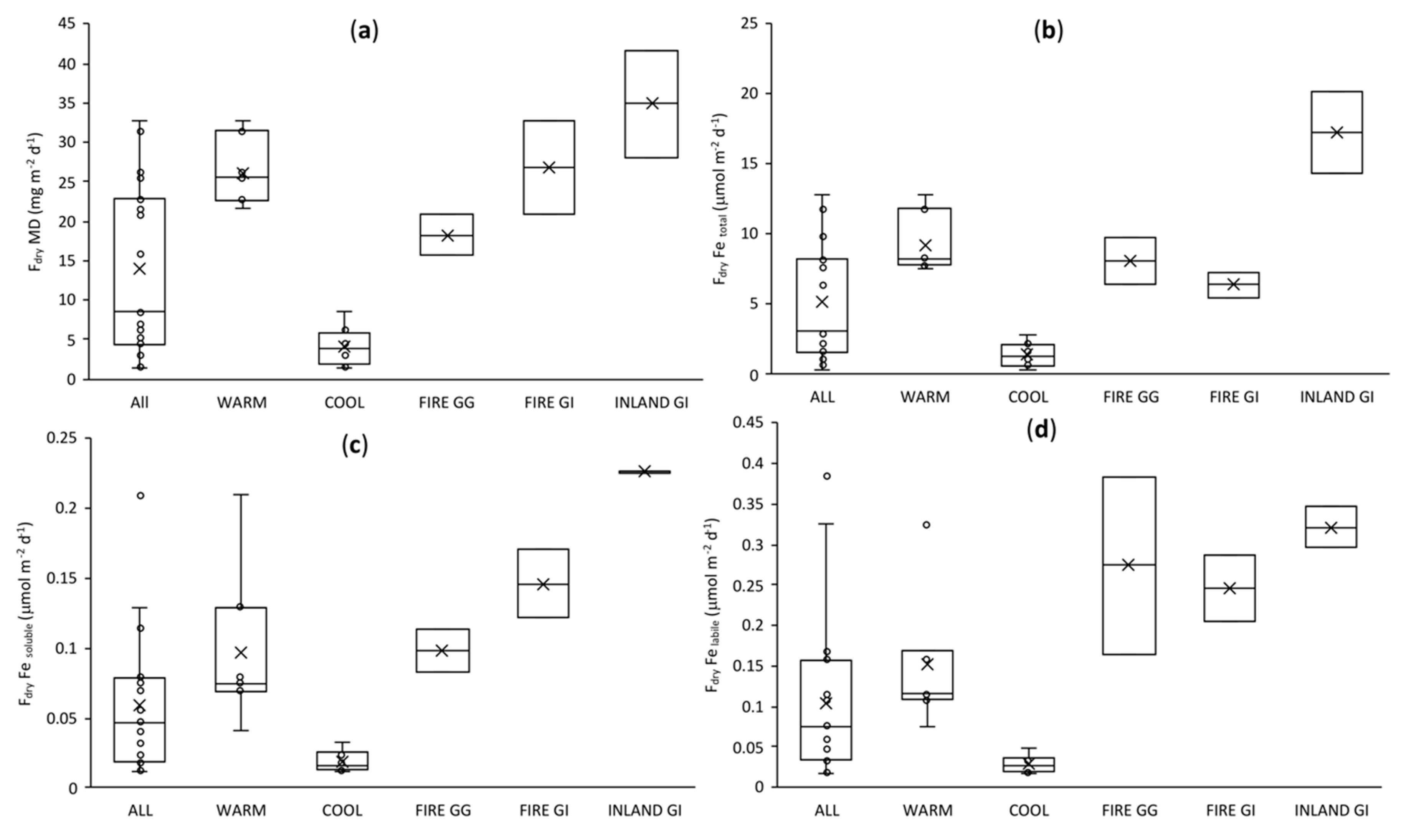
3.6. Dry Deposition Fluxes of Fe: Comparison with Models and Data from Other Regions of Australia

Atmospheric concentrations of total Fe in aerosols collected at Gingin varied between 12 and 418 ng m⁻³ (mean 167 ng Fe m⁻³). A difference of 6.5 times in total Fe concentration between mean values for WARM and COOL groups was observed (300 and 46 ng Fe m⁻³, respectively). This variation is caused by the difference in mineral dust loading variation between COOL and WARM seasons (2.4 and 15 μg m⁻³). These values were calculated based on total Ti atmospheric concentrations and on the global average Ti content in the upper crust of 0.311% [56]. Current models predict atmospheric total Fe concentrations in Western Australia of 100–1000 ng m⁻³ [10]. Our results from in-field measurements (average of 167 ng Fe m⁻³) were within the lower range of these estimates, however, the average of the COOL season (46 ng Fe m⁻³) was well below global model estimates.

The fractional Fe solubility was expressed as the percentage contribution of labile forms (the sum of soluble and leachable forms) of Fe to total Fe. Aerosols collected at Gingin contained 0.6–6.0% (mean 2.4%) of labile Fe. The mean fraction of labile Fe was slightly higher in COOL (2.5%) than WARM (1.7%) season and was the highest (3.8%) for the samples affected by bushfire emissions. In general, the fractions of labile Fe reported here are lower than estimates from models (4–8%) for this part of Australia [70].

On the basis of EF analysis, Fe, Al, Mn, and Co were classified as crustal elements, while V was classified as having a mixed origin. Thus their fluxes were calculated using a coarse particle atmospheric velocity of 2 cm s⁻¹, as recommended for coastal sites by Duce et al. [6] and followed by Winton et al. [63] and Strzelec et al. [82]. Particles emitted by anthropogenic activities are generally in the finer size mode; consequently, the atmospheric velocity may be around an order of magnitude lower [6] than the velocity of crustal elements, thus a velocity of 0.2 cm s⁻¹ was applied to calculate the fluxes of Pb and Zn. It is worth noting the uncertainty due to the high range of reported deposition fluxes (e.g., 10-fold estimated by Duce et al. [6]). Winton et al. [63] and Strzelec et al. [82] assumed an uncertainty in the deposition velocity of up to 50%. Here, we compare seasonal trends in deposition fluxes, and thus estimation of uncertainty is not included. However, for the purpose of further analysis, we recommend to apply a propagation error of 50% of the value of the deposition velocity combined with analytical uncertainties following Winton et al. [63]. Mean (±SD) atmospheric dry deposition fluxes of soluble, labile, and total Fe collected at Gingin were 0.059 ± 0.049, 0.104 ± 0.099, and 5.15 ± 3.97 μmol m⁻² d⁻¹, respectively. Fluxes of soluble and labile Fe are similar to those reported by Perron et al. [69] for southern (soluble Fe: 0.076 ± 0.046 and labile Fe 0.076 ± 0.082 μmol m⁻² d⁻¹) and northern (soluble Fe: 0.043 ± 0.074 and labile Fe: 0.057 ± 0.081 μmol Fe m⁻² d⁻¹) sectors of the Western Australia coast. Meanwhile, fluxes of total Fe reported here are higher than those reported by Perron et al. [69]: 1.02 ± 1.02 and 1.24 ± 90 μmol m⁻² d⁻¹ for southern and northern sector of coastal regions of Western Australia, respectively [69]. The great difference in total Fe fluxes and similarity in soluble and labile Fe fluxes may be explained by the higher contribution of coarse mineral dust particles for land-based (this study) than for ship-based [69] collected samples. Fluxes of total, soluble, and labile Fe were considerably higher in WARM (9.25 ± 2.01, 0.097 ± 0.052, and 0.152 ± 0.083 μmol m⁻² d⁻¹, respectively) than in COOL (1.41 ± 0.83, 0.019 ± 0.007, and 0.029 ± 0.012, respectively) seasons (Figure 8). This has implications for possible ocean atmospheric Fe fertilisation, as the Southern Ocean and the Indian Ocean may be more receptive to fertilisation in the WARM season (more light and warmer waters). Consequently, a higher atmospheric deposition of soluble and labile Fe provides the possibility of a biological ocean response [42]. In addition, high fluxes of soluble and labile Fe (as mean ± SD) were observed in samples containing a greater contribution of bushfire smoke particles, 0.099 ± 0.16 and 0.274 ± 0.110 μmol m⁻² d⁻¹ for FIRE GG samples and 0.146 ± 0.24 and 0.246 ± 0.041 μmol m⁻² d⁻¹ for FIRE GI samples (Figure 8), indicating a high fertilisation potential of bushfire smoke from frequent bushfires along the Western Australia coast, which are also more common in WARM conditions. Dry deposition fluxes of soluble, labile, and total Al, V, Mn, Co, Zn, and Pb calculated for groups of samples collected at Gingin and GI are given in Figure S4.

4. Conclusions

Here, we provided the first seasonal observations on atmospheric TM deposition on the western coast of Australia and revealed the possible overestimation of global aerosol deposition models in terms of Fe solubility. Aerosols were predominantly of natural origin (mineral dust, bushfires, sea salt), reflecting the surrounding landscape, arid land, and low population density. However, the contribution of industrial emissions was noticeable for some samples according to PMF analysis and was a dominant source of Pb and Zn in general. Iron solubility was relatively low (mean 2.5% of labile Fe) compared with other regions of Australia and was rather constant inter-seasonally (mean 1.7% and 2.6% for WARM and COOL season, respectively) despite the high (sixfold) variability in mineral dust content in the atmosphere. The southwestern part of Australia has a lower population and few industrial activities compared with the eastern and southern parts of Australia, where higher Fe solubilities have been reported [69,82]. During the WARM season, aerosols contained an apparent contribution of bushfire emissions in Western Australia, which is an additional source of more soluble Fe. Consequently, delivery of soluble, labile, and total Fe to the waters of either the south-eastern part of the Indian Ocean or the western part of the Southern Ocean is linked to dust and bushfire events across Western Australia, rather than to local anthropogenic activities, which appeared to have a lower contribution. Thus, the activity of mineral dust sources may be a good proxy for either labile or total fluxes of Fe to the ocean, but the fluxes may be temporary perturbated by emissions from bushfires. Anthropogenic emissions most likely from local industries provided a noticeable enrichment of elements such as Zn and Pb, as evidenced by PMF analysis. The supply of these elements needs to be monitored as they may be harmful for nearby marine ecosystems.

References

1. Siegenthaler, U.; Sarmiento, J.L. Atmospheric carbon dioxide and the ocean. Nature 1993, 365, 119–125. [Google Scholar] [CrossRef]
2. Martin, J.H.; Fitzwater, S.E. Iron deficiency limits phytoplankton growth in the north-east Pacific subarctic. Nature 1988, 331, 341–343. [Google Scholar] [CrossRef]
3. Martin, J.H.; Coale, K.H.; Johnson, K.S.; Fitzwater, S.E.; Gordon, R.M.; Tanner, S.J.; Hunter, C.N.; Elrod, V.A.; Nowicki, J.L.; Coley, T.L.; et al. Testing the iron hypothesis in ecosystems of the equatorial Pacific Ocean. Nature 1994, 371, 123–129. [Google Scholar] [CrossRef]
4. Boyd, P.W.; Jickells, T.; Law, C.S.; Blain, S.; Boyle, E.A.; Buesseler, K.O.; Coale, K.H.; Cullen, J.J.; de Baar, H.J.W.; Follows, M.; et al. Mesoscale Iron Enrichment Experiments 1993–2005: Synthesis and Future Directions. Science 2007, 315, 612–617. [Google Scholar] [CrossRef] [Green Version]
5. Moore, C.M.; Mills, M.M.; Arrigo, K.R.; Berman-Frank, I.; Bopp, L.; Boyd, P.W.; Galbraith, E.D.; Geider, R.J.; Guieu, C.; Jaccard, S.L.; et al. Processes and patterns of oceanic nutrient limitation. Nat. Geosci. 2013, 6, 701–710. [Google Scholar] [CrossRef] [Green Version]
6. Duce, R.A. The atmospheric input of trace species to the world ocean. Glob. Biogeochem. Cycles 1991, 5, 193–259. [Google Scholar] [CrossRef]
7. Duce, R.A.; Tindale, N.W. Atmospheric transport of iron and its deposition in the ocean. Limnol. Oceanogr. 1991, 36, 1715–1726. [Google Scholar] [CrossRef]
8. Ussher, S.J.; Achterberg, E.P.; Worsfold, P.J. Marine Biogeochemistry of Iron. Environ. Chem. 2004, 1, 67–80. [Google Scholar] [CrossRef]
9. Jickells, T.D.; An, Z.S.; Andersen, K.K.; Baker, A.R.; Bergametti, G.; Brooks, N.; Cao, J.J.; Boyd, P.W.; Duce, R.A.; Hunter, K.A.; et al. Global Iron Connections Between Desert Dust, Ocean Biogeochemistry, and Climate. Science 2005, 308, 67–71. [Google Scholar] [CrossRef] [Green Version]
10. Mahowald, N.M.; Engelstaedter, S.; Luo, C.; Sealy, A.; Artaxo, P.; Benitez-Nelson, C.; Bonnet, S.; Chen, Y.; Chuang, P.Y.; Cohen, D.; et al. Atmospheric iron deposition: Global distribution, variability, and human perturbations. Annu. Rev. Mar. Sci. 2009, 1, 245–278. [Google Scholar] [CrossRef] [Green Version]
11. Baker, A.R.; Croot, P.L. Atmospheric and marine controls on aerosol iron solubility in seawater. Mar. Chem. 2010, 120, 4–13. [Google Scholar] [CrossRef]
12. Mahowald, N.; Ward, D.S.; Kloster, S.; Flanner, M.G.; Heald, C.L.; Heavens, N.G.; Hess, P.G.; Lamarque, J.-F.; Chuang, P.Y. Aerosol Impacts on Climate and Biogeochemistry. Annu. Rev. Environ. Resour. 2011, 36, 45–74. [Google Scholar] [CrossRef] [Green Version]
13. Sholkovitz, E.R.; Sedwick, P.N.; Church, T.M.; Baker, A.R.; Powell, C.F. Fractional solubility of aerosol iron: Synthesis of a global-scale data set. Geochim. Cosmochim. Acta 2012, 89, 173–189. [Google Scholar] [CrossRef]
14. Scanza, R.A. The Impact of Resolving Mineralogy of Dust on Climate and Biogeochemistry. Ph.D. Thesis, Cornell University, Ann Arbor, MI, USA, 2016. [Google Scholar]
15. Perron, M.M.G.; Strzelec, M.; Gault-Ringold, M.; Proemse, B.C.; Boyd, P.W.; Bowie, A.R. Assessment of leaching protocols to determine the solubility of trace metals in aerosols. Talanta 2020, 208, 120377. [Google Scholar] [CrossRef] [PubMed]
16. Sedwick, P.N.; Sholkovitz, E.R.; Church, T.M. Impact of anthropogenic combustion emissions on the fractional solubility of aerosol iron: Evidence from the Sargasso Sea. Geochem. Geophys. Geosyst. 2007, 8, Q10Q06. [Google Scholar] [CrossRef]
17. Schroth, A.W.; Crusius, J.; Sholkovitz, E.R.; Bostick, B.C. Iron solubility driven by speciation in dust sources to the ocean. Nat. Geosci. 2009, 2, 337–340. [Google Scholar] [CrossRef]
18. Takahashi, Y.; Higashi, M.; Furukawa, T.; Mitsunobu, S. Change of iron species and iron solubility in Asian dust during the long-range transport from western China to Japan. Atmos. Chem. Phys. 2011, 11, 11237–11252. [Google Scholar] [CrossRef] [Green Version]
19. Ito, A. Atmospheric Processing of Combustion Aerosols as a Source of Bioavailable Iron. Environ. Sci. Technol. Lett. 2015, 2, 70–75. [Google Scholar] [CrossRef]
20. Ito, A.; Penner, J.E. Global estimates of biomass burning emissions based on satellite imagery for the year 2000. J. Geophys. Res. D Atmos. 2004, 109, D14S05. [Google Scholar] [CrossRef]
21. Guieu, C.; Bonnet, S.; Wagener, T.; Loÿe-Pilot, M.D. Biomass burning as a source of dissolved iron to the open ocean? Geophys. Res. Lett. 2005, 32, L19608. [Google Scholar] [CrossRef]
22. Paris, R.; Desboeufs, K.V.; Formenti, P.; Nava, S.; Chou, C. Chemical characterisation of iron in dust and biomass burning aerosols during AMMA-SOP0/DABEX: Implication for iron solubility. Atmos. Chem. Phys. 2010, 10, 4273–4282. [Google Scholar] [CrossRef] [Green Version]
23. Luo, C.; Mahowald, N.; Bond, T.; Chuang, P.Y.; Artaxo, P.; Siefert, R.; Chen, Y.; Schauer, J. Combustion iron distribution and deposition. Glob. Biogeochem. Cycles 2008, 22, GB1012. [Google Scholar] [CrossRef]
24. Desboeufs, K.V.; Sofikitis, A.; Losno, R.; Colin, J.L.; Ausset, P. Dissolution and solubility of trace metals from natural and anthropogenic aerosol particulate matter. Chemosphere 2005, 58, 195–203. [Google Scholar] [CrossRef] [PubMed]
25. Chance, R.; Jickells, T.D.; Baker, A.R. Atmospheric trace metal concentrations, solubility and deposition fluxes in remote marine air over the south-east Atlantic. Mar. Chem. 2015, 177, 45–56. [Google Scholar] [CrossRef] [Green Version]
26. Tanaka, T.Y.; Chiba, M. A numerical study of the contributions of dust source regions to the global dust budget. Glob. Planet. Chang. 2006, 52, 88–104. [Google Scholar] [CrossRef]
27. Bowler, J.M. Aridity in Australia: Age, origins and expression in aeolian landforms and sediments. Earth Sci. Rev. 1976, 12, 279–310. [Google Scholar] [CrossRef]
28. Hesse, P.P.; McTainsh, G.H. Australian dust deposits: Modern processes and the Quaternary record. Quat. Sci. Rev. 2003, 22, 2007–2035. [Google Scholar] [CrossRef]
29. Kiefert, L.; McTainsh, G.H. Oxygen isotope abundance in the quartz fraction of aeolian dust: Implications for soil and ocean sediment formation in the Australasian region. Soil Res. 1996, 34, 467–473. [Google Scholar] [CrossRef]
30. Mahowald, N.M.; Baker, A.R.; Bergametti, G.; Brooks, N.; Duce, R.A.; Jickells, T.D.; Kubilay, N.; Prospero, J.M.; Tegen, I. Atmospheric global dust cycle and iron inputs to the ocean. Glob. Biogeochem. Cycles 2005, 19, GB4025. [Google Scholar] [CrossRef]
31. Radhi, M.; Box, M.A.; Box, G.P.; Gupta, P.; Christopher, S.A. Evolution of the optical properties of biomass-burning aerosol during the 2003 southeast Australian bushfires. Appl. Opt. 2009, 48, 1764–1773. [Google Scholar] [CrossRef]
32. Yusiharni, E.; Gilkes, R.J. Changes in the mineralogy and chemistry of a lateritic soil due to a bushfire at Wundowie, Darling Range, Western Australia. Geoderma 2012, 191, 140–150. [Google Scholar] [CrossRef]
33. Duc, H.N.; Chang, L.T.-C.; Azzi, M.; Jiang, N. Smoke aerosols dispersion and transport from the 2013 New South Wales (Australia) bushfires. Environ. Monit. Assess. 2018, 190, 428. [Google Scholar] [CrossRef] [PubMed]
34. Cohen, D.D.; Crawford, J.; Stelcer, E.; Atanacio, A.J. Application of positive matrix factorization, multi-linear engine and back trajectory techniques to the quantification of coal-fired power station pollution in metropolitan Sydney. Atmos. Environ. 2012, 61, 204–211. [Google Scholar] [CrossRef]
35. Cohen, D.D.; Stelcer, E.; Atanacio, A.; Crawford, J. The application of IBA techniques to air pollution source fingerprinting and source apportionment. Nucl. Instrum. Methods Phys. Res. Sect. B 2014, 318, 113–118. [Google Scholar] [CrossRef]
36. Cohen, D.D.; Stelcer, E.; Garton, D.; Crawford, J. Fine particle characterisation, source apportionment and long-range dust transport into the Sydney Basin: A long term study between 1998 and 2009. Atmos. Pollut. Res. 2011, 2, 182–189. [Google Scholar] [CrossRef] [Green Version]
37. Taylor, M.P. Atmospherically deposited trace metals from bulk mineral concentrate port operations. Sci. Total Environ. 2015, 515–516, 143–152. [Google Scholar] [CrossRef]
38. Rate, A.W. Multielement geochemistry identifies the spatial pattern of soil and sediment contamination in an urban parkland, Western Australia. Sci. Total Environ. 2018, 627, 1106–1120. [Google Scholar] [CrossRef]
39. Bureau of Meteorology. Available online: http://www.bom.gov.au/ (accessed on 4 October 2019).
40. Driscoll, D.; Milkovits, G.; Freudenberger, D. Impact and Use of Firewood in Australia; CSIRO Sustainable Ecosystems: Canberra, Australia, 2000. [Google Scholar]
41. Murdoch University. Available online: http://www.see.murdoch.edu.au/resources/info/Res/wood/ (accessed on 24 October 2019).
42. Cropp, R.A.; Gabric, A.J.; Levasseur, M.; McTainsh, G.H.; Bowie, A.; Hassler, C.S.; Law, C.S.; McGowan, H.; Tindale, N.; Viscarra Rossel, R. The likelihood of observing dust-stimulated phytoplankton growth in waters proximal to the Australian continent. J. Mar. Syst. 2013, 117–118, 43–52. [Google Scholar] [CrossRef] [Green Version]
43. de Baar, H.J.W.; de Jong, J.T.M.; Bakker, D.C.E.; Löscher, B.M.; Veth, C.; Bathmann, U.; Smetacek, V. Importance of iron for plankton blooms and carbon dioxide drawdown in the Southern Ocean. Nature 1995, 373, 412–415. [Google Scholar] [CrossRef]
44. Boyd, P.; LaRoche, J.; Gall, M.; Frew, R.; McKay, R.M.L. Role of iron, light, and silicate in controlling algal biomass in subantarctic waters SE of New Zealand. J. Geophys. Res. Ocean. 1999, 104, 13395–13408. [Google Scholar] [CrossRef] [Green Version]
45. Thompson, P.A.; Bonham, P.; Waite, A.M.; Clementson, L.A.; Cherukuru, N.; Hassler, C.; Doblin, M.A. Contrasting oceanographic conditions and phytoplankton communities on the east and west coasts of Australia. Deep Sea Res. Part II Top. Stud. Oceanogr. 2011, 58, 645–663. [Google Scholar] [CrossRef]
46. Morton, P.L.; Landing, W.M.; Hsu, S.C.; Milne, A.; Aguilar-Islas, A.M.; Baker, A.R.; Bowie, A.R.; Buck, C.S.; Gao, Y.; Gichuki, S.; et al. Methods for the sampling and analysis of marine aerosols: Results from the 2008 GEOTRACES aerosol intercalibration experiment. Limnol. Oceanogr. Methods 2013, 11, 62–78. [Google Scholar] [CrossRef] [Green Version]
47. World Atlas of Desertification, 3rd ed.; Cherlet, M.; Hutchinson, C.; Reynolds, J.; Hill, J.; Sommer, S.; von Maltitz, G. (Eds.) Publication Office of the European Union: Luxembourg, 2018. [Google Scholar] [CrossRef]
48. Keene, W.C.; Pszenny, A.A.P.; Galloway, J.N.; Hawley, M.E. Sea-salt corrections and interpretation of constituent ratios in marine precipitation. J. Geophys. Res. Atmos. 1986, 91, 6647–6658. [Google Scholar] [CrossRef]
49. Stein, A.F.; Draxler, R.R.; Rolph, G.D.; Stunder, B.J.B.; Cohen, M.D.; Ngan, F. NOAA’s HYSPLIT Atmospheric Transport and Dispersion Modeling System. Bull. Am. Meteorol. Soc. 2015, 96, 2059–2077. [Google Scholar] [CrossRef]
50. Rolph, G.; Stein, A.; Stunder, B. Real-time Environmental Applications and Display sYstem: READY. Environ. Model. Softw. 2017, 95, 210–228. [Google Scholar] [CrossRef]
51. Landgate Fire Watch. Available online: http://firewatch-pro.landgate.wa.gov.au/home.php (accessed on 4 October 2019).
52. NASA. Available online: https://zoom.earth/ (accessed on 4 October 2019).
53. Paatero, P.; Tapper, U. Positive matrix factorization: A non-negative factor model with optimal utilization of error estimates of data values. Environmetrics 1994, 5, 111–126. [Google Scholar] [CrossRef]
54. Norris, G.; Duvall, R.; Brown, S.; Bai, S. EPA Positive Matrix Factorization (PMF) 5.0 Fundamentals and User Guide. In Guide (User Guide No. EPA/600/R-14/108); U.S. Environmental Protection Agency: Washington, DC, USA, 2014. [Google Scholar]
55. Evans, J.D. Straightforward Statistics for the Behavioral Sciences; Thomson Brooks/Cole Publishing Co.: Belmont, CA, USA, 1996. [Google Scholar]
56. Wedepohl, H.K. The composition of the continental crust. Geochim. Cosmochim. Acta 1995, 59, 1217–1232. [Google Scholar] [CrossRef]
57. Cullis, C.F.; Hirschler, M.M. Atmospheric sulphur: Natural and man-made sources. Atmos. Environ. (1967) 1980, 14, 1263–1278. [Google Scholar] [CrossRef]
58. Galbally, I.; Roy, C.R. The Fate of Nitrogen Compounds in the Stmosphere; Springer: Dordrecht, The Netherlands, 1983; pp. 265–284. [Google Scholar] [CrossRef]
59. Kawamura, K.; Kaplan, I.R. Motor exhaust emissions as a primary source for dicarboxylic acids in Los Angeles ambient air. Environ. Sci. Technol. 1987, 21, 105–110. [Google Scholar] [CrossRef]
60. Chebbi, A.; Carlier, P. Carboxylic acids in the troposphere, occurrence, sources, and sinks: A review. Atmos. Environ. 1996, 30, 4233–4249. [Google Scholar] [CrossRef]
61. Gillett, W.R.; Galbally, I.; Ayers, G.P.; Selleck, P.W.; Jennifer, P.; Meyer, C.P.; Keywood, M.; Fedele, R. Oxalic acid and oxalate in the atmosphere. In Proceedings of the 4th IUAPPA World Congress Clean Air Partnerships: Coming Together for Clean Air, Brisbane, Australia, 9–13 September 2007. [Google Scholar]
62. Warneck, P. In-cloud chemistry opens pathway to the formation of oxalic acid in the marine atmosphere. Atmos. Environ. Atmos. Environ. 2003, 37, 2423–2427. [Google Scholar] [CrossRef]
63. Winton, V.H.L.; Edwards, R.; Bowie, A.R.; Keywood, M.; Williams, A.G.; Chambers, S.; Selleck, P.W.; Desservettaz, M.; Mallet, M.; Paton-Walsh, C. Dry season aerosol iron solubility in tropical northern Australia. Atmos. Chem. Phys. Discuss. 2016, 16, 12829–12848. [Google Scholar] [CrossRef] [Green Version]
64. Buck, C.S.; Aguilar-Islas, A.; Marsay, C.; Kadko, D.; Landing, W.M. Trace element concentrations, elemental ratios, and enrichment factors observed in aerosol samples collected during the US GEOTRACES eastern Pacific Ocean transect (GP16). Chem. Geol. 2019, 511, 212–224. [Google Scholar] [CrossRef] [Green Version]
65. Viana, M.; Amato, F.; Alastuey, A.; Querol, X.; Moreno, T.; García Dos Santos, S.; Herce, M.D.; Fernández-Patier, R. Chemical Tracers of Particulate Emissions from Commercial Shipping. Environ. Sci. Technol. 2009, 43, 7472–7477. [Google Scholar] [CrossRef]
66. Radhi, M.; Box, M.A.; Box, G.P.; Keywood, M.D.; Cohen, D.D.; Stelcer, E.; Mitchell, R.M. Size-resolved chemical composition of Australian dust aerosol during winter. Environ. Chem. 2011, 8, 248–262. [Google Scholar] [CrossRef]
67. Radhi, M.; Box, M.A.; Box, G.P.; Mitchell, R.M.; Cohen, D.D.; Stelcer, E.; Keywood, M.D. Size-resolved mass and chemical properties of dust aerosols from Australia’s Lake Eyre Basin. Atmos. Environ. 2010, 44, 3519–3528. [Google Scholar] [CrossRef]
68. Radhi, M.; Box, M.A.; Box, G.P.; Mitchell, R.M.; Cohen, D.D.; Stelcer, E.; Keywood, M.D. Optical, physical and chemical characteristics of Australian continental aerosols: Results from a field experiment. Atmos. Chem. Phys. 2010, 10, 5925–5942. [Google Scholar] [CrossRef] [Green Version]
69. Perron, M.M.G.; Proemse, B.C.; Strzelec, M.; Gault-Ringold, M.; Boyd, P.W.; Sanz Rodriguez, E.; Paull, B.; Bowie, A.R. Origin, transport and deposition of aerosol iron to Australian coastal waters. Atmos. Environ. 2020, 228, 117432. [Google Scholar] [CrossRef]
70. Mahowald, N.M.; Hamilton, D.S.; Mackey, K.R.M.; Moore, J.K.; Baker, A.R.; Scanza, R.A.; Zhang, Y. Aerosol trace metal leaching and impacts on marine microorganisms. Nat. Commun. 2018, 9, 2614. [Google Scholar] [CrossRef]
71. Zhou, Y.; Huang, X.H.H.; Bian, Q.; Griffith, S.M.; Louie, P.K.K.; Yu, J. Sources and atmospheric processes impacting oxalate at a suburban coastal site in Hong Kong: Insights inferred from 1 year hourly measurements. J. Geophys. Res. Atmos. 2015, 120, 9772–9788. [Google Scholar] [CrossRef] [Green Version]
72. Park, S.-S.; Sim, S.Y.; Bae, M.-S.; Schauer, J.J. Size distribution of water-soluble components in particulate matter emitted from biomass burning. Atmos. Environ. 2013, 73, 62–72. [Google Scholar] [CrossRef]
73. Takahashi, Y.; Furukawa, T.; Kanai, Y.; Uematsu, M.; Zheng, G.; Marcus, M.A. Seasonal changes in Fe species and soluble Fe concentration in the atmosphere in the Northwest Pacific region based on the analysis of aerosols collected in Tsukuba, Japan. Atmos. Chem. Phys. 2013, 13, 7695–7710. [Google Scholar] [CrossRef] [Green Version]
74. Kong, L.; Yang, Y.; Zhang, S.; Zhao, X.; Du, H.; Fu, H.; Zhang, S.; Cheng, T.; Yang, X.; Chen, J.; et al. Observations of linear dependence between sulfate and nitrate in atmospheric particles. J. Geophys. Res. Atmos. 2014, 119, 341–361. [Google Scholar] [CrossRef]
75. Block, C.; Dams, R. Lead contents of coalL, coal ash and fly ash. Water Air Soil Pollut. 1975, 5, 207–211. [Google Scholar] [CrossRef]
76. Chaudhary, S.; Banerjee, D.K. Speciation of some heavy metals in coal fly ash. Chem. Speciat. Bioavailab. 2007, 19, 95–102. [Google Scholar] [CrossRef] [Green Version]
77. Maresca, A.; Hyks, J.; Astrup, T.F. Recirculation of biomass ashes onto forest soils: Ash composition, mineralogy and leaching properties. Waste Manag. 2017, 70, 127–138. [Google Scholar] [CrossRef] [PubMed] [Green Version]
78. Vassilev, S.V.; Baxter, D.; Andersen, L.K.; Vassileva, C.G. An overview of the composition and application of biomass ash. Part 1. Phase–mineral and chemical composition and classification. Fuel 2013, 105, 40–76. [Google Scholar] [CrossRef]
79. Vassilev, S.V.; Vassileva, C.G.; Baxter, D. Trace element concentrations and associations in some biomass ashes. Fuel 2014, 129, 292–313. [Google Scholar] [CrossRef]
80. Ketris, M.P.; Yudovich, Y.E. Estimations of Clarkes for Carbonaceous biolithes: World averages for trace element contents in black shales and coals. Int. J. Coal Geol. 2009, 78, 135–148. [Google Scholar] [CrossRef]
81. National Pollution Inventory. Available online: http://www.npi.gov.au/ (accessed on 21 September 2019).
82. Strzelec, M.; Proemse, B.C.; Gault-Ringold, M.; Boyd, P.W.; Perron, M.M.G.; Schofield, R.; Ryan, R.G.; Ristovski, Z.D.; Alroe, J.; Humphries, R.S.; et al. Atmospheric trace metal deposition near the Great Barrier Reef, Australia. Atmosphere 2020, 11, 390. [Google Scholar] [CrossRef] [Green Version]
Figure 1. Locations of the sampling stations in Gingin (GG) and Garden Island (GI) in an insert map with the photos of sampling locations. The white plume on the insert indicates emissions from intensive bushfires in proximity to Gingin, at the Ngangara-Moore River State Forest bushfire when the sample FIRE GG 1 was collected.
Atmosphere 11 00474 g001
Figure 2. Atmospheric concentrations of oxalate (white bars), nss-sulfate (grey bars), nitrate (dotted bars), and total Ti (orange diamonds) for individual samples (a) and for mean values (±SD) according to groups (b) collected at Gingin.
Atmosphere 11 00474 g002
Figure 3. Fractional Fe solubility in aerosol samples, single samples (a) and mean results for seasonal groups (b). Grey bars indicate the soluble and white bars the leachable Fe fraction contributing to total Fe, and the black dots show the enrichment factor (EF) for Fe.
Atmosphere 11 00474 g003
Figure 4. Mean values of fractional solubility and EF of crustal and mixed elements: Al (a), V (b), Mn (c), and Co (d). Grey bars indicate soluble fraction, white bars indicate leachable fraction, black dots indicate EF.
Atmosphere 11 00474 g004
Figure 5. Mean values of fractional solubility and EF of anthropogenic elements, Zn (a) and Pb (b). Grey bars indicate soluble fraction, white bars indicate leachable fraction and black dots indicate EF.
Atmosphere 11 00474 g005
Figure 6. Source factor profiles from positive matrix factorisation (PMF) analysis.
Atmosphere 11 00474 g006
Figure 7. Scatter plots showing single samples plotted against three of the four principal factors: (a) industrial aerosol vs. mineral dust; (b) biomass burning vs. mineral dust. Each symbol represents a single sample. Groups shown in letters and colours: FIRE GG (F, black), WARM (W, red), COOL (C, blue), and unknown (U, green), while the number indicates the sample number in the group (e.g., F2—FIRE GG 2). The numerals on the axes are factor scores and are included to assure readers that the aspect ratio of the plots is 1:1.
Atmosphere 11 00474 g007
Figure 8. Dry deposition fluxes (Fdry) of (a) mineral dust, (b) total Fe, (c) soluble Fe, and (d) labile Fe within the sample groups. Groups ALL, WARM, COOL and FIRE GG refer to samples collected in Gingin, while groups FIRE GI and INLAND GI to samples collected in GI.
Atmosphere 11 00474 g008