Abstract
In the winter of 2018, a major stratospheric sudden warming (SSW) event occurred in the Northern Hemisphere. This study performs a dynamic diagnosis on this 2018 SSW event and analyzes its possible impact on the weather over North America. The result shows that the ridge over Alaska in the mid-troposphere and the trough over the northeastern North America are the prominent tropospheric precursory signals before the occurrence of this SSW event. The signals appear 10 days before the SSW, which greatly enhances the propagation of the planetary wavenumber 2 from the troposphere to the extratropical stratosphere. The collapse process of stratospheric polar vortex indicates that this SSW is a typical vortex splitting event dominated by planetary wavenumber 2. Additionally, after the SSW onset, no reflection of the stratosphere on the tropospheric planetary waves is observed. Thus, this event can also be classified as an absorbing-type SSW event. A noticeable cold wave occurs in the northwestern North America within 10 days after the 2018 SSW. This cold wave is probably associated with the SSW-related west–east dipole, namely a ridge over Alaska and a trough over the northeastern North America in the mid-troposphere that lasted up to 10 days after the onset date. The composite analysis of the other seven SSW events with an emergence of similar mid-tropospheric circulation pattern after SSW onset date yields coincident 2-meter temperature anomalies in the northwestern North America, which confirms the above conclusion to some extent.
1. Introduction
The stratospheric sudden warming (SSW) event occurs mostly in winter, and it dominates the inter-annual and intra-seasonal variations of the winter stratospheric circulation in the polar region. During the occurrence of the SSW, the stratospheric temperature in high latitudes increases sharply, accompanying with the adjustment of the atmospheric circulation. In some SSW cases, the average polar temperature at 10 hPa can rise by 40–60 K in just a week [1,2]. Subsequently, the zonal wind direction starts to reverse, and the whole polar vortex moves out of the pole regions or splits into two vortex centers and retreats to the mid-latitude region [3,4].
Based on different features of circulation fields and dynamic properties, SSW events are usually divided into different types. According to the definition given by the World Meteorological Organization (WMO), the SSW events can be divided into major SSW and minor SSW events. At 10 hPa, if the zonal mean temperature increases rapidly from 60° N to the polar region, accompanying with the rapid-reversed circulation, then the warming event is defined as a major SSW event; if the zonal-mean zonal wind does not reverse after the reversal of the temperature gradient, it is defined as a minor SSW event [2,5,6]. Moreover, according to the synoptic structure or geometry of the stratospheric polar vortex during the mature phase of the SSW, Charlton and Polvani [3] classified the SSW events (SSWs) into vortex displacement events and vortex splitting events. It is generally believed that the displacement SSW is related to the stratospheric and tropospheric planetary wavenumber-1 activity, and the splitting SSW is related to the planetary wavenumber-2 activity. Thereby, the SSWs can be divided into wavenumber-1 and wavenumber-2 types based on the different dominant wavenumbers of planetary wave activity before the SSW [7,8]. However, Barriopedro and Calvo [8] pointed out that there is not a strict one-to-one correspondence between the splitting type and wavenumber-2 type. For example, the splitting SSWs under El Niño conditions are not dominated by planetary wavenumber 2. Recently, according to whether stratospheric circulation reflects planetary waves during the recovery phase of the SSW, Kodera et al. [9] classified SSWs into absorbing and reflection SSWs.
The SSW is a typical manifestation of the interaction between the troposphere and the stratosphere in winter. On the one hand, the troposphere interacts with the stratospheric general circulation through the upward planetary waves, affecting the stratospheric circulation and leading to the occurrence of SSWs [10]. A lot of factors, such as the El Niño and Southern Oscillation, the quasi-biennial oscillation (QBO) in the stratosphere, and blocking highs in the troposphere, affect the strength and propagation of tropospheric planetary waves and thus the frequency of SSWs [11,12,13,14,15]. On the other hand, the occurrence of SSWs induces persistent anomalies in the stratospheric circulation which in turn affect the tropospheric circulation and weather. It is generally believed that the major SSWs defined by WMO produce a greater impact on the tropospheric circulation, yet many major SSW signals cannot be observed in the troposphere, such as the major SSW event in the December of 1998. Charlton and Polvani [3] believed that the troposphere displays the similar structure after the displacement SSW and splitting SSW events, but the results of Mitchell et al. [16] revealed that the tropospheric circulation shows a more pronounced annular structure after the splitting SSW occurs. Kodera et al. [9] put forward that compared with the horizontal structure of the stratospheric polar vortex during the occurrence of SSW, the tropospheric circulation is more related with the vertical structure of the planetary wave after the SSW onset.
In earlier studies of SSW, the case analysis is the main method due to a lack of observation data. With the increase of sample numbers and the utilization of reanalysis data, the evolutions of circulation and wave activity during the onset, development, mature and decay phase of either the minor or major SSW event are revealed in detail [3,17]. Nevertheless, case study and comparative analysis are still important approaches in SSW researches [18,19,20,21,22]. Almost every major SSW event has been analyzed independently.
In the winter of 2018, an SSW event occurred in the Northern Hemisphere, which is the first major SSW event since the winter of 2013. Previous studies have paid attention to this event. Rao et al. [23] pointed out that the predictable upper-limit time for the stratospheric circulation dynamic pattern during this SSW event is 1–2 weeks. After comparing with the January 2019 SSW, he further suggested that the 2018 SSW has a greater downward impact due to its stronger strength [24]. Wang et al. [25] examined its impact on midlatitude mesosphere. Lü et al. [26] found the 2018 SSW event leads to extensive cold extremes across Europe. The anomalous Siberian snow accumulation can be seen as an external forcing for this event. This paper intends to perform a dynamic diagnosis on this 2018 SSW event. We also examine its possible impact on the weather over North America, which has not been clearly reported. The data and methods are described in Section 2 and the evolution characteristics of the stratospheric circulation during the occurrence of SSW are discussed in Section 3.1. In Section 3.2, characteristics of the wave activity during the life cycle of SSW and the precursory signals in the troposphere before the SSW are investigated. Section 3.3 illustrates the impact of this SSW event on the weather over North America. Finally, conclusions are given in Section 4.
2. Data and Methods
The daily reanalysis dataset from the National Centers for Atmospheric Prediction (NCEP) and the National Center for Atmospheric Research (NCAR) during 1979–2018 is used [27]. The dataset includes the geopotential height, temperature, meridional wind, zonal wind and 2-meter temperature, with a horizontal resolution of 2.5° × 2.5° and 17 levels between 1000 hPa and 10 hPa in the vertical direction. The anomaly field for each element is calculated. First, the multi-year mean field of each element during 1979–2018 is defined as the climatological annual cycle. Then a 31-day moving average operator is employed to obtain a smoothly annual cycle. The daily anomaly is obtained straightforwardly by removing the annual cycle from the total field.
The Eliassen–Palm (EP) flux can represent the characteristics of wave activities and can also be used to diagnose the wave–mean flow interactions. Under the quasi-geostrophic approximation, equations of EP flux in spherical coordinate are as follows [2].
where ρ, a and φ are the air density, the earth radius and the latitude, respectively; θ and f represent the potential temperature and geostrophic parameters, respectively; “ ¯ ”and “ ′ ” represent the zonal mean and the zonal deviation from the zonal mean, respectively; Fφ is the horizontal component of EP flux, representing the eddy momentum flux; Fz is the vertical component of EP flux, representing the eddy heat transport; and is the divergence of EP flux.
3. Results
3.1. Characteristics of Stratospheric Circulation during the Occurrence of the SSW
Figure 1 shows temporal evolutions of the following factors from 22 January to 3 March 2018 (20 days before and after the occurrence of the SSW): the zonal-mean zonal wind in the stratosphere (50–10 hPa) averaged in 60–75° N, and the temperature gradient between 60° N and 90° N (the temperature at 90° N minus the zonal mean temperature at 60° N). It can be seen that in January, a westerly wind is found, and the temperature at the North Pole is relatively low, indicating that the polar vortex is relatively strong. The zonal westerly wind weakens a little at the end of January. Meanwhile, the sign of temperature gradient is reversed for the first time at 10 hPa, which denotes a minor warming event (Figure 1a). The zonal westerly wind strengthens subsequently, reaching the maximum wind speed of 47 m s−1 on 4 February, and then the zonal westerly begins to weaken rapidly. The zonal-mean zonal wind at 10 hPa changes from westerly to easterly on 11 February, and the easterly wind last for 15 days. The wind speed weakens by about 60 m s−1 compared with the maximum wind speed. Although the easterly wind weakens again 5 days after the reversal of wind direction, it does not turn to the westerly. The temperature gradient in the stratosphere also changes from negative to positive during 10–11 February (Figure 1b). In spite of the fluctuation afterwards, it remains positive. Thus, according to the definition of SSW given by the WMO, this SSW event is a typical major warming event with the central date or so-called onset date on 11 February.
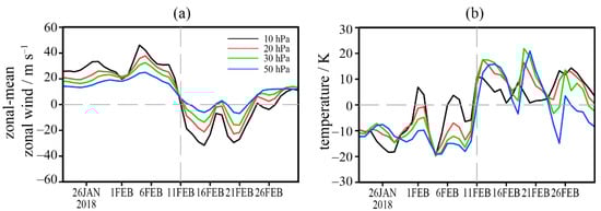
Figure 1.
Temporal evolutions of (a) the zonal-mean zonal wind averaged in 60–75° N and (b) meridional gradient of zonal-mean temperature between 60° N and the North Pole at 10–50 hPa during the period 22 January–3 March 2018 (within 40 days before and after the onset date of stratospheric sudden warming (SSW) shown by the vertical dashed line).
Figure 2 shows the temporal evolutions of the zonal-mean zonal wind averaged in 60–75° N and the air temperature averaged in the polar region (0–360°, 70–90° N) with their anomalies and tendency. Accompanying the reversal of zonal wind direction, positive (negative) anomalies of the zonal-mean zonal wind and negative (positive) anomalies of the air temperature are found in the polar region, indicating a relatively strong (weak) polar night jet and polar vortex before (after) the central date of the SSW (Figure 2a,b). The weakening of the zonal wind and the increase of the polar temperature mainly occurs during February 3–13 (Figure 2c,d). The maximum tendency of zonal wind and polar temperature appears around the central date. Fluctuations of the polar temperature tendency also exist after the occurrence of the SSW, but the center locates at relatively lower levels and with medium magnitudes (Figure 2d).
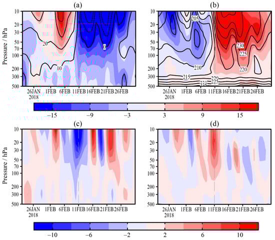
Figure 2.
Temporal evolutions of (a) the zonal-mean zonal wind (contour, unit: m s−1) with its anomaly (shading, unit: m s−1) and (c) tendency (unit: m s−1 d−1) averaged in 60–75° N during the period 22 January–3 March 2018. (b,d) As in (a,c), but for (b) the air temperature (contour, unit: K) with its anomaly (shading, unit: K) and (d) tendency (shading, unit: K d−1) averaged in the polar region (0–360°, 70–90° N).
The latitude–time cross sections of the zonal-mean zonal wind at 50–10 hPa is further given in Figure 3 to examine the possible influence of the SSW on the stratospheric mid-latitude circulation. During the period from late January to February, the QBO in the stratospheric tropical region displays the easterly phase, which favors the occurrence of the SSW event [11]. At 10 hPa, the polar easterly wind stretches widely in the meridional direction after the occurrence of the SSW, extending to 60° N on the central warming date. Five days later, the southernmost end of the easterly wind extends southward to 30° N (Figure 3a), but this phenomenon is not obvious at the lower levels. At 30–50 hPa, the reversal of the wind direction is limited to the north of 60° N (Figure 3c,d).
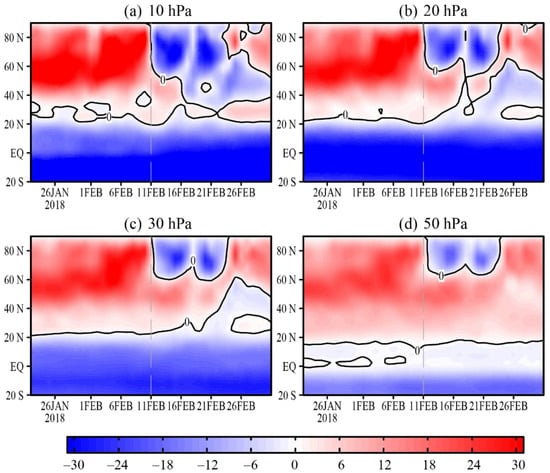
Figure 3.
The latitude–time cross sections of the zonal-mean zonal wind (unit: m s−1) during the period 22 January–3 March 2018 at (a) 10 hPa, (b) 20 hPa, (c) 30 hPa, and (d) 50 hPa, respectively.
Figure 4 illustrates distributions of the 5-day averaged geopotential height anomalies and the corresponding climatological planetary wavenumber-1 and wavenumber-2 components at 10 hPa during the period from 27 January to 15 February (15 days before and 5 days after the SSW). From 15 days to 10 days before the central date (Figure 4a), the geopotential height anomaly exhibits a zonal wavenumber-1 pattern. The negative anomaly center is located over the North Atlantic–European region, whereas the positive anomaly center is located over the Bering Strait, which is in phase with the climatological component of wavenumber 1. Five days before the SSW occurrence (Figure 4c), the positive geopotential height anomaly intrudes into the polar region from eastern Russia, North Atlantic and Northern Europe, and the negative geopotential height anomaly divides into two parts. The anomaly field of geopotential height shows a remarkable zonal wavenumber-2 pattern which is closely in phase with the climatological wavenumber 2. The polar vortex intensity is obviously weaker during this period. After the SSW occurrence, a strong positive anomaly dominates the polar region. The negative height anomalies mainly locate over the Northeastern Pacific and North America (Figure 4d).
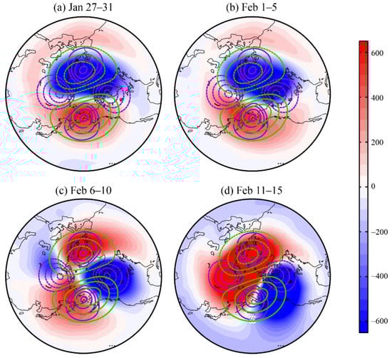
Figure 4.
10-hPa geopotential height anomalies averaged over each successive 5 days from 27 January to 15 February (shading, unit: gpm). Light green (purple) contours are the corresponding climatological wavenumber-1 (wavenumber-2) components. The contour levels for wavenumber 1 (wavenumber 2) are successively ± 200, ± 400, and ± 600 gpm (± 60, ± 90, ± 120, ± 150 gpm).
3.2. Dynamic Characteristics during the SSW Occurrence
3.2.1. Characteristics of Stratospheric Wave Activity
The occurrence of SSW event is caused by the interaction of planetary wave activity and the stratospheric mean flow. According to the dominant planetary wavenumbers (wavenumber 1 or 2) that lead to the breakdown of the stratospheric polar vortex, SSW events can be classified into wavenumber-1 and wavenumber-2 types. Charlton and Polvani [3] pointed out that the vortex displacement type and the vortex split type have a good correspondence with planetary wavenumber 1 and wavenumber 2 in the stratosphere, respectively. The following discussion will focus on the characteristics of planetary wave activities during the occurrence of February 2018 SSW. Figure 5 displays temporal evolutions of the vertical component of Eliassen–Palm (EPz) flux anomalies and EP flux divergence anomalies by planetary wavenumbers 1–3 averaged in 55–75° N at 10 hPa and 50 hPa, respectively. It is seen that a burst of wavenumber-1 EP flux appears during the period from 26 January to 1 February. A moderate magnitude of wavenumber-1 EP flux convergence is also found from 29 January to 2 February. This weakens the stratospheric polar vortex to a certain extent causing a minor warming event at 10 hPa (Figure 1 and Figure 5a,c). However, five days before the SSW occurrence, the 10-hPa wavenumber-2 EPz flux increases dramatically, accompanied by a negative anomaly of the wavenumber-1 component. The wavenumber-2 anomaly peaks around the central warming date (Figure 5a). Meanwhile, we see the maximum value of the convergence of wavenumber-2 EP flux on the central date (Figure 5c), implying the occurrence of a wavenumber-2 dominated SSW event.
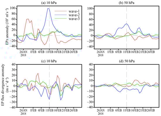
Figure 5.
Temporal evolutions of (a,b) the vertical component of Eliassen–Palm (EP) flux anomalies and (c,d) the divergence anomalies of EP flux in 55–75° N at (a,c) 10 hPa and (b,d) 50 hPa, respectively by planetary wavenumber 1 (red), 2 (blue) and 3 (green).
Barriopedro and Calvo [8] classified the SSW event into the wavenumber-2 type if, within 10 days before the SSW central date, the amplitude of the wavenumber-2 component of 10-day averaged geopotential height at 50 hPa along 60° N is greater than that of the wavenumber-1 component; or, the geopotential height amplitude of wavenumber 2 is greater than that of wavenumber 1, and their difference exceeds 200 gpm for more than 1 day. To see the dominant wavenumbers of planetary waves before the SSW, we also calculated the corresponding statistics following the above method and found that the February 2018 SSW is in full compliance with the definition of wavenumber-2 type in Barriopedro and Calvo [8] (Figure 6a). Therefore, although the sudden increase of wavenumber-1 EPz is observed 15–10 days before the SSW, overall, this SSW event is a polar vortex splitting event resulting from an anomalous increase of planetary wavenumber 2.
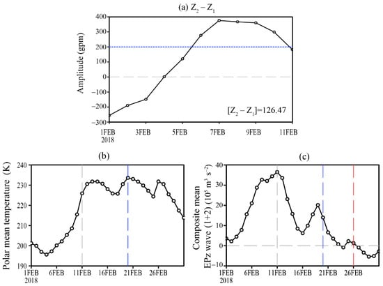
Figure 6.
Temporal evolutions of (a) the difference of geopotential height at 50 hPa along 60° N between wavenumber-1 and wavenumber-2 component, (b) the temperature averaged in the polar region (0–360°, 70–90° N) at 50 hPa, and (c) composite means of the EPz flux associated with wavenumber 1 and wavenumber 2 in 45–75° N at 100 hPa. Blue dashed line in (a) marks the 200 gpm. Gray dashed lines in (b,c) represent the onset date of the 2018 SSW event. Blue and red dashed lines represent the date when the maximum temperature in the polar region appears and the sixth day after it, respectively.
After the central date of the SSW, the wavenumber-2 EPz anomalies drop rapidly, whereas the wavenumber 1 displays negative anomaly for most of the time. After 16 February, the wavenumber-2 EPz anomaly increases again, which is more distinguished at 50 hPa (Figure 5b). And the wavenumber-3 EPz is also observed with relatively large positive anomaly. The intensive convergence reappears in the EP flux of wavenumber 2 and wavenumber 3 at 10 hPa, which matches the reappearance of warming in the stratospheric polar region and the decrease of the zonal easterly wind one week after the SSW (Figure 1).
Kodera et al. [9] discussed the wave activity characteristics after the SSW occurrence. They classified SSW events into two different types based on the propagation direction of the planetary wave after the central date—the absorbing type and the reflecting type. According to the classification, a key date (Dtmax) is defined when the polar temperature at 50 hPa reaches the maximum. On the Dtmax or during its following 6 days, if the composite mean of the wavenumber-1 and wavenumber-2 EPz averaged in 45–75° N at 100 hPa is negative for more than two days, this event is identified as a SSW event of reflecting type, otherwise it is considered as a SSW event of absorbing type. Figure 6b,c shows the temporal evolutions of the temperature averaged in the polar region (0–360°, 70–90° N) at 50 hPa and the composite means of wavenumber-1 and wavenumber-2 EPz flux in 45–75° N at 100 hPa. We see that the highest polar temperature does not occur on the central date. After the SSW, the polar temperature continues to rise. Although the temperature drops somewhat during this period, the highest polar temperature appears on 20 February (Figure 6b). Within the following 6 days, there is only one day when the composite mean of the wavenumber-1 and wavenumber-2 EPz flux is negative (Figure 6c). Therefore, the February 2018 SSW event can be classified as an absorbing type.
3.2.2. Tropospheric Precursory Signals before the SSW
It was generally believed that the planetary wave in the extratropical stratosphere originates from the troposphere. However, recent studies found that an enhanced wave activity in the troposphere is not necessarily responsible for the SSW occurrence. Only 30–35% SSWs is preceded by extreme tropospheric wave activity [28,29,30]. To examine whether the 2018 SSW event is preceded by an active tropospheric wave activity, Figure 7 shows the temporal evolutions of standardized EPz flux in 45–75° N associated with wavenumber 1 and wavenumber 2. Following the method in Birner and Albers [29], the standardized EPz flux is calculated by normalized by its daily standard deviations during 1979–2018.
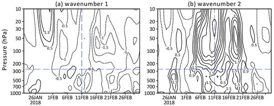
Figure 7.
Temporal evolutions of standardized EPz flux in 45–75° N associated with (a) wavenumber 1 and (b) wavenumber 2. Contour interval is 0.5 with zero lines omitted. Vertical dashed lines represent the onset date of 2018 SSW event. Horizontal dashed lines represent the approximate tropopause level.
Consistent with Figure 5a, positive anomalies of wavenumber 1 are mainly confined in the stratosphere from 26 January to 1 February. Positive wavenumber-1 EPz flux is also observed in the troposphere in the days around 26 January. However, there is no apparent linkage between the wavenumber-1 EPz flux in the stratosphere and troposphere (Figure 7a). In contrast, the magnitude of standardized EPz flux by wavenumber 2 is much larger than that of wavenumber 1, especially from 5 days before to 10 days following the SSW onset (Figure 7b). In the mid-troposphere, we see a moderate magnitude (~1.5 standard deviations) of wavenumber-2 flux five days prior to the SSW onset date. Furthermore, the wavenumber-2 flux in the troposphere is closely connected to that in the stratosphere, which indicates that the 2018 SSW event is preceded by an active tropospheric wavenumber-2 activity.
Garfinkel et al. [31] believed that the in-phase superposition of the local positive (negative) anomalies of the geopotential height and the ridge (trough) of the climatological stationary wave can enhance the upward propagation of tropospheric planetary waves, whereas the out-phase superposition can weaken the upward propagation. To further examine the tropospheric precursory signals, Figure 8 illustrates the 500-hPa geopotential height anomalies averaged over 10 days (1–10 February) before the SSW occurrence and the zonal deviations of climatological geopotential height in the corresponding period. It is obvious that within 10 days before the SSW, the negative anomaly center of geopotential height is mainly located over the northeastern North America and the Greenland. There are three positive anomaly centers locating over Central Siberia, North Atlantic, as well as Alaska and Northeast Pacific south of it, respectively. At this moment, the trough of climatological stationary waves in the Northern Hemisphere is located above East Asia, Northwest Pacific and the northeastern North America. The ridge is mainly located over Alaska, the western North America, North Atlantic and the Eastern Europe. The climatological trough over the northeastern North America and the Alaska ridge are obviously in phase with the geopotential height anomalies located at these corresponding areas before the SSW. It greatly facilitates the development and propagation of the tropospheric planetary wave into the stratosphere. The tropospheric distribution of geopotential height anomalies before the SSW in winter of 2018 is quite similar to that of the wavenumber-2 SSW event in January of 2009 [19,32].
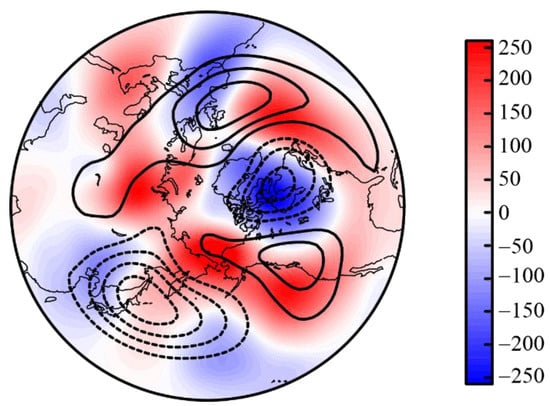
Figure 8.
The distribution of geopotential height anomalies at 500 hPa averaged over 10 days (1–10 February) before the SSW onset (shading, unit: gpm). Contours are the zonal deviations of climatological geopotential height in the corresponding period (interval: 50 gpm, zero lines are omitted).
To further understand the influence of the precursory signals in the tropospheric key areas on the stratospheric planetary waves, we perform the harmonic analysis of the 10-day averaged geopotential height anomaly before the SSW. Figure 9 shows the anomalies of wavenumber-1 and wavenumber-2 component at 500 hPa and 10 hPa. It is seen that at 500 hPa, the wavenumber-1 height anomalies have a large phase difference with the climatology (Figure 9a), which contributes little to the development of planetary wavenumber 1 in the mid-troposphere. Meanwhile, at 10 hPa, the wavenumber-1 height anomalies are almost orthogonal to the climatology, indicating a dormant planetary wavenumber-1 activity in the stratosphere (Figure 9c). However, at 500 hPa, the anomaly of tropospheric planetary wavenumber 2 is obviously in phase with the climatological component (Figure 9b), which greatly enhances the propagation of planetary wavenumber 2 from the extratropical troposphere to stratosphere. At 10 hPa, the highly in-phase relationship between the wavenumber-2 height anomaly and the climatological component is also observed (Figure 9d), which proves once again that this SSW event is a polar vortex splitting event dominated by planetary wavenumber 2.
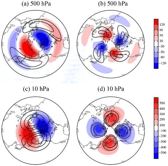
Figure 9.
The (a,c) wavenumber-1 and (b,d) wavenumber-2 components of geopotential height anomalies (shadeding, unit: gpm) at (a,b) 500 hPa and (c,d) 10 hPa averaged over 10 days (1–10 February) before the 2018 SSW onset. Contours are climatological wavenumber-1 and wavenumber-2 components in the corresponding period. The contour levels are successively ± 200, ± 400, and ± 600 gpm in (c) and ± 60, ± 90 gpm in (a,b,d), respectively.
3.3. Near-Surface Temperature Response after the SSW
In this section, the possible impacts of the February 2018 SSW event on surface weather over the North America are discussed. Figure 10 shows the 5-day averaged 2-meter temperature anomalies within 30 days before and after the central SSW date. It can be seen that after the SSW, the North America experiences a cold wave. From 1 to 5 days after the SSW (days 1–5), the main cooling area is confined in the northeastern Canada. There are only scattered low temperature centers in the western North America (Figure 10d). On days 6–10, the low temperature area in the western North America and northeastern Canada has developed to a great extent (Figure 10e). The large areas of low temperature disappear in Canada by days 11–15, and the low temperature areas in the western North America is mainly located in the western United States (Figure 10f). Such a cold wave process suggests that the 2018 SSW may have an important impact on the weather in North America. However, by comparing Figure 10b,c with Figure 10d,e, we note that the cold extremes in the northern part of North America have occurred 10 days before the SSW.
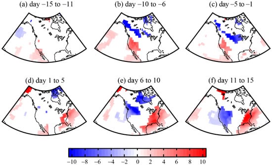
Figure 10.
The 2-meter temperature anomalies (unit: K) averaged over each successive 5 days within 30 days before and after the onset date of 2018 SSW event. Shadings represent the anomalies that exceed the 0.8 standard deviations of the 2-meter temperature in February during the period 1979–2018.
To examine the corresponding circulation pattern in the mid-troposphere during the life cycle of 2018 SSW, Figure 11a shows the longitude–time evolution of the zonal deviation of the 500-hPa geopotential height averaged in 60–70° N before and after the SSW. It is seen that a distinct structure, namely high-pressure anomaly in Alaska region (approximately over 170–135°W) and low-pressure anomaly in northeastern North America (105–50°W), persists in the days before and after the 2018 SSW event. The centers exceeding 300 gpm first appear in late January and early February for the high and low pressure, respectively. This tropospheric circulation pattern, or such a west–east dipole, has two effects. First, it favors the increase of tropospheric wavenumber 2 flux and propagation to the extratropical stratosphere, leading to the occurrence of 2018 SSW event. Moreover, it is conducive to the cold air moving southward from the polar region along the northerly wind between the east side of the high pressure and the west side of the low pressure, causing cold extremes in North America (Figure 10b–e).
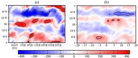
Figure 11.
(a) The longitude–time cross section of the zonal deviation of geopotential height in 60–70° N at 500 hPa within 40 days before and after the onset date of SSW in the winter of 2018. (b) As in (a), but for the composite constructed with respect of the onset dates of the other seven SSW cases. The vertical dashed lines represent the SSW onset dates. The contour levels are 300 and 200 gpm in (a) and (b), respectively.
Although the effect of above west–east dipole on the weather over North America is understandable, it is noted that the 2018 SSW’s role could not be ruled out. We speculate that SSW may interact with the dipole, especially the high pressure in Alaska, resulting in the cold waves. In fact, several previous studies suggest the relationship between the SSW and the occurrence of tropospheric blocking high may be interacting. On the one hand, the occurrence of blocking high could stimulate the upward propagation of planetary wave and leads to the breakdown of the stratospheric polar vortex and SSWs. On the other hand, after the SSW onset, the disturbed stratospheric flow may have a positive feedback to the maintenance of blocking high [13,33]. Kodera et al. [34,35] pointed out that the stratospheric flow after the SSWs traps the planetary waves and thus leads to amplification of tropospheric planetary waves, which in turn produces a favorable condition for blocking occurrence around an enhanced ridge of planetary waves, in particular over the North Pacific sector.
To further confirm the speculation, we revisit the major SSW events in the NCEP–NCAR reanalysis data during the relatively short period 1979–2017. After the onset date, in total seven out of 23 major SSWs feature with the similar mid-tropospheric dipole to the 2018 event. The central dates of the above seven SSWs are 22 February 1979, 26 February 1984, 20 February 1989, 17 December 1998, 11 February 2001, 4 January 2004, and 7 January 2013, respectively. We show the tropospheric circulation pattern in Figure 11b composited by the seven SSWs with respect to the onset dates. As expected after the SSW, an anomalous high-pressure ridge is observed in the mid-troposphere over Alaska and an anomalous low-pressure trough exists in the northeastern North America. This west–east dipole lasts for 15–20 days. Figure 12 shows the composite 2-meter temperature anomalies associated with the seven SSWs. While there is almost no significantly anomalous signals in North American continent within 15 days before the SSW (Figure 12a–c), significantly negative temperature anomalies appear and expand with time in the Northeastern and Central Canada with the emergence of the pronounced mid-tropospheric dipole after the SSW onset (Figure 12d–f). The cold anomalies can last up to 20 days (Figures not shown). It is not difficult to find from the above analyses that cold waves are likely to happen following this type of SSW onset. Although we cannot conclude in this kind of study that it is the SSWs that exert profound impacts on the surface weather over North America, to some extent such coincidence increases the reasonability that the 2018 SSW event could affect the weather in North America through the mid-tropospheric dipole.
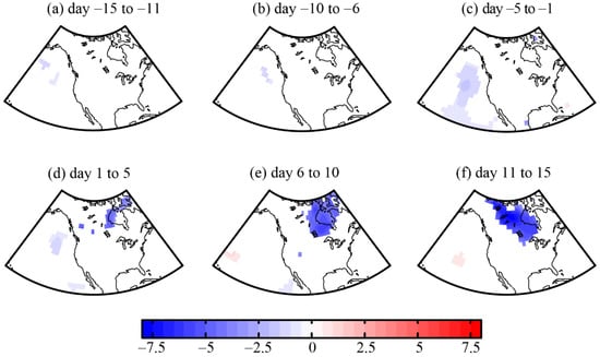
Figure 12.
As in Figure 10, but for the composite of other 7 SSW events. Shadings represent the anomalies significantly different from zero at 95% confidence level based on the two tailed Student’s t-test.
4. Conclusions
In this paper, NCEP–NCAR daily reanalysis data is used to analyze the evolution of the extratropical stratospheric circulation and the dynamic characteristics during the occurrence of the SSW event in the winter of 2018. The types of this SSW event are identified and the tropospheric precursory signals for this SSW event are examined. Finally, the possible impacts of the SSW on the weather over North America are investigated. The main conclusions are as follows.
Following the definition given by WMO, this SSW event is classified into major warming event. The central date is 11 February 2018. About one week before the SSW, the polar temperature in the middle and lower stratosphere increases and the polar night jet weakens. The tendency of the zonal-mean zonal wind and the polar temperature reach the maximum around the central date. After the SSW, the 10-hPa stratosphere exhibits a close linkage between the circulation in polar region and that at the middle latitudes, which gradually weakens with the decreasing height.
The dynamic diagnosis reveals that the wavenumber-1 EPz anomaly increases abruptly from 15 to 10 days before the SSW, resulting in a minor warming at 10 hPa and the weakening of the stratospheric polar vortex. However, the wavenumber-2 EPz anomaly increases drastically about one week before the SSW. Meanwhile, the EP flux of wavenumber-2 component converges strongly in the high-latitude stratosphere and peaks on the central date of the SSW. At this moment, two pairs of positive and negative anomaly centers appear in the stratospheric polar region, indicating a polar vortex splitting SSW event dominated by planetary wavenumber 2. Moreover, the composite mean of EPz of wavenumber-1 and wavenumber-2 component at 100 hPa is negative for only 1 day out of 7 days since the polar temperature reaches its maximum, denoting that the event is also a SSW event of absorbing type. However, the 2018 SSW might not be a purely splitting event. As seen in Figure 4, the stratospheric polar vortex evolves from a displacement to a splitting type, finally back to the displacement type disturbance. This complex behavior is typical, which is consistent with the evolutions of stratospheric polar vortex in most SSWs [36].
The main precursory signals before the SSW event include the ridge over Alaska and the trough over the northeastern North America in the mid-troposphere. The distributions of the trough and ridge exhibit a general in-phase relationship with that of the climatological planetary wavenumber 2 in the troposphere, which greatly enhance the propagation of planetary wavenumber 2 towards the extratropical stratosphere. These signals appear within 15–10 days before the SSW and last for about 10 days after the central date, implying that there may be an interaction between the 2018 SSW event and the tropospheric blocking high.
The 2018 SSW event may exert a remarkable influence on the weather over North America via the SSW-related west–east dipole, namely a ridge over Alaska and a trough over the northeastern North America in the mid-troposphere that lasted up to 10 days after the onset date. Composite analysis of the other seven SSW events to some extent verifies this finding although the sample size is relatively small. We suggest that the temperature in the northeastern and central Canada could be significantly reduced within 10 days after this type of SSW that favors an emergence of such a dipole over the North Pacific–North America region.
Author Contributions
Conceptualization, J.H.; formal analysis, J.X.; data curation, S.L. and H.H.; writing—original draft preparation, J.X. and J.H.; writing—review and editing, J.H., H.X., S.L., and H.H. All authors have read and agreed to the published version of the manuscript.
Funding
This work was jointly supported by the NSFC Project (41975048 and 41975106), Jiangsu NSF Project (BK20191404), and National Training Program of Innovation and Entrepreneurship for Undergraduates (201810300011Z).
Acknowledgments
The authors thank two anonymous reviewers and the editor for their helpful comments.
Conflicts of Interest
The authors declare no conflict of interest.
References
- Scherhag, R. Die Explosionsartigen Stratosphärenerwärmungen des Spätwinters 1951–1952. Ber. Dtsch. Wetterdienst 1952, 6, 51–63. [Google Scholar]
- Andrews, D.G.; Holton, J.R.; Leovy, C.B. Middle Atmosphere Dynamics; Academic Press: San Diego, CA, USA, 1987; p. 489. [Google Scholar]
- Charlton, A.J.; Polvani, L.M. A new look at stratospheric sudden warmings. Part I: Climatology and modeling benchmarks. J. Clim. 2007, 20, 449–469. [Google Scholar] [CrossRef]
- Kuttippurath, J.; Nikulin, G. A comparative study of the major sudden stratospheric warmings in the Arctic winters 2003/2004–2009/2010. Atmos. Chem. Phys. 2012, 12, 8115–8129. [Google Scholar] [CrossRef]
- WMO CAS. Abridged Final Report of the Seventh Session, Manila, 27 February–10 March 1978; Secretariat of the WMO Rep. WMO-509; WMO: Geneva, Switzerland, 1978; p. 113. [Google Scholar]
- Labitzke, K.; Naujokat, B. The lower arctic stratosphere in winter since 1952. SPARC Newsl. 2000, 15, 11–14. [Google Scholar]
- Bancala, S.; Kruger, K.; Giorgetta, M. The preconditioning of major sudden stratospheric warmings. J. Geophys. Res. 2012, 117, D04101. [Google Scholar] [CrossRef]
- Barriopedro, D.; Calvo, N. On the relationship between ENSO, stratospheric sudden warmings, and blocking. J. Clim. 2014, 27, 4704–4720. [Google Scholar] [CrossRef]
- Kodera, K.; Mukougawa, H.; Maury, P.; Ueda, M.; Claud, C. Absorbing and reflecting sudden stratospheric warming events and their relationship with tropospheric circulation. J. Geophys. Res. Atmos. 2016, 121, 80–94. [Google Scholar] [CrossRef]
- Matsuno, T. A dynamical model of the stratospheric sudden warming. J. Atmos. Sci. 1971, 28, 1479–1494. [Google Scholar] [CrossRef]
- Holton, J.R.; Tan, H.C. The influence of the equatorial Quasi-Biennial Oscillation on the global circulation at 50 mb. J. Atmos. Sci. 1980, 37, 2200–2208. [Google Scholar] [CrossRef]
- García-Herrera, R.; Calvo, N.; Garcia, R.; Giorgetta, M. Propagation of ENSO temperature signals into the middle atmosphere: A comparison of two general circulation models and ERA-40 reanalysis data. J. Geophys. Res. 2006, 111, D06101. [Google Scholar] [CrossRef]
- Martius, O.; Polvani, L.M.; Davies, H.C. Blocking precursors to stratospheric sudden warming events. Geophys. Res. Lett. 2009, 36, L14806. [Google Scholar] [CrossRef]
- Woollings, T.; Charlton-Perez, A.; Ineson, S.; Marshall, A.G.; Masato, G. Associations between stratospheric variability and tropospheric blocking. J. Geophys. Res. 2010, 115, D06108. [Google Scholar] [CrossRef]
- Hu, J.G.; Li, T.; Xu, H.M.; Yang, S.Y. Lessened response of boreal winter stratospheric polar vortex to El Niño in recent decades. Clim. Dyn. 2017, 49, 263–278. [Google Scholar] [CrossRef]
- Mitchell, D.M.; Gray, L.J.; Charlton-Perez, A.J. The structure and evolution of the stratospheric vortex in response to natural forcings. J. Geophys. Res. 2011, 116, D15110. [Google Scholar] [CrossRef]
- Limpasuvan, V.; Thompson, D.W.J.; Hartmann, D.L. The life cycle of the Northern Hemisphere sudden stratospheric warmings. J. Clim. 2004, 17, 2584–2596. [Google Scholar] [CrossRef]
- Kruger, K.; Naujokat, B.; Labitzke, K. The unusual midwinter warming in the Southern Hemisphere stratosphere 2002: A comparison to northern hemisphere phenomena. J. Atmos. Sci. 2005, 62, 603–613. [Google Scholar] [CrossRef]
- Harada, Y.; Goto, A.; Hasegawa, H.; Fujikawa, N.; Naoe, H.; Hirooka, T. A major stratospheric sudden warming event in January 2009. J. Atmos. Sci. 2010, 67, 2052–2069. [Google Scholar] [CrossRef]
- Ayarzagüena, B.; Langematz, U.; Serrano, E. Tropospheric forcing of the stratosphere: A comparative study of the two different major stratospheric warmings in 2009 and 2010. J. Geophys. Res. 2011, 116, D18114. [Google Scholar] [CrossRef]
- Manney, G.L.; Lawrence, Z.D.; Santee, M.L.; Read, W.G.; Livesey, N.J.; Lambert, A.; Froidevaux, L.; Pumphrey, H.C.; Schwartz, M.J. A minor sudden stratospheric warming with a major impact: Transport and polar processing in the 2014/2015 Arctic winter. Geophys. Res. Lett. 2015, 42, 7808–7816. [Google Scholar] [CrossRef]
- Shi, C.; Xu, T.; Guo, D.; Pan, Z. Modulating effects of planetary wave 3 on a stratospheric sudden warming event in 2005. J. Atmos. Sci. 2017, 74, 1549–1559. [Google Scholar] [CrossRef]
- Rao, J.; Ren, R.; Chen, H.; Yu, Y.; Zhou, Y. The stratospheric sudden warming event in February 2018 and its prediction by a climate system model. J. Geophys. Res. Atmos. 2018, 123, 13332–13345. [Google Scholar] [CrossRef]
- Rao, J.; Garfinkel, C.I.; White, I.P. Predicting the downward and surface influence of the February 2018 and January 2019 sudden stratospheric warming events in subseasonal to seasonal (S2S) models. J. Geophys. Res. Atmos. 2020, 125. [Google Scholar] [CrossRef]
- Wang, Y.; Shulga, V.; Milinevsky, G.; Patoka, A.; Evtushevsky, O.; Klekociuk, A.; Han, W.; Grytsai, A.; Shulga, D.; Myshenko, V.; et al. Winter 2018 major sudden stratospheric warming impact on midlatitude mesosphere from microwave radiometer measurements. Atmos. Chem. Phys. 2019, 19, 10303–10317. [Google Scholar] [CrossRef]
- Lü, Z.; Li, F.; Orsolini, Y.J.; Gao, Y.; He, S. Understanding of european cold extremes, sudden stratospheric warming, and siberian snow accumulation in the winter of 2017/18. J. Clim. 2020, 33, 527–545. [Google Scholar] [CrossRef]
- Kalnay, E.; Kanamitsu, M.; Kistler, R.; Collins, W.; Deaven, D.; Gandin, L.; Iredell, M.; Saha, S.; White, G.; Woollen, J.; et al. The NCEP/NCAR 40-year reanalysis project. Bull. Am. Meteorol. Soc. 1996, 77, 437–471. [Google Scholar] [CrossRef]
- Jucker, M. Are sudden stratospheric warmings generic? Insights from an Idealized GCM. J. Atmos. Sci. 2016, 73, 5061–5080. [Google Scholar] [CrossRef]
- Birner, T.; Albers, J.R. Sudden stratospheric warmings and anomalous upward wave activity flux. SOLA 2017, 13A, 8–12. [Google Scholar] [CrossRef]
- de la Cámara, A.; Birner, T.; Albers, J.R. Are sudden stratospheric warmings preceded by anomalous tropospheric wave activity? J. Clim. 2019, 32, 7173–7189. [Google Scholar] [CrossRef]
- Garfinkel, C.I.; Hartmann, D.L.; Sassi, F. Tropospheric precursors of anomalous Northern Hemisphere stratospheric polar vortices. J. Clim. 2010, 23, 3282–3299. [Google Scholar] [CrossRef]
- Li, Y.F.; Hu, J.G.; Ren, R.C. A case study of the Northern Hemisphere sudden warming in the winter of 2009. Plateau Meteor. 2017, 36, 1576–1586, (In Chinese with English abstract). [Google Scholar]
- Woollings, T.; Hoskins, B. Simultaneous Atlantic-Pacific blocking and the Northern Annular Mode. Q. J. Roy. Meteor. Soc. 2008, 134, 1635–1646. [Google Scholar] [CrossRef]
- Kodera, K.; Mukougawa, H.; Itoh, S. Tropospheric impact of reflected planetary waves from the stratosphere. Geophys. Res. Lett. 2008, 35, L16806. [Google Scholar] [CrossRef]
- Kodera, K.; Mukougawa, H.; Fujii, A. Influence of the vertical and zonal propagation of stratospheric planetary waves on tropospheric blockings. J. Geophys. Res. Atmos. 2013, 118, 8333–8345. [Google Scholar] [CrossRef]
- Ehrmann, T.S.; Colucci, S.J. A thermodynamic climatology of the disturbed stratospheric polar vortex. Int. J. Climatol. 2019, 39, 3241–3256. [Google Scholar] [CrossRef]
© 2020 by the authors. Licensee MDPI, Basel, Switzerland. This article is an open access article distributed under the terms and conditions of the Creative Commons Attribution (CC BY) license (http://creativecommons.org/licenses/by/4.0/).