Spatio-Temporal Trends of Monthly and Annual Precipitation in Aguascalientes, Mexico


 ,
,  and
and
Abstract
1. Introduction
2. Materials and Methods
2.1. Area of Study
2.2. Meteorological Data
2.3. Statistical Analysis
3. Results and Discussion
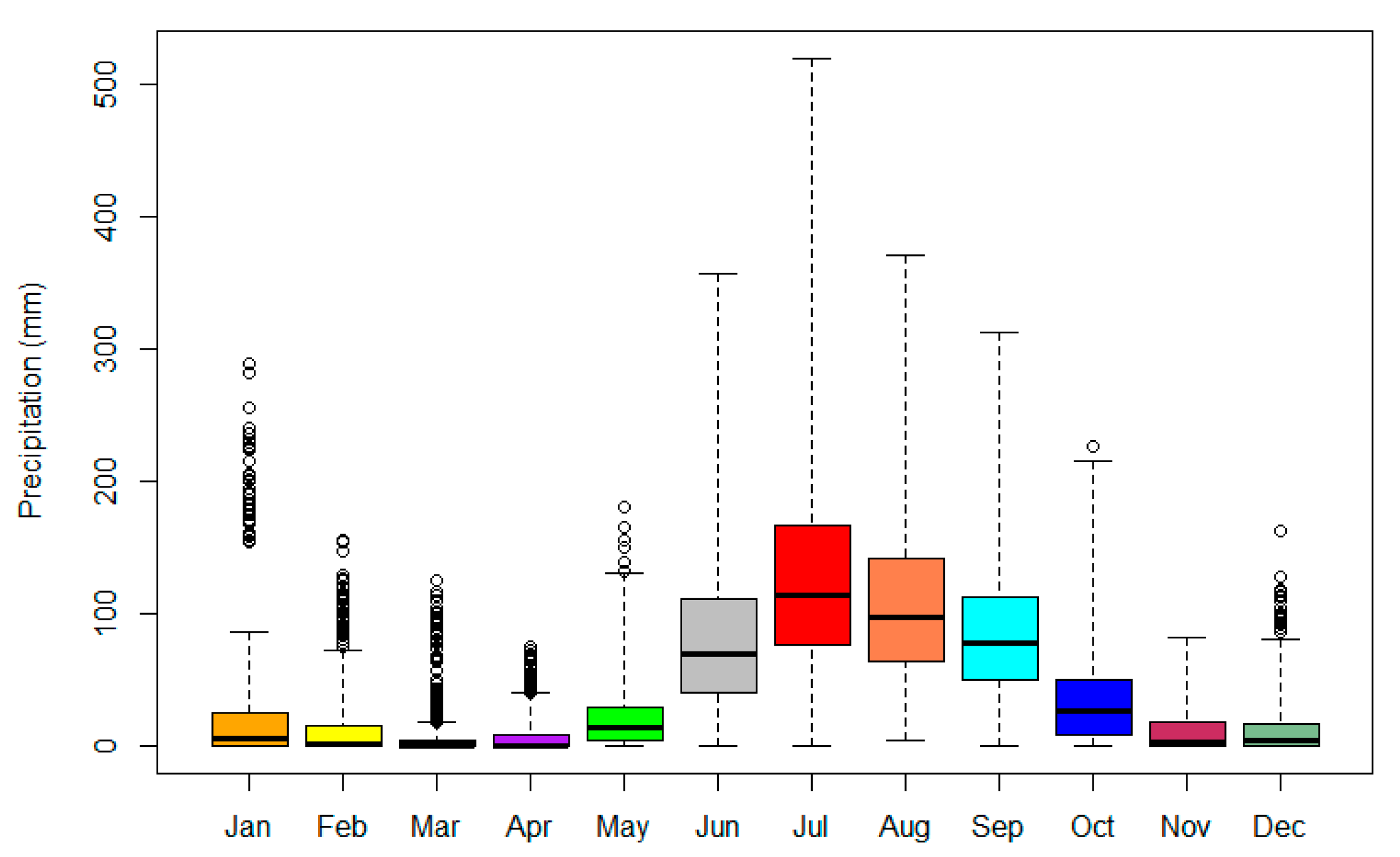
3.1. Distribution of Data
3.2. Observed Trends
3.2.1. Monthly Trends
Statistically Significant Negative Trends
Statistically Significant Positive Trends
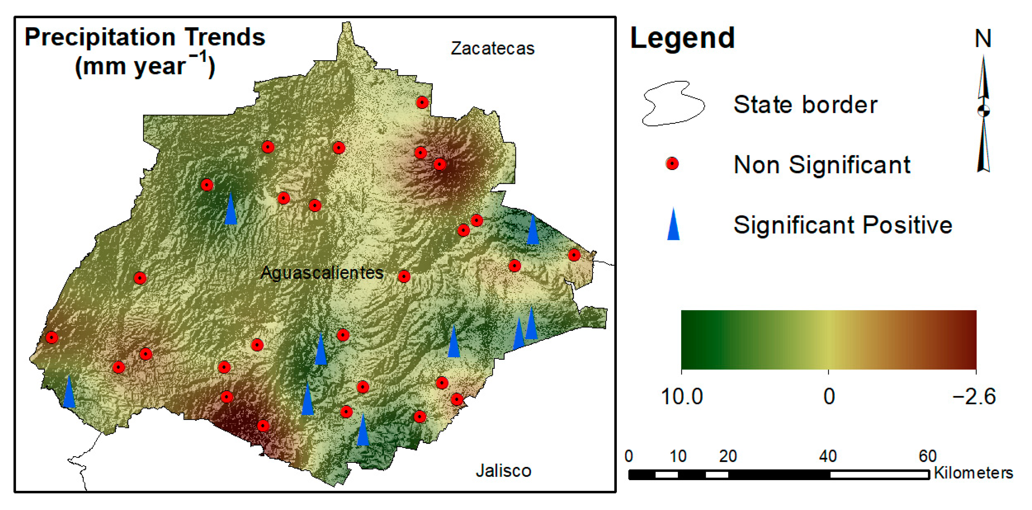
3.2.2. Annual Trend
3.3. Possible Causes of Statistically Significant Negative Trends
3.4. Possible Causes of Statistically Significant Positive Trends
3.5. Other Possible Factors Responsible for Precipitation Changes in Aguascalientes
4. Conclusions
Author Contributions
Funding
Acknowledgments
Conflicts of Interest
References
- Wuebbles, D.J.; Fahey, D.W.; Hibbard, K.A.; DeAngelo, B.; Doherty, S.; Hayhoe, K.; Horton, R.; Kossin, J.P.; Taylor, P.C.; Waple, A.M.; et al. Climate Science Special Report: Fourth National Climate Assessment, Volume I; Wuebbles, D.J., Fahey, D.W., Hibbard, K.A., Dokken, D.J., Stewart, B.C., Maycock, T.K., Eds.; U.S. Global Change Research Program: Washington, DC, USA, 2017; pp. 12–34. [CrossRef]
- World Meteorological Organization (WMO). Available online: http://www.wmo.int/pages/prog/wcp/ccl/faq/faq_doc_en.html (accessed on 15 January 2020).
- IPCC. IPCC. Climate Change 2013: The Physical Science Basis; Contribution of Working Group I to the Fifth Assessment Report of the Intergovernmental Panel on Climate Change; Stocker, T.F., Qin, D., Plattner, G.K., Tignor, M., Allen, S.K., Boschung, J., Nauels, A., Xia, Y., Bex, C., Midgley, P.M., Eds.; Cambridge University Press: Cambridge, UK, 2013; p. 1535. [Google Scholar]
- IPCC. IPCC. Climate Change 2001: The Scientific Basis; Contribution of Working Group I to the Third Assessment Report of the Intergovernmental Panel on Climate Change; Houghton, J.T., Ding, Y., Griggs, D.J., Noguer, M., van der Linden, P.J., Dai, X., Maskell, K., Johnson, C.A., Eds.; Cambridge University Press: Cambridge, UK, 2001. [Google Scholar]
- Rakhecha, P.R.; Singh, V.P. Applied Hydrometeorology; Springer: New York, NY, USA, 2009; 384p. [Google Scholar]
- Rodriguez-Puebla, C.; Encinas, A.H.; Nieto, S.; Garmendia, J. Spatial and temporal patterns of annual precipitation variability over The Iberian Peninsula. Int. J. Climatol. 1998, 18, 299–316. [Google Scholar] [CrossRef]
- Chattopadhyay, S.; Edwards, D.R. Long-Term Trend Analysis of Precipitation and Air Temperature for Kentucky, United States. Climate 2016, 4, 10. [Google Scholar] [CrossRef]
- Asakereh, H. Trends in monthly precipitation over the northwest of Iran (NWI). Theor. Appl. Climatol. 2017, 130, 443–451. [Google Scholar] [CrossRef]
- Zhang, Q.; Xu, C.Y.; Zhang, Z.; Chen, Y.D.; Liu, C.; Lin, H. Spatial and temporal variability of precipitation maxima during 1960-2005 in the Yangtze River basin and possible association with large-scale circulation. J. Hydrol. 2008, 353, 215–227. [Google Scholar] [CrossRef]
- Menzel, L.; Burger, G. Climate change scenarios and runoff response in the Mulde catchment (Southern Elbe, Germany). J. Hydrol. 2002, 267, 53–64. [Google Scholar] [CrossRef]
- Brown, K.; Kamruzzaman, M.; Beecham, S. Trends in sub-daily precipitation in Tasmania using regional dynamically downscaled climate projections. J. Hydrol. Reg. Stud. 2017, 10, 18–34. [Google Scholar] [CrossRef]
- Beharry, S.L.; Clarke, R.M.; Kurmarsingh, K. Precipitation trends using in-situ and gridded datasets. Theor. Appl. Climatol. 2014, 115, 599–607. [Google Scholar] [CrossRef]
- Młyński, D.; Cebulska, M.; Wałęga, A. Trends, Variability, and Seasonality of Maximum Annual Daily Precipitation in the Upper Vistula Basin, Poland. Atmosphere 2018, 9, 313. [Google Scholar] [CrossRef]
- Gemmer, M.; Becker, S.; Jiang, T. Observed monthly precipitation trends in China 1951–2002. Theor. Appl. Climatol. 2004, 77, 39–45. [Google Scholar] [CrossRef]
- Gedefaw, M.; Yan, D.; Wang, H.; Qin, T.; Girma, A.; Abiyu, A.; Batsuren, D. Innovative Trend Analysis of Annual and Seasonal Rainfall Variability in Amhara Regional State, Ethiopia. Atmosphere 2018, 9, 326. [Google Scholar] [CrossRef]
- Bougara, H.; Hamed, K.B.; Borgemeister, C.; Tischbein, B.; Kumar, N. Analyzing Trend and Variability of Rainfall in The Tafna Basin (Northwestern Algeria). Atmosphere 2020, 11, 347. [Google Scholar] [CrossRef]
- Khaniya, B.; Jayanayaka, I.; Jayasanka, P.; Rathnayake, U. Rainfall Trend Analysis in Uma Oya Basin, Sri Lanka, and Future Water Scarcity Problems in Perspective of Climate Variability. Adv. Meteorol. 2019, 2019, 3636158. [Google Scholar] [CrossRef]
- Partal, T.; Kahya, E. Trend analysis in Turkish precipitation data. Hydrol. Process. 2006, 20, 2011–2026. [Google Scholar] [CrossRef]
- Sayemuzzaman, M.; Jha, M.K. Seasonal and annual precipitation time series trend analysis in North Carolina, United States. Atmos. Res. 2014, 137, 183–194. [Google Scholar] [CrossRef]
- Tabari, H.; Talaee, P.H. Temporal variability of precipitation over Iran: 1966–2005. J. Hydrol. 2011, 396, 313–320. [Google Scholar] [CrossRef]
- Zhao, W.; Yu, X.; Ma, H.; Zhu, Q.; Zhang, Y.; Qin, W.; Ai, N.; Wang, Y. Analysis of Precipitation Characteristics during 1957–2012 in the Semi-Arid Loess Plateau, China. PLoS ONE 2015, 10, e0141662. [Google Scholar] [CrossRef]
- Caloiero, T.; Coscarelli, R.; Ferrari, E. Analysis of Monthly Rainfall Trend in Calabria (Southern Italy) through the Application of Statistical and Graphical Techniques. Proceedings 2018, 2, 629. [Google Scholar] [CrossRef]
- Gebrechorkos, S.H.; Hulsmann, S.; Bernhofer, C. Long-term trends in rainfall and temperature using high-resolution climate datasets in East Africa. Nature 2019, 9, 11376. [Google Scholar] [CrossRef] [PubMed]
- Gentilucci, M.; Barbieri, M.; Lee, H.S.; Zardi, D. Analysis of Rainfall Trends and Extreme Precipitation in the Middle Adriatic Side, Marche Region (Central Italy). Water 2019, 11, 1948. [Google Scholar] [CrossRef]
- Gonzalez-Hidalgo, J.C.; Lopez-Bustins, J.A.; Stepanek, P.; Martin-Vide, J.; de Luis, M. Monthly precipitation trends on the Mediterranean fringe of the Iberian Peninsula during the second-half of the twentieth century (1951–2000). Int. J. Climatol. 2009, 29, 1415–1429. [Google Scholar] [CrossRef]
- Jones, P.D.; Harpham, C.; Harris, I.; Goodess, C.M.; Burton, A.; Centella-Artola, A.; Taylor, M.A.; Bezanilla-Morlot, A.; Campbell, J.D.; Stephenson, T.N.; et al. Long-term trends in precipitation and temperature across the Caribbean. Int. J. Climatol. 2016, 36, 3314–3333. [Google Scholar] [CrossRef]
- Cavazos, T.; Hastenrath, S. Convection and rainfall over Mexico and their modulation by the southern oscillation. Int. J. Climatol. 1990, 10, 377–386. [Google Scholar] [CrossRef]
- Arriaga-Ramirez, S.; Cavazos, T. Regional trends of daily precipitation indices in Northwest Mexico and Southwest United States. J. Geophys. Res. 2010, 115, D14. [Google Scholar] [CrossRef]
- Karmalkar, A.V.; Bradley, R.S.; Diaz, H.F. Climate change in Central America and Mexico: Regional climate model validation and climate change projections. Clim. Dyn. 2011, 37, 605–629. [Google Scholar] [CrossRef]
- Ochoa, C.A.; Quintanar, A.I.; Raga, G.B. Changes in intense precipitation events in Mexico City. J. Hydrometeorol. 2015, 16, 1804–1820. [Google Scholar] [CrossRef]
- Instituto Nacional de Investigaciones Forestales Agricolas y Pecuarias (INIFAP). Agenda Técnica Agrícola de Aguascalientes; Delegacion Coyoacan: Ciudad de Mexico, Mexico, 2017; 132p. [Google Scholar]
- Lemus, L.; Gay, C. Temperature, precipitation variations and focal effects Aguascalientes 1921–1985. Atmósfera 2009, 39–44. [Google Scholar]
- Ruíz Álvarez, O.; Espejel Trujano, D.; Ontiveros Capurata, R.E.; Enciso, J.M.; Galindo Reyes, M.A.; Quesada Parga, M.L.; Grageda Grageda, J.; Ramos Reyes, R.; Ruíz Corral, J.A. Tendencia de temperaturas máximas y mínimas mensuales en Aguascalientes, México. Rev. Mex. Cienc. Agrícolas 2016, 7, 2535–2549. [Google Scholar]
- Ruiz-Alvarez, O.; Singh, V.P.; Enciso-Medina, J.; Munster, C.; Kaiser, R.; Ontiveros-Capurata, R.E.; Diaz-Garcia, L.A.; Costa dos Santos, C.A. Spatio-temporal trends in monthly pan evaporation in Aguascalientes, Mexico. Theor. Appl. Climatol. 2019, 136, 775–789. [Google Scholar] [CrossRef]
- Instituto Nacional de Estadística Geografía e Informática (INEGI). Anuario Estadístico del Estado de Aguascalientes; Gobierno del Estado de Aguascalientes: Aguascalientes, Mexico, 1995; 100p.
- Instituto Nacional de Estadística y Geografía (INEGI). Principales Resultados del Censo de Poblacion y Vivienda 2010; Gobierno del Estado de Aguascalientes: Aguascalientes, Mexico, 2010; 80p.
- Instituto Nacional de Estadística Geografía e Informática (INEGI). Anuario Estadistico y Geografico por Entidad Federativa; INEGI: Aguascalientes, Mexico, 2018; 642p.
- Klein-Tank, A.M.G.; Zwiers, F.W.; Zhang, X. Analysis of Extremes in a Changing Climate Insupport of Informed Decisions for Adaptation; World Meteorological Organization: Geneva, Switzerland, 2009. [Google Scholar]
- Mann, H.B. Non-parametric tests against trend. Econometrica 1945, 13, 245–259. [Google Scholar] [CrossRef]
- Kendall, M.G. Rank Correlation Methods; Charles Griffin: London, UK, 1975. [Google Scholar]
- Gilbert, R.O. Statistical Methods for Environmental Pollution Monitoring, 1st ed.; John Wiley & Sons: New York, NY, USA, 1987; pp. 204–224. [Google Scholar]
- Hamed, K.H.; Rao, R.A. A modified Mann-Kendall trend test for autocorrelated data. J. Hydrol. 1998, 204, 182–196. [Google Scholar] [CrossRef]
- Rio, S.; Penas, A.; Fraile, R. Analysis of recent climatic variations in Castile and Leon (Spain). Atmos. Res. 2005, 73, 69–85. [Google Scholar] [CrossRef]
- Bayazit, M.; Önöz, B. To prewhiten or not to prewhiten in trend analysis? Hydrol. Sci. J. 2007, 52, 611–624. [Google Scholar] [CrossRef]
- Theil, H. A rank-invariant method of linear and polynomial regression analysis, Part 3. Proc. K. Ned. Akad. Wet. A 1950, 53, 1397–1412. [Google Scholar]
- Sen, P.K. Estimates of the regression coefficient based on Kendall’s tau. J. Am. Stat. Assoc. 1968, 63, 1379–1389. [Google Scholar] [CrossRef]
- Wilcox, R.R. Fundamentals of Modern Statistical Methods; Springer: New York, NY, USA, 2010; ISBN 978-1-4419-5524-1. [Google Scholar]
- Kamau-Muthoni, F.; Omondi-Odongo, V.; Ochieng, J.; Mugalavai, E.M.; Kjumula-Mourice, S.; Hoesche-Zeledon, I.; Mwila, M.; Bekunda, M. Long-term spatial-temporal trends and variability of rainfall over eastern and Southern Africa. Theor. Appl. Climatol. 2019, 137, 1869–1882. [Google Scholar] [CrossRef]
- Young, J.A. Cheatgrass. In Noxious Range Weeds; James, L.F., Evans, J.O., Ralphs, M.H., Child, R.D., Eds.; Westview Press: Boulder, CO, USA, 1991; pp. 408–418. [Google Scholar]
- Hanson, P.J.; Weltzin, J.F. Drought disturbance from climate change: Response of United States forests. Sci. Total Environ. 2000, 262, 205–220. [Google Scholar] [CrossRef]
- Krishnan, M.V.N.; Prasanna, M.V.; Vijith, H. Statistical analysis of trends in monthly precipitation at the Limbang River Basin, Sarawak (NW Borneo), Malaysia. Meteorol. Atmos. Phys. 2018, 131, 883–896. [Google Scholar] [CrossRef]
- Yue, S.; Hashino, M. Long term trends of annual and monthly precipitation in Japan. J. Am. Water Resour. Assoc. 2003, 39, 587–596. [Google Scholar] [CrossRef]
- Melillo, J.M.; Richmondm, T.; Yohe, G.W. Climate Change Impacts in the United States: The Third National Climate Assessment; U.S. Global Change Research Program: Washington, DC, USA, 2014; 841p. [CrossRef]
- Alexander, L.V.; Zhang, X.; Peterson, T.C.; Caesar, J.; Gleason, B.; Klein Tank, A.M.G.; Haylock, M.; Collins, D.; Trewin, B.; Rahimzadeh, F.; et al. Global observed changes in daily climate extremes of temperature and precipitation. J. Geophys. Res. 2006, 111, D5. [Google Scholar] [CrossRef]
- Romo-Gonzalez, J.R.; Arteaga-Ramirez, R. Meteorologia Agricola; Departamento de Irrigacion de La Universidad Autonoma Chapingo: Chapingo, Mexico, 1983; 442p. [Google Scholar]
- Zeppel, M.J.B.; Wilks, J.V.; Lewis, J.D. Impacts of extreme precipitation and seasonal changes in precipitation on plants. Biogeosciences 2014, 11, 3083–3093. [Google Scholar] [CrossRef]
- Abiy, A.Z.; Melesse, A.M.; Abtew, W.; Whitman, D. Rainfall trend and variability in Southeast Florida: Implications for freshwater availability in the Everglades. PLoS ONE 2019, 14, e0212008. [Google Scholar] [CrossRef] [PubMed]
- Hansel, S.; Petzold, S.; Matschullat, J. Precipitation trend analysis for Central Eastern Germany 1851–2006. In Bioclimatology and Natural Hazards, Proceedings of the International Scientific Conference, Polana nad Detvou, Slovakia, 17–20 September 2007; Skaverina, J., Blazenec, M., Eds.; Springer: Dordrecht, Switzerland, 2009; ISBN 978-80-228-17-60-8. [Google Scholar]
- Delgado, J.A.; Groffman, P.M.; Nearing, M.A.; Goddard, T.; Reicosky, D.; Lal, R.; Kitchen, N.R.; Rice, C.W.; Towery, D.; Salon, P. Conservation practices to mitigate and adapt to climate change. J. Soil Water Conserv. 2011, 66, 118A–129A. [Google Scholar] [CrossRef]
- Pan, Z.; Andrade, D.; Segal, M.; Wimberley, J.; McKinney, N.; Takle, E. Uncertainty in future soil carbon trends at a central U.S. site under an ensemble of GCM scenario climates. Ecol. Model. 2010, 221, 876–881. [Google Scholar] [CrossRef]
- Zelenakova, M.; Purcz, P.; Poorova, Z.; Alkhalaf, I.; Hlavata, H.; Portela, M.M. Monthly Trends of Precipitation in Gauging Stations in Slovakia. Procedia Eng. 2016, 162, 106–111. [Google Scholar] [CrossRef]
- Kaushal, S.S.; Likens, G.E.; Jaworski, N.A.; Pace, M.L.; Sides, A.M.; Seekell, D.; Belt, K.T.; Secor, D.H.; Wingate, R.L. Rising stream and river temperatures in the United States. Front. Ecol. Environ. 2010, 8, 461–466. [Google Scholar] [CrossRef]
- Coakley, S.M.; Scherm, M.; Chakraborty, S. Climate change and plant disease management. Annu. Rev. Phytopathol. 1999, 37, 399–426. [Google Scholar] [CrossRef] [PubMed]
- Hatfield, J.L.; Boote, K.; Fay, P.; Hahn, L.; Izaurralde, C.; Kimball, B.A.; Mader, T.; Morgan, J.; Ort, D.; Polley, W.; et al. Agriculture. In The Effects of Climate Change on Agriculture, Land Resources, Water Resources, and Biodiversity in the United States; A Report by the U.S. Climate Change Science Program and the Subcommittee on Global Change Research; U.S. Department of Agriculture: Washington, DC, USA, 2008; 362p. [Google Scholar]
- Neilson, R.P. High-Resolution Climatic Analysis and Southwest Biogeography. Science 1986, 232, 27–34. [Google Scholar] [CrossRef]
- Sen Roy, S.; Mahmood, R.; Quintanar, A.I.; Gonzalez, A. Impacts of irrigation on dry season precipitation in India. Theor. Appl. Climatol. 2011, 104, 193–207. [Google Scholar] [CrossRef]
- Held, I.M.; Delworth, T.L.; Lu, J.; Findell, K.L.; Knutson, T.R. Simulation of Sahel drought in the 20th and 21st centuries. Proc. Natl. Acad. Sci. USA 2005, 102, 17891–17896. [Google Scholar] [CrossRef]
- Lau, K.M.; Kim, K.M. Observational relationships between aerosol and Asian monsoon rainfall, and circulation. Geophys. Res. Lett. 2006, 33, L21810. [Google Scholar] [CrossRef]
- Meehl, G.A.; Arblaster, J.M.; Collins, W.D. Effects of black carbon aerosols on the Indian monsoon. J. Clim. 2008, 21, 2869–2882. [Google Scholar] [CrossRef]
- Gunn, R.; Phillips, B.B. An experimental investigation of the effect of air pollution on the initiation of rain. J. Meteorol. 1957, 14, 272–280. [Google Scholar] [CrossRef]
- Rosenfeld, D. TRMM Observed First Direct Evidence of Smoke from Forest Fires Inhibiting Rainfall. Geophys. Res. Lett. 1999, 26, 3105–3108. [Google Scholar] [CrossRef]
- Rosenfeld, D. Suppression of Rain and Snow by Urban and Industrial Air Pollution. Science 2000, 287, 1793–1796. [Google Scholar] [CrossRef] [PubMed]
- Andreae, M.O.; Rosenfeld, D.; Artaxo, P.; Costa, A.A.; Frank, G.P.; Longo, K.M.; Silva-Dias, M.A.F. Smoking Rain Clouds over the Amazon. Science 2004, 303, 1337–1342. [Google Scholar] [CrossRef] [PubMed]
- Polson, D.; Bollasina, M.; Hegerl, G.C.; Wilcox, L.J. Decreased monsoon precipitation in the Northern Hemisphere due to anthropogenic aerosols. Geophys. Res. Lett. 2014, 41, 6023–6029. [Google Scholar] [CrossRef]
- González, J. Crece Producción Minera de Aguascalientes. Available online: https://newsweekespanol.com/2018/02/crece-produccion-minera-de-aguascalientes/ (accessed on 11 April 2020).
- Manufacturing in Aguascalientes. Available online: https://napsintl.com/manufacturing-in-mexico/mexico-manufacturing-locations/manufacturing-in-aguascalientes/ (accessed on 11 April 2020).
- Burde, G.I.; Zangvil, A. The estimation of regional precipitation recycling. Part II: A new recycling model. J. Clim. 2001, 14, 2509–2527. [Google Scholar] [CrossRef]
- Li, R.; Wang, C.; Wu, D. Changes in precipitation recycling over arid regions in the Northern Hemisphere. Theor. Appl. Climatol. 2018, 131, 489–502. [Google Scholar] [CrossRef]
- Trenberth, K.E. Conceptual framework for changes of extremes of the hydrological cycle with climate change. Clim. Chang. 1999, 42, 327–339. [Google Scholar] [CrossRef]
- Lehmann, J.; Coumou, D.; Frieler, K. Increased record-breaking precipitation events under global warming. Clim. Chang. 2015, 4, 501–515. [Google Scholar] [CrossRef]
- Zhang, X.; Wan, H.; Zwiers, F.W.; Hegerl, G.C.; Min, S.K. Attributing intensification of precipitation extremes to human influence. Geophys. Res. Lett. 2013, 40, 5252–5257. [Google Scholar] [CrossRef]
- Trenberth, K.E.; Day, A.; Rasmussen, R.M.; Parsons, D.B. The changing character of precipitation. Am. Meteorol. Soc. 2003, 84, 1205–1218. [Google Scholar] [CrossRef]
- Kininmonth, W. Clausius Clapeyron and the Regulation of Global Warming. Fisica E 2010, 26, 61–70. [Google Scholar]
- Jauregui, E.; Romales, E. Urban effects on convective precipitation in Mexico City. Atmos. Environ. 1996, 30, 3383–3389. [Google Scholar] [CrossRef]
- INEGI. Anuario de Estadísticas Estatales 1980; INEGI: Aguascalientes, Mexico, 1980.
- Shepherd, J.M. Evidence of urban-induced precipitation variability in arid climate regimes. J. Arid Environ. 2006, 67, 607–628. [Google Scholar] [CrossRef]
- Barlage, M.; Zeng, X. The Effects of Observed Fractional Vegetation Cover on the Land Surface Climatology of the Community Land Model. J. Hydrometeorol. 2004, 5, 823–830. [Google Scholar] [CrossRef]
- Chang, J.-T.; Wetzel, P.J. Effects of Spatial Variations of Soil Moisture and Vegetation on the Evolution of a Prestorm Environment: A Numerical Case Study. Mon. Weather Rev. 1991, 119, 1368–1390. [Google Scholar] [CrossRef]
- Pielke, R.A. Influence of the spatial distribution of vegetation and soils on the prediction of cumulus Convective rainfall. Rev. Geophys. 2001, 39, 151–177. [Google Scholar] [CrossRef]
- Pielke, R.A.; Adegoke, J.; BeltraáN-Przekurat, A.; Hiemstra, C.A.; Lin, J.; Nair, U.S.; Niyogi, D.; Nobis, T.E. An overview of regional land-use and land-cover impacts on rainfall. Tellus B Chem. Phys. Meteorol. 2007, 59, 587–601. [Google Scholar] [CrossRef]
- Sen, O.L.; Wang, B.; Wang, Y. Impacts of Re-greening the Desertified Lands in Northwestern China: Implications from a Regional Climate Model Experiment. J. Meteorol. Soc. Jpn. Ser. II 2004, 82, 1679–1693. [Google Scholar] [CrossRef][Green Version]
- INEGI Uso de Suelo y Vegetación. Datos Vectoriales Escala 1:250,000 Serie I; INEGI: Aguascalientes, Mexico, 1990.
- INEGI Uso de Suelo y Vegetación. Datos Vectoriales Escala 1:250,000 Serie VI; INEGI: Aguascalientes, Mexico, 2014.
- Betts, A.K.; Ball, J.H. The FIFE surface diurnal cycle climate. J. Geophys. Res. 1995, 100, 25679. [Google Scholar] [CrossRef]
- Betts, A.K.; Ball, J.H.; Beljaars, A.C.M.; Miller, M.J.; Viterbo, P.A. The land surface-atmosphere interaction: A review based on observational and global modeling perspectives. J. Geophys. Res. Atmos. 1996, 101, 7209–7225. [Google Scholar] [CrossRef]
- Schär, C.; Lüthi, D.; Beyerle, U.; Heise, E. The Soil–Precipitation Feedback: A Process Study with a Regional Climate Model. J. Clim. 1999, 12, 722–741. [Google Scholar] [CrossRef]
- Roderick, M.L.; Farquhar, G.D. The Cause of Decreased Pan Evaporation over the Past 50 Years. Science 2002, 298, 1410–1411. [Google Scholar] [PubMed]
- Kiladis, G.N.; Diaz, H.F. ENSO and precipitation variability over Mexico during the last 90 years. In Proceedings of the Ninth Annual Pacific Climate (PACLIM) Workshop, Pacific Grove, CA, USA, 21–24 April 1992; pp. 63–70. [Google Scholar]
- Bravo, J.L.; Azpra, E.; Zarraluqui, V.; Gay, C.; Estrada, F. Significance tests for the relationship between “El Niño” phenomenon and precipitation in Mexico. Geofis. Int. 2010, 49, 245–261. [Google Scholar]
- Magaña, V.O.; Vázquez, J.L.; Pérez, J.L.; Pérez, J.B. Impact of El Niño on precipitation in Mexico. Geofis. Int. 2003, 42, 313–330. [Google Scholar]
- National Weather Service, Climate Prediction Center. Available online: https://origin.cpc.ncep.noaa.gov/products/analysis_monitoring/ensostuff/ONI_v5.php (accessed on 7 April 2020).
- Bravo, J.L.; Azpra, E.; Zarraluqui, V.; Gay, C. Effects of El Niño in Mexico during rainy and dry seasons, an extended treatment. Atmósfera 2017, 30, 221–232. [Google Scholar] [CrossRef]


| ID | Weather Station | Latitude (N) | Longitude (W) | Elevation (m) | Duration of Data |
|---|---|---|---|---|---|
| 1004 | Cañada Honda | 22°00′03″ | 102°11′56″ | 1925 | 1980–2017 |
| 1005 | Presa El Niagara | 21°46′50″ | 102°22′18″ | 1844 | 1980–2017 |
| 1008 | Puerto de La Concepcion | 22°12′10″ | 102°08′06″ | 2322.8 | 1980–2017 |
| 1010 | La Tinaja | 22°09′52″ | 102°33′15″ | 2525.7 | 1980–2017 |
| 1011 | Malpaso | 21°51′36″ | 102°39′50″ | 1730.2 | 1980–2017 |
| 1012 | Presa Media Luna | 21°47′40″ | 102°48′06″ | 1588.7 | 1980–2017 |
| 1013 | Mesillas | 22°18′48″ | 102°09′57″ | 2020.5 | 1980–2017 |
| 1015 | Palo Alto | 21°54′59″ | 101°58′10″ | 2037.5 | 1980–2017 |
| 1017 | Presa Potrerillos | 22°13′58″ | 102°26′37″ | 2171.9 | 1980–2017 |
| 1018 | Presa Plutarco Elias Calles | 22°08′29″ | 102°24′55″ | 2053.1 | 1980–2017 |
| 1019 | Presa Jocoque | 22°07′41″ | 102°21′34″ | 2006.2 | 1980–2017 |
| 1020 | Presa La Codorniz | 21°59′48″ | 102°40′27″ | 1850.2 | 1980–2017 |
| 1021 | Rancho Viejo | 22°07′24″ | 102°30′40″ | 2126.6 | 1980–2017 |
| 1022 | San Bartolo | 21°44′53″ | 102°10′13″ | 1997.6 | 1980–2017 |
| 1023 | Calvillo | 21°50′12″ | 102°42′42″ | 1684.6 | 1980–2017 |
| 1024 | San Isidro | 21°46′43″ | 102°06′14″ | 2004.4 | 1980–2017 |
| 1026 | Tepezala | 22°13′25″ | 102°10′08″ | 2110.2 | 1980–2017 |
| 1027 | Venadero | 21°52′38″ | 102°27′48″ | 2025.6 | 1980–2017 |
| 1028 | Villa Juarez | 22°06′03″ | 102°04′04″ | 1999.3 | 1980–2017 |
| 1030 | Aguascalientes | 21°53′44″ | 102°18′31″ | 1888.7 | 1980–2017 |
| 1031 | El Novillo | 22°01′08″ | 101°59′57″ | 2042.6 | 1980–2017 |
| 1032 | Las Fraguas | 22°02′21″ | 101°53′33″ | 2086 | 1980–2017 |
| 1033 | Los Conos | 21°53′52″ | 101°59′33″ | 2025.9 | 1980–2017 |
| 1034 | Sandovales | 21°53′06″ | 102°06′33″ | 2007 | 1980–2017 |
| 1045 | El Tule | 22°04′59″ | 102°05′28″ | 1981.7 | 1980–2017 |
| 1062 | Arellano | 21°48′07″ | 102°16′23″ | 1910.7 | 1980–2017 |
| 1073 | La Tinaja | 21°48′34″ | 102°07′47″ | 2027.1 | 1980–2017 |
| 1074 | Cieneguilla | 21°43′52″ | 102°27′10″ | 1838.8 | 1980–2017 |
| 1075 | Montoro | 21°45′26″ | 102°18′08″ | 1870.5 | 1980–2017 |
| 1076 | Los Negritos | 21°52′14″ | 102°20′57″ | 1887.1 | 1980–2017 |
| 1077 | El Ocote | 21°46′58″ | 102°31′03″ | 2044.6 | 1980–2017 |
| 1078 | El Ocote | 21°53′25″ | 102°49′57″ | 2328.9 | 1980–2017 |
| 1079 | Peñuelas | 21°43′33″ | 102°16′20″ | 1900.3 | 1980–2017 |
| 1080 | Presa Canutillo | 21°50′15″ | 102°31′20″ | 1949.7 | 1980–2017 |
| 1081 | Rancho Seco | 22°05′18″ | 101°58′02″ | 2067.2 | 1980–2017 |
| 1082 | Rincon de Romos | 22°13′52″ | 102°18′55″ | 1965.3 | 1980–2017 |
| ID | Station Name | J | F | M | A | M | J | J | A | S | O | N | D | Annual |
|---|---|---|---|---|---|---|---|---|---|---|---|---|---|---|
| 1004 | Cañada Honda | −0.254 * | 0.000 | 0.000 | −0.018 | 0.014 | 1.059 | 0.808 | 0.143 | 0.957 | −0.064 | 0.000 | 0.000 | 2.188 |
| 1005 | Presa El Niagara | 0.000 | 0.000 | 0.000 | −0.018 * | 0.038 | 1.362 * | 0.885 | 0.500 | 1.835 * | 0.064 | 0.000 | 0.000 | 5.100 * |
| 1008 | Puerto de La Concepcion | −0.160 | 0.000 | 0.000 | 0.000 | 0.017 | 0.945 | −1.450 | −0.630 | 1.539 | −1.033 | 0.000 | 0.000 | −2.565 |
| 1010 | La Tinaja | 0.000 | 0.000 | 0.000 | 0.000 | −0.222 | 0.941 | 0.375 | 1.750 * | 1.583 * | −0.268 | −0.107 | 0.000 | 3.938 |
| 1011 | Malpaso | 0.000 | 0.000 | 0.000 | 0.000 | −0.050 | −0.168 | 0.477 | 0.043 | 0.964 | −0.364 | 0.000 | 0.000 | 0.479 |
| 1012 | Presa Media Luna | −0.060 | 0.000 | 0.000 | 0.000 | −0.180 | 0.038 | 1.041 | 1.037 | 1.026 | −0.297 | 0.000 | 0.000 | 4.118 * |
| 1013 | Mesillas | 0.000 | 0.000 | 0.000 | 0.000 | 0.000 | 0.586 | 0.833 | 0.315 | 1.633 * | −0.169 | 0.000 | 0.000 | 2.868 |
| 1015 | Palo Alto | −0.074 | 0.000 | 0.000 | −0.085 | 0.352 | 2.050 * | 0.636 | 0.556 | 1.722 * | −1.139 * | 0.000 | 0.000 | 4.425 * |
| 1017 | Presa Potrerillos | −0.088 | 0.000 | 0.000 | 0.000 | −0.073 | 0.158 | 0.484 | 0.866 | 1.607 * | −0.190 | 0.000 | −0.080 | 2.859 |
| 1018 | Presa Plutarco Elias Calles | 0.000 | 0.000 | 0.000 | 0.000 | −0.395 | 0.086 | 0.133 | 0.972 * | 1.662 * | −0.233 | 0.000 | 0.000 | 1.307 |
| 1019 | Presa Jocoque | 0.000 | 0.000 | 0.000 | 0.000 | −0.267 | 0.289 | 0.345 | 0.537 | 1.983 * | −0.225 | 0.000 | 0.000 | 2.336 |
| 1020 | Presa La Codorniz | −0.073 | 0.000 | 0.000 | −0.012 | −0.074 | 0.461 | 1.321 | 0.988 | 1.013 | −0.351 | −0.080 | −0.030 | 2.755 |
| 1021 | Rancho Viejo | 0.000 | 0.000 | 0.000 | 0.000 | −0.221 | 1.000 | 1.833 | 1.190 | 1.679 * | −0.250 | 0.000 | 0.000 | 5.100 * |
| 1022 | San Bartolo | 0.000 | 0.000 | 0.000 | 0.000 | −0.057 | 1.386 | 1.083 | 0.750 | 1.233 | −0.167 | 0.000 | 0.000 | 4.421 |
| 1023 | Calvillo | −0.029 | 0.000 | 0.000 | 0.000 | −0.083 | 0.129 | 0.200 | 0.237 | 0.829 | −0.245 | −0.071 | 0.000 | 0.795 |
| 1024 | San Isidro | −0.068 | 0.000 | 0.000 | 0.000 | −0.140 | 0.350 | 1.286 | −0.242 | 0.817 | −0.638 * | 0.000 | 0.000 | 0.186 |
| 1026 | Tepezala | 0.000 | 0.000 | 0.000 | 0.000 | −0.167 | 0.850 | −0.096 | 0.293 | 1.750 * | −0.438 | 0.000 | 0.000 | 0.953 |
| 1027 | Venadero | 0.000 | 0.000 | 0.000 | 0.000 | −0.100 | 0.672 | 1.065 | −0.318 | 0.871 | −0.190 | 0.000 | 0.000 | 1.415 |
| 1028 | Villa Juarez | 0.000 | 0.000 | 0.000 | −0.020 | −0.039 | 0.607 | 1.129 | 0.508 | 1.956 * | −0.563 | 0.000 | 0.000 | 2.074 |
| 1030 | Aguascalientes | 0.000 | 0.000 | 0.000 | −0.022 * | −0.110 | 0.780 | 1.622 | 0.094 | 1.647 * | −0.395 | 0.000 | 0.000 | 3.100 |
| 1031 | El Novillo | −0.200 | 0.000 | 0.000 | −0.058 | 0.096 | 0.332 | 0.041 | −0.905 | 1.914 * | −0.756 | 0.000 | 0.000 | 0.280 |
| 1032 | Las Fraguas | −0.063 | 0.000 | 0.000 | 0.000 | 0.000 | 0.228 | 0.500 | 0.273 | 1.250 * | −0.500 | 0.000 | 0.000 | 1.182 |
| 1033 | Los Conos | −0.071 | 0.000 | 0.000 | 0.000 | 0.262 | 1.550 * | 1.090 | 0.700 | 1.648 * | −0.765 | 0.000 | 0.000 | 5.358 * |
| 1034 | Sandovales | 0.000 | 0.000 | 0.000 | 0.000 | 0.050 | 1.845 * | 0.712 | 0.846 | 1.473* | −0.233 | 0.000 | 0.000 | 5.326 * |
| 1045 | El Tule | 0.000 | 0.000 | 0.000 | 0.000 | 0.000 | 0.875 | 0.833 | 0.848 | 2.195* | −0.595 | 0.000 | 0.000 | 3.322 |
| 1062 | Arellano | 0.000 | 0.000 | 0.000 | 0.000 | 0.000 | 1.582 | −0.156 | −0.154 | 0.600 | 0.042 | 0.000 | 0.000 | 2.354 |
| 1073 | La Tinaja | −0.059 | 0.000 | 0.000 | −0.089 | 0.000 | 0.650 | 0.846 | 0.140 | 1.542 | −0.786 * | −0.053 | −0.003 | 1.550 |
| 1074 | Cieneguilla | 0.000 | 0.000 | 0.000 | 0.000 | −0.056 | 0.067 | −0.563 | −0.700 | 0.765 | −0.111 | 0.000 | 0.000 | −1.710 |
| 1075 | Montoro | 0.000 | 0.000 | 0.000 | 0.000 | 0.000 | 0.842 | −0.161 | −0.144 | 1.438 * | −0.422 | 0.000 | 0.000 | 1.217 |
| 1076 | Los Negritos | 0.000 | 0.000 | 0.000 | −0.031 | −0.163 | 1.309 | 1.657 | 0.839 | 2.077 * | −0.095 | 0.000 | 0.000 | 5.063 * |
| 1077 | El Ocote | 0.000 | 0.000 | 0.000 | 0.000 | 0.000 | 1.920 * | 0.700 | −0.256 | 0.121 | −1.269 * | 0.000 | −0.030 * | −0.883 |
| 1078 | El Ocote | 0.000 | 0.000 | 0.000 | 0.000 | −0.106 | 0.150 | 0.194 | 0.326 | 0.650 | 0.062 | 0.000 | 0.000 | 0.491 |
| 1079 | Peñuelas | 0.000 | 0.000 | 0.000 | 0.000 | 0.165 | 1.300 | 1.522 | 0.669 | 1.395 * | 0.000 | 0.000 | −0.130 | 5.900 * |
| 1080 | Presa Canutillo | 0.000 | 0.000 | 0.000 | 0.000 | −0.250 | 0.756 | 1.263 | −0.200 | 1.588 * | −0.429 | 0.000 | 0.000 | 3.143 |
| 1081 | Rancho Seco | 0.000 | 0.000 | 0.000 | 0.000 | 0.349 * | 2.555 * | 2.418 * | 1.334 * | 2.072 * | 0.000 | 0.000 | 0.000 | 10.055 * |
| 1082 | Rincon de Romos | 0.000 | 0.000 | 0.000 | 0.000 | −0.136 | 0.063 | 0.750 | 1.667 * | 1.455 * | −0.400 | 0.000 | 0.000 | 1.840 |
| Summary | ||||||||||||||
| Stadistically significant positive | 0 | 0 | 0 | 0 | 1 | 6 | 1 | 4 | 22 | 0 | 0 | 0 | 9 | |
| Stadistically significant negative | 1 | 0 | 0 | 2 | 0 | 0 | 0 | 0 | 0 | 4 | 0 | 1 | 0 | |
© 2020 by the authors. Licensee MDPI, Basel, Switzerland. This article is an open access article distributed under the terms and conditions of the Creative Commons Attribution (CC BY) license (http://creativecommons.org/licenses/by/4.0/).
Share and Cite
Ruiz-Alvarez, O.; Singh, V.P.; Enciso-Medina, J.; Ontiveros-Capurata, R.E.; Corrales-Suastegui, A. Spatio-Temporal Trends of Monthly and Annual Precipitation in Aguascalientes, Mexico. Atmosphere 2020, 11, 437. https://doi.org/10.3390/atmos11050437
Ruiz-Alvarez O, Singh VP, Enciso-Medina J, Ontiveros-Capurata RE, Corrales-Suastegui A. Spatio-Temporal Trends of Monthly and Annual Precipitation in Aguascalientes, Mexico. Atmosphere. 2020; 11(5):437. https://doi.org/10.3390/atmos11050437
Chicago/Turabian StyleRuiz-Alvarez, Osías, Vijay P. Singh, Juan Enciso-Medina, Ronald Ernesto Ontiveros-Capurata, and Arturo Corrales-Suastegui. 2020. "Spatio-Temporal Trends of Monthly and Annual Precipitation in Aguascalientes, Mexico" Atmosphere 11, no. 5: 437. https://doi.org/10.3390/atmos11050437
APA StyleRuiz-Alvarez, O., Singh, V. P., Enciso-Medina, J., Ontiveros-Capurata, R. E., & Corrales-Suastegui, A. (2020). Spatio-Temporal Trends of Monthly and Annual Precipitation in Aguascalientes, Mexico. Atmosphere, 11(5), 437. https://doi.org/10.3390/atmos11050437