Partitioning Waves and Eddies in Stably Stratified Turbulence

Abstract

We consider the separation of motion related to internal gravity waves and eddy dynamics in stably stratified flows obtained by direct numerical simulations. The waves’ dispersion relation links their angle of propagation to the vertical $\theta$, to their frequency $\omega$, so that two methods are used for characterizing wave-related motion: (a) the concentration of kinetic energy density in the $(\theta ,\omega )$ map along the dispersion relation curve; and (b) a direct computation of two-point two-time velocity correlations via a four-dimensional Fourier transform, permitting to extract wave-related space-time coherence. The second method is more computationally demanding than the first. In canonical flows with linear kinematics produced by space-localized harmonic forcing, we observe the pattern of the waves in physical space and the corresponding concentration curve of energy in the $(\theta ,\omega )$ plane. We show from a simple laminar flow that the curve characterizing the presence of waves is distorted differently in the presence of a background convective mean velocity, either uniform or varying in space, and also when the forcing source is moving. By generalizing the observation from laminar flow to turbulent flow, this permits categorizing the energy concentration pattern of the waves in complex flows, thus enabling the identification of wave-related motion in a general turbulent flow with stable stratification. The advanced method (b) is finally used to compute the wave-eddy partition in the velocity–buoyancy fields of direct numerical simulations of stably stratified turbulence. In particular, we use this splitting in statistics as varied as horizontal and vertical kinetic energy, as well as two-point velocity and buoyancy spectra.

1. Introduction

Most geophysical flows on Earth exhibit density variations and are submitted to the effect of rotation, so that their dynamics is the result of several intermingled phenomena of different nature: turbulent transport, waves, thermal diffusion, and convection, to cite but a few. Focusing on density variations, stratification is present, e.g., in convective layers wherever the situation is unstable—light fluid toped by heavy fluid—as in the troposphere, or in a more stable setting in the stratosphere. These effects are mostly due to potential temperature gradients in the atmosphere, but also appear at different scales in the ocean, due to salt- and temperature-related density variations [1]. In a stably stratified flow, with negative density gradient aligned with the gravity axis, one observes the presence of internal gravity waves (IGW) at different scales and frequencies. They therefore contribute to the flow dynamics, in terms of transport properties, and of interscale energy transfer. Moreover, in the ocean interior, the turbulent mixing is mainly due to a large combination of processes involving IGW [2,3], which are therefore important when considering the global energy balance. On the contrary, in the atmosphere, IGW’s main effect is the transport of momentum [4]. Internal gravity waves follow the dispersion relation $\omega \left(\mathbf{k}\right)=\pm Ncos\theta$ where N is the Brunt–Väisälä frequency that characterizes the intensity of the density gradient and thus the stratification strength, and $\theta$ is the angle of propagation of the wave, i.e., the angle between the wavevector $\mathbf{k}$ and the horizontal axis (hereafter, the vertical direction is along the z-direction, see Figure 1a) [5]. Taken separately, this dispersion relationship characterizes exactly waves of low amplitude, i.e., whose dynamics is mostly linear, but it can also be grounds for analyzing weakly interacting waves in wave turbulence in which triadic interactions occur, and when they become resonant, such that $\omega \left(\mathbf{k}\right)+\omega \left(\mathbf{p}\right)+\omega \left(\mathbf{q}\right)=0$ and $\mathbf{k}+\mathbf{p}+\mathbf{q}=\mathbf{0}$ for a triplet of waves $\mathbf{k}$, $\mathbf{p}$, $\mathbf{q}$ due the the quadratic non linearities of Navier–Stokes equations [6]. Higher-order interactions—e.g., four-waves interactions—can also be considered, when they are dominant as for surface gravity waves [7].

Recently, several articles have been devoted to the determination of the presence of inertial waves in rotating turbulence or of internal gravity waves in stratified turbulent flows. This determination is based on their dispersion relation, whose trace is sought in different forms in velocity–density statistics, from data obtained in experiments [8] or direct numerical simulations [9,10]. These results show that direct or indirect clues of the presence of waves through their dispersion relation appear to be an effective discriminating criterion, in both quantitative and visual ways. However, this characterization is rendered more difficult when the flow is complex, which is often due to its multiscale character. This is of course the case of turbulence, but one can still ask whether turbulence dynamics and wave dynamics can be separated, often assuming a scale separation.

On the one hand, large-scale phenomena can dominate the global flow dynamics in both stratified and rotating turbulence [11]. An instance of such a motion is the vertically sheared horizontal flow (VSHF) in stratified flow observed in [12,13], or the geostrophic mode in rotating flow composed of two large counter-rotating vortices, invariant along the axis of rotation [9,11]. These large-scale structures advect the waves, modifying their dispersion relation by a sweeping effect, which can be compared to the Doppler effect for sound waves [10,14]. It is an important matter to distinguish between the two kinds of Doppler shifts that exist [15]: (a) when the mechanism of production of waves is moving against the observer—we call it Doppler shift; and (b) when the waves are advected and the wave-producing mechanism and the observer are static—we call it sweeping effect. Through the sweeping effect, the frequency of the waves is modified, resulting in a blurred dispersion relation, in the sense that the space-time coherence of the waves no longer exactly matches the dispersion relation. The observation of waves is rendered difficult by the sweeping effect when waves and eddies share the same angular frequency $\omega$ and angle $\theta$. As a result, the sweeping effect needs to be taken into account to separate eddies and waves [16] when they share the same location in the $(\theta ,\omega )$ parametric space, i.e., when they are mixed in frequency and direction.

On the other hand, the decomposition between “waves” and “vortices” in stratified flows was proposed in the spatial domain by Riley et al. [17]. This wave–vortex decomposition is based on a projection of the velocity field onto potential and rotational modes of motion, using differential operators [17]. In the linear theory, it corresponds exactly to waves and quasi horizontal vortices, and is valid when isopycnals remain smooth and no overturning occurs (low Froude number), as in weak turbulence (low buoyancy Reynolds number; see Section 4.3) or fossilized stratified flows [18], as shown by Staquet and Riley [19]. Moreover, this decomposition is also used as a convenient reference basis (in the mathematical sense) when transformed in Fourier space so that differential projections become algebraic operations on velocity–density spectral fields [20,21]. In the geophysical community, such a decomposition is also close to the poloidal–toroidal one [22] or the geostrophic–ageostrophic decomposition [1]. However, in a fully turbulent flow, the wave–vortex decomposition can be questioned for assessing the exact wave contents, since it is based on spatial criteria only and does not explicitly account for the space-time coherence of waves, an essential feature in their dispersion relation. Recent investigations show that this technique overestimates the wave energy as it does not take into account the temporal dependence [23]. In addition, it does not directly apply to other flow types such as rotating or rotating-stratified turbulence.

We therefore seek additional criteria for evaluating the presence of waves in a flow, and we wish to propose further insight into the analysis of wave-related dynamics in turbulence. As befits the definition of waves via their space-time coherence, the dispersion relation that defines inertial gravity waves in a turbulent flow links a spatial component—the angle $\theta$—to a temporal component—the angular frequency $\omega$—and can be applied to any wave that satisfy a dispersion relation.

Before considering in a further study the general case of rotating and stratified turbulence, we propose in the present study to consider theoretically and numerically how waves in stratified turbulence are created and how they are convected by simple large-scale flows whose complexity is progressively increased. In the following, we first apply a straightforward spatiotemporal statistical analysis to different canonical flows whose dynamics is assumed to be linear, and we observe that the sweeping effect appears to be the main source of wave frequency modification. Then, a new technique based on spatiotemporal decomposition is implemented that requires a four-dimensional (4D) Fourier transform (3D in space and 1D in time) and permits to filter the waves by using the dispersion relation modified by the sweeping effect due to VSHF. With this decomposition, statistics for the separate waves and eddy contents of the flow are obtained, e.g., their energy spectra, as well as maps of the respective flow structures by visualization in physical space.

In the following, we present the equations and statistical flow characterization in Section 2, the results of the sweeping and Doppler canonical effects in Section 3 and our spatiotemporal decomposition with detailed analysis and comparison of wave–vortex flow decomposition in Section 4, before concluding with general remarks and perspectives in Section 5.

2. Methodology

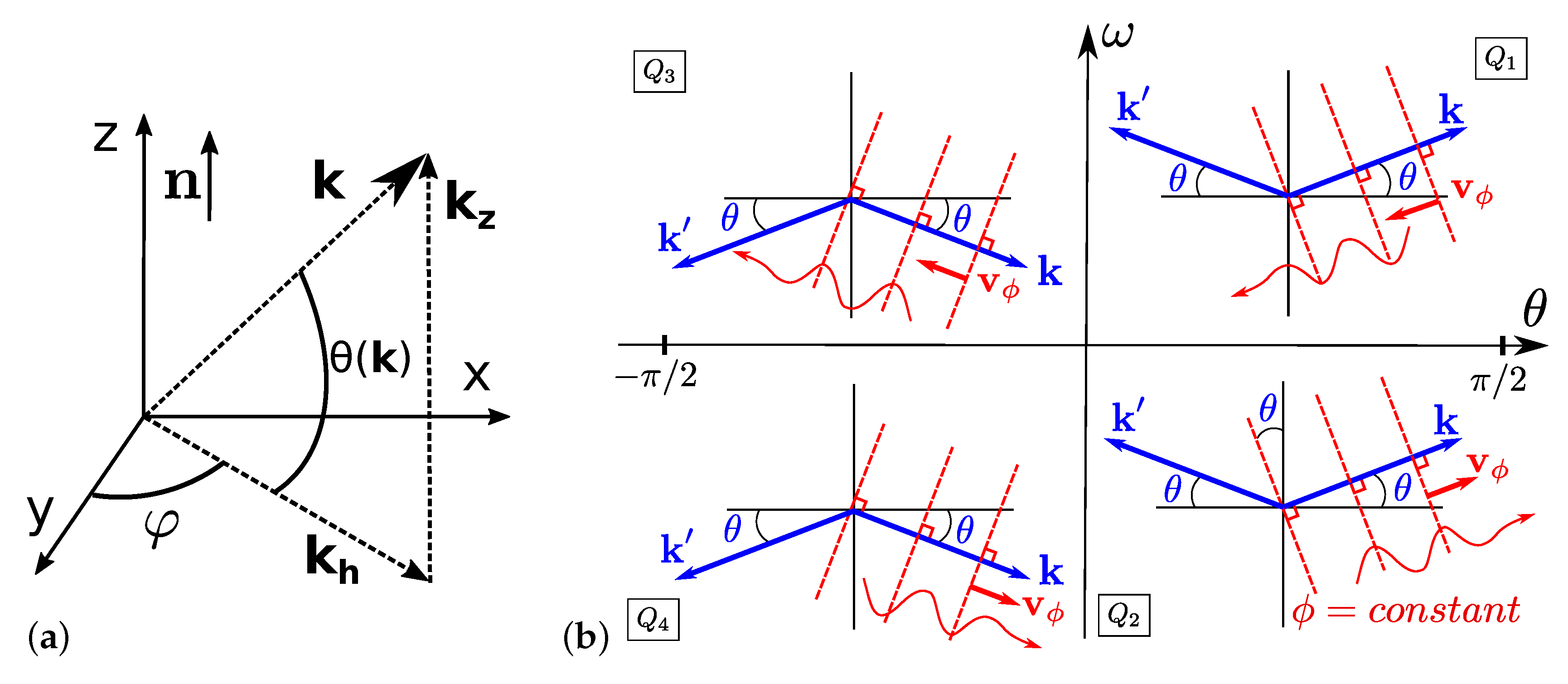
2.1. Governing Equations and Dispersion Relation

We consider the Navier–Stokes equations in the Boussinesq approximation for an incompressible fluid:

$$\begin{array}{c}{\partial }_t\mathbf{u}+\omega \times \mathbf{u}+\mathbf{\nabla }p-\nu {\mathbf{\nabla }}^2\mathbf{u}=\mathbf{n}b+{\mathbf{F}}_u\\ \mathbf{\nabla }·\mathbf{u}=0\\ {\partial }_{t}b+\mathbf{u}·\mathbf{\nabla }b-\chi {\mathbf{\nabla }}^{2}b=-N^2\mathbf{n}·\mathbf{u}+F_b\end{array}$$

(1)

where $\mathbf{u}=(u_x,u_y,u_z)$ is the velocity vector, $\omega =\nabla \times \mathbf{u}$ is the vorticity, b is the buoyancy field, p is the pressure field, ${\mathbf{F}}_u$ and $F_b$ are the external forcing, $\nu$ is the kinematic viscosity, and $\chi$ is the thermal diffusivity. $\mathbf{n}$ is a vertical unit vector for the axis that bears gravity (along the vertical direction z). The buoyancy b accounts for the fluctuation of density around the mean gradient $N^2$ where N is the Brunt–Väisälä frequency. For simplification, the Prandtl number is chosen equal to one: $Pr=\nu /\chi =1$. The fields in these equations are assumed to be non-dimensionalized by reference length and time scales.

A plane wave solution $exp\left(i\right(\mathbf{k}·\mathbf{x}+\omega t\left)\right)$ with wavevector $\mathbf{k}$ and frequency $\omega$ is obtained for the linearized Equation (1) without viscosity. Viscous dissipation can easily be re-introduced, although the inviscid solution is retained here for the sake of simplicity. From this inviscid plane-wave solution, the dispersion relation of internal gravity waves [5] can be recovered as

$${\omega }_r=\pm Ncos\theta$$

(2)

where $\theta$ is the angle of the wavevector $\mathbf{k}$ with the horizontal plane $(x,y)$ (see Figure 1a). This dispersion relation is very particular because it involves the stratification intensity N and the angle of propagation $\theta$ of the wave. Furthermore, unlike sound waves or surface waves, the dispersion relation depends only on the orientation of the wavevector $\mathbf{k}=(k_x,k_y,k_z)$ and not on its amplitude $k=\left|\mathbf{k}\right|$. We denote ${\mathbf{k}}_h=(k_x,k_y)$ the projection of $\mathbf{k}$ on the horizontal plane (see Figure 1a), and $k_h=\left|{\mathbf{k}}_h\right|$. According to Pedlosky [24], the crest of constant phase $\varphi =\mathbf{k}·\mathbf{x}+\omega t=\mathrm{constant}$ propagates perpendicularly to the wavevector $\mathbf{k}$ since ${\mathbf{\nabla }}_{\mathbf{x}}\varphi =\mathbf{k}$ with a phase velocity ${\mathbf{v}}_{\mathsf{\Phi }}=\omega \mathbf{k}/k^2$. It propagates with a phase velocity ${\mathbf{v}}_{\mathsf{\Phi }}$ parallel to $\mathbf{k}$ if $\omega <0$ and anti-parallel to $\mathbf{k}$ if $\omega >0$. In Figure 1b, we plot the four possibilities (the four quadrants $Q_1,Q_2,Q_3,Q_4$) of the propagation of the crest of phase in the plane $(\theta ,\omega )$ according to the signs of $\theta$ and $\omega$. Note that the envelope of the wave, (i.e., the energy of the waves) propagates along the direction of the group velocity ${\mathbf{v}}_g={\mathbf{\nabla }}_{\mathbf{k}}\omega$ which is perpendicular to the wavevector $\mathbf{k}$ for IGW [24].

2.2. Numerical Method

The complete nonlinear Equation (1) are non-dimensionalized and solved using a classical pseudo-spectral method [25] in a periodic domain of length $2\pi$ in each direction. The numerical domain is periodic with a grid spacing uniform and a number of grid points noted $n_g$ in the three directions ($n_g^3$ points overall). The 3D spatial Fourier transform is done with the P3DFFT library [26]. The viscous and diffusive terms are solved via an implicit treatment implemented as a change of variable involving an exponential integrating factor. The transformed variables for the velocity vector and buoyancy fields are in Fourier space:

$$\begin{array}{c}{\mathbf{u}}^{*}(\mathbf{k},t)=\mathbf{u}(\mathbf{k},t)e^{\nu k^{2}t}\\ b^{*}(\mathbf{k},t)=b(\mathbf{k},t)e^{\chi k^{2}t}\end{array}$$

(3)

thus reducing a possible numerical approximation error for diffusion. The dealiasing of the quadratic terms is based on the phase shifting method [27] with a truncation at $k_{max}=\sqrt{2}(2/3)k_N$ with the Nyquist wavenumber $k_N=n_g/2$. A third-order Adams–Bashforth time-scheme is used to perform numerical time integration. The code is parallelized using MPI. Simulations are done either in the laminar case or in the turbulent case. In the laminar case, a specific forcing ${\mathbf{F}}_u$ and $F_b$ is chosen which is explained case-by-case in the next sections. In the turbulent case, a specific spectral statistical forcing (explained in [28]) is used, with the advantage of limiting the increase of VSHF. It consists in forcing velocity only ($F_b=0$) with a forcing term ${\mathbf{F}}_u$ chosen in Fourier space to ensure a constant injected power $P=<{\mathbf{F}}_{\mathbf{u}}·\mathbf{u}>$, where $<*>$ is a statistical volume average. The force ${\mathbf{F}}_u$ is applied in a cylindrical shell of radius $k_v$ with finite vertical extent between $k_{v,min}$ and $k_{v,max}$. The mesh size is chosen to ensure accurate resolution of the smallest scales through the condition $k_{max}\eta \simeq 1$, where $k_{max}$ is the maximum resolved wavenumber, $\eta ={({\nu }^3/\epsilon )}^{1/4}$ is the Kolmogorov length scale and $\epsilon$ is the kinetic energy dissipation. The space-time evolution of the velocity and density fields are then post-processed to obtain various statistics, as in Section 2.3.

2.3. Space-Time Analysis of the Flow

Space-time statistics are computed to link the direction of propagation $\theta$—a spatial variable—to the frequency $\omega$—a time variable. This is done by calculating the time-dependent angular-dependent spectral density of kinetic energy. To do this, the wavevector space is first decomposed into different elementary cones with an angle $\theta$ with respect to the horizontal plane and a length k (see Figure 2). Due to the $\theta$ angle discretization, the elementary cone is a thin volume where all wavevectors $\mathbf{k}$ have an angle $\theta \left(\mathbf{k}\right)\in I_{\theta }=[\theta -\Delta \theta ,\theta -\Delta \theta ]$. To compute the energy into this elementary cone, we decompose the computation into four steps:

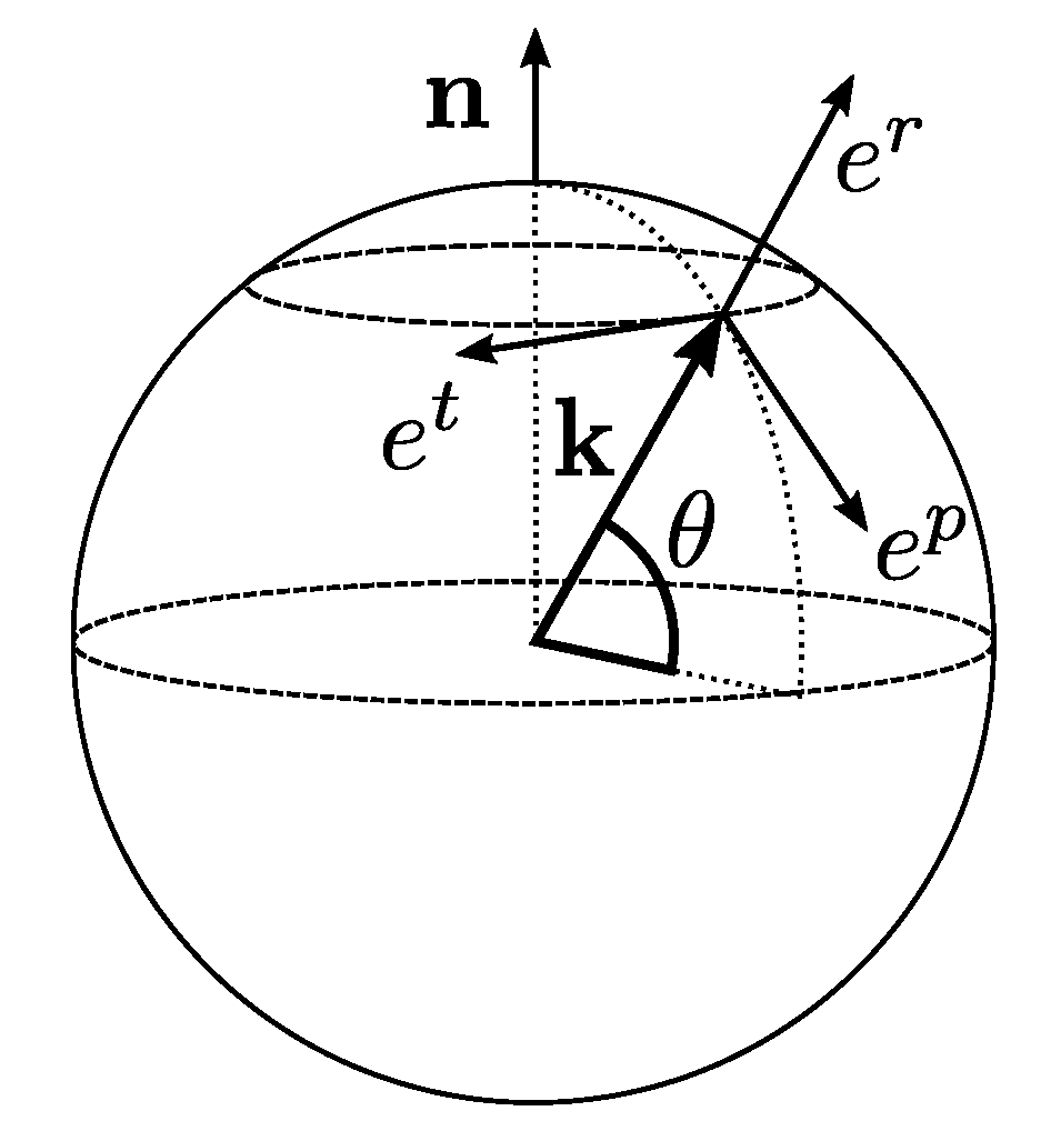
• Each elementary cone, which contains wavevector $\mathbf{k}$ with an angle $\theta \left(\mathbf{k}\right)\in I_{\theta }$, is divided into sub-volumes by selecting the scale $k=\left|\mathbf{k}\right|$. Then, all the velocity vectors are summed onto the sub-volume in a new variable $\mathbf{U}(\theta ,t,k)={\displaystyle \sum _{\theta \left(\mathbf{k}\right)\in I_{\theta },\left|\mathbf{k}\right|=k}}\mathbf{u}(\mathbf{k},t)$.
• The Fourier transform in time of that new variable is computed as $\tilde{\mathbf{U}}(\theta ,\omega ,k)=\mathit{TF}\left[\mathbf{U}(\theta ,t,k)\right]$.
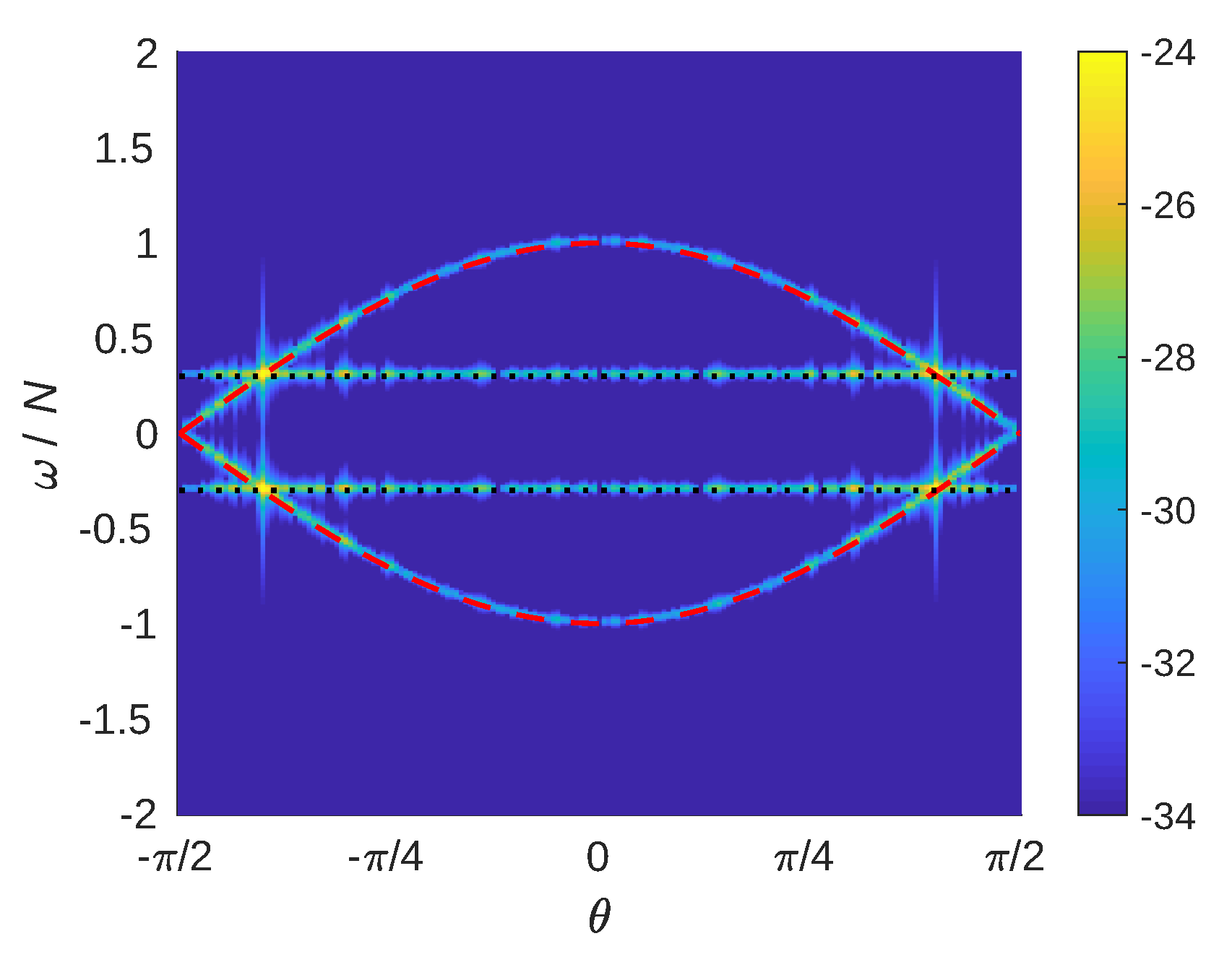
• The spectral density of kinetic energy is recovered in a $(\theta ,\omega )$ plane for a range of scales between $k_1$ and $k_2$ that is a set of sub-volumes:

  $$E(\theta ,\omega ,k_1\le k\le k_2)=\sum _{k_1\le k\le k_2}E(\theta ,\omega ,k)=\sum _{k_1\le k\le k_2}{\left|\tilde{\mathbf{U}}(\theta ,\omega ,k)\right|}^2.$$

  (4)
• The total spectral density of kinetic energy into an elementary cone, regardless of scale k, can be computed as a summation over all sub-volumes:

  $$E(\theta ,\omega )=\sum _{0\le k\le k_{max}}E(\theta ,\omega ,0\le k\le k_{max}).$$

  (5)

When the numerical simulation contains only waves, one should observe a peak of energy density that follows the dispersion relation curve defined by Equation (2) in the $(\theta ,\omega )$ plane (as illustrated in Figure 3b). We detail this in Section 2.4.

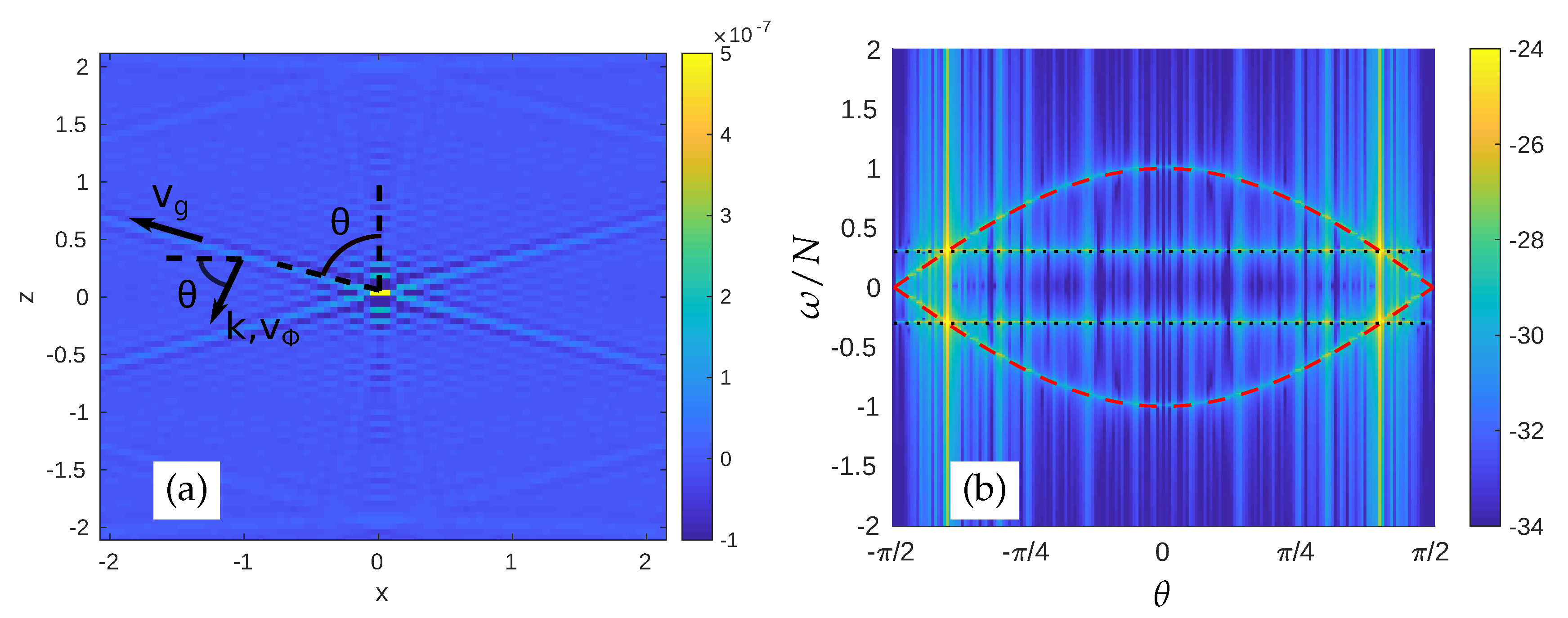
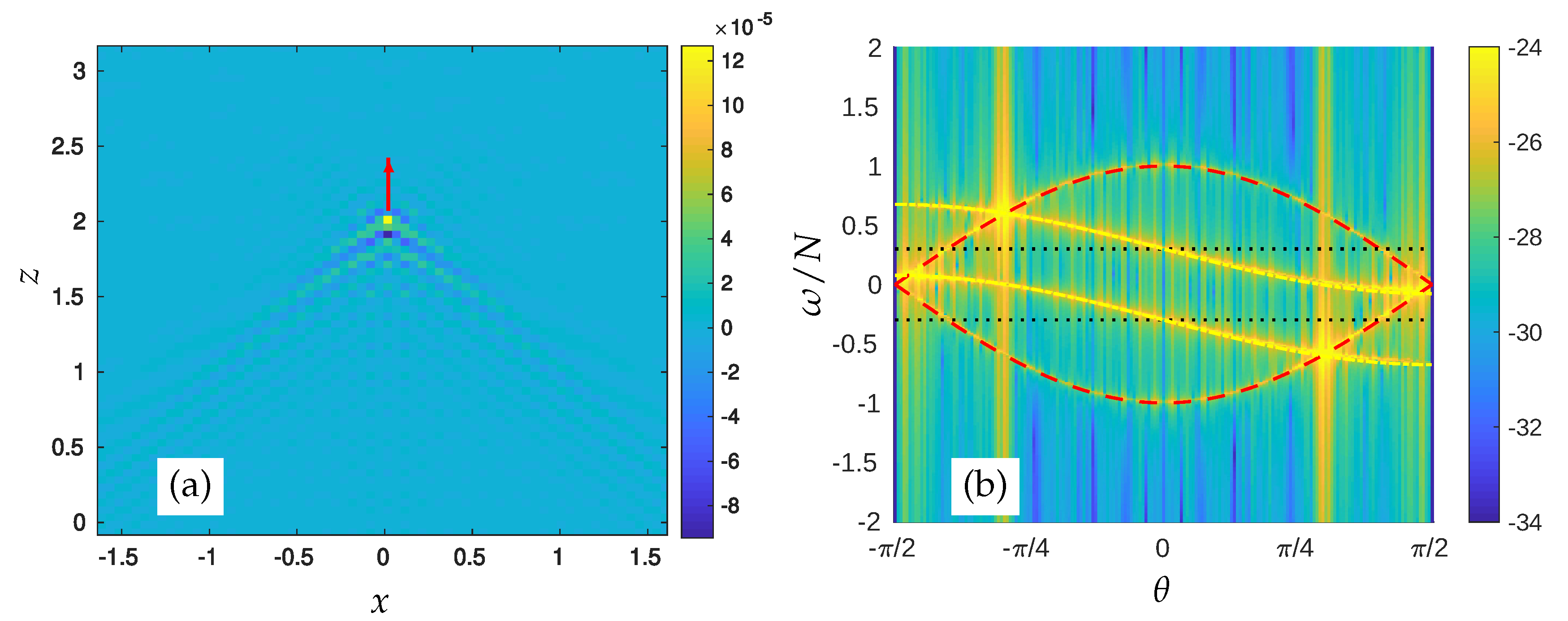
2.4. Saint Andrews cross Wave Propagation Benchmark

We test here the statistical characterization of waves by a simple benchmark consisting of a single wave propagation in a Saint Andrew cross pattern, as in experiments [5]. The flow forcing produces only waves and is examined from its initial condition at rest. Several forcing possibilities exist to create either a single isolated wave or several superimposed ones. The forcing term is introduced in the linearized Navier–Stokes equations in the Boussinesq approximation: the non-linear terms $\mathit{\omega }\times \mathbf{u}$ and $\mathbf{u}·\mathbf{\nabla }\mathbf{b}$ are removed from Equation (1), likewise in the numerical simulation. For this benchmark, the forcing $F_b$ is only imposed in the buoyancy equation, so that $F_u=0$. We choose a point forcing localized in physical space, of the form:

$$F_b={\delta }_{x}sin\left({\omega }_{f}t\right)$$

(6)

with ${\omega }_f=0.3$. This forcing implemented only in the buoyancy equation of system Equation (1) ensures that the incompressibility condition is maintained for the velocity field. The function ${\delta }_x$ is the Dirac function. In the Fourier space, it means that all wavenumbers are forced even though there is more energy for high wavenumbers.

We use this forcing in a simulation without non-linear terms. The resolution is $n_g=128$, we assume negligible viscous diffusion so that $\nu ={10}^{-7}$, and the Brunt–Väisälä frequency is $N=1$. As expected, we observe in Figure 3 the propagation of waves according to an angle $\theta$ set by ${\omega }_f$ such that ${\omega }_f=Nsin\theta$. Figure 3a shows the distribution of the vertical velocity components, and the same pattern is observed in the buoyancy field (not shown). The spatiotemporal analysis is then applied using 1000 fields separated by a time step $\Delta t=0.5$. The total time span is therefore $79.6T_N$ where the $T_N=2\pi /N$ is the Brunt–Väisälä period. Upon computing the space-time statistics of energy density $E(\theta ,\omega )$ according to Equation (5), the energy distribution in the $(\theta ,\omega )$ plane (Figure 3b) appears to concentrate in two kinds of regions: (a) along two horizontal lines of energy concentration, at ${\omega }_f=\pm 0.3$ (these lines are the traces in the numerical simulation of the pointwise spatial forcing—almost a Dirac—that oscillates at frequency ${\omega }_f$, which is Fourier transformed); and (b) along the dispersion relation curves (in absence of non-linearity, no energy redistribution can occur away from the immediate input due to the forcing). Both kinds of energy concentration curves correspond to the response of the linear system to the forcing, with one component at its forcing frequency ${\omega }_f$ and one at the natural frequency of the system, which is here the frequency of the waves ${\omega }_r$. The maximum of $E(\theta ,\omega )$ is therefore observed at the crossing points of the forcing and the dispersion relation curves, that is at $\theta \simeq 72.5°$. In physical space, this peak energy results in the observation in of waves propagating at $\theta \simeq 72.5°$, which is indeed what we measure in Figure 3.

This numerically observed solution of the response of the linearized system of equations to harmonic forcing is computed analytically in Appendix B from the inviscid Navier–Stokes–Boussinesq equations with a zero initial condition. The analytical solution for the buoyancy field is:

$$\overline{b}\left(\omega \right)=\frac{{\omega }_f}{{\omega }_r^2-{\omega }_f^2}\left[\frac{\delta (\omega -{\omega }_f)+\delta (\omega +{\omega }_f)}{2}-\frac{\delta (\omega -{\omega }_r)+\delta (\omega +{\omega }_r)}{2}\right].$$

(7)

From this solution, two regions of concentration of energy can indeed be found: one along the line defined by $\omega =\pm {\omega }_f$, which is the frequency of the forcing, and one along the curve $\omega =\pm {\omega }_r$, which is the frequency of the waves along the dispersion relation. This solution diverges for ${\omega }_f=\pm {\omega }_r$ because it is an inviscid solution, but it shows that the maximum of energy is at the intersection of these frequencies.

Note that several vertical lines at constant angle $\theta$ are visible in Figure 3b in a log-scale. Each line based on constant $\theta$ corresponds to an independent set of Fourier transforms in time. We think that there are two main numerical reasons for these vertical lines. Firstly, numerically, the Dirac function in Equation (7) is replaced by a sinc function, with visible effect in log scale. Secondly, we do not use any windowing technique because it introduces an artificial coefficient that changes the energetic ratio between the dispersion relation and the input signal. This would make difficult to filter the waves from the eddies as done in Section 4. To remain consistent with the rest of the article, we do not apply a windowing technique (such as Hann) and we analyze the raw data. Nevertheless, in Appendix A, we apply this technique on the same data as in Figure 3b: this technique increases the concentration of energy around the dispersion relation. Moreover, this vertical line tends to disappear when the four-dimensional filtering is used (see Section 4.2) or when statistical stationarity is reached (see Section 4.6).

3. Sweeping and Doppler Effects on Internal Gravity Waves Propagation

We show above that the dispersion relation can be recovered accurately from a space-time statistical analysis of a simple flow where a single wave propagates, as shown in Figure 3. However, in more complex flows, waves can be convected by eddies, by a mean shear or by any other kind of large-scale flow. To understand how the frequency of the waves can be modified, and how this translates into a new pattern of energy $E(\theta ,\omega )$ concentration in $(\theta ,\omega )$ plane, we consider a mean flow homogeneous—i.e., periodic—in one spatial direction, and we compute its effect on internal gravity waves propagation.

The reader can find an overview of our simulation cases in

Table 1. List of numerical parameters for the different numerical simulations presented in this paper.

Section	Dispersion Relation	Forcing Frequency	Advective Velocity	N	$\mathit{\nu }$
Section 2.4	$Ncos\theta$	$0.3$	none	1	${10}^{-7}$
Section 3.1.2	$Ncos\theta +c_{z}ksin\theta$	$0.3$	$c_z={10}^{-2}$	1	${10}^{-7}$
Section 3.1.3 and Section 4.2	$Ncos\theta +c_{x}kcos\theta sin\phi$	$0.3$	$c_x={10}^{-2}$	1	${10}^{-7}$
Section 3.2	$Ncos\theta$	$0.3+c_{z}ksin\theta$	$c_z=6.28\times {10}^{-3}$	1	${10}^{-7}$
Section 3.3	$Ncos\theta +{\mathbf{u}}_{shear}({\mathbf{k}}_h=0,k_z=\pm 1)·\mathbf{k}$	$0.5$	$max\left(\right|{\mathbf{u}}_{shear}\left|\right)=0.01$	1	${10}^{-7}$
Section 4.3, Section 4.4, Section 4.5, Section 4.6, Section 4.7 and Section 4.8	$Ncos\theta +\mathbf{c}·\mathbf{k}$	none	$\mathbf{c}=(0.14,0.14,0)$	5	$1/2500$

that gathers the main parameters for the laminar cases and the turbulent case. Results for the turbulent case are presented in Section 4.3.

3.1. Sweeping by a Uniform Convective Flow

To begin with, we consider the case of a uniform convective flow with mean velocity vector either in the vertical direction—i.e., along the axis of propagation symmetry—or the horizontal direction—perpendicular to the axis of propagation symmetry. The sweeping effect of the flow is then characterized for both cases from both theoretical and numerical predictions.

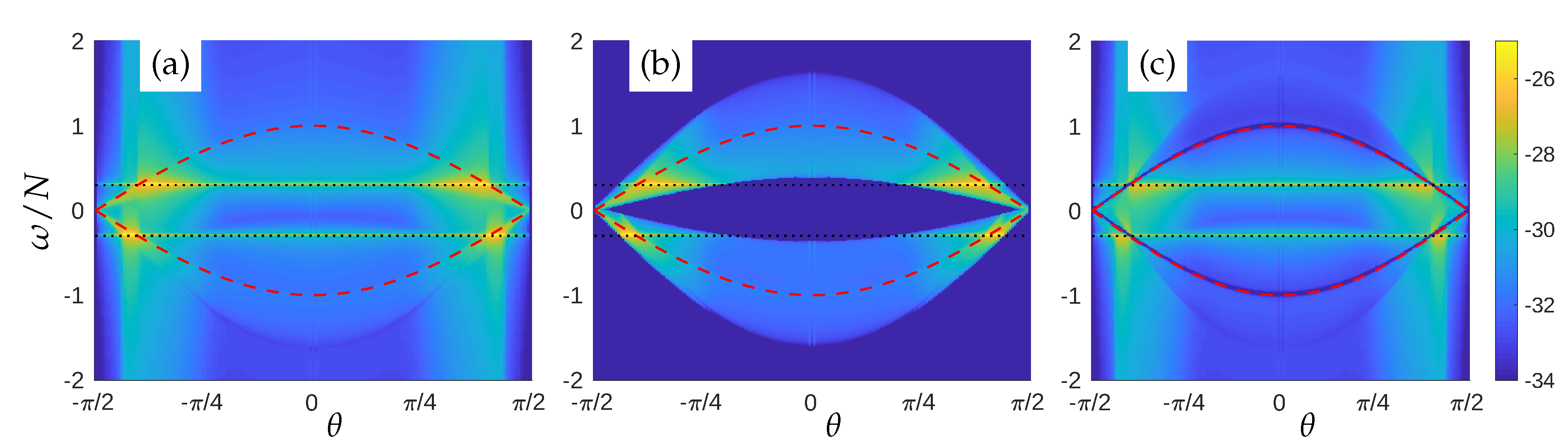
3.1.1. Theoretical Modified Dispersion Relation

The advecting mean flow $\mathbf{c}=(c_x,0,c_z)$ is introduced in the Navier–Stokes–Boussinesq equations as follows:

$$\begin{array}{c}{\partial }_t\mathbf{u}+\mathbf{c}·\mathbf{\nabla }\mathbf{u}=-\mathbf{\nabla }p+\nu {\mathbf{\nabla }}^2\mathbf{u}+\mathbf{n}b\\ {\partial }_{t}b+\mathbf{c}·\mathbf{\nabla }b=\chi {\mathbf{\nabla }}^{2}b-N^2\mathbf{n}·\mathbf{u}+F_b\end{array}$$

(8)

Since the mean flow is uniform, the convection term can be introduced in the numerical simulation via a change of variable (similar to that for diffusion in Equation (3)) where the new velocity vector and buoyancy fields are:

$$\begin{array}{c}{\mathbf{u}}^{*}(\mathbf{k},t)=\mathbf{u}(\mathbf{k},t)e^{\nu k^{2}t+\mathrm{i}\mathbf{c}·\mathbf{k}t}\\ b^{*}(\mathbf{k},t)=b(\mathbf{k},t)e^{\chi k^{2}t+\mathrm{i}\mathbf{c}·\mathbf{k}t}.\end{array}$$

(9)

With this new set of linearized equations, the inviscid dispersion relation becomes ${\omega }^{\prime }=\omega +\mathbf{c}·\mathbf{k}$, which shows that the wave deviation is larger at large wavenumber k. This new dispersion relation can easily be found by using a change of variable in the time and the spatial Fourier domains. According to Figure 1b, a kinematic analysis permits to infer the variation of the frequency in function of the advective flow $\mathbf{c}$: when $\mathbf{c}$ is in the same direction as the phase velocity (see Figure 1b), the angular frequency increases, whereas, when $\mathbf{c}$ is in the opposite direction of the phase velocity, the angular frequency decreases. Such a modification of the dispersion relation was already observed in a rotating flow experiment, although indirectly: measurements of a Doppler-like frequency shift were explained by taking into account sweeping by the two-dimensional geostrophic mode observed in the turbulent fluid tank [29].

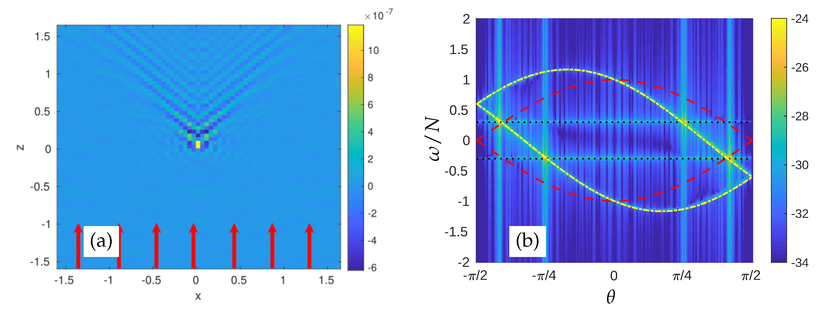
3.1.2. Sweeping by Vertical Velocity

We start by considering a vertical advecting velocity field $\mathbf{c}=(0,0,c_z)$, i.e., along the natural axis of symmetry of the system, borne by the gravity vector. The Saint Andrew’s cross pattern obtained without mean flow as in Section 2.4 is therefore convected towards positive z direction. As a result, the dispersion relation is modified by the term $\mathbf{c}·\mathbf{k}=c_z{k}_z=c_{z}ksin\theta$:

$${\omega }^{\prime }={\omega }_r+c_{z}ksin\theta$$

(10)

The result is shown in the two panels of Figure 4 for $c_z={10}^{-2}$, with the same physical and numerical parameters as in Section 2.4. Figure 4a shows that the wave-packet is translated, thus producing a ‘wake-like’ pattern, much as that of a uniformly propelled boat for surface waves. Figure 4b shows the distribution of energy density $E(\theta ,\omega )$. This figure shows that the dispersion relation is modified according to Equation (10), and that maximum modification is observed when considering the largest wavenumber range $56<k\le k_{max}=60$. This domain of wavenumber is chosen in order to observe the maximum effect of the sweeping effect. Moreover, the energy density $E(\theta ,\omega ,56<k\le 60)$ gets very large at the intersection between the forcing and the modified dispersion relation with an asymmetrical angle value of $\theta \simeq \pm 0.8\mathrm{rad}$ and $\theta \simeq \pm 1.3\mathrm{rad}$. Note that Figure 4b is in agreement with Figure 1b: in quadrant $Q_1$, $\mathbf{c}$ is in the opposite direction compared to the vertical component of phase velocity ${\mathbf{v}}_{\varphi }$, and the frequency $\omega$ decreases compared to the dispersion relation. In quadrant $Q_2$, a similar kinematic reasoning leads to an increase of the angular frequency $\omega$. This reasoning could be extended to quadrants $Q_3$ and $Q_4$.

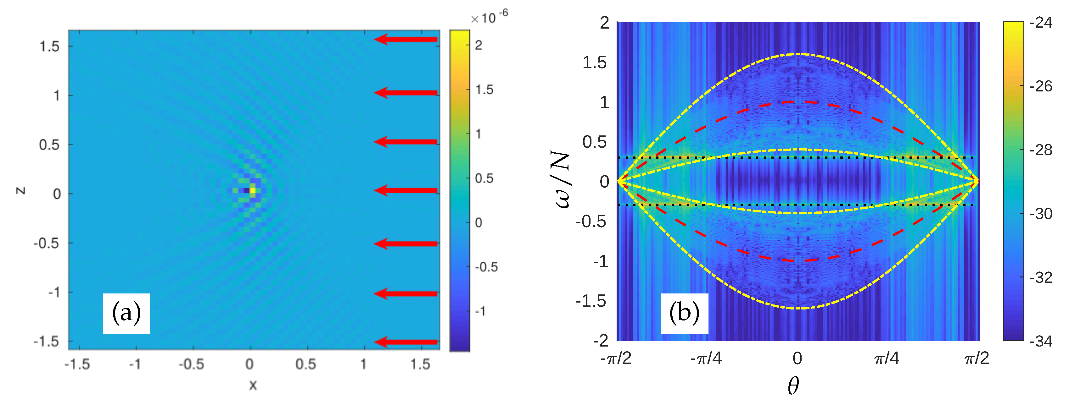
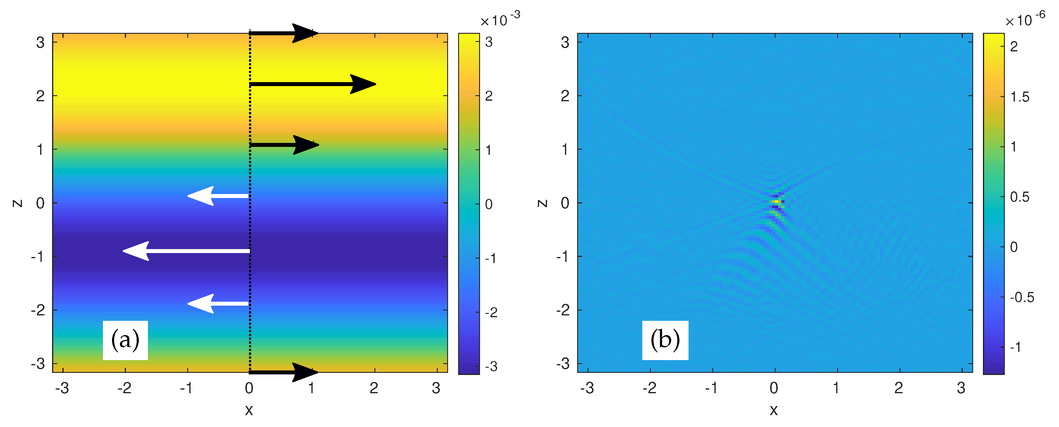
3.1.3. Sweeping by Horizontal Velocity

In this second case of uniform background flow, we consider a horizontal convecting velocity field $\mathbf{c}=(c_x,0,0)$. The wave propagation is therefore convected to the negative x direction, and the initial vertical axisymmetry of the flow is broken. As a result, the dispersion relation is observed in Figure 5 to be modified proportionally to $\mathbf{c}·\mathbf{k}=c_x{k}_x$.

Unlike the case of vertical convecting velocity, the sweeping effect of horizontal convection velocity cannot be computed by an exact analytical solution in the $(\omega ,\theta ,k)$ plane. It can only be estimated within an interval between the minimum and maximum of the analytical dispersion relation. This is because the azimuthal angle $\phi$ is discarded when computing the energy density in Equation (5), due to the fact that the projection of the wavevector $\mathbf{k}$ along the x axis is $k_x=kcos\theta sin\phi$ (see Figure 1a). At fixed radial angle $\theta$ and fixed wavenumber k, all angles $\phi =0\cdots 2\pi$ are selected and thus $k_x$ may vary from 0 to $k_h$. The region within which the frequency ${\omega }^{\prime }$ is found therefore lies between two boundaries:

$${\omega }_r-c_{x}kcos\theta \le {\omega }^{\prime }={\omega }_r+c_{x}kcos\theta sin\phi \le {\omega }_r+c_{x}kcos\theta .$$

(11)

The modified Saint Andrew’s cross pattern advected by a horizontal velocity $c_x=-{10}^{-2}$ is shown in Figure 5a for the same physical and numerical parameters as in Section 2.4. In physical space, Figure 5a shows that the wave packet propagation pattern is different from that of the vertical velocity case (Figure 5b): the flow being axisymmetric along the axis of gravity, a sweeping velocity in the vertical direction preserves this symmetry, but horizontal sweeping breaks it. In frequency space, Figure 5b shows the distribution of energy density $E(\theta ,\omega )$: zones of maximum energy indicate that the dispersion relation is modified consistently with the above-mentioned enveloping region defined in Equation (11), with maximum modification with respect to the dispersion relation when $56<k\le k_{max}=60$. In addition, we note that the intersection between the forcing frequency horizontal line and the enveloping region, the energy density $E(\theta ,\omega ,56<k\le 60)$ blows up, indicating maximal response of the linear system dynamics. Note that Figure 5b is in agreement with Figure 1b: in quadrant $Q_1$, $\mathbf{c}$ is in same direction compared to the horizontal component of the phase velocity ${\mathbf{v}}_{\varphi }$ for the wavevector $\mathbf{k}$, and then the frequency $\omega$ increase compared to the dispersion relation by a factor that depends on the alignment of ${\mathbf{v}}_{\varphi }$ with $\mathbf{c}$, i.e., the azimuthal angle $\phi$. The same reasoning applied to the wavevector ${\mathbf{k}}^{\prime }$ leads to a decrease in the frequency $\omega$ compared to the dispersion relation ${\omega }_r$. Therefore, in quadrant $Q_1$, the frequency of the waves surrounds the dispersion relation ${\omega }_r$. The same kinematic reasoning can be done for quadrants $Q_2$, $Q_3$ and $Q_4$.

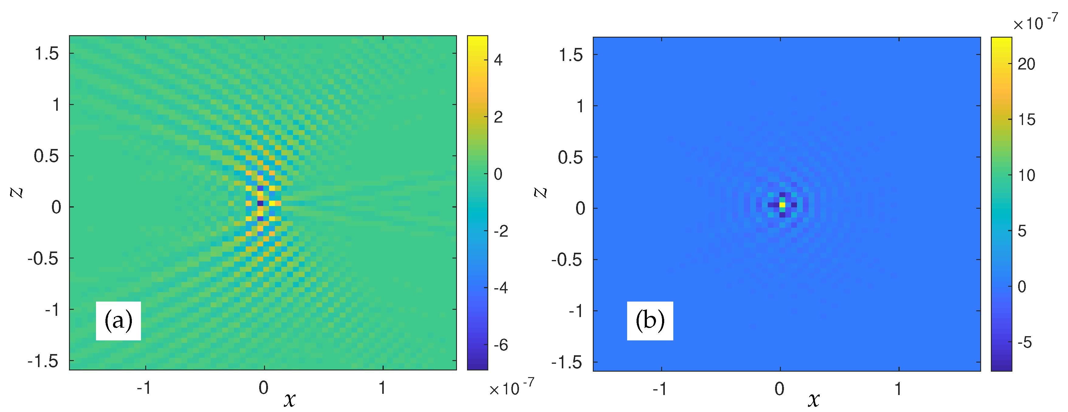
3.2. Doppler Shift Due to the Motion of the Wave Source

In Section 3.1, we consider how the wave frequency could be modified by the presence of a convective velocity. We now investigate a reversed configuration in which the wave production mechanism moves at a constant velocity, and in which the modification of the dispersion curve could be different. This new configuration is simulated using a forcing $F_b$ modified so that it is spatially phase-shifted, which, in practice, is done in Fourier space. In physical space, the forcing is thus advected at constant vertical velocity $c_z$. The new forcing is therefore:

$$F_b={\delta }_{\mathbf{x}-{\mathbf{c}}_{z}t}sin\left({\omega }_{f}t\right)$$

(12)

with ${\omega }_f=0.3$ and we choose $c_z=6.28\times {10}^{-3}$.

In Figure 6a, in the physical vertical plane, the local forcing can be seen to move in the positive z direction in physical space for the same physical and numerical parameter as in Section 2.4. The wave seems to be similar to the case of the sweeping effect with vertical velocity of Figure 4a, with an opposite direction of propagation.

In the Fourier domain, the dispersion curve is not modified, but only the forcing frequency ${\omega }_f$ is modified by addition of the correction $\mathbf{c}·\mathbf{k}=c_{z}ksin\theta$. It is modified similarly to the sweeping effect as the new forcing frequency (dash-dotted yellow curve in Figure 6b) is equal to

$${\omega }_f^{\prime }={\omega }_f+c_{z}ksin\theta .$$

(13)

Therefore, unlike the sweeping effect, the Doppler effect does not modify the frequency of internal gravity waves and the original dispersion relation is preserved. This is shown in Figure 6b, where the dispersion relation Equation (2) is not modified (red dashed curve), whereas the forcing frequency is modified according to Equation (13) for a wavenumber amplitude between $56<k<k_{max}=60$. At the crossing between the two curves indicating the modified frequency of forcing and the dispersion relation, the concentration of energy density $E(\theta ,\omega )$ is maximal at $(\theta ,\omega )=(-1.5,0.1)$ and $(-0.9,0.6)$, and their symmetries with respect to the $(0,0)$ point are at $(0.9,-0.6)$ and $(1.5,-0.1)$

3.3. Sweeping by a Sheared Convective Mean Flow

The propagation of waves convected by a large-scale non uniform flow is considered here. In a stratified flow, a large scale shear flow can often dominate the overall structure of the flow, and evolves slowly in time. It is called the Vertically Sheared Horizontal Flow (VSHF). This shear flow is characterized by vertical variation only, without vertical velocity. This strong vertical shearing depends only on a vertical wavevector (i.e., $k_h=0$), so that the velocity $u_{shear}(k_h=0,k_z)$ is parallel to the horizontal plane and the dispersion relation gives a frequency $\omega =0$ (see [30]). This VSHF mode is not considered as a wave and the perturbation density distribution b in this case is uniformly zero. Therefore, these large-scale non-uniform flows are often the dominant sources of sweeping of internal gravity waves. This mode has generally been observed in numerical simulations, either in forced turbulence [30,31,32] or in decaying turbulence [33], as well as in statistical approaches such as EDQNM models [21] or the statistical state dynamics [12]. Moreover, VSHF appear in strongly stratified turbulence (low Froude number and high buoyancy Reynolds number) and not in weak stratification (high Froude number) [34]. In the context of geophysical fluid dynamics, the VSHF is an ageostrophic horizontal wind and can help to understand the emergence and maintenance of some turbulent jets, such as banded winds of Jupiter or equatorial deep jets of ocean by an interaction between wave and mean flow [35]. Nevertheless, the formation of VSHF is not really understood in many ways. Several theories try to explain the mechanisms of VSHF’s formation, such as resonant interactions among gravity wave [30,32], rapid distortion theory [36] and recently by a linearized version of statistical state dynamics [12]. It appears that the VSHF is fed by an interaction with small scales of turbulence, so that a minimum rate of turbulence is required. To quantify the effect of the VSHF mode on the dispersion relation and on the internal gravity waves propagation, our method is to proceed in two stages.

In the first stage, the VSHF flow is obtained from a direct numerical simulation of the linearized Navier–Stokes–Boussinesq Equation (1). The VSHF mode is directly forced using a stochastic forcing of velocity explained in [28]. The force is only imposed on the velocity component ${\mathbf{F}}_u({\mathbf{k}}_h=0,k_z)$ with $k_z=\pm 1$ and an injected power $P=<{\mathbf{F}}_u·\mathbf{u}>={10}^{-6}$; as a result, the forcing only operates on the large-scales of the flow. The obtained VSHF is a solution of the linearized Equation (1). Figure 7a shows the distribution in the $(x,z)$ vertical plane of physical space of the horizontal component $u_{shear,x}$ of velocity ${\mathbf{u}}_{shear}=(u_{shear,x},u_{shear,y},0)$.

In the second stage, the amplitude of the VSHF flow is chosen to produce a significant sweeping effect although without totally drowning the original dispersion relation. This ad hoc adjustment permits to observe the qualitative effects of VSHF sweeping on internal waves propagation, but should eventually be related to physical observation or experimental data for better quantification. In the following, the shear velocity ${\mathbf{u}}_{shear}$ is increased by $2.5$ to obtain a maximum for the horizontal shear velocity norm of $max\left(\right|{\mathbf{u}}_{shear}\left|\right)=0.01$.

We then consider the flow containing the obtained VSHF mode ${\mathbf{u}}_{\mathrm{shear}}$, and its linear dynamics is numerically solved using the following linearized Navier–Stokes–Boussinesq equations:

$$\begin{array}{c}{\partial }_t\mathbf{u}+\omega \times {\mathbf{u}}_{shear}+{\omega }_{shear}\times \mathbf{u}=-\mathbf{\nabla }p+\nu {\mathbf{\nabla }}^2\mathbf{u}+\mathbf{n}b\\ {\partial }_{t}b+{\mathbf{u}}_{shear}·\mathbf{\nabla }b=-\chi {\mathbf{\nabla }}^{2}b-N^2\mathbf{n}·\mathbf{u}+F_b\end{array}$$

(14)

where ${\omega }_{\mathrm{shear}}=\mathbf{\nabla }\times {\mathbf{u}}_{\mathrm{shear}}$ is the mean vorticity induced by the VSHF.

Equation (14) is solved numerically with a resolution $n_{grid}=128$ grid points in each space direction, $\Delta t=0.25$, $\nu ={10}^{-7}$, ${\omega }_f=0.5$, and by using a point forcing as in Section 2.4. The simulation is started from fluid at rest, and, from this initial time on, statistics are accumulated, so that the analyzed dataset is composed of 3000 velocity–buoyancy fields equally spaced in time over $119.4T_N$ where $T_N=2\pi /N$ is the Brunt–Väisälä period.

In Figure 7b, the cross-shaped propagation pattern is distorted and does not follow a straight propagation line. The direction of propagation of the wave changes along with the advection velocity it encounters locally. This shows that the frequency of the waves is modified along its propagation resulting in a different angle of iso-velocity lines.

In Figure 8, the dispersion relation is clearly modified due to the VSHF mode both in the small wave number range $16<k\le 20$ (Figure 8a) and in the large wavenumber range $56<k\le 60$ (Figure 8b). On these plots, we also indicate an estimation of the sweeping effect amplitude based on the product of the amplitude of the maximum shear velocity vector with the wavevector $\mathbf{k}$, in the region described by the following two boundaries:

$$\begin{array}{ccc}\hfill {\omega }_r-c_{x}kcos\theta -c_{y}kcos\theta & \le {\omega }^{\prime }={\omega }_r+{\mathbf{u}}_{shear}·\mathbf{k}& \le {\omega }_r+c_{x}kcos\theta +c_{y}kcos\theta \hfill \end{array}$$

(15)

where the convective velocity is $c_x=rms\left(u_{shear,x}\right)$ and $c_y=rms\left(u_{shear,y}\right)$.

According to Figure 8, a concentration of energy can be found at the intersection of the wave frequency and the modified dispersion relation, at both large-scales ($16<k<20$) and small scales ($56<k<60$). To conclude, there is an amplification of forcing within the region defined by Equation (15): the larger is the wavenumber amplitude k, the larger is the sweeping effect. Moreover, the wave frequency, estimated by the sweeping effect only, seems to be in good agreement with the wave frequency observed in the simulation, notwithstanding the neglect of the effects of the term $\mathit{\omega }\times {\mathbf{u}}_{shear}+{\mathit{\omega }}_{shear}\times \mathbf{u}$ in the modification of the dispersion relation. This suggests that the sweeping effect is the main source of modification of wave frequency. Therefore, to estimate the wave frequency in a fully turbulent flow, one might simply estimate the value of the advective velocity responsible of the sweeping effect.

4. Explicit Space-Time Decomposition for Disentangling Waves and Eddies

4.1. Four-Dimensional Filtering

As mentioned in the Introduction, the classical method of decomposing stratified flows between “waves” and “vortices” [17] is a spatial decomposition. This method assumes that vortices are only on horizontal plane (in the toroidal direction), whereas waves are only in the poloidal direction (see Figure A2). This is true for a linear problem, where only the dispersion relation frequency is excited in the poloidal direction. Nevertheless, for a complete non-linear problem, the poloidal component contains some eddy motion, which has a different frequency from the dispersion relation frequency. Therefore, according to this method, they are considered as “waves” for all frequencies of the poloidal component, even those outside the dispersion relation. In that case, the explicit time dependence of velocity modes must be taken into account to discriminate waves from turbulent motion. In this case, a part of the poloidal component is considered to be an eddy part, and they are now able to vertically overturn the density field as opposed to the toroidal component. For that, a first solution is proposed in Section 3. The method of detection of waves exposed and illustrated in Section 3 is based on reduced statistics to obtain the spectral distribution of energy in $\theta$ and $\omega$. The cost of this method is limited, and it provides a first indication of the amount of wavy motion in the flow.

If one wishes to proceed to a more advanced decomposition, the solution is therefore to compute the complete space-time transforms of velocity–buoyancy fields, and to rely on this detailed information for estimating the space-time coherence of motion and thus detect the presence of wave packets. This is what we call 4D analysis, because four-dimensional transformations are required: three dimensions for space and one dimension for time. The main idea of our decomposition is to filter in Fourier space what we call “waves” by selecting the Fourier modes corresponding to the expected modified dispersion relation of internal gravity waves. The remaining part of the flow field shall be considered as “vortices”, or more broadly as eddy turbulence, and from here on we call it “eddy” to distinguish with the previous classical wave–vortex decomposition by Riley et al. [17]. Note that the dispersion relation is modified by a unique sweeping velocity in the laminar case (see previous Section 3.1), whereas, in the turbulent case, there is a continuum of sweeping velocities that we assume to vary between $-\mathbf{c}$ and $+\mathbf{c}$. It is not easy to estimate a relevant velocity $\mathbf{c}=(c_x,c_y,c_z)$ which is representative of the sweeping effect in the three spatial directions. We detail this estimation in Section 4.4. The algorithm for the new wave-eddy decomposition is detailed hereafter in five steps (see also schematic in Figure A3):

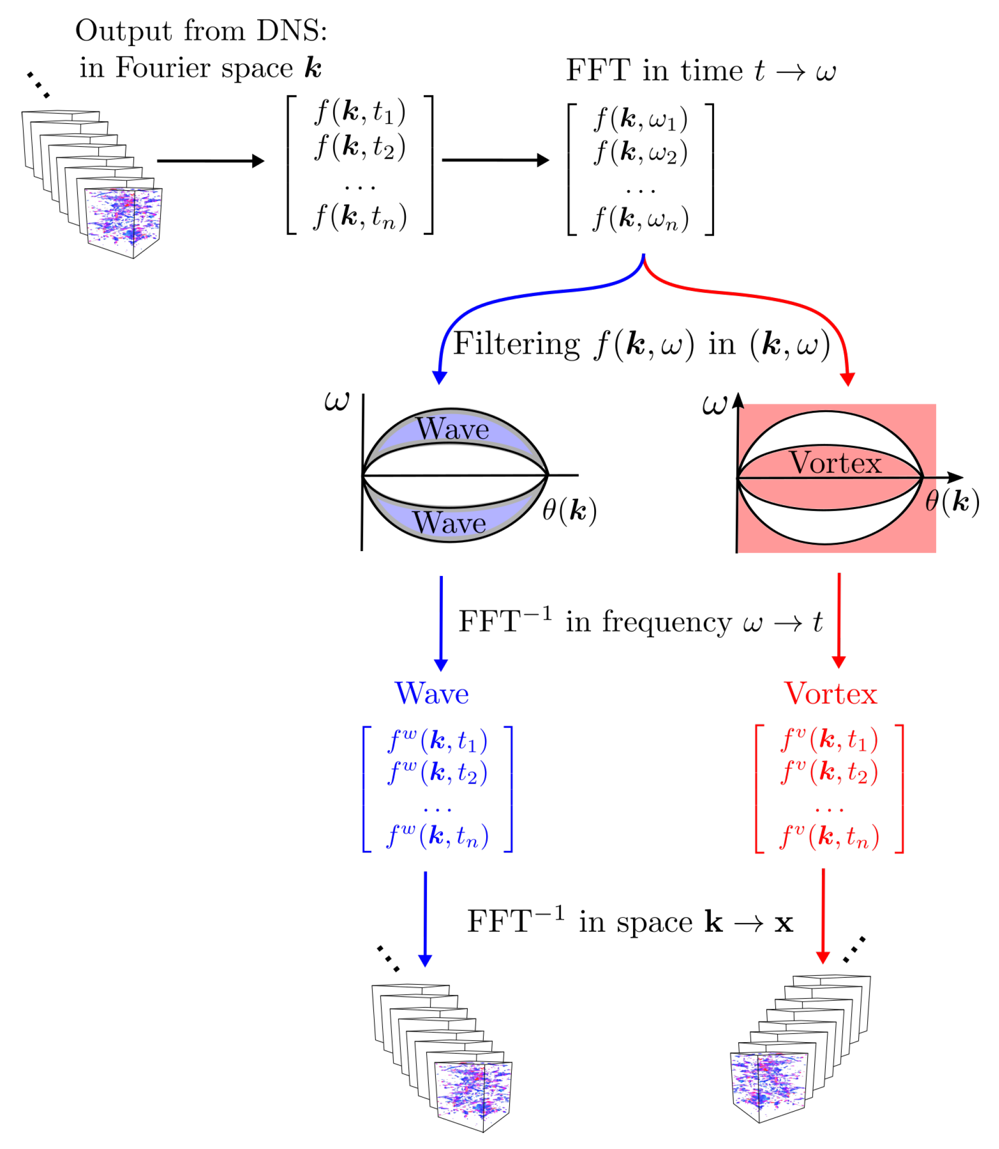
• Direct Numerical Simulation (DNS) provides time-dependent velocity–buoyancy spectral coefficients in 3D Fourier space in terms of the wavevector $\mathbf{k}$. In the following, we denote by f either the velocity or buoyancy coefficient, as $f(\mathbf{k},t)$.
• We compute the 1D time-Fourier transform as $\mathrm{FFT}\left(f\right(\mathbf{k},t\left)\right)=f(\mathbf{k},\omega )$.
• For each point $(k_x,k_y,k_z,\omega )$ in the 4D space, the “waves” contribution to the flow field is denoted $f^w(\mathbf{k},\omega )$, and is obtained by filtering the Fourier modes matching the modified dispersion relation, i.e., lying in the region defined by:

  $${\omega }_r-|c_x{k}_x|-|c_y{k}_y|-|c_z{k}_z|\le \omega \le {\omega }_r+|c_x{k}_x|+|c_y{k}_y|+|c_z{k}_z|$$

  (16)

  where the range of advective velocities is characterized by a single $\mathbf{c}=(c_x,c_y,c_z)$ is obtained from DNS. The “eddy” part is denoted $f^e(\mathbf{k},\omega )$ and obtained as the difference between f and $f^w$. For the horizontal velocity field, the VSHF mode ($\omega \simeq 0$ and $k_h=0$) is removed from the wave component. It corresponds to the point ($\theta =\pm \pi /2$, $\omega \simeq 0$) in the $(\theta ,\omega )$ plane.
• We compute the 1D inverse Fourier transforms ${\mathrm{FFT}}^{-1}\left(f^w(\mathbf{k},\omega )\right)=f^w(\mathbf{k},t)$ and ${\mathrm{FFT}}^{-1}\left(f^e(\mathbf{k},\omega )\right)=f^e(\mathbf{k},t)$ to return to physical time for the wave and eddy coefficients.
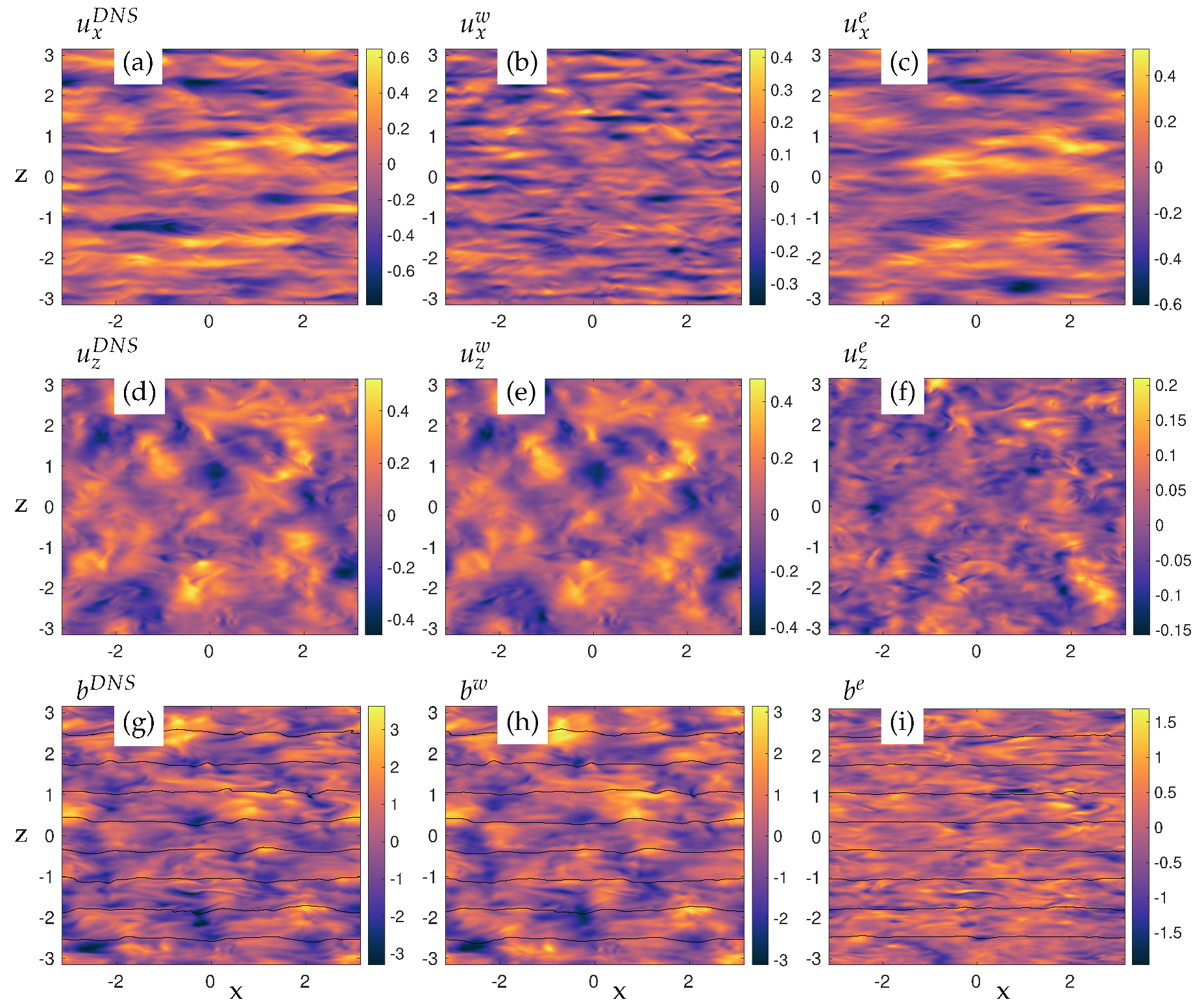
• Compute the 3D inverse Fourier transform in physical space, which permits recovering the wave and eddy fields in physical space and to visualize them.

Note that, in Step 3 of the filtering, the VSHF part of the horizontal velocity of the wave component with an angular frequency $\omega \simeq 0$ and with a horizontal wavenumber $k_h=0$ is removed. It does not appear either in the eddy component but it appears in the full velocity field. This is done because the VSHF would dominate the horizontal velocity field of the wave. Of course, this algorithm is computationally demanding in terms of both CPU time and memory storage.

4.2. Application to the Sweeping by Horizontal Velocity of Saint-Andrews cross Wave Propagation

In this section, the previous technique presented to separate the wave and the eddy components of the flow in Section 4.1 is applied on the same numerical simulation as in Section 3.1.2. The numerical parameters are also the same as in Section 3.1.2. Therefore, the chosen convective velocity is $\mathbf{c}=({10}^{-2},0,0)$. As the convective velocity is in only one direction, one could decide to refine the filtering in Step 3 of Section 4.1 to take only one direction into account. However, for simplicity, the filtering technique is kept as if the convective flow were in both positive and negative x direction. According to Step 3 of the method, we computed the vertical velocity $u_z(\mathbf{k},\omega )$ in four-dimensional space $(\mathbf{k},\omega )$. Since the 4D filtering is defined for every $(\mathbf{k},\omega )$, the velocity is either a wave part $u_z=u_z^w$ or an eddy part $u_z=u_z^e$, depending on the value of $(\mathbf{k},\omega )$. Then, the three vertical densities of the energy are defined (denoted with ⋆ to distinguish them with the previous energy given in Equation (5) and associated to $u_z$, $u_z^w$ and $u_z^e$:

$$\begin{array}{ccc}\hfill E_z^{\star }(\theta ,\omega )& =& \sum _{\theta \left(\mathbf{k}\right)\in I_{\theta },0\le \left|\mathbf{k}\right|\le k_{max}}\frac{1}{2}{\left|u_z(\mathbf{k},\omega )\right|}^2\hfill \end{array}$$

(17)

$$\begin{array}{ccc}\hfill E_z^{\star ,e,w}(\theta ,\omega )& =& \sum _{\theta \left(\mathbf{k}\right)\in I_{\theta },0\le \left|\mathbf{k}\right|\le k_{max}}\frac{1}{2}{\left|u_z^{e,w}(\mathbf{k},\omega )\right|}^2\hfill \end{array}$$

(18)

with this definition, $E_z^{\star }(\theta ,\omega )=E_z^{\star ,e}(\theta ,\omega )+E_z^{\star ,w}(\theta ,\omega )$. In Figure 9, one can see $E_z^{\star }$ for the full vertical velocity field (Figure 9a), the wave part $E_z^{\star ,w}$ (Figure 9b) and the eddy part $E_z^{\star ,e}$ (Figure 9c). In Figure 9c, we see that there is no energy along the dispersion relation (indicated with a red dashed line). This is the imprint of the discretization error of the filtering technique. Furthermore, the density of vertical energy is quite low in Figure 9c when, at the same location in ($\theta ,\omega$) plane in Figure 9b, the density of vertical energy is high. Indeed, most of the energy in this area comes from the waves that have been modified in angular frequency by the sweeping effect (for large wavenumber $k_x$, i.e., small scale). It is the manifestation of the density of energy sharing the same coordinate in the ($\theta$,$\omega$) plane, but for a different wavevector $\mathbf{k}$ and consequently a different sweeping effect.

Compared to the total energy in Figure 9b using the first separation method, our 4D analysis appears more precise—i.e., without vertical line—whereas no treatment such as Hann windowing is applied to the data. The main reason for this is due to the difference in the two algorithms for obtaining the energy density: The first algorithm gathers the flow component in a $\theta \in I_{\theta }$ domain before doing the time Fourier transform. It is only after applying the Fourier transform that the energy density is computed. To understand the link between the two methods, by analogy with the total energy defined previously in Equation (5), we define the vertical energy by:

$$\begin{array}{c}\hfill E_z(\theta ,\omega )=\frac{1}{2}{\left|\sum _{\theta \left(\mathbf{k}\right)\in I_{\theta },0\le \left|\mathbf{k}\right|\le k_{max}}\mathbf{u}(\mathbf{k},\omega )\right|}^2\end{array}$$

(19)

The second technique, which is more computationally expensive, starts with the time Fourier transform of the flow component, then summing them in the $\theta \in I_{\theta }$ domain and finally computing the energy density. As shown in [23], the difference between the two formulations of vertical density of energy is:

$$E_z(\theta ,\omega )=E_z^{\star }(\theta ,\omega )+\mathrm{Re}\left\{\sum _{\begin{array}{c}\theta \left(\mathbf{k}\right)\in I_{\theta }\\ \theta \left({\mathbf{k}}^{\prime }\right)\in I_{\theta }\\ {\mathbf{k}}^{\prime }\ne \mathbf{k}\end{array}}\mathbf{u}(\mathbf{k},\omega )\mathbf{u}({\mathbf{k}}^{\prime },\omega )\right\}$$

(20)

with ${\mathbf{k}}^{\prime }$ a different wavevector from $\mathbf{k}$ sharing the same domain $I_{\theta }$. The second term on the right-hand side corresponds to the error done by the first technique against the second one. The error corresponds to the crossing energy sharing the same domain $I_{\theta }$. This difference can be summed up in one sentence: the energy of the sum of the flow component in a domain $I_{\theta }$ is different from the sum of the energy of the flow component in the same domain $I_{\theta }$. The final result ends up being slightly different for laminar cases. For a turbulent case, we assume that the correlation term $<\mathbf{u}(\mathbf{k},t)\mathbf{u}({\mathbf{k}}^{\prime },t)>$ is almost zero on average.

After analysis in the domain $(\mathbf{k},\omega )$, we come back to physical space $(\mathbf{x},t)$, where the vertical velocity $u_z(\mathbf{x},t)$ is decomposed into wave and eddy parts $u_z(\mathbf{x},t)=u_z^e(\mathbf{x},t)+u_z^w(\mathbf{x},t)$. Figure 10 shows $u_z^e(\mathbf{x},t)$ and $u_z^w(\mathbf{x},t)$. In the eddy component (Figure 10b), only the Dirac in space is visible, whereas for the wave component (Figure 10a) only the wave propagation is visible. By comparing the sum of Figure 10a,b, the same kind of flow is obtained as in Figure 5a. Therefore, we can safely assume that, for the case of simple, laminar, convective flow, this filtering technique works rather well.

In the following, this analysis is applied to a DNS at moderately low Froude number and at low buoyancy Reynolds number.

4.3. DNS and Numerical Parameters

In contrast with the previous characterization of Section 3, in which we analyze the effect of large-scale mean field on the propagation of internal gravity waves produced by harmonic monochromatic forcing, and its trace on the statistics in spectral space, we consider here stratified turbulence obtained by Direct Numerical Simulations of the full nonlinear Navier–Stokes–Boussinesq equations. The corresponding field is then subjected to analysis by four-dimensional Fourier transform (FFT4D). As proposed by Maffioli [28], the flow is produced by forcing the momentum conservation equation, until statistical stationarity is reached. As presented in Section 2.2, the force ${\mathbf{F}}_u$ is applied at very large-scale in a cylindrical shell of radius $k_h=4$ and vertical extent $1\le k_v\le 3$, thus the forcing wavenumber is approximately $k_{forc}\simeq 5$ and the angles of forced wavevectors is in the range $0.24\mathrm{rad}<\left|\theta \right|<0.65\mathrm{rad}$. This means that the VSHF is not directly fed by the forcing, so that its growth is limited, even if it eventually becomes energetically dominant in the flow. The injected power is $P=<{\mathbf{F}}_u·\mathbf{u}>=0.01$. The resolution is $n_{grid}=256$ points in each direction, viscosity is $\nu =1/2500$, the Brunt–Väisälä frequency is $N=5$ and the time step is $\Delta t=0.005$.

The simulation is run until a statistically stationary state for total kinetic energy is reached. In this state, the Froude number is $\mathit{Fr}=\epsilon /N{u}_h^2=0.07$, where $\epsilon$ is the dissipation of kinetic energy and $u_h={(K_h-K_{shear})}^{1/2}$ is the rms of horizontal velocity component with $K_h$ the horizontal kinetic energy and $K_{shear}$ the shear mode energy (i.e., energy of all the $k_h=0$ Fourier modes). The Kolmogorov length scale is $\eta ={({\nu }^3/\epsilon )}^{0.25}=9\times {10}^{-3}$ and the Kolmogorov time scale is ${\tau }_{\eta }={(\nu /\epsilon )}^{0.5}=0.2$. The buoyancy Reynolds number is ${\mathit{Re}}_b=\epsilon /\nu N^2=1$. The integral length scale $L=0.4$ is rather large, resulting in a flow dominated by waves and explaining why the Taylor-length-scale-based Reynolds number is high as well ${\mathit{Re}}_{\lambda }=95$. The Ozmidov scale is $k_0={(N^3/\epsilon )}^{1/2}\approx 100\ge k_{max}$, so that wave motion is expected to be mixed with turbulent motion at all flow scales.

The five-step algorithm for spatiotemporal decomposition is applied on velocity and buoyancy using 1000 snapshots of these fields separated by a time step of $\Delta t^{\prime }=10\Delta t=0.05$. The total time span is therefore $T=39.8T_N$ where $T_N=2\pi /N$ is the Brunt–Väisälä period. Due to this discretization of frequency with a step $\Delta \omega =2\pi /T$, the angular frequency $\omega$ is determined to within $\Delta \omega$ accuracy, or equivalently the angular frequency cut-off is $\Delta \omega$. The filtered range described in Equation (16) is therefore also defined within a $2\Delta \omega$ accuracy.

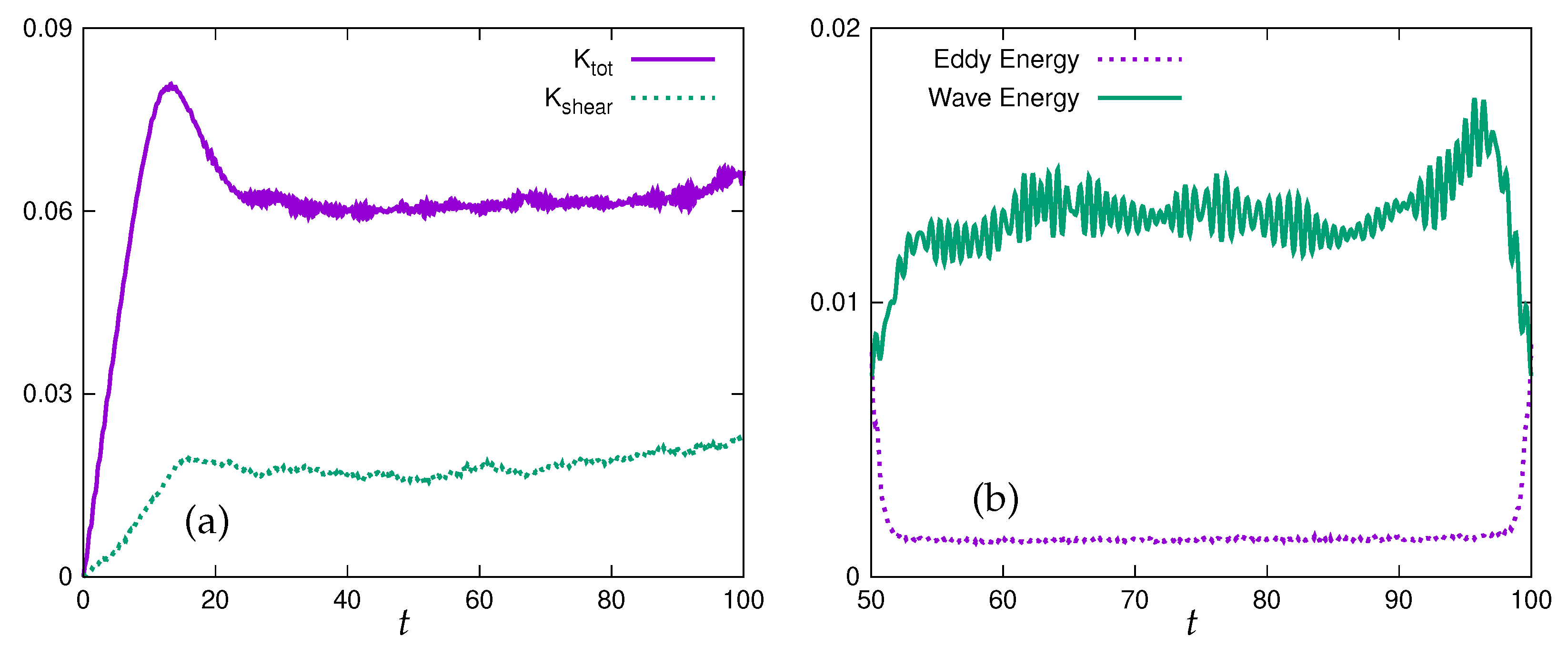
4.4. Estimation of the Sweeping Velocity

As explained in Section 3.3, the VSHF can sometimes dominate the overall structure of the flow. To check this in our numerical simulation, the kinetic energy of the VSHF flow $K_{shear}$ based on horizontal velocity ${\mathbf{u}}_{shear}=\mathbf{u}({\mathbf{k}}_h=0,k_z)$, and the total kinetic energy $K_{tot}$ are obtained as:

$$\begin{array}{cc}\hfill & K_{shear}\left(t\right)=0.5\sum _{k_z}\left(u_x^2({\mathbf{k}}_h=0,k_z,t)+u_y^2({\mathbf{k}}_h=0,k_z,t)\right)\end{array}$$

(21)

$$\begin{array}{c}{K}_{tot}\left(t\right)=0.5\sum _{k_x,k_y,k_z}\left(u_x^2(k_x,k_y,k_z,t)+u_y^2(k_x,k_y,k_z,t)+u_z^2(k_x,k_y,k_z,t)\right)\end{array}$$

(22)

Figure 11a shows the time evolution of $K_{shear}$ and $K_{tot}$ from the beginning of the simulation, where initial conditions with zero velocity and density fluctuations were used. The statistically steady state is reached at $t\simeq 30$, and there is a slow growth of energy at the end of the simulation, due to the growth of VSHF. The kinetic energy of the VSHF amounts to about a third of the total kinetic energy, so that the VSHF can be considered as the main source of modification of wave frequency by sweeping. To obtain the sweeping velocity related to the shear, one computes a rms shear velocity in the x and y directions $(u_{shear,x},u_{shear,y})$ from the shear kinetic energy $K_{shear}$:

$$\begin{array}{c}\hfill u_{shear,x}=u_{shear,y}=\sqrt{K_{shear}}\approx 0.14.\end{array}$$

(23)

Therefore, the sweeping velocity is estimated as $\mathbf{c}=(u_{shear,x},u_{shear,y},0)$ and in the numerical simulation, we use $\mathbf{c}=(0.14,0.14,0)$ from Equation (23). Choosing a different sweeping velocity would inevitably change the result of the filtering, so that the choice of the sweeping velocity is probably the main source of error of this technique. Here, we think that most of the sweeping effect comes from the VSHF mode, but this is suggestive.

4.5. Time-Windowing for the Time Fourier Transform

The choice of parameters for the time span over which Fourier transforms are done can be of importance, since a too narrow time-window or too sparse time points can lead to significant error in angular frequency estimates. Therefore, after transforming the velocity and buoyancy fields back to physical time t domain, we compute the time-evolution of the wave and the eddy contributions to vertical kinetic energy:

$$E_z^{\star ,e,w}\left(t\right)=\sum _{0\le \mathbf{k}\le k_{max}}\frac{1}{2}{\left|u_z^{e,w}(\mathbf{k},t)\right|}^2.$$

(24)

These energies are plotted in Figure 11b. We first observe that the energy in the wave part is about six times larger than the energy in the eddy part. Second, we see that for most of the time domain, away from the boundaries $t=50$ or $t=100$, the energies evolution only consists of fluctuations around a mean value. The appearance of edge zones in the evolution is due to the filtering technique which uses frequency-separated components that break up the periodic structure of the velocity field and result in a transition period at the edge of the time domain. However, these edge zones are limited in extent, so that we use no windowing technique such as Hann windowing, as often done in, e.g., experimental data processing. Furthermore, after a windowing technique, to recover the amplitude or the density of energy correctly, the signal needs to be modified by a different factor which might lead to inaccuracies later on in the energy spectrum and the visualization of the flow components. In the following, the presented statistics are obtained using only the part of the time window away from the edge zones.

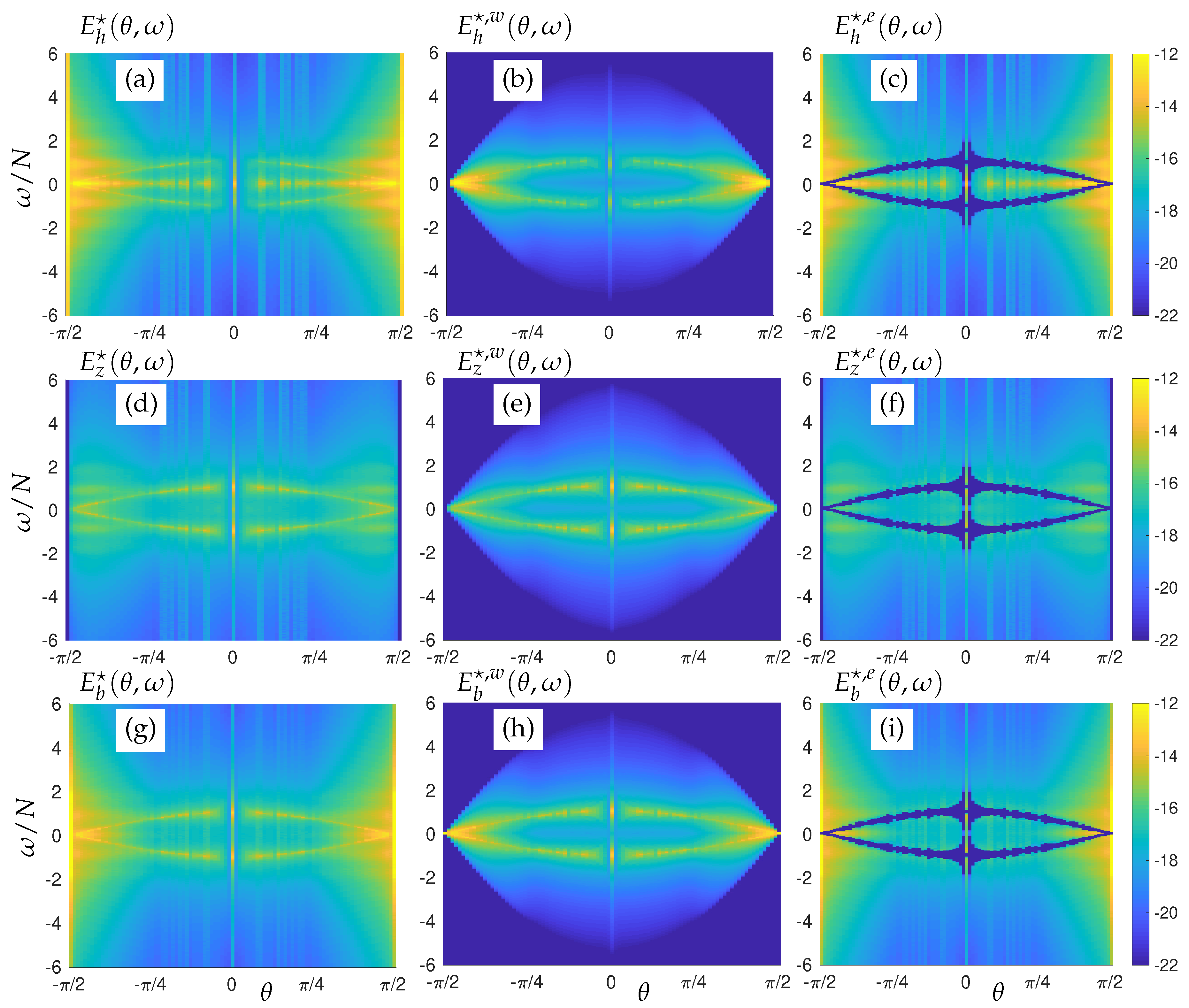
4.6. Energy Distribution in the $(\theta ,\omega )$ Plane

The filtering technique is applied on the four variables $f=u_x$, $u_y$, $u_z$, and b obtained from the DNS, by the five-step algorithm method explained in Section 4.1. The representation of the results requires a reduction of the amount of information contained in the 4D-fields depending on $(\mathbf{k},\omega )$. Therefore, the fields are averaged over wavenumber k and azimuthal angle $\phi$ to retain only the two dimensional dependence on ($\theta$, $\omega$). Thus, by analogy with the vertical density of energy defined in Equation (17), we define the averaged horizontal and potential energies by:

$$\begin{array}{ccc}\hfill E_h^{\star }(\theta ,\omega )& =& \sum _{\theta \left(\mathbf{k}\right)=\theta ,0\le \left|\mathbf{k}\right|\le k_{max}}\frac{1}{2}\left(|u_x{(\mathbf{k},\omega )|}^2+{\left|u_y(\mathbf{k},\omega )\right|}^2\right)\hfill \end{array}$$

(25)

$$\begin{array}{ccc}\hfill E_b^{\star }(\theta ,\omega )& =& \sum _{\theta \left(\mathbf{k}\right)=\theta ,0\le \left|\mathbf{k}\right|\le k_{max}}\frac{1}{2N^2}{\left|b(\mathbf{k},\omega )\right|}^2.\hfill \end{array}$$

(26)

These quantities are not the same as the energy density defined in Section 2.3. The 4D-transform technique is more expensive, but more accurate in terms of determination of the wave contents of the flow than the method of Section 2.3.

Figure 12 shows the results obtained when applying the 4D-decomposition technique to the results of our simulation. Figure 12 first column show the distributions of horizontal, vertical and potential energies in the $(\theta ,\omega )$ plane. Figure 12 (Column 2) shows the distributions of their wave contents as obtained after the separating procedure and Figure 12 (Column 3) shows the distribution of the eddy contents of the same energies.

Figure 12 (Column 1)—for the complete horizontal, vertical and buoyancy energies $E_h^{\star }$, $E_z^{\star }$ and $E_b^{\star }$—shows that, after the spatiotemporal decomposition, the energy is concentrated on the dispersion relation curve of the waves, as well as away from the dispersion relation, for high angle $\theta$ and for a large range of angular frequency $\omega$. We observe a concentration of horizontal and buoyancy energies along wavevectors $\mathbf{k}$s almost vertical ($\theta$ close to $\pm \pi /2$), which can be attributed to horizontal structures. In addition, Figure 12a exhibits a concentration of horizontal energy density along the line $\omega \simeq 0$, which indicates motion unrelated to the waves, thus could be attributed to the eddy contents of the flow. The structure of horizontally-stretched pancake-like eddies comes to mind, as observed in previous studies (e.g., the experimental study by Fincham et al. [37]).

Similar to the definitions in Equations (17), (25) and (26) of horizontal and vertical kinetic energies and of potential energy, we define the same energies for the wave and eddy contents of the flow by using the analogy with vertical density of energy Equation (18):

• For horizontal and potential energy density, we define the wave part of the energies, respectively noted $E_h^{\star ,w}(\theta ,\omega )$, $E_b^{\star ,w}(\theta ,\omega )$, based on $u_x^w$,$u_y^w$, and $b^w$.
• Similarly, we define the eddy part of energy, with energies noted $E_h^{\star ,e}(\theta ,\omega )$, $E_b^{\star ,e}(\theta ,\omega )$, based on $u_x^e$, $u_y^e$, $b^e$.

These quantities are plotted in Figure 12 (Columns 2 and 3). By comparing the wave part (${*}^w$) and eddy part (${*}^e$), our decomposition separates clearly the wave energy, corresponding to the condensation of the energy around the dispersion relation curve (Figure 12, Column 2), from the energy associated to more general turbulent motion. This other motion is either the eddy part of the flow, with a concentration of energy around $\omega \simeq 0$ in Figure 12c, or horizontal structure which concentrates energy along vertical wave number regions (Figure 12c,i). The energy of the waves appears to be concentrated around the forcing angle $0.24\mathrm{rad}<\left|\theta \right|<0.65\mathrm{rad}$, and decreases only for $E_z^{\star ,w}(\theta ,\omega )$ where $\theta \simeq \pm \pi /2$. The overall energy density level in Figure 12f is clearly lower than that of the other figures, since it corresponds to the vertical kinetic energy of the non-wavy and non-VSHF part of the flow.

Moreover, some energy appears in the neighborhood of the relation dispersion curve (light blue part in Figure 12, Column 2) probably due to wave numbers that undergo a strong sweeping effect due to their small scale. For example, the relative sweeping amplitude is larger for a close-to-horizontal wavevector with large wavenumber—such that $k_x\gg k_z\gg 1$ so that $\theta \simeq 0$—than for a wavevector at smaller wavenumber such that $k_x\sim 1\gg k_z\sim 0$ for which $\theta \simeq 0$. The strong sweeping effect can also be seen in Figure 12 (Column 3) where the edge of the density of energy along the dispersion relation is irregular. Indeed, at some angle $\theta$, a small value of $k_x\sim 0$ and $k_y\sim 0$ might not exist in the spectral discretization, therefore resulting in a minimum sweeping effect already large as it is multiplied by a large value ($c_x=c_y=0.14$). For another angle $\theta$, there might exist smaller values of $k_x$ and $k_y$, which result in a minimum sweeping effect smaller as well. This effect does not exist in Figure 9b because the sweeping velocity is small $\mathbf{c}=({10}^{-2},0,0)$.

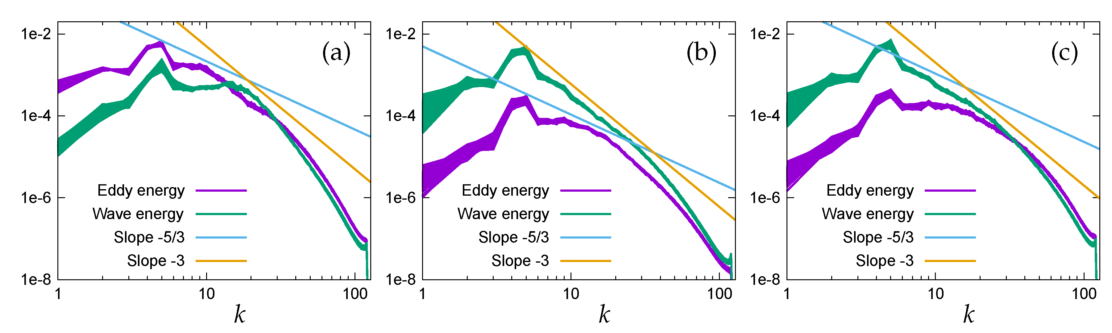
4.7. Energy Spectra

The wave-eddy decomposition proposed above can be used to obtain several statistics of different nature for the separate wave and eddy contents.

We focus here on the energy spectrum at scale k for the wave and eddy parts, which can be computed for horizontal, vertical and potential energies, respectively, as

$$\begin{array}{ccc}\hfill E_h^{\star ,e,w}(k,t)& =& \sum _{\left|\mathbf{k}\right|=k}\frac{1}{2}\left(|u_x^{e,w}{(\mathbf{k},t)|}^2+{\left|u_y^{e,w}(\mathbf{k},t)\right|}^2\right)\hfill \end{array}$$

(27)

$$\begin{array}{ccc}\hfill E_z^{\star ,e,w}(k,t)& =& \sum _{\left|\mathbf{k}\right|=k}\frac{1}{2}{\left|u_z^{e,w}(\mathbf{k},t)\right|}^2\hfill \end{array}$$

(28)

$$\begin{array}{ccc}\hfill E_b^{\star ,e,w}(k,t)& =& \sum _{\left|\mathbf{k}\right|=k}\frac{1}{2N^2}{\left|b^{e,w}(\mathbf{k},t)\right|}^2\hfill \end{array}$$

(29)

The energy spectra are plotted in Figure 13. At large-scale, the eddy part is dominant for horizontal energy (Figure 13a), whereas the wave part is dominant for both vertical (Figure 13b) and potential energies (Figure 13c). This is consistent with results in the previous section, wherein the accumulation of energy density along the dispersion relation curve is more important in vertical and potential energy, whereas the neighborhood of frequency $\omega \sim 0$ accumulates more eddy energy. However, at smaller scales, there seems to be an equipartition of eddy and wave energy in the horizontal energy spectrum and the buoyancy energy spectrum. Moreover, Figure 13b for the vertical kinetic energy spectrum shows that wave energy is dominant even at small scales.

Since the Reynolds number of our simulation is relatively low, one cannot expect to observe clear inertial scalings. We note however that the wave and eddy energy spectra seem to exhibit scalings respectively close to $k^{-3}$ and $k^{-5/3}$ for both the horizontal and the vertical kinetic energy spectra. Nonetheless, this is still suggestive and more remains to be done to understand what the correct scaling should be.

Finally, Figure 13 shows several spectra in the time interval $t\in [50;100]$, where the flow is statistically steady in terms of total integrated kinetic energy. It is not possible to distinguish between the different curves because they are on top of each other, but by looking at the width of each line, one can understand how much the energy spectra change through time. The different curves for each kind of spectrum show that there is some variability in the spectra with time, especially in the largest scale in the infrared spectrum range. However, the spectra are still remarkably stable on average over the chosen period.

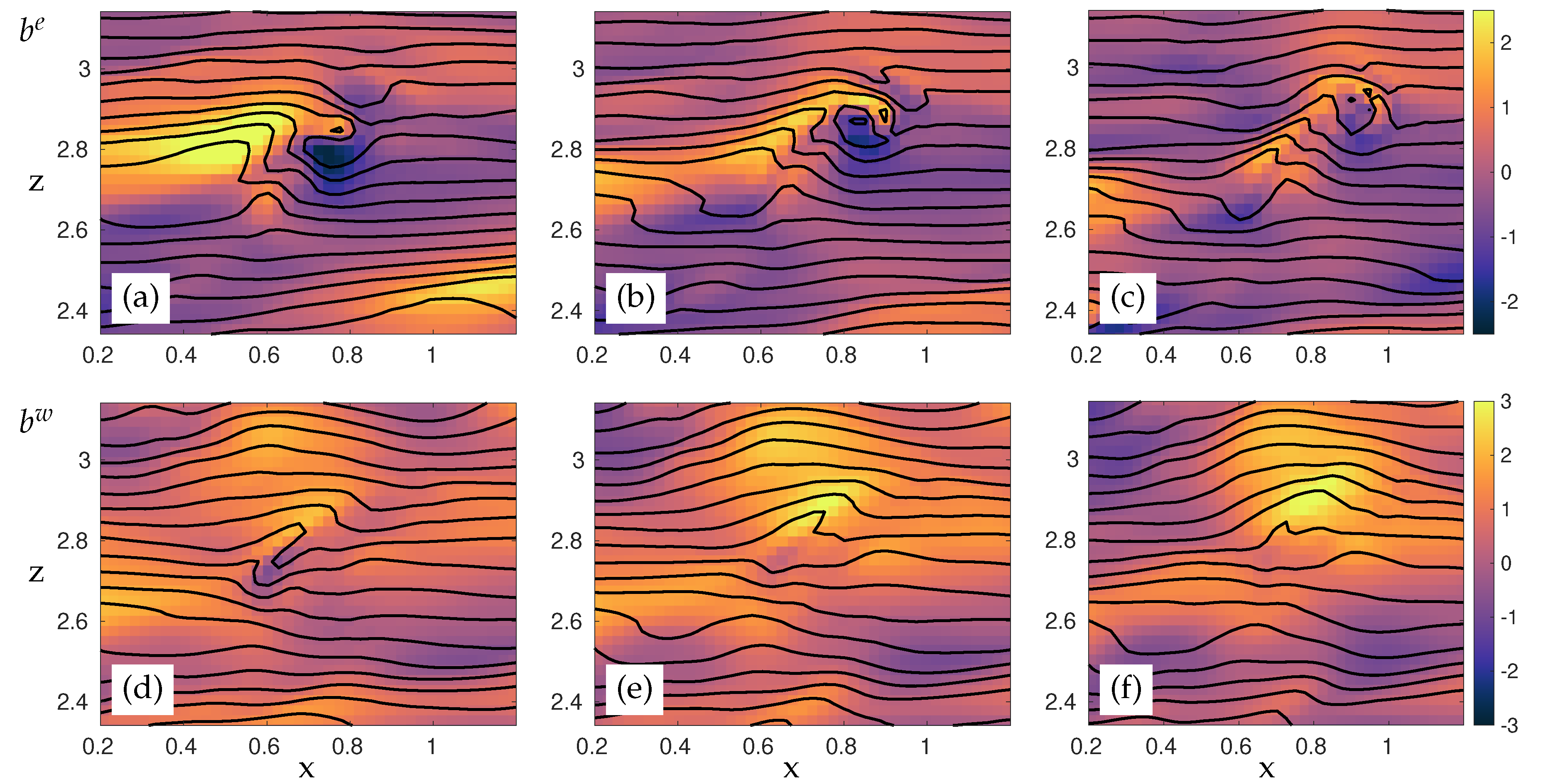
4.8. Physical Space Distribution of Wave and Eddy Fields

The final use of our decomposition for the current DNS results is the physical space distribution of the field. Upon computing the 3D spatial inverse Fourier transform of the separated wave and eddy spectral coefficients, one obtains the velocity and buoyancy fields $u_x^{DNS}$$,u_y^{DNS}$, $u_z^{DNS}$, and $b^{DNS}$ decomposed in terms of their wave and eddy parts $u_x^{e,w}$, $u_y^{e,w}$, $u_z^{e,w}$, and $b^{e,w}$ in physical space. Figure 14, shows their distribution in the vertical (x,z) plane at mid y-span. Therefore, the wave and eddy parts of the velocity field and of the buoyancy field are recovered. In the first column of Figure 14, the full field is plotted as for classical 3D DNS results. In the second column of Figure 14, the distribution of the wave contents of the velocity field is represented, and, in the third column of Figure 14, that of the eddy part is shown. The time evolution of these fields is informative of their proper kinematics. Therefore, the animation of these three decompositions for the three variables in the time interval $t\in [60;90]$ is available in the Supplementary Materials (see Videoa S1–S3). We recall that the shear mode is not taken into account either in the wave part or in the vortex part.

In Figure 14 (Rows 2 and 3), we represent the vertical velocity field $u_z(x,z)$ and buoyancy field b in $(x,z)$ plane and decomposed into a wave and an eddy parts. It appears that the wave part is at a bigger scale than the eddy part of these two fields. This underlines that, in the Energy spectrum of Figure 13b,c, the wave energy dominates the eddy energy at larger scale. In addition, their time evolution shows that the wave part of $u_z(x,z)$ and b oscillates like a wave while it is not the case in the eddy part (Videos S2 and S3). On the other hand, the decomposition of the horizontal velocity $u_x(x,z)$, which is illustrated in Figure 14 (Row 1), shows clearly the overall horizontal layering either for wave and eddy parts. These layers seem to be at a smaller vertical scale for the wave part than for the eddy part of the $u_x$ field.

These observations match with the Energy spectrum of Figure 13a, wherein the eddy energy dominates the wave energy at large scale. Again, the time evolution shows that the wave part of $u_x(x,z)$ oscillates as a wave while it is not the case in the eddy part. The layers in the wave part $u_x^w$ appear surprising, even though, intuitively, the layering is associated with the eddy part $u_x^e$. Indeed, $u_z^w$ contains only the vertical component of the poloidal part of velocity (see Appendix B and Figure A2) which is associated to linear wave, whereas $u_x^w$ contains a mix of horizontal components of the poloidal and toroidal part of the velocity, which are associated with the linear wave and the horizontal vortex respectively (see Appendix B and Figure A2). The direct analysis on the horizontal velocity appears as a limitation of our method because we call wave part $u_1^w$ any mode of $u_1$ which has a frequency and a wavevector included in the dispersion relation without distinguishing the poloidal and toroidal parts in $u_x$. It would be preferable to use our method directly on the poloidal and toroidal components separately. This limitation occurs in experimental work where the evolution of a three-dimensional field is generally not possible.

From a qualitative point of view, this new decomposition should work when the domain of the waves and the domain of the eddies are disjoint in ($\mathbf{k},\omega$) space. One expects the angular frequency of the eddies to be small (i.e., $\omega \simeq 0$, see Figure 13c) whereas the angular frequency of the waves are engulfed between the positive and negative sweeping effect (${\omega }_r-|\mathbf{c}·\mathbf{k}|<\omega <{\omega }_r+|\mathbf{c}·\mathbf{k}|$). Therefore, if the sweeping effect due to the advective velocity c is strong enough, then some waves with high amplitude of wavevector have a strong deviation of frequency by the sweeping effect reaching a zero frequency ($\omega =Ncos\theta +\mathbf{c}·\mathbf{k}\simeq 0$) and therefore sharing the same frequency as the majority of the eddies. This happens for the higher wave number $k_{\eta }=1/\eta$ based on the Kolmogorov scale $\eta$. From this observation, one could compute a dimensionless number: the ratio of the Brunt–Väisälä frequency N over the sweeping effect $k_{\eta }c$: $N/\left(k_{\eta }c\right)$. If this ratio is higher than one, the domains of the waves and eddies are well separated in ($\mathbf{k},\omega$) space: $\omega \simeq 0$ for the eddies and $\omega >0$ for the waves. If the ratio is lower than one, the domains of the waves and eddies overlap in ($\mathbf{k},\omega$) space. In this study, this dimensionless number would be close to $0.2$ with $c\simeq 0.2$, $N=5$ and $k_{\eta }\simeq 110$. This might explain why the approximation of the horizontal wave component is only approximative, as most of the horizontal energy comes from the motion of the eddies. The ratio $N/\left(k_{\eta }c\right)\ge 1$ could be obtained by changing N or decreasing c for the same resolution.

Nevertheless, apart from these limitations on the horizontal velocity field, the analysis of vertical velocity field $u_z(x,z)$ and buoyancy field b provide valuable information about the overturn of density. We recall that in the standard wave–vortex decomposition [17] all the buoyancy field b is attributed to wave motion. This is not the case with the method we propose, and we can classify the density turnover in the eddy part. We illustrate this distinction in Figure 15 with a zoom in of the temporal evolution of the buoyancy field in the vertical $(x,z)$ plane, for one overturning event. We observe that the eddy part of b (Figure 15 first line) shows an overturn of density [38] by looking at the black iso-density lines: when the iso-density lines are on top of one another (as in Figure 15b), heavy fluid is on top of lighter fluid. Consequently, mixing is occurring as heavier fluid tends to flow below lighter fluid. On the contrary, in Figure 15 (Row 2), which corresponds to the wave part of the buoyancy field, no similar topological arrangement is seen. However, the amplitude of iso-density lines in the middle of Figure 15d is quite high, whereas, in Figure 15e,f, it is lower. This could suggest that the waves are interacting and are breaking into eddies, but this is still speculative. Other events of this type are visible in the animation and no density overturn is visible on the wave part of b. Nonetheless, this shows that the present wave-eddy decomposition successfully separates a turbulent event, the overturning of density, from the wave component.

By performing this decomposition in physical space, it is then possible to extend the analysis to other statistics in physical space (structure function, two-point correlation, etc.) on each part separately in order to obtain information on the role of each part and their interaction.

5. Conclusions and Perspectives

In this work, we propose numerical simulations of Navier–Stokes–Boussinesq for stably stratified flows generated by specific forcings, in which we use two spatiotemporal techniques for separating the wave motion from the eddy motion. The statistical characterization is mostly based on the computation of the energy density in the $(\theta ,\omega )$ plane.

The first part presents a spatiotemporal analysis used in simple laminar cases (homogeneous advective flow and shear flow) in order to quantify the modification by a large-scale mean flow of the propagation of the waves, in terms of wave frequency and the observed dispersion relation in the simulations. It appears that the main physical reason for the modification of the wave frequency is the sweeping effect. This effect corresponds to the advection of the wave packets by a large-scale flow, in particular by vertically sheared horizontal flow (VSHF).

The second part presents a new spatiotemporal decomposition, more precise but more numerically expensive than the first method: the partitioning of waves and eddies is done by separating the angular frequency of the waves from the rest of the turbulence. This separation takes into account the sweeping effect due to the shear part of the flow (VSHF), which is supposed to consist of a large-scale advecting velocity. From this separation, energy statistics and visualization of the velocity and buoyancy field can be done for the wave and the eddy parts of the flow.

Such a decomposition is more sophisticated than the decomposition proposed by Riley [17] in the physical space only. The latter decomposition is solely based on the physical domain and lacks the temporal dependence of the wave component to be fully effective. Therefore, the spatiotemporal technique proposed here could be more effective, especially if it is applied in complement to the spatial decomposition proposed by Riley. From there, it is possible to use advanced statistical characterization in physical space (structure function, two-point correlation, etc.) to obtain further information on the role of the different parts and their interaction. For example, our decomposition is able to distinguish a turnover of the density field associated with the eddy part from an oscillation of the density field associated with the wave part. However, it still needs to be further studied. In our present work, observations of the sweeping effect done on laminar cases are extended to the turbulent case. However, the analogy between the turbulent and laminar cases may be limited. A better understanding of the sweeping effect would therefore be needed for turbulent cases. The other main limitation of this decomposition is its dependency on the choice of the advective velocity responsible for the sweeping effect. We assume that the VSHF is the main source of sweeping effect, which seems to be a good approximation but not a completely universal one. As the result of the decomposition depends significantly on the chosen advective velocity, a better evaluation of this velocity is of importance for the accuracy of our decomposition. This technique is valid when the domain of the waves and the domain of the eddies are well separated in ($\mathbf{k},\omega$) space. To quantify this separation, a dimensionless number has been introduced in Section 4.8, the ratio of the Brunt–Väisälä frequency N over the sweeping effect $k_{\eta }c$: $N/\left(k_{\eta }c\right)$. Even though $N/\left(k_{\eta }c\right)\simeq 0.2$ in this study, which means that the sweeping effect is strong against the stratification, waves and eddies have been well separated for the buoyancy and vertical velocity field. Therefore, further work remains to be done to understand what the limits of this new algorithm are against the dimensionless number $N/\left(k_{\eta }c\right)$.

We have shown the applicability of our method on an instance of turbulence where the wave regime dominates the eddy regime, at large Ozmidov scale and $R{e}_b\simeq 1$. It will be necessary to extend our decomposition to a wide range of parameters in terms of Froude number (lower $Fr$) and buoyancy Reynolds number (higher $R{e}_b$). It will also be necessary to increase the Ozmidov scale and retaining enough wave contents. For this, numerical simulations are required where both waves and eddies dominate a different domain of the energy spectrum, but they would also be more computationally expensive.

If this new decomposition was successfully further developed, many new physical applications could be proposed: computing the ratio of energy between waves and eddies, or the different energy spectra against horizontal and vertical wavenumber. Another possibility would be to compute energy transfers between waves, eddies and themselves using similar techniques done in the case of magnetohydrodynamics [39]. Moreover, this spatiotemporal decomposition method could be applied to simulations of rotating turbulence for which experimental studies have already used a similar 4D Fourier technique [8], but more interestingly to mixed inertio-gravity waves in rotating and stably stratified flows.

References

- Pedlosky, J. Geophysical Fluid Dynamics; Springer: Berlin/Heidelberg, Germany, 1982. [Google Scholar]
- MacKinnon, J. Oceanography: Mountain waves in the deep ocean. Nature 2013, 501, 321. [Google Scholar] [CrossRef] [PubMed]
- MacKinnon, J.A.; Zhao, Z.; Whalen, C.B.; Waterhouse, A.F.; Trossman, D.S.; Sun, O.M.; St. Laurent, L.C.; Simmons, H.L.; Polzin, K.; Pinkel, R.; et al. Climate Process Team on Internal Wave-Driven Ocean Mixing. Bull. Am. Meteorol. Soc. 2017, 98, 2429–2454. [Google Scholar] [CrossRef] [PubMed]
- Bretherton, F.P. Momentum transport by gravity waves. Q. J. R. Meteorol. Soc. 1969, 95, 213–243. [Google Scholar] [CrossRef]
- Lighthill, M.J. Waves in Fluids; Cambridge University Press: Cambridge, UK, 2003. [Google Scholar]
- Nazarenko, S. Wave Turbulence; Springer: Berlin/Heidelberg, Germany, 2011; Volume 825. [Google Scholar]
- Dyachenko, A.; Lvov, Y.; Zakharov, V.E. Five-wave interaction on the surface of deep fluid. Phys. D Nonlinear Phenom. 1995, 87, 233–261. [Google Scholar] [CrossRef]
- Yarom, E.; Sharon, E. Experimental observation of steady inertial wave turbulence in deep rotating flows. Nat. Phys. 2014, 10, 510–514. [Google Scholar] [CrossRef]
- Le Reun, T.; Favier, B.; Barker, A.J.; Le Bars, M. Inertial Wave Turbulence Driven by Elliptical Instability. Phys. Rev. Lett. 2017, 119. [Google Scholar] [CrossRef]
- Clark di Leoni, P.; Mininni, P.D. Absorption of waves by large-scale winds in stratified turbulence. Phys. Rev. E 2015, 91. [Google Scholar] [CrossRef]
- Davidson, P.A.; Staplehurst, P.J.; Dalziel, S.B. On the evolution of eddies in a rapidly rotating system. J. Fluid Mech. 2006, 557, 135. [Google Scholar] [CrossRef]
- Fitzgerald, J.G.; Farrell, B.F. Statistical state dynamics of vertically sheared horizontal flows in two-dimensional stratified turbulence. J. Fluid Mech. 2018, 854, 544–590. [Google Scholar] [CrossRef]
- Alford, M.H.; MacKinnon, J.A.; Pinkel, R.; Klymak, J.M. Space–Time Scales of Shear in the North Pacific. J. Phys. Oceanogr. 2017, 47, 2455–2478. [Google Scholar] [CrossRef]
- Grimshaw, R. Nonlinear Internal Gravity Waves and Their Interaction with the Mean Wind. J. Atmos. Sci. 1975, 32, 1779–1793. [Google Scholar] [CrossRef]
- Gerkema, T.; Maas, L.R.M.; van Haren, H. A Note on the Role of Mean Flows in Doppler-Shifted Frequencies. J. Phys. Oceanogr. 2013, 43, 432–441. [Google Scholar] [CrossRef]
- Pinkel, R. Vortical and Internal Wave Shear and Strain. J. Phys. Oceanogr. 2014, 44, 2070–2092. [Google Scholar] [CrossRef]
- Riley, J.J.; Metcalfe, R.W.; Weissman, M.A. Direct numerical simulations of homogeneous turbulence in density-stratified fluids. AIP Conf. Proc. 1981, 76, 79–112. [Google Scholar] [CrossRef]
- Gibson, C.H. Internal waves, fossil turbulence, and composite ocean microstructure spectra. J. Fluid Mech. 1986, 168, 89–117. [Google Scholar] [CrossRef]
- Staquet, C.; Riley, J.J. On the velocity field associated with potential vorticity. Dyn. Atmos. Oceans 1989, 14, 93–123. [Google Scholar] [CrossRef]
- Sagaut, P.; Cambon, C. Homogeneous Turbulence Dynamics; Springer: Berlin/Heidelberg, Germany, 2008; Volume 10. [Google Scholar]
- Godeferd, F.S.; Cambon, C. Detailed investigation of energy transfers in homogeneous stratified turbulence. Phys. Fluids 1994, 6, 2084–2100. [Google Scholar] [CrossRef]
- Herbert, C.; Marino, R.; Rosenberg, D.; Pouquet, A. Waves and vortices in the inverse cascade regime of stratified turbulence with or without rotation. J. Fluid Mech. 2016, 806, 165–204. [Google Scholar] [CrossRef][Green Version]
- Maffioli, A.; Delache, A.; Godeferd, F. Signature and energetics of internal gravity waves in stratified turbulence. Phys. Rev. Fluids 2020, 2, 104802, submitted. [Google Scholar] [CrossRef]
- Pedlosky, J. Waves in the Ocean and Atmosphere: Introduction to Wave Dynamics; Springer: Berlin/Heidelberg, Germany, 2013. [Google Scholar]
- Rogallo, R.S. Numerical Experiments in Homogeneous Turbulence; National Aeronautics and Space Administration: Washington, DC, USA, 1981; Volume 81315.
- Pekurovsky, D. P3DFFT: A framework for parallel computations of Fourier transforms in three dimensions. SIAM J. Sci. Comput. 2012, 34, C192–C209. [Google Scholar] [CrossRef]
- Canuto, C.; Hussaini, M.Y.; Quarteroni, A.; Thomas, A., Jr. Spectral Methods in Fluid Dynamics; Springer: Berlin/Heidelberg, Germany, 2012. [Google Scholar]
- Maffioli, A. Vertical spectra of stratified turbulence at large horizontal scales. Phys. Rev. Fluids 2017, 2. [Google Scholar] [CrossRef]
- Campagne, A.; Gallet, B.; Moisy, F.; Cortet, P.P. Disentangling inertial waves from eddy turbulence in a forced rotating-turbulence experiment. Phys. Rev. E 2015, 91, 043016. [Google Scholar] [CrossRef] [PubMed]
- Smith, L.M.; Waleffe, F. Generation of slow large scales in forced rotating stratified turbulence. J. Fluid Mech. 2002, 451, 145–168. [Google Scholar] [CrossRef]
- Herring, J.R.; Métais, O. Numerical experiments in forced stably stratified turbulence. J. Fluid Mech. 1989, 202, 97–115. [Google Scholar] [CrossRef]
- Smith, L.M. Numerical study of two-dimensional stratified turbulence. Contemp. Math. 2001, 283, 91–106. [Google Scholar]
- Godeferd, F.S.; Staquet, C. Statistical modelling and direct numerical simulations of decaying stably stratified turbulence. Part 2. Large-scale and small-scale anisotropy. J. Fluid Mech. 2003, 486, 115–159. [Google Scholar] [CrossRef]
- Kumar, A.; Verma, M.K.; Sukhatme, J. Phenomenology of two-dimensional stably stratified turbulence under large-scale forcing. J. Turbul. 2017, 18, 219–239. [Google Scholar] [CrossRef]
- Ascani, F.; Firing, E.; McCreary, J.P.; Brandt, P.; Greatbatch, R.J. The deep equatorial ocean circulation in wind-forced numerical solutions. J. Phys. Oceanogr. 2015, 45, 1709–1734. [Google Scholar] [CrossRef]
- Galmiche, M.; Hunt, J. The formation of shear and density layers in stably stratified turbulent flows: Linear processes. J. Fluid Mech. 2002, 455, 243–262. [Google Scholar] [CrossRef]
- Fincham, A.M.; Maxworthy, T.; Spedding, G.R. Energy dissipation and vortex structurein freely decaying stratified grid turbulence. Dyn. Atmos. Oceans 1996, 23, 155–169. [Google Scholar] [CrossRef]
- Yakovenko, S.N. Development of instability and turbulence in overturning lee waves: The map of different scenarios in Re–Pr space. J. Phys. Conf. Ser. 2016, 722, 012048. [Google Scholar] [CrossRef]
- Alexakis, A.; Mininni, P.D.; Pouquet, A. Shell-to-shell energy transfer in magnetohydrodynamics. I. Steady state turbulence. Phys. Rev. E 2005, 72. [Google Scholar] [CrossRef] [PubMed]
- Herring, J.R. Approach of axisymmetric turbulence to isotropy. Phys. Fluids 1974, 17, 859–872. [Google Scholar] [CrossRef]