Morphology of the Wavenumber 1 and Wavenumber 2 Stratospheric Kelvin Waves Using the Long-Term Era-Interim Reanalysis Dataset

Abstract

The atmospheric Kelvin wave has been widely studied due to its importance in atmospheric dynamics. Since a long-term climatological study is absent in the literature, we have employed the two-dimensional fast Fourier transform (2D-FFT) method for the 40-year long-term reanalysis of the dataset, ERA-Interim, to investigate the properties of Kelvin waves with wavenumbers 1 (E1) and 2 (E2) at 6–24 days wave periods over the equatorial region of ±10° latitude between a 15 and 45 km altitude during the period 1979–2019. The spatio-temporal variations of the E1 and E2 wave amplitudes were compared to the information of stratospheric quasi-biennial oscillation (QBO), and the wave amplitudes were found to have an inter-QBO cycle variation that was related to sea surface temperature and convections, as well as an intra-QBO cycle variation that was caused by interactions between the waves and stratospheric mean flows. Also, the E1 waves with 6–10 day periods and the E2 waves with 6 days period were observed to penetrate the westerly regime of QBO, which has a thickness less than the vertical wavelengths of those waves, and the waves could further propagate upward to higher altitudes. In a case study of the period 2006–2013, the wave amplitudes showed a good correlation with the Niño 3.4 index, outgoing longwave radiation (OLR), and precipitation during 2006–2013, though this was not the case for the full time series. The present paper is the first report on the 40-year climatology of Kelvin waves, and the morphology of Kelvin waves will help us diagnose the anomalies of wave activity and QBO in the future.

1. Introduction

Atmospheric Kelvin waves are a branch of gravity waves with a horizontal wavelength on the planetary scale, and they propagate eastward and upward over equatorial (±10°) latitudes. These waves are equatorially trapped because of the Coriolis force. The wave amplitude peaks at the equator and exponentially decays with increasing latitudes [1].

Kelvin waves can be detected as perturbations in the atmospheric wind field, temperature, and pressure. In the 1960s, Matsuno [2], Holton, and Lindzen [3] predicted the existence of Kelvin waves using theoretical derivation, and soon Wallace and Kousky [4] discovered the existence of Kelvin waves from radiosonde observations. Since then, the properties of Kelvin waves have been investigated using radiosondes, rockets, radars, satellites, and model simulations [5,6,7,8,9,10,11,12,13,14,15]. A brief summary of the properties of Kelvin waves from the literature can be found in Table 1 in [16].

Based on wave period, Kelvin waves are further classified into three categories of slow (10–20 days), fast (6–10 days), and ultra-fast (2–5 days) Kelvin waves [4,8,13]. These waves have a variety of properties. The phase speed varies from 20–40 (slow), to 50–80 (fast), to faster than 100 (ultra-fast) m/s. The vertical wavelength also changes from 10 (slow), to 20 (fast), to 40 (ultra-fast) km. Slow Kelvin waves mainly exist in the lower stratosphere. Contrastingly, fast Kelvin waves have mainly appeared in the upper stratosphere and mesosphere. Different from the previous two categories, ultra-fast Kelvin waves not only appear in the stratosphere and mesosphere, but also can propagate into the lower thermosphere, and thus further affect the ionosphere in the variability of vertical drift and generation of irregularities [17,18,19].

Kelvin waves play a crucial role in atmospheric dynamics because they transfer the eastward momentum and energy from the troposphere into the stratosphere and even higher altitudes. Kelvin waves contribute about 30–50% of the magnitude of the wind reversal regarding the quasi-biennial oscillation (QBO), as well as 20–35% of the magnitude of the total wave forcing at 20–40 km [20].

Tropospheric convection is believed to be the source of the generation of Kelvin waves [21,22]. The waves excited by the slowly accumulated heating that evolves over the seasonal time scale are called the convective couple mode. These waves have a period of 5–10 days, a zonal wavenumber of 3–6, and a phase speed of 15 m/s [23,24]. On the other hand, there are also free mode Kelvin waves, which result from high-frequency convective heating releases (usually in days to weeks), and do not propagate coherently with the convective centers in the middle troposphere. These waves have a period of 10–20 days, a zonal wavenumber of 1 or 2, and a phase speed of 20–30 m/s [4,16].

Recently, Das and Pan [7] used the Kelvin wave amplitude extracted from the FORMOSAT-3/COSMIC mission, and the Niño 3.4 index (also known as oceanic Niño index, ONI), which is a kind of sea surface temperature (SST) anomaly index in the Niño 3.4 region (5° N–5° S, 120°–170° W), to investigate a fast descending event of the QBO westerly regime during the El Niño episode of 2009–2010. They reported significant enhancements of Kelvin wave amplitude during the El Niño episode, and concluded that the enhanced Kelvin waves may be produced by the processes (e.g., westerly wind events) generating the El Niño. Those enhanced waves further resulted in the fast descending event of the westerly QBO wind during the same epoch. Their study has faithfully demonstrated the relationship between the ocean, tropospheric convections, stratospheric waves, and winds.

Scientists have studied Kelvin waves for many decades. However, most studies focused on Kelvin waves with wavenumber 1 (we abbreviated it to “E1” in the present study, which means eastward propagating waves with wavenumber one) since they are dominant in amplitude. On the other hand, the Kelvin waves with wavenumber 2 (E2) have received less attention, even though they are the second significant component in amplitude. Therefore, we investigated both the E1 and E2 Kelvin waves in this study. Through knowledge of the waves, we can further understand atmospheric dynamics and energy balances as well as climate evolution, which may improve the weather forecast model. This investigation is confined to the stratospheric altitudes of 15–45 km, and we have further divided the stratosphere into three altitudinal ranges of the lower (15–25 km), middle (25–35 km), and upper (35–45 km) stratosphere. For Kelvin waves, especially the ultra-fast waves in the upper stratosphere, the mesosphere, and the lower thermosphere, one may refer to the recent paper [6]. In the present study, we used the wave properties and the “zonal mean zonal wind” (we abbreviated it to zonal wind in this paper) pattern from the ERA-Interim long-term (40 years) reanalysis data provided by the European Centre for Medium-Range Weather Forecasts (ECMWF). We reported the morphology of the E1 and E2 waves in the stratosphere through the wave spectra and spatio-temporal distributions of the wave amplitudes. Besides this, we also studied the correlation between the waves and zonal wind as well as tropospheric convections in the present study.

Please note that in this paper, we used (reserved) the word “period” for describing “wave period”. On the other hand, we used “epoch” and “duration” to describe the time of some phenomena or events, though those words are not the customary ones people use to describe the “time period”. We also use the words “faster” and “slower” to group the waves at different periods, as this helped us to avoid using wordy descriptions. The adjectives faster/slower mean the wave(s) has a shorter/longer period compared to another one(s), though by definition it may not be classified as a fast/slow Kelvin wave.

2. Data and Methods

In this study, we have used the space-time spectral analysis method, two-dimensional fast Fourier transform (2D-FFT) [25], to extract Kelvin wave components from the temperature profiles provided by the ERA-Interim reanalysis dataset. Besides this, four kinds of convective parameters were employed to investigate the relationship between convective activities and the amplitudes of the E1 and E2 Kelvin waves.

2.1. The ERA-Interim Dataset and Kelvin Wave Analyses

The ERA-Interim dataset is a global atmospheric reanalysis from 1979 to 2019 produced by ECMWF, which uses ECMWF’s forecast models and data assimilation systems to re-analyze archived observations, creating global datasets describing the recent history of the atmosphere, land surface, and oceans. Although the number of assimilated data varies by year and an especially large amount of satellite data are taken into account in the last decade, the temperature data from ERA-Interim have a good temporal consistency and only a slight over-estimation of the upper-tropospheric temperature in recent years has been reported [26]. The detailed information, number of assimilated datasets, configuration, and performance of the ERA-Interim dataset can be found in [26]. The horizontal and temporal resolutions of the ERA-Interim are 0.75° (in both latitude and longitude) and 6 h, respectively. Since Kelvin waves are on the planetary scale, a horizontal resolution of a few degrees is sufficient to extract the wave properties. Hence, we used data with a 3° horizontal resolution from ERA-Interim in this study. On the other hand, the vertical range of ERA-Interim spans from the ground up to a ~65 km altitude, and this range covers the whole stratosphere. The ERA-Interim data are provided at 60 model levels from 1013.25 to 0.1 hPa. In this study, we converted the model levels into corresponding altitudinal levels according to the definitions of ERA L60 model levels [27] then further applied a linear interpolation to bin the data with 1 km altitudinal spacing.

The analytical methods developed by [5,7] were followed with some modifications to suit the temperature data from ERA-Interim to obtain the Kelvin wave amplitude. The procedures for the Kelvin wave analyses in this study were as below. ERA-Interim provided 4-dimensional temperatures as a function of time, altitude, latitude, and longitude. Data binning was done before extracting the Kelvin waves from the temperature profiles. We grouped temperatures into the north (0°–10° N) and south (0°–10° S) parts. For each part, profiles were binned into grid cells of 1 km altitude × 20° longitude × 1 day size. Then, the average of each cell was calculated. Because Kelvin waves are equatorially symmetric, we extracted the symmetric temperatures (T_sym) with the formula T_sym = (T_N + T_S)/2, where T_N and T_S are temperatures of the north and south grids, respectively. T_syn varied with the longitudinal grid; the zonal mean of T_sym was subtracted from T_sym to get the temperature fluctuations as a function of time, altitude, and longitude. 2D-FFT was applied to the two dimensions of time and longitude in T_sym in 96-day data segments, and the computation was stepped forward in time by one day. The output 2D Fourier spectra provided Kelvin wave information on the wavenumber and period at different altitudes and on different days. Due to the Nyquist frequency, the range of the wavenumber was limited to ±9, and the minimum period was two days. Fortunately, in this study, we mainly focused on Kelvin waves with wavenumber 1 and 2 at 6–24 day periods, as they are the main properties of stratospheric (fast and slow) Kelvin waves. We also noticed that a temporal uncertainty of ±48 days (~1.5 months) existed in the output results, since we were considering the FFT method over 96-day segments. In Section 5 of this paper, we used monthly mean amplitudes instead of daily amplitudes, and the temporal uncertainty was reduced to ±1 month as the minimum temporal spacing became a month. Anyway, this temporal uncertainty was negligible while investigating the long-term climatology of Kelvin waves, but may become crucial for determining the lag time in the correlation analyses of the present study.

As mentioned in Section 1, Kelvin waves play an essential role in QBO evolution; also, the upward propagation and amplitude of Kelvin waves are highly affected by the phase (polarity) and strength of the zonal wind [20,28]. Information on the zonal wind pattern was needed in this study to investigate the properties of Kelvin waves. ERA-Interim not only provided temperature profiles but also offered wind fields in the same global range and resolution as the temperatures. The equatorial U-components of winds were retrieved from ERA-Interim to construct the zonal wind profiles for every 1 km altitude and 1 day. The zonal wind is plotted abreast of the Kelvin wave amplitudes in the same figure.

2.2. Convective Indices

In this study, we used four different indices as the proxies of tropospheric convections to study the correlation between tropospheric convections and Kelvin waves. These indices are: (1) the Niño 3.4 index; (2) the outgoing longwave radiation (OLR); (3) the convective available potential energy (CAPE) from ERA-Interim; (4) the precipitation from the Global Precipitation Climatology Project (GPCP). The latter three indices provide data from 1979, while the Niño 3.4 index starts much earlier in 1950. Since the Niño 3.4 index only contains information over the Niño 3.4 region of 5° N–5° S and 120°–170° W, we only retrieved data from the other three indices in the same region and thus calculated their spatial mean values. Moreover, as the Niño 3.4 index is available monthly, the monthly averaged values of the other three indices were calculated/retrieved to construct the time series in the same way as the Niño 3.4 index. Although the Niño 3.4 index is a de-seasonalized (de-trended) dataset, which means the background seasonal variation is removed from the original values, the wave amplitudes are not de-seasonalized. Therefore, we have not removed the seasonal effect from the other three indices. Some detailed information on these four convective indices is listed below.

2.2.1. The Niño 3.4 Index

The ocean can provide the necessary heat to support the development of convection. In this study, we used the Niño 3.4 index, which is a specialized SST index and has also been used in [7]. The Niño 3.4 index is the 3-month running mean of SST anomalies from the Extended Reconstructed SST version 5 (ERSST.v5) [29] in the Niño 3.4 region. This index further defines warm and cold episodes, and is one measure of El Niño/La Niña events. The Niño 3.4 index was provided by the Climate Prediction Center (CPC) of the National Oceanic and Atmospheric Administration (NOAA) and can be downloaded at [30].

2.2.2. OLR

The outgoing longwave (infrared) radiation emitted by the Earth’s atmosphere and surface can be monitored by satellites and is highly correlated with convections. Deep convective clouds can reach a higher altitude, and their lower cloud top temperature results in a lower thermal emission. Therefore, OLR is a good proxy that is used to estimate convective activities (e.g., [31,32]). In this study, we have employed the OLR data provided by the Earth System Research Laboratory (ESRL) of NOAA that can be downloaded at [33]. Detailed information about this OLR dataset can be found in [34].

2.2.3. CAPE

CAPE describes the energy (work) that an updraft air parcel can obtain from its environment due to buoyancy [1,35]. It is an important index for meteorologists to analyze and forecast convective activities. A higher CAPE value indicates a higher instability, which is suitable for the development of convections. CAPE can be easily calculated using temperature and humidity (or dew point) data, so ERA-Interim also provides CAPE values, and we used the CAPE values retrieved from ERA-Interim directly in this study.

2.2.4. The Precipitation Data from GPCP

Convection is usually accompanied by precipitation, though not all convective clouds precipitate, and also not all precipitation is caused by convections. However, precipitation was also employed in this study as one kind of convective index. We used precipitation data from the GPCP monthly precipitation dataset. Measurements from various satellites, a large amount of rain gauge stations, and sounding observations were merged to establish this precipitation product [36]. Version 2.3 of this monthly GPCP product can be downloaded at [37].

3. Morphology of E1 and E2 Waves

In this section, we discuss the wave period variability during different QBO cycles. The beginning of a QBO cycle is defined as the time when the westerly wind shear (meaning the boundary at which the zonal wind reverses from easterly to westerly) appears at a 20 km altitude, and the end of a QBO cycle is the time when the next westerly shear appears at the same 20 km altitude, i.e., the beginning of the next QBO cycle. Figure 1 illustrates the direction of the zonal wind varying with altitude and time over the equatorial region (±10° latitude, as defined in Section 2). Sixteen QBO cycles were counted according to our definition. At the beginning of each QBO cycle, the westerly regime is thickest, with an average thickness of 13 km. Meanwhile, the wind reverses to easterly above the westerly regime in the upper stratosphere. The westerly shear remains at an altitude slightly higher than the tropopause, but the easterly shear keeps descending as time goes on, resulting in the thinness of the westerly regime during the early stage of the QBO. Then, the new westerly regime forms in the upper stratosphere at the middle stage of QBO, and soon the new westerly shear and the new easterly shear that appears right after the westerly start to descend, further ushering in the next QBO cycle while the new westerly shear arrives at a 20 km altitude. The westerly regime is found to occupy much less time than the easterly regime during a QBO cycle. Especially at the middle stage, the zonal wind is almost easterly in the whole stratosphere.

3.1. Properties and Long-Term Variations of E1 Waves

Figure 2 shows the amplitudes of E1 Kelvin waves with different wave periods and altitudes (period-altitude spectra). The amplitudes during different QBO cycles are plotted separately. The E1 waves are active at periods ranging from 7 to 25 days but have a larger amplitude, concentrating at 10–20 day periods during all QBO cycles. The amplitude contours in all spectra show L-shaped patterns, implying that the dominant wave periods (the ones that have the largest amplitude at each altitude) are different in the lower and middle/upper stratosphere. In the lower stratosphere, the slow E1 waves with periods of ≧12 days dominate; moreover, those waves have a larger amplitude of up to 0.3 K during some QBO cycles. On the other hand, in the middle and upper stratosphere both the fast and slow Kelvin waves are active, though the slow waves have periods of 10–12 days here, somewhat shorter than those that appear in the lower stratosphere. Also, the amplitudes of E1 waves are usually smaller than 0.2 K in the middle and upper stratosphere. Overall, those L-shaped patterns inflect at around 12 days in period and 20 km in altitude; both values may vary during different QBO cycles.

Now we turn to the inter-cycle variations of E1 waves. The lower stratospheric slow E1 waves are very active during the QBO cycles of #5, #8, #10, and #12–15. The 12-day E1 wave in Cycle #10 is not only active in the lower stratosphere but further propagates into the upper stratosphere, though those waves with ≧12 day periods are rather inactive in the middle and upper stratosphere in other QBO cycles. Another similar case is the 16-day E1 wave in Cycle #13, and it also reaches the middle stratosphere.

In addition, the amplitude of E1 waves seems to intensify as time goes on. We calculated the altitude-period-averaged amplitude, i.e., the average amplitude of all spectral grids of each plot in Figure 2. We found a significant difference between the former seven (#1–7) and the latter nine (#8–16) cycles. The average amplitudes in the former cycles and the latter cycles were 0.077 K and 0.094 K, respectively. These average values were quite small because all the altitudes and periods were included in calculating the average amplitude. However, it gained 21% during the 16 QBO cycles, and the increment mainly occurred starting from Cycle #8. If we focus on the slow E1 waves, the average amplitude further gained 24% from 0.146 K to 0.181 K, but in contrast, the ultra-fast E1 waves gained only 11% from 0.027 K to 0.030 K during the same epoch. Please note that the results we discuss here are regarding the long-term trend of E1 amplitudes. Cycle-to-cycle (short-term) variations are sometimes evident, and this makes the average amplitude of slow E1 waves in Cycle #5 almost the same as that of Cycle #16.

Since the information during a QBO cycle (~2–3 years) is all mixed, some details cannot be revealed in Figure 2. To better understand the variations in amplitude and the discrepancies in the dominant periods between different QBO cycles, the altitudinal variation in daily E1 amplitudes at some selected periods was extracted and further plotted in Figure 3; larger versions of each panel are provided in the Supplementary Materials (Figures S1–S10) of this paper. The ultra-fast E1 waves are not shown here because their amplitude was negligible. The background zero-wind (shear) line is plotted in each plot as well. In general, the fast E1 waves with 6–8 day periods tended to appear in the upper stratosphere, and they were not restrained by either easterly or westerly regimes of the zonal wind. In contrast, the slow E1 waves with ≧16 day periods were very active below the altitude of westerly shears and inactive inside the westerly regimes. For those E1 waves with a medium period of between 8 and 16 days, they were evident in the whole stratosphere, and were usually (but not always) not restrained by the phase of the zonal wind. We also noticed that the 24-day E1 wave seemed to have a maximum amplitude of about 0.2–0.3 K that varied from cycle to cycle, as can be seen in Figure 2; actually, its peak amplitude could exceed 0.6 K during some short epochs, as shown in Figure 3. This discrepancy occurred because Figure 2 shows the spectral amplitudes during the full QBO cycle and illustrates the average contribution at different wave periods during the QBO cycle. The amplitude is thus smaller than that in Figure 3, since the 24-day E1 wave was absent in the westerly regimes.

It is also worth mentioning that the 16-day and 24-day E1 waves were significantly enhanced in 2010 (Figure 3). This event was investigated [7], as discussed in the introduction (Section 1). In the present study, we further found that the amplitudes of those waves were most abundant (record amplitudes) during the past 40 years, since we used a long-term dataset (ERA-Interim) rather than a single satellite dataset such as FORMOSAT-3/COSMIC (data are available from 2006), which was used by [7].

3.2. Properties and Long-Term Variations of E2 Waves

Figure 4 shows the same period-altitude spectra as in Figure 2 but for E2 waves with a different color axis scaling of 0–0.24 K. It is evident that the amplitude of the E2 waves was smaller than that of the E1 waves, and the result is consistent with the previous studies by [11,38]. In the lower stratosphere, E2 waves were active at periods ranging from 7 to 20 days, and both the fast and slow E2 waves were present. However, in the middle and upper stratosphere, the dominant E2 waves were fast waves, and slow waves were almost absent here. Although the contours of the E2 spectra also show L-shaped patterns like those of the E1 spectra in Figure 2, the inflection points have shifted to 7–8 days in Figure 4.

The E2 waves also had inter-cycle variations. The lower stratospheric E2 waves during the six consecutive QBO cycles of #10–15 were more active than other QBO cycles. Also, the dominant wave periods in the lower stratosphere varied from 6 to 13 days (belonging to fast and slow waves) during different QBO cycles. We noticed that the details of these active cycles were somewhat different from those of the E1 waves. For example, the amplitudes of the E1 waves were high but the amplitudes of the E2 waves were rather low in Cycle #5 (Figure 2 and Figure 4). However, the E2 waves also tended to amplify from Cycle #8, with a gain of 21%. The average amplitude was 0.057 K and 0.070 K before and after the amplitude gap between Cycle #7 and #8. Both the slow and fast E2 waves gained about 20%, but the ultra-fast E2 waves gained 26%. This was again different from the E1 waves, where the slow E1 waves gained more than the ultra-fast E1 waves.

Figure 5 (with enlargements in Figures S11–S20, Supplementary Materials) shows the time series of E2 waves as similar to that in Figure 3 but with a different color axis scaling of 0–0.4 K. Not only the slow E2 waves but also the fast E2 waves, especially those with periods of ≧ 7 days, were confined to the easterly regime. Even so, during some short epochs the fast E2 waves had large amplitudes in almost the whole stratosphere, resulting in the narrow bright stripes in Figure 5 that can also be seen in Figure 3 for some periods of E1 waves. Those narrow stripes imply that the waves are simultaneously enhanced across a large altitudinal range in the stratosphere. In Figure 3, the occurrence of the E1 stripes is very chaotic in time. However, the occurrence of the E2 stripes in Figure 5 is much more regular. Those E2 stripes occurred mostly during some time “windows” when the stratospheric zonal wind was almost all or all easterly from the bottom to the top of the stratosphere—i.e., the moment when the easterly shear had descended to the bottom of the stratosphere, but the following westerly shear had not yet appeared at the top of the stratosphere. Since those windows appeared at the middle–late stage of every QBO cycle, and as also the slow E2 waves were more active at the late stage of every QBO cycle, the amplitude of the E2 waves further showed a periodic variation that was synchronized to the cycle of QBO. On the other hand, most of the E2 waves were active only during short epochs, so the average amplitude in Figure 4 is much smaller than the instantaneous amplitude in Figure 5, and the discrepancy between these two figures is more evident than that between Figure 2 and Figure 3.

4. Amplitude Variations and Wave-Mean Flow Interactions

4.1. Intra-Cycle Variations of E1 and E2 Waves

One critical process in the theory of wave-mean flow interactions is the upward propagation of eastward waves through the easterly regime. Those eastward waves can propagate to high altitudes freely until they meet a shear zone in which $\left|\overline{u}-c\right|$ is very small, where $\overline{u}$ is the zonal mean zonal wind and $c$ is the zonal phase velocity of the eastward wave [39]. According to the above rule, the situation of the stratospheric zonal wind, i.e., the phase of stratospheric QBO, controls the upward propagation of E1 and E2 waves. The waves will be either able or unable to propagate upward depending on the zonal wind situation. In the present study, both the E1 and E2 slow waves, as well as some fast E2 waves, showed a larger amplitude at the middle–late to the late stage of QBO cycles (Figure 3 and Figure 5). This implies that the phase of QBO plays a critical role in affecting the propagation of waves, and also reveals the existence of an intra-cycle variation that further causes the periodic variation in E2 amplitude, as we have just mentioned in Section 3.2. The elapsed time in each of the 16 QBO cycles was standardized to 0–1 (in the unit of QBO cycles), to establish the time-averaged E1 and E2 amplitudes as well as the zonal wind during different stages of a QBO cycle; a QBO cycle was about 29.4 months based on the average duration of the 16 QBO cycles in the present study. The results are plotted in Figure 6, and the variability in the vertical distributions at different wave periods can again be observed in the figure. We will not repeat the details that have been described in Section 3 but instead concentrate on the temporal evolution in wave amplitudes.

E1 waves are partially restricted in the upper stratosphere at the early and late stages of a QBO cycle when the westerly regime is thickest. Although fast E1 waves are usually not affected by zonal wind and they reach the upper stratosphere more easily than slow E1 waves (also refer to Figure 3), they still showed a lower amplitude around the beginning and the end of a QBO cycle in the upper stratosphere. In contrast, the slow E1 waves were very active below the westerly shear that was close to the tropopause at the early stage, though most of them were damped here and could not further penetrate the westerly regime. As time elapsed during the middle–early stage, E1 waves, specifically those with ≧9 day periods, became more active above the thinning westerly regime. The 9-day E1 wave was the first (t ~ 0.15 QBO cycle) to be amplified to a certain level that was almost equal to its largest amplitude in a QBO cycle in the upper stratosphere. Then, the 10-day (t ~ 0.3 QBO cycle) and other slower E1 waves (t ≧ 0.4 QBO cycle) intensified one by one sequentially. The active region (red area in the plots) not only differed in time but also descended in altitude as the wave period increased, causing the active regions in the slower E1 panels in Figure 6 to migrate right and downward along with the easterly regime.

The evolution of E2 waves had a tendency similar to that of E1 waves. The E2 amplitudes fell at the early stage because the thick westerly regime occupied the lower stratosphere, and most of the E2 waves were damped. Then, the same as the E1 waves, the E2 waves also intensified sequentially from faster ones to slower ones, and were active at different altitudes as the easterly regime descended as time elapsed. Moreover, the spatio-temporal distributions of E2 waves were found to be quite similar to E1 waves but at double wave periods—e.g., 6-day E2 vs. 12-day E1, 8-day E2 vs. 16-day E1, 12-day E2 vs. 24-day E1—though the E2 amplitudes were much smaller than the E1 amplitudes.

On the wavenumber–frequency spectrum of Kelvin waves, waves on the same dispersion curve for a particular equivalent depth had the same phase velocity, and the multiplication products of the wavenumber and the period (reciprocal of frequency) of each wave were always the same [23]. Therefore, it was expeced that E2 waves with a certain period and E1 waves with a double period would have quite similar spatio-temporal distributions because they had the same property of dispersion.

Das and Pan [16] reported a strong Kelvin wave activity during November and December 2008 (this can also be observed in the 8–12 day periods in Figure 3 as well as the 8 day periods in Figure 5), when the westerly occupied the altitudes below 26 km in the lower stratosphere. They further found that the vertical wavelengths of these active waves ranged from 12 to 18 km, which was longer than the thickness of the westerly regime. In such cases, the waves could penetrate through the westerly regime and propagate to the upper stratosphere, even further accelerating the easterly above the westerly regime. In the present study, the vertical wavelengths of waves could be obtained from the phase profiles of the 2D-FFT results. The wavelengths of the 6-, 8-, 10-, 12-, and 16-day E1 waves were about 18–24, 14–18, 11–15, 9–13, and 6–11 km, respectively. Since the westerly regime had the most massive thickness of 13 km in the lower stratosphere at the early stages of a QBO cycle, the E1 waves with 6–10 day periods and parts of the 12-day E1 wave could penetrate through the westerly regime, and those waves had a larger amplitude than the E1 waves with ≧16 day periods at the early stage. From another perspective, since the slower E1 waves had a shorter wavelength, they were restrained and could not penetrate the westerly regime until the westerly regime became much thinner, so they were more active in the last half than in the first half of a QBO cycle. The same process also applies to E2 waves, though E2 waves have shorter wavelengths that are approximately equal to the half wavelengths of E1 waves with the same wave period.

4.2. The Relationships between the Zonal Wind and the Wave Amplitudes

Figure 6 demonstrates the intra-cycle variations of E1 and E2 waves. However, this is just a fundamental qualitative analysis that reveals how the easterly environment affects wave activity and how those waves appear at different QBO stages sequentially. To find the detailed relationship between the zonal wind and E1/E2 waves, the average values of the 16 QBO cycles were used again to calculate the linear cross-correlation coefficients between the zonal wind and wave amplitudes. A lag (phase difference), defined as the time that the wave amplitude was behind the zonal wind (i.e., the response time of the wave amplitude after the zonal wind has changed), was considered, since the variation in the two parameters may have been out of phase. Figure 7 displays the correlation coefficients at different wave periods within the lag of ±1 QBO cycle, though the zonal wind and the wave amplitude are quasi-sinusoidal functions, and their correlation coefficient repeats the same values every 1 QBO cycle in lag. Note that the transverse axis (lag) in each panel is reversed (value increases from right to left), so that the tilted structures (regions circled by white lines) are similar to the descending phase of the QBO, as shown in the previous figures. Besides this, the zonal wind, i.e., the U-component of the wind, is alternately a positive or negative value by its original definition, but the wave amplitude is always a positive value. These two parameters should be negatively correlated, as the E1/E2 waves are favored by the easterly wind (negative U), as found in Figure 6. The positive correlation is just a conjugate of the negative correlation with a ±0.5 QBO cycle difference in lag. Therefore, we mainly focus on the high negative correlation parts in Figure 7.

The results of the correlation analysis for E1 waves can be classified into three types. The first type is the E1 wave with the 6 day period. A high negative correlation was found at a 0.3–0.4 QBO cycle lag at a 30–35 km altitude. This implies that the 6-day E1 wave is highly correlated to the easterly at a 30–35 km altitude and that the easterly leads the wave amplitude by 0.3–0.4 of a QBO cycle (~9–12 months). Either above or below this altitude, the lag increased with an increasing/decreasing altitude and became a 0.8 QBO cycle (~24 months) at a 15 and a 45 km altitude. However, it seems unlikely that the 0.8 QBO cycle lag is affected by stratospheric QBO only. These two altitudes are close to the stratopause and tropopause and are therefore affected by stratospheric and tropospheric semiannual oscillation (SAO), respectively, and the wind reversal of SAO is not only contributed to by wave activities but also by solar heating. Indeed, the 6-day E1 wave could penetrate the westerly regime and further propagate upward to higher altitudes. Those processes may have disturbed the relationship between the zonal wind and the 6-day E1 wave, resulting in a lag of 0.8 of a QBO cycle at 15 and 45 km altitudes.

The second type can be seen with the slow E1 waves with ≧12 day periods. A high negative correlation was found below a 38 km altitude at a ≦0.2 QBO cycle lag. In the five corresponding panels in Figure 7, the regions circled by a white contour line with a correlation coefficient of less than −0.8 cover a much broader range in altitude than that of the 6-day E1 panel, indicating that a high correlation is not only present in the upper stratosphere but also in the middle and lower stratosphere. The geophysical processes at those longer periods should be somehow different from those at a 6-day period. Even so, there is still a slight discrepancy between those slower waves. The white-circled region is found at 27–38 km altitude at a 12 day period, then extends downward with the increasing wave period, reaching an 18 km altitude at the 19 day period. The lower boundary of this region further touches a 17 km altitude at the 24 day period, but at the same time, the upper boundary also descends to a 30 km altitude. On the other hand, the lag also varies from 0.2 of a QBO cycle to zero, while the altitude decreases from 38 to 17 km, with an average rate of 0.01 cycle/km. In summary, the high correlation region descends and the lag reduces with the increasing wave period, finally arriving at the bottom of the stratosphere with zero lag. Again, since the geophysical processes around the stratopause and the tropopause altitudes are different from those in the stratosphere, the extension of the high correlation region is limited to the two boundaries of the 17 and 38 km altitudes. The broadest altitudinal range thus appears at the 16 day and 19 day periods and not at the 12 day nor 24 day periods.

The last type noted is for those medium waves with periods of between 7 and 10 days, as it should be. The plots of the 7-day and 10-day E1 waves are similar to those of the 6-day and 12-day E1 waves, respectively, but the former two have lower correlations than the latter two, indicating that either the controlling factors are different or some of the responsible processes are not linear. The 8-day and 9-day plots are even more chaotic. Especially in the 8-day plot, the lag of the correlation pattern grows as the altitude decreases, which is totally different from that of other periods. We further checked Figure 6 again and found that the amplitudes of E1 waves with 7–10 day periods are very large below the westerly regimes of SAO around the stratopause. These waves penetrate the westerly regime of QBO but are restricted by the westerly regime of SAO. Since the wave amplitudes of the E1 waves with 7–10 day periods are not linearly correlated to the zonal wind in the lower and middle stratosphere, the correlation and lag become chaotic in the plots in Figure 7.

Let us now extend the same correlation analysis to E2 waves. The correlation plots of the E2 waves with 6–12 day periods are again similar to those of the E1 waves but at double periods, i.e., 12–24 days. The absolute (non-negative) value of the correlation coefficient becomes slightly lower at 37 km altitude for the 12-day E2 wave, denoting that a discontinuity in correlation exists at that altitude. This discontinuity can also be found and is more evident at the same altitude as well as the 34 km altitude for the 24-day E1 wave. Then, the discontinuity appears at the 32 km altitude for the 13-day E2 wave, much lower than that for the 12-day E2 wave. Furthermore, the 16-, 19-, and 24-day E2 waves have the same discontinuity at a lower altitude compared to the 12-day E2 wave. The 19-day E2 wave especially is the most obvious one that demonstrates that the correlation and lag are very different above and below the discontinuity at 30 km.

By comparing the correlation plot and the wave amplitude for each period, it was found that those discontinuities occurred around the “troughs” where the wave amplitudes were at their minimum in the middle stratosphere. Those troughs were caused by two processes that were both correlated with the wave-mean flow interactions. First, those waves were slower waves which had shorter wavelengths, they were mostly confined to the easterly regime, and their amplitudes were restricted in the westerly regime. Second, a few slower waves could somehow appear in the upper stratosphere but they were damped, and their amplitudes amplified around the stratopause where the zonal wind was dominated by SAO. Amplitude troughs were thus formed in the middle stratosphere, disturbed the correlations and lags, and further resulted in the discontinuities in the correlation plots. On the other hand, since wave amplitudes in the upper stratosphere are controlled by different processes than those in the lower stratosphere for the slower waves, the correlation contours were bent, especially in the plots for the E2 waves with ≧ 13 day periods in Figure 7.

4.3. The Wave Amplitude and the Acceleration of Zonal Wind

Another critical process in the wave-mean flow interactions was the acceleration of zonal wind. Free-propagated eastward waves, as mentioned in Section 4.1, can accelerate the zonal wind eastward (westerly) and gradually build a downward regime of westerly. Here we try to repeat the correlation analysis in Section 4.2 to investigate the relationships between the wave amplitude and the acceleration of zonal wind, and the results are plotted in Figure 8. The acceleration shown here is the derivative of zonal wind velocity, i.e., the change in zonal wind velocity with time. The direction of the transverse axis in each panel is now back to normal (value increases from left to right). Since the eastward wave provides an eastward acceleration with the positive derivative of velocity, the correlation between the two parameters was expected to be positive. Besides this, the definition of lag becomes the time of the maximum acceleration behind the maximum wave amplitude, so the reasonable lag shall be positively close to zero. Therefore, in Figure 8 we have to pay attention to those regions with a positive correlation at either zero or a small positive lag.

The results in Figure 8 seem good in the sense that each wave has a positive correlation with the acceleration of the zonal wind at a small lag. However, some discrepancies again exist between different wave periods. The E1 waves with 9 and 10 day periods have zero lag; that is different from most of the waves, which have a 0.1 QBO cycle lag. The E1 waves with 6–8 day periods further have a negative lag of −0.1 of a QBO cycle, which means that the maximum acceleration happens before the maximum wave amplitude. Although the determination of lag time has a temporal uncertainty of ±48 days (~0.05 of a QBO cycle), the time difference between the lags at 6–8 day and ≧12 day periods is about 0.2 of a QBO cycle—confidently larger than the temporal uncertainty.

Earlier in Section 4.1, we concluded that some faster E1 waves which have longer wavelengths can defy the zonal wind and penetrate through the thin westerly regime. The interactions between those faster E1 waves and the mean flow are negligible, and the correlation between them probably lacks geophysical meaning. However, we can try to explain the results of the correlation analysis for those faster E1 waves. Since the influence of the zonal wind is insignificant on those waves due to the absence of wave-mean flow interactions, the possible acceleration occurs in slower waves. From Figure 7, we learned that the maximum amplitudes of the E1 waves with 6–8 day periods lead those with ≧ 12 day periods by about 0.2 of a QBO cycle in the middle stratosphere, which is equal to the difference in lag time, as mentioned in the previous paragraph. The correlation analysis actually shows the relationship between the E1 waves with 6–8 day periods and the acceleration caused by the E1 waves witht ≧12 day periods in the middle stratosphere.

We further applied a theoretical estimation to confirm our assumption, as mentioned above. The zonal acceleration ($a_x$) of Kelvin waves can be derived from the vertical momentum flux ($P$) as below [9].

$$a_x=-\frac{\partial P}{\rho \partial z}=-\frac{\partial }{\rho \partial z}\left\{\frac{1}{2}\rho \overline{u^{\prime 2}}\left[-\frac{km}{\left(m^2+\frac{1}{4H^2}\right)}\right]\right\}$$

(1)

where $\rho$ is the density of the atmosphere, $z$ is altitude, $u^{\prime }$ is the perturbation term of the zonal wind velocity, $k$ and $m$ are the horizontal and vertical wavenumbers, and $H$ is the atmospheric scale height.

Here we used the 6-day and 12-day E1 waves at a 30 km altitude as examples to illustrate Equation (1) because both waves showed a high correlation at this altitude in Figure 8. The horizontal wavenumber $k$ is a constant for all E1 waves. The vertical wavelength $m$ can be obtained from the phase profiles of the 2D-FFT results and the average values are shown in Figure 9a. The vertical wavenumbers of the 6-day and 12-day E1 waves are about 0.048 and 0.087 km⁻¹, respectively. $\rho$ is a constant and $H$ is about 6.6 km at a 30 km altitude. Substituting these values into Equation (1), we found that the term in the square brackets at 6-day and 12-day periods had a ratio of 0.91 and that the 6-day one is smaller than the 12-day one. On the other hand, the zonal wind velocity perturbation, $u^{\prime }$, was composed of terms with many wave periods and was considered to be linearly proportional to the temperature fluctuation (i.e., the wave amplitude in the present study) for each wave period, due to the linearity between the kinetic and the potential terms of atmospheric gravity waves [40,41]. Figure 9b shows the E1 amplitudes at a 30 km altitude. The amplitude of the 6-day E1 wave was much smaller than that of the 12-day E1 wave, with a ratio of 0.43. Finally, from Equation (1), we estimated that the acceleration of the E1 waves with a 6-day period was only about 39% (=0.91 × 0.43) of those with a 12-day period. Figure 9c further plots how the E1 amplitudes vary with period and altitude, and Figure 9d is the normalized zonal acceleration ($\widehat{a_x}$, the value for a 12-day period at 30 km is normalized to 1), calculated by substituting values in Figure 9a,c into Equation (1). From the figure, it is obvious that the acceleration of the fast E1 waves is rather small and can be negligible, especially in the middle and lower stratosphere. The result is in agreement with our earlier assumption.

Going back to the results of the slower E1 waves and all the E2 waves in Figure 8, we can see they show a lag at 0.1 of a QBO cycle (~3 months). Since the zonal wind regimes are propagating downward here, this lag can be explained by either the acceleration being at its maximum at about 3 months after the peak wave amplitude at the same altitude, or because the peak amplitude occurs about 5 km below the maximum acceleration at the same time. Both explanations seem reasonable, and we are not able to say which explanation is more reliable at this moment.

5. Examination of the Effects of Controlling Convective Factors on Wave Amplitudes

Kelvin waves are considered to be excited by convective activities over the equatorial region [21,22]. Randle and Wu [28] have compared the temperature variance at a 16.5 km altitude, as observed by GPS radio occultation missions and the OLR value over the Indonesia region. A high correlation has been found between the two parameters, and they have further concluded that the Kelvin waves observed in their study are a response to transient deep convection. OLR, as a good proxy of convection, is widely employed to study the connection between convections and wave activities in literature. However, OLR is not the only index indicating the activity of convection. In this section, we examined the relationships between four kinds of convective indices and the E1/E2 wave amplitudes. The objective of the analysis was to identify the most crucial index representing the activities of E1 and E2 waves. The four examined indices were the Niño 3.4 index, OLR, CAPE, and precipitation, as we introduced in Section 2.2. The analysis method from Section 4 was employed here again to calculate the correlation coefficients between the convective indices and wave amplitudes. Since convective indices do not vary with QBO cycles, we used the original time series but not the average ones from a QBO cycle to examine their relationships with wave amplitudes.

However, it was found that the correlation coefficients were quite low (within ±0.3) at any wave period, lag, and altitude, no matter which convective index was examined during the analysis. Das and Pan [7] reported a similar situation when they tried to identify the correlation between the Niño 3.4 index and zonal wind. Good correlations were found between the two parameters during a few 8-year epochs, but not on a long-term basis from 1979–2013, because the two parameters were not totally but piecewise linear. Based on their findings, the analysis in the present study was also be limited to a short epoch. We had to select a duration of time where the occurrence of high convective activity matched the occurrence of easterly wind in the lower and middle stratosphere. A good candidate is the strong El Niño event in 2009–2010 and the corresponding processes that further resulted in a fast descending of the westerly regime in 2010 [7]. In the present study, the same consecutive 8-year epoch of 2006–2013 as in [7] was examined, and the 16-day E1 and E2 waves were selected in the correlation analysis based on two reasons: (1) both the amplitudes of E1 and E2 waves were at their maximum during a 16-day period during the 2009–2010 El Niño episode (Figure 3 and Figure 5); (2) the peak of the El Niño occurred while the westerly regime descended to the bottom of the stratosphere, and the 16-day waves were very active while the easterly occupied the lower and middle stratosphere (Figure 6). The time series of the two 16-day waves as well as the four convective indices during the epoch of 2006–2013 are plotted in Figure 10. Two El Niño episodes with the Niño 3.4 index exceeding +0.5° Care were observed during 2006–2007 and 2009–2010, and we are interested in the latter event, where the 16-day wave amplitudes were enhanced simultaneously. Both the OLR and the precipitation changed drastically during the 2009–2010 El Niño episode, though the OLR is a particular index that decreases as convection increases. At the same time, the CAPE value was not so notable, and its peak value during the El Niño episode was even smaller than that in other years. Since we did not remove the seasonal effect from the latter three indices, the local maxima and minima of those values were found around boreal late winters to early springs and falls.

Figure 11 shows the results of the correlation analysis between the convective indices and wave amplitudes for a 16-day period. Due to the 96-day segment of the 2D-FFT method, a temporal uncertainty of ±1 month (we used monthly means here, so it is ±1 month) in lag was noticed, except for the first Niño 3.4 group (Figure 11a,b). This group had a larger temporal uncertainty because the Niño 3.4 index is a 3-month average index. Thus, a superposition of the uncertainties coming from the wave amplitudes and Niño 3.4 index leads to ±2 months in lag in extreme cases. Since the wave activity was assumed to be excited by convection, a positive correlation between the wave and convection was expected during the analysis. Therefore, we focused on the positive parts in Figure 11. Note that the additive inverse of the OLR was taken during the analysis to make sure that the polarity of correlation was the same as other parameters. The lag in the figure stands for the time that the wave amplitude was behind the convective index.

Although the correlation coefficients in Figure 11 were not as high as those in Figure 7 and Figure 8, we still had three competing principles to evaluate those convective indices and decide the most crucial one which could represent the enhancement of wave activity. First, the correlations between the selected index and the wave amplitudes should be the highest ones compared to the rest indices—i.e., have the largest correlation coefficients for both the 16-day E1 and E2 waves. Second, the correlations should reach their maximum at zero or almost zero lag. Third, the contour plots of the correlation coefficients between the selected index and wave amplitudes in Figure 11 should have a similar shape to the wave amplitudes in Figure 10, representing a good correlation at any altitude and time.

The green lines in Figure 11 circle regions where the correlation coefficient is greater than 0.5. Above this 0.5 level, it can be said that the two parameters are somewhat positively correlated. Based on our first competing principle, the CAPE (Figure 11e,f) was the first one to be eliminated through the competition because of its lower correlations with the wave amplitudes. In contrast, the Niño 3.4 plots (Figure 11a,b) and the precipitation plots (Figure 11g,h) all had a maximum correlation coefficient of greater than 0.6 for the 16-day E1 as well as E2 waves.

The correlation coefficient between the precipitation and the 16-day E1 wave reached its maximum at zero lag (Figure 11g). However, it peaked at 2 months lag between the Niño 3.4 index and the wave (Figure 11a). This implies that the maximum amplitude of the 16-day E1 wave occurred at the time of maximum precipitation but two months after the maximum Niño 3.4 index. Besides this, the same zero lag was found for the OLR in Figure 11c, though the correlation with the wave amplitude was slightly lower than that of the precipitation. Furthermore, for the E2 groups, the maximum correlation coefficient appeared at 3–4 months lag for the OLR and the precipitation (Figure 11d,h), but at 7–8 months lag for the Niño 3.4 index. As mentioned earlier, the Niño 3.4 group had a larger temporal uncertainty in lag than others. We have to clarify that the discrepancies in the lag time are geophysical (related to an authentic phenomenon) or caused by the temporal uncertainty. This question can be answered by the time series in Figure 10. On one hand, the Niño 3.4 index reached its maximum in December 2009, but all the other three convective indices peaked in February 2010, 2 months after the maximum Niño 3.4 index. On the other hand, the 16-day E1 amplitude also peaked in February 2010, though the 16-day E2 amplitude has two maximum times—one in June 2010 at a 24 km altitude and another one in August 2010 at a 19 km altitude. In summary, the Niño 3.4 index leads the other convective indices as well as the 16-day E1 amplitude by 2 months, resulting in the 2 months lag for the Niño 3.4 index but zero lag for the OLR and the precipitation. In addition, the Niño 3.4 index and the 16-day E2 amplitude had a higher correlation around the 20 km altitude, and the lag time was about 8 months. The OLR and the precipitation had a higher correlation around the 25 km altitude with the 16-day E2 wave, and the lag was about 4 months. Over the Niño 3.4 region, the precipitation anomaly during El Niño episodes had a tendency (seasonal phase-lock) to occur during boreal winter months (December to February) [42], no matter when the peak of El Niño (as defined by the Niño 3.4 index) occurred. This is the probable reason why the other three indices lagged behind the Niño 3.4 index by 2 months during this El Niño event, and why the 2-month difference in lag for the E1 groups was a geophysical effect but not considered as an error from the 2-month temporal uncertainty. Anyway, the zonal wind favored the propagation of the 16-day E1 wave from late 2009 to late 2010 (Figure 10), and the maximum amplitude occurred synchronously with the maxima of the OLR and the precipitation. According to our second competition principle, both the OLR and the precipitation qualified because they have zero lag.

Lastly, we analyzed the shape of the contour plots in Figure 10 and Figure 11. The amplitude contour plots of the 16-day E1 and E2 waves both show a triangular shape (Figure 10) because these waves can propagate upward while the easterly shear descends to the lower stratosphere but are confined below the westerly regime, and therefore the active range in altitude becomes narrow as time goes on. In Figure 11, both the OLR (Figure 11c) and the precipitation (Figure 11g) contour plots for the 16-day E1 wave show the triangular shape (the positive correlation region centered at zero lag) as similar to the amplitude in Figure 10. For the 16-day E2 wave, the OLR and precipitation contour plots look like a trapezoid but not a triangle. Nevertheless, the descending structure is still recognizable, and the lag increases as the altitude decreases. The contour plot for the CAPE (Figure 11f) shows a triangular shape at 2–12 months lag that is similar to the 16-day E2 wave in Figure 10; unfortunately, its correlation coefficient was smallest and we already eliminated it through the competition. The final result, based on all three competition principles, was that precipitation was the most crucial convective index in representing the activities of E1 and E2 waves, though the investigation was only a case study based on the 8-year data from 2006 to 2013. Even though the Niño 3.4 index was defeated in the competition, we still paid some attention to the Niño 3.4 index as well as the zonal wind, because the former one can foresee the dramatic increase in precipitation (Figure 10, 2 months of leading time in this case) and the latter one interacts with waves, further controlling wave amplitudes in the stratosphere.

Here we have an additional discussion of the results reported in Section 3. The E1 waves were more active during the seven QBO cycles of #5, #8, #10, and #12–15 than in other epochs. El Niño events occurred during those cycles except in Cycle #14. The enhancements of SST, convection, and some related geophysical processes during the El Niño episodes may have further promoted the Kelvin wave activities during those epochs [7]. Although some more El Niño events occurred during the study epoch, either the strength of the event was too weak or the event peaked while the low stratosphere was occupied by westerlies, hence no evident enhancement of Kelvin wave activity was found. Besides this, both the E1 and E2 waves were found to be amplified, starting from Cycle #8 (around May 1997) (Figure 2, Figure 3, Figure 4 and Figure 5). During our investigation on convective indices, a significant increase in the global equatorial SST was found, though the three convective indices. except for the Niño 3.4 index (a de-trended index). did not show any evident long-term variation. The average equatorial SST before and after May 1997 was 27.27°C and 27.74°C, respectively. The 0.47°C increase in the equatorial SST probably caused the enhancements of the E1 and E2 wave amplitudes through the increase in convective activity.

6. Summary and Conclusions

Kelvin wave activity was studied using some short-term datasets observed by radiosondes, rockets, radars, satellites, and so forth (see Section 1 and also a review in Table 1 in [16]). However, a long-term climatological study of Kelvin waves was absent in previous literature. In the present paper, we employed the 40-year ERA-Interim reanalysis data produced by ECMWF to investigate the properties of Kelvin waves at wavenumbers 1 and 2 at 6–24 day periods between a 15 and 45 km altitude on a long-term basis from 1979 to early 2019. The wave amplitudes were retrieved from the temperature data using the 2D-FFT space-time spectral analysis method. The morphology, including the spatial and temporal variations of E1 and E2 waves, was studied. The wave amplitudes were further compared with the zonal mean zonal wind (stratospheric QBO) and also with four kinds of convective indices to determine their relationships. The main findings of this paper are grouped into four items that are listed below.

The spatial distributions of E1 and E2 waves. Fast E1 waves are more active in the upper stratosphere than in the lower stratosphere, while slow E1 waves are much evident below the westerly shears in the lower and middle stratosphere. On the other hand, only the E2 waves with periods of ≦7 days are active in the upper stratosphere, and the other E2 waves mainly appear below the westerly shears in the lower and middle stratosphere.

(1)

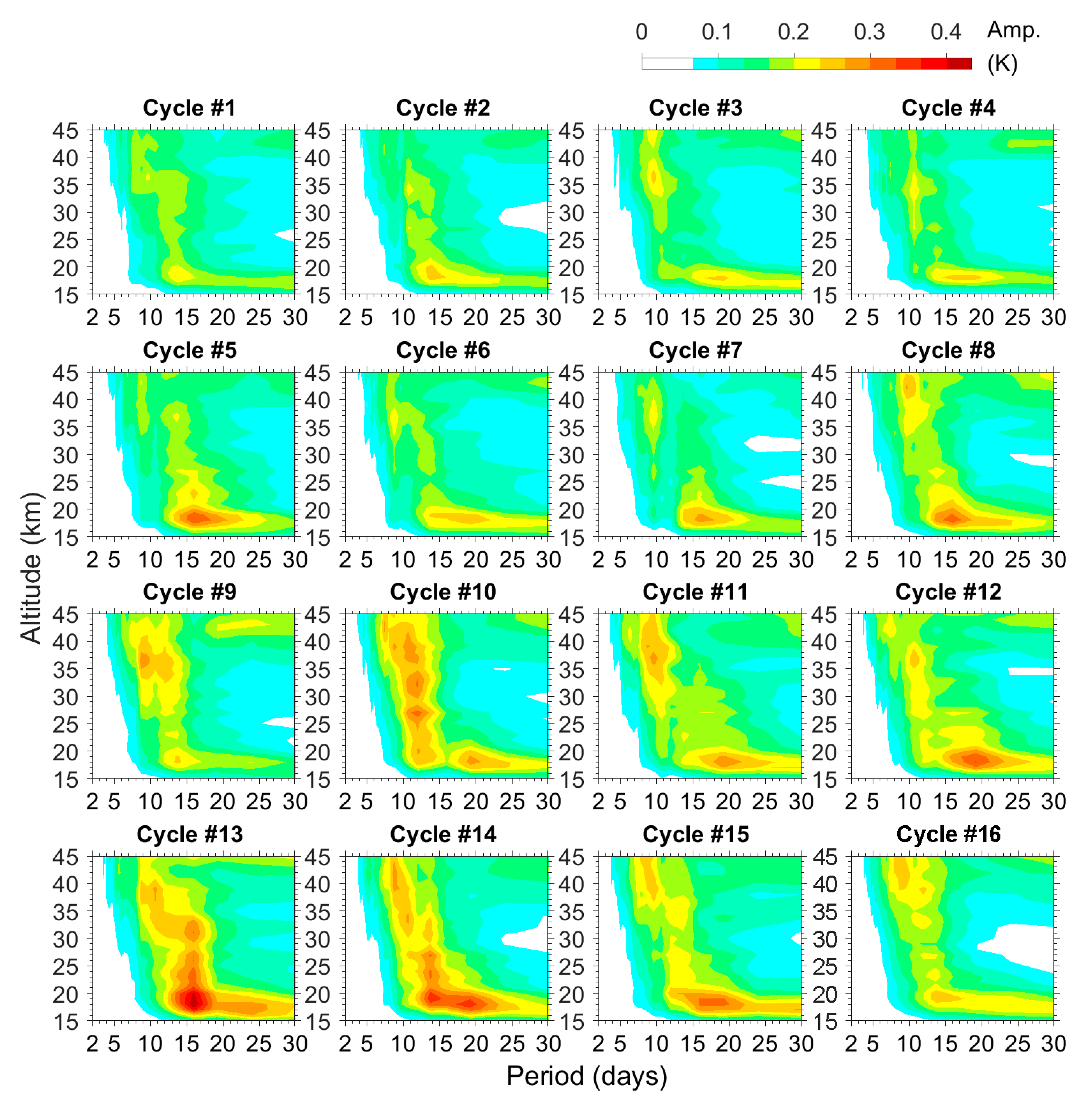
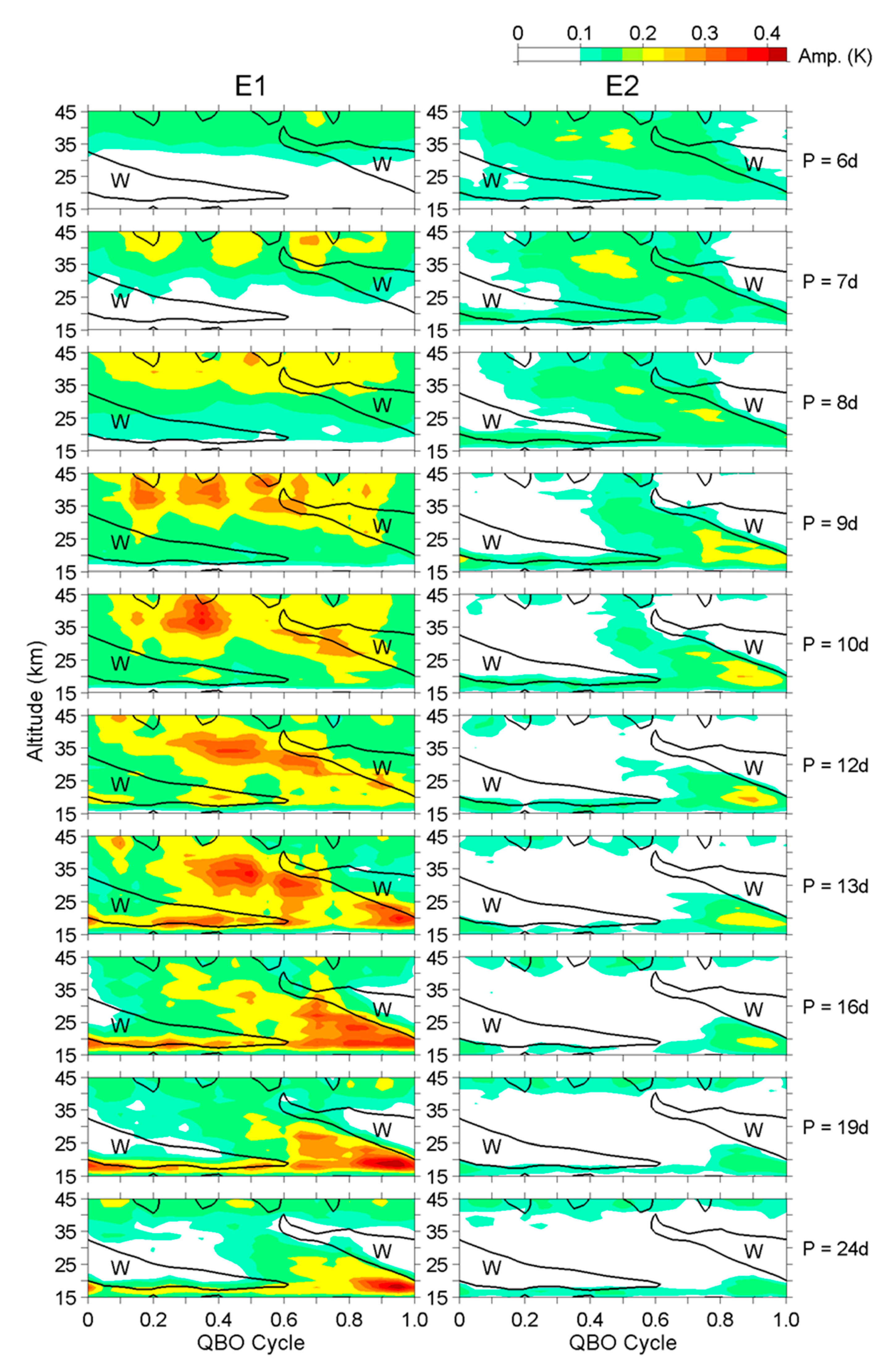
The temporal variations of E1 and E2 waves. Both inter-cycle and intra-cycle variations were found in the present study. The inter-cycle variations present in two ways. The wave amplitudes are more intense during several individual QBO cycles and also amplified after Cycle #8 that starts from May 1997. The intra-cycle variation is related to the zonal wind, so it also reveals the spatio-temporal evolution of wave amplitudes. The dominant wave period in the stratosphere varies throughout a QBO cycle. Faster waves that have a shorter wave period can penetrate the westerly regimes in the lower stratosphere, so they appear in the upper stratosphere during almost the whole QBO cycle. Those waves are mainly E1 waves with 6–10 day periods and E2 waves with 6 day periods that have a wavelength longer than the thickness of the westerly regime. In contrast, other slower waves that have a longer wave period and a shorter vertical wavelength cannot penetrate the westerly regime, and they are only active below the westerly shear in the lower and middle stratosphere during the last half of a QBO cycle.

(2)

Wave-mean flow interactions. The correlation analysis generally showed high correlations between the easterly wind and E1/E2 waves with various periods. Most E1 and E2 waves amplify to their maximum amplitudes after the maximum of easterly within a lag of 0.2 of a QBO cycle (~6 months). The lag decreases as the altitude decreases and further becomes zero at the bottom of the stratosphere (i.e., just above the tropopause). Exceptions are the E1 waves with 6–10 day periods—they have lower correlations with longer lags. Another correlation analysis between the E1/E2 waves and the acceleration of zonal wind also showed high correlations. The maximum westerly acceleration occurs ~0.1 QBO cycle (~3 months) after the maximum amplitudes of most E1 and E2 waves. Exceptions are again E1 waves with 6–10 day periods.

(3)

Correlations between the convective indices and the wave amplitudes. The 16-day E1 and E2 amplitudes during the epoch 2006–2013 were correlated to the Niño 3.4 index, the OLR, and the precipitation, but not the CAPE, over the examined Niño 3.4 region. The precipitation was further the most crucial one as it is able to represent the variation in wave amplitudes, though this part is a case study. In addition, inter-cycle variations, as summarized in (2), are considered to correlate with several El Niño events and the long-term increase in SST after Cycle #8 through the enhancement of convective activity.

The present study is the first long-term (40 years) investigation into the properties of Kelvin waves with wavenumbers 1 and 2 in the stratosphere; it also demonstrates a unique application of the ERA-Interim reanalysis dataset. The results and knowledge gained about Kelvin waves and their relationships with zonal wind as well as convections will help us in the future to diagnose anomalous events such as wave enhancements and the fast descending of westerly QBO.

References

1. Holton, J.R.; Hakim, G.J. An Introduction to Dynamic Meteorology, 5th ed.; Academic Press: Amsterdam, The Netherlands, 2012. [Google Scholar] [CrossRef]
2. Matsuno, T. Quasi-Geostrophic Motions in the Equatorial Area. J. Meteorol. Soc. Jpn. 1966, 44, 25–43. [Google Scholar] [CrossRef] [Green Version]
3. Holton, J.R.; Lindzen, R.S. A note on “Kelvin” waves in the atmosphere. Mon. Weather Rev. 1968, 96, 385–386. [Google Scholar] [CrossRef] [Green Version]
4. Wallace, J.M.; Kousky, V.E. Observational evidence of Kelvin waves in tropical stratosphere. J. Atmos. Sci. 1968, 25, 900–907. [Google Scholar] [CrossRef] [Green Version]
5. Alexander, S.P.; Tsuda, T.; Kawatani, Y.; Takahashi, M. Global distribution of atmospheric waves in the equatorial upper troposphere and lower stratosphere: COSMIC observations of wave mean flow interactions. J. Geophys. Res. 2008, 113, D24115. [Google Scholar] [CrossRef]
6. Chen, W.S.; Pan, C.J.; Das, U. The mean zonal wind effect on the long-term variation of ultra-fast Kelvin waves in the mesosphere and lower thermosphere and in the upper stratosphere. J. Atm. Sol.-Terr. Phys. 2018, 179, 459–467. [Google Scholar] [CrossRef]
7. Das, U.; Pan, C.J. Equatorial atmospheric Kelvin waves during El Niño episodes and their effect on stratospheric QBO. Sci. Total Environ. 2016, 544, 908–918. [Google Scholar] [CrossRef] [PubMed]
8. Hirota, I. Equatorial waves in upper stratosphere and mesosphere in relation to semiannual oscillation of zonal wind. J. Atmos. Sci. 1978, 35, 714–722. [Google Scholar] [CrossRef] [Green Version]
9. Kovalam, S.; Vincent, R.A.; Reid, I.M.; Tsuda, T.; Nakamura, T.; Ohnishi, K.; Nuryanto, A.; Wiryosumarto, H. Longitudinal variations in planetary wave activity in the equatorial mesosphere. Earth Plants Space 1999, 51, 665–674. [Google Scholar] [CrossRef] [Green Version]
10. Lott, F.; Denvil, S.; Butchart, N.; Cagnazzo, C.; Giorgetta, M.A.; Hardiman, S.C.; Manzini, E.; Krismer, T.; Duvel, J.-P.; Maury, P.; et al. Kelvin and Rossby-gravity wave packets in the lower stratosphere of some high-top CMIP5 models. J. Geophys. Res. 2014, 119, 2156–2173. [Google Scholar] [CrossRef] [Green Version]
11. Pan, C.J.; Uma, D.; Yang, S.S.; Wong, C.J.; Lai, H.C. Investigation of Kelvin Waves in the Stratosphere Using FORMOSAT-3/COSMIC Temperature Data. J. Meteorol. Soc. Jpn. 2011, 89, 83–96. [Google Scholar] [CrossRef] [Green Version]
12. Riggin, D.M.; Fritts, D.C.; Tsuda, T.; Nakamura, T.; Vincent, R.A. Radar observations of a 3-day Kelvin wave in the equatorial mesosphere. J. Geophys. Res. 1997, 102, 26141–26157. [Google Scholar] [CrossRef]
13. Salby, M.L.; Hartmann, D.L.; Bailey, P.L.; Gille, J.C. Evidence for equatorial kelvin modes in NIMBUS-7 LIMS. J. Atmos. Sci. 1984, 41, 220–235. [Google Scholar] [CrossRef] [Green Version]
14. Sridharan, S.; Tsuda, T.; Nakamura, T.; Kozu, T.; Mori, S.; Russell, J.M. Observations of the 7-day Kelvin wave in the tropical atmosphere during the CPEA campaign. J. Meteorol. Soc. Jpn. 2006, 84, 259–275. [Google Scholar] [CrossRef] [Green Version]
15. Suzuki, J.; Shiotani, M.; Nishi, N. Lifetime and longitudinal variability of equatorial Kelvin waves around the tropical tropopause region. J. Geophys. Res. 2010, 115, D03103. [Google Scholar] [CrossRef] [Green Version]
16. Das, U.; Pan, C.J. Strong Kelvin wave activity observed during the westerly phase of QBO—A case study. Ann. Geophys. 2013, 31, 581–590. [Google Scholar] [CrossRef] [Green Version]
17. Abdu, M.A.; Brum, C.G.M.; Batista, P.P.; Gurubaran, S.; Pancheva, D.; Bageston, J.V.; Batista, I.S.; Takahashi, H. Fast and ultrafast Kelvin wave modulations of the equatorial evening F region vertical drift and spread F development. Earth Planets Space 2015, 67, 1. [Google Scholar] [CrossRef] [Green Version]
18. Chang, L.C.; Palo, S.E.; Liu, H.-L.; Fang, T.-W.; Lin, C.S. Response of the thermosphere and ionosphere to an ultra fast Kelvin wave. J. Geophys. Res. 2010, 115, A00G04. [Google Scholar] [CrossRef] [Green Version]
19. Takahashi, H.; Wrasse, C.M.; Fechine, J.; Pancheva, D.; Abdu, M.A.; Batista, I.S.; Lima, L.M.; Batista, P.P.; Clemesha, B.R.; Schuch, N.J.; et al. Signatures of ultra fast Kelvin waves in the equatorial middle atmosphere and ionosphere. Geophys. Res. Lett. 2007, 34, L11108. [Google Scholar] [CrossRef] [Green Version]
20. Ern, M.; Preusse, P. Quantification of the contribution of equatorial Kelvin waves to the QBO wind reversal in the stratosphere. Geophys. Res. Lett. 2009, 36, L21801. [Google Scholar] [CrossRef] [Green Version]
21. Holton, J.R. On the frequency distribution of atmospheric Kelvin waves. J. Atmos. Sci. 1973, 30, 499–501. [Google Scholar] [CrossRef] [Green Version]
22. Salby, M.L.; Garcia, R.R. Transient response to localized episodic heating in the tropics. Part I: Excitation and short-time near-field behavior. J. Atmos. Sci. 1987, 44, 458–498. [Google Scholar] [CrossRef] [Green Version]
23. Wheeler, M.; Kiladis, G.N. Convectively coupled equatorial waves: Analysis of clouds and temperature in the wavenumber-frequency domain. J. Atmos. Sci. 1999, 56, 374–399. [Google Scholar] [CrossRef]
24. Kiladis, G.N.; Wheeler, M.C.; Haertel, P.T.; Straub, K.H.; Roundy, P.E. Convectively coupled equatorial waves. Rev. Geophys. 2009, 47, RG2003. [Google Scholar] [CrossRef]
25. Hayashi, Y. Space-time spectral analysis and its applications to atmospheric waves. J. Meteorol. Soc. Jpn. 1982, 60, 156–171. [Google Scholar] [CrossRef] [Green Version]
26. Dee, D.P.; Uppala, S.M.; Simmons, A.J.; Berrisford, P.; Poli, P.; Kobayashi, S.; Andrae, U.; Balmaseda, M.A.; Balsamo, G.; Bauer, P.; et al. The ERA Interim reanalysis: Configuration and performance of the data assimilation system. Q. J. R. Meteorol. Soc. 2011, 137, 553–597. [Google Scholar] [CrossRef]
27. L60 Model Level Definition. Available online: https://www.ecmwf.int/en/forecasts/documentation-and-support/60-model-levels (accessed on 15 September 2019).
28. Randel, W.J.; Wu, F. Kelvin wave variability near the equatorial tropopause observed in GPS radio occultation measurements. J. Geophys. Res. 2005, 110, D03102. [Google Scholar] [CrossRef]
29. Huang, B.; Thorne, P.W.; Banzon, V.F.; Boyer, T.; Chepurin, G.; Lawrimore, J.H.; Menne, M.J.; Smith, T.M.; Vose, R.S.; Zhang, H.-M. Extended Reconstructed Sea Surface Temperature, Version 5 (ERSSTv5): Upgrades, Validations, and Intercomparisons. J. Clim. 2017, 30, 8179–8205. [Google Scholar] [CrossRef]
30. Historical El Nino/La Nina Episodes (1950-present). Available online: https://origin.cpc.ncep.noaa.gov/products/analysis_monitoring/ensostuff/ONI_v5.php (accessed on 1 August 2019).
31. Graham, N.E.; Barnett, T.P. Sea Surface Temperature, Surface Wind Divergence, and Convection over Tropical Oceans. Science 1987, 238, 657–659. [Google Scholar] [CrossRef]
32. Knutson, T.R.; Weickmann, K.M. 30–60 Day Atmospheric Oscillations: Composite Life Cycles of Convection and Circulation Anomalies. Mon. Weather Rev. 1987, 115, 1407–1436. [Google Scholar] [CrossRef]
33. NOAA Interpolated Outgoing Longwave Radiation (OLR). Available online: https://www.esrl.noaa.gov/psd/data/gridded/data.interp_OLR.html (accessed on 28 July 2019).
34. Liebmann, B.; Smith, C.A. Description of a Complete (Interpolated) Outgoing Longwave Radiation Dataset. Bull. Am. Meteorol. Soc. 1996, 77, 1275–1277. [Google Scholar] [CrossRef] [Green Version]
35. Brunt, D. Physical & Dynamical Meteorology; The University Press: Cambridge, UK, 1939. [Google Scholar]
36. Adler, R.F.; Huffman, G.J.; Chang, A.; Ferraro, R.; Xie, P.-P.; Janowiak, J.; Rudolf, B.; Schneider, U.; Curtis, S.; Bolvin, D.; et al. The Version-2 Global Precipitation Climatology Project (GPCP) Monthly Precipitation Analysis (1979–Present). J. Hydrometeorol. 2003, 4, 1147–1167. [Google Scholar] [CrossRef]
37. GPCP Version 2.3 Combined Precipitation Data Set. Available online: https://www.esrl.noaa.gov/psd/data/gridded/data.gpcp.html (accessed on 29 July 2019).
38. Venkat Ratnam, M.; Tsuda, T.; Kozu, T.; Mori, S. Long-term behavior of the Kelvin waves revealed by CHAMP/GPS RO measurements and their effects on the tropopause structure. Ann. Geophys. 2006, 24, 1355–1366. [Google Scholar] [CrossRef] [Green Version]
39. Baldwin, M.P.; Gray, L.J.; Dunkerton, T.J.; Hamilton, K.; Haynes, P.H.; Randel, W.J.; Holton, J.R.; Alexander, M.J.; Hirota, I.; Horinouchi, T.; et al. The quasi-biennial oscillation. Rev. Geophys. 2001, 39, 179–229. [Google Scholar] [CrossRef]
40. de la Torre, A.; Alexander, P.; Giraldez, A. The kinetic to potential energy ratio and spectral separability from high-resolution balloon soundings near the Andes Mountains. Geophys. Res. Lett. 1999, 26, 1413–1416. [Google Scholar] [CrossRef]
41. VanZandt, T.E. A model for gravity wave spectra observed by Doppler sounding systems. Radio Sci. 1985, 20, 1323–1330. [Google Scholar] [CrossRef] [Green Version]
42. Ahrens, C.D.; Henson, R. Meteorology Today, 12th ed.; Brooks/Cole, Cengage Learning: Belmont, CA, USA, 2019. [Google Scholar]
Figure 1. The phase of the daily ERA-Interim zonal mean zonal wind over the equatorial (±10°) region during the study period of 1979–2019. The mark “W” stands for westerly and “E” stands for easterly. The dotted line indicates a 20 km altitude, and the dashed lines divide different quasi-biennial oscillation (QBO) cycles, where each cycle starts and ends when the corresponding westerly shear descends to a 20 km altitude. The identification number of each QBO cycle is also presented.
Atmosphere 11 00421 g001
Figure 2. The amplitudes of wavenumber 1 (E1) waves as a function of period and altitude (period–altitude spectra) during different QBO cycles, as defined and indicated in Figure 1.
Atmosphere 11 00421 g002
Figure 3. The amplitudes of E1 waves as a function of time and altitude. Each panel plots the amplitude at the wave period specified on the right-hand side of the panel. The zero-wind contours are also plotted by black lines.
Atmosphere 11 00421 g003
Figure 4. Same as in Figure 2, but showing the amplitudes of wavenumber 2 (E2) waves with a different color axis scaling.
Atmosphere 11 00421 g004
Figure 5. Same as in Figure 3, but showing the amplitudes of E2 waves with a different color axis scaling.
Atmosphere 11 00421 g005
Figure 6. The time-averaged amplitudes of E1 and E2 waves (columns) at periods ranging from 6 to 24 days (rows). The elapsed time is standardized to 0–1 QBO cycle (~29.4 months). The zero-wind of the time-averaged zonal wind is also plotted by black lines in each panel, and the westerly regimes of the time-averaged zonal wind are identified.
Atmosphere 11 00421 g006
Figure 7. The linear cross correlation coefficients between the time-averaged zonal wind and the wave amplitudes in a layout that is similar to Figure 6. Black, magenta, and white lines circle regions where the correlation coefficient is less than 0, −0.5, and −0.8, respectively. Gray lines indicate zero lag.
Atmosphere 11 00421 g007
Figure 8. The linear cross correlation coefficients between the time-averaged wave amplitudes and the acceleration of zonal wind in a layout that is similar to Figure 7. Black, green, and white lines circle regions where the correlation coefficient is greater than 0, 0.5, and 0.8, respectively. Gray lines indicate zero lag.
Atmosphere 11 00421 g008
Figure 9. (a) Vertical wavenumbers and (b) amplitudes of the E1 waves with 6–24 day periods at a 30 km altitude. (c) Amplitudes of E1 waves and (d) normalized zonal acceleration as functions of period and altitude.
Atmosphere 11 00421 g009
Figure 10. (top two panels) The amplitudes of the 16-day E1 and E2 waves as a function of time and altitude. The zero-wind contours are also plotted by black lines, and the westerly regimes are identified. (bottom four panels) The time series of the Niño 3.4 index, OLR, CAPE, and precipitation over the Niño 3.4 region (5°N–5°S, 120°–170°W). The dashed red line and blue line in the Niño 3.4 panel indicate the ±0.5°C criterions for El Niño and La Niña events, respectively.
Atmosphere 11 00421 g010
Figure 11. The linear cross correlation coefficients between (a,b) the Niño 3.4 index; (c,d) OLR; (e,f) CAPE; (g,h) precipitation and the 16-day E1/E2 amplitudes, respectively. Black and green lines circle regions where the correlation coefficient is greater than 0 and 0.5, respectively. Gray lines indicate zero lag.
Atmosphere 11 00421 g011