Article

Turbulence in a Coronal Loop Excited by Photospheric Motions

1
Dipartimento di Fisica, Università della Calabria, via P. Bucci, 87036 Rende, Italy
2
Radboud Radio Lab, Department of Astrophysics/IMAPP-Radboud University, P.O. Box 9010, 6500GL Nijmegen, The Netherlands
3
LESIA, Observatoire de Paris, Université PSL, CNRS, Sorbonne Université, Université de Paris, 5 place Jules Janssen, F-92195 Meudon, France
4
Department of Physics, University of Oslo, 1048 Blindern, 0316 Oslo, Norway
*
Author to whom correspondence should be addressed.
Atmosphere 2020, 11(4), 409; https://doi.org/10.3390/atmos11040409
Submission received: 15 March 2020 / Revised: 10 April 2020 / Accepted: 15 April 2020 / Published: 20 April 2020

Abstract

:
Photospheric motions are believed to be the source of coronal heating and of velocity fluctuations detected in the solar corona. A numerical model, based on the shell technique applied on reduced magnetohydrodynamics equations, is used to represent energy injection due to footpoint motions, storage and dissipation of energy in a coronal loop. Motions at the loop bases are simulated by random signals whose frequency-wavenumber spectrum reproduces features of photospheric motions: the p-mode peak and the low-frequency continuum. Results indicate that a turbulent state develops, dominated by magnetic energy, where dissipation takes place in an intermittent fashion. The nonlinear cascade is mainly controlled by velocity fluctuations, where resonant modes are dominant at high frequencies. Low frequency fluctuations present a power-law spectra and a bump at p-mode frequency; similar features are observed in velocity spectra detected in the corona. For typical loop parameters the energy input flux is comparable with that necessary to heat the quiet-Sun corona.

1. Introduction

The solar corona is the most external, rarefied and hottest part of the Sun’s atmosphere, which is formed by a plasma at an average temperature of the order of or larger than T 10 6 K. It is permeated by a strongly inhomogeneous magnetic field which is generated by the dynamo mechanism [1,2,3,4,5,6,7] operating in the solar convection zone. Among coronal magnetic structures, coronal loops represent a common configuration. The problem of elucidating the physical mechanisms which are responsible for the energization of the solar corona and its consequent heating has been widely studied from a theoretical point of view. One of the possible sources of energy for the corona is represented by mechanical motions in the photosphere, which is the lowest and most dense part of the solar atmosphere. The energy associated with these motions, after crossing the chromosphere [8], would be partially transferred to the rarefied corona through the magnetic field which is rooted in the photosphere and ubiquitously fills the corona. Two important issues still under debate are the following: (i) in which form and at which timescales does the energy of photospheric motions reaches the corona? (ii) How is this energy moved to the very small scales where it can be dissipated? This paper aims to give a contribution to both points.
Concerning the first question, models of coronal heating have been traditionally classified into two groups: “direct current” (DC) or “alternating current” (AC). In the former case, slow photospheric motions are considered, with timescales longer than the Alfvén crossing time t A , which is the time a perturbation takes to cross a closed magnetic structure propagating at the Alfvén velocity. In that case, coronal structures continuously re-arrange through a sequence of quasi-equilibrium states. Magnetic energy increases in time until reaching a threshold when it is suddenly dissipated, while the kinetic energy remains at a much lower level. In contrast, AC heating models consider perturbations at timescales comparable to or shorter than t A , essentially belonging to the Alfvén branch, where kinetic energy is of the order of magnetic energy. Indeed, quasi-periodic plasma velocity fluctuations have been ubiquitously detected in corona, propagating along the magnetic field with velocities compatible with the Alfvén speed [9,10,11]. The frequency f of such fluctuations spans a wide range, going from f 10 4 Hz t A 1 to f 2 × 10 2 Hz t A 1 . The frequency range of detected photospheric motions is as much as wide [12,13]. Observations also suggest the existence of velocity fluctuations in the corona at much higher frequencies, based on measurements of non-thermal broadenings of coronal lines [14]. Therefore, the distinction between AC or DC mechanisms appears to be quite artificial, since both kind of processes are probably at work at the same time [15]. In the present paper we will consider a situation where the frequency range of excited fluctuations covers both kind of phenomena.
Energy injected in the corona needs to be transferred to small dissipative scales in order to be converted into heat. Concerning this second question, different possibilities have been studied about the involved mechanism. Some of them are related to spatial inhomogeneities of the coronal structures that generate small scales in the perturbations propagating inside them, both within a fluid approach [16,17,18,19,20,21,22,23,24,25,26] and taking into account kinetic effects [27,28]. These models consider the coupling between perturbations and a nonuniform background. In contrast, nonlinear couplings among perturbations are at the base of turbulence models, which describe the formation of an energy cascade that transfers fluctuation energy to small dissipative scales [29,30,31,32,33,34,35,36,37,38,39]. Evaluations of energy balance between injected flux and spectral transfer has also been carried out in direct simulations [40,41,42]. More recently, models taking into account both turbulence and inhomogeneities have been proposed [43]. Related to the heating problem, other aspects have also been considered in the dynamics of a coronal loop, such as the complexity of magnetic topology induced by motions at its ends [44], or kink and Alfvénic torsional mode interactions [45,46,47].
Some of the above-cited papers are concerned with direct numerical simulation of magnetohydrodynamic (MHD) equations, and based on first principles. However, due to numerical limitations, the wide range of spatial scales of coronal turbulence is not adequately described. This problem can be circumvented using “reduced” models of turbulence, like the so-called shell models [30,31,48], in which the dynamics of turbulence is represented in a simplified Fourier space. In a coronal context, hybrid shell models have been developed [33,37], based on Reduced MHD (RMHD) [49,50]. In such models the spatial dependence on the coordinate along the background magnetic field is retained, which allows one to impose boundary conditions at the coronal base. This approach is more appropriate with respect to classical shell models, since it is believed that the energization of the coronal structures is due to motions at the coronal base. Hybrid shell models have successfully reproduced statistical properties of coronal energy release events [33], as well as the energy flux [38,39] necessary to maintain the corona at the observed temperature [51]. Moreover, they predict fluctuating velocity enhancements associated with loop resonance [38,39], which can be related to increases of the spectral energy flux [39] and to triggering of solar flares [34,35].
In references [33,35] a time dependent velocity has been imposed at the loop bases at the largest transverse scales, with a correlation time of the order of t c o r r = 300 s, corresponding to the typical time of photospheric p-modes. In the present study we perform numerical simulations of turbulence in a coronal loop, by means of the same hybrid shell model as in [33,35], but using different boundary conditions. In particular, the presently adopted boundary conditions try to give a more realistic representation of the spatial and temporal dependence of photospheric motions. They are based on detailed space-time measurement of the photospheric velocity field [12,13]. Beside p-modes, the corresponding frequency spectra display also oscillations at much lower frequencies, with different contributions at different spatial scales. The aim of the present study is to elucidate to which extent a more realistic representation of photospheric motions driving coronal loop oscillations can affect the results, in terms of loop frequency spectra, resonance triggering, level of oscillations and incoming energy flux. These results are relevant in the perspective of obtaining a more realistic modeling of the turbulence dynamics in a coronal loop.

2. Modelling Turbulence and Boundary Motions in a Coronal Loop

In this section we briefly describe the model we adopted to represent the turbulence in a coronal loop, and how boundary conditions at the loop bases have been implemented. More details on the numerical model can be found in reference [33].

2.1. The Hybrid Shell Model

We consider a simplified representation of a coronal loop, where the loop curvature is neglected. We use a Cartesian reference frame in which the x axis is parallel to the loop axis, and we represent the loop as an elongated parallelepiped, with longitudinal length L | | and perpendicular width L , equal in both transverse y and z directions, such that L | | L . The numerical model is based on RMHD equations. In this context it is assumed that the loop is permeated by a strong uniform longitudinal magnetic field B 0 = B 0 e x , with B 0 constant and e x indicating the unit vector in the parallel direction. Small-amplitude magnetic field perturbations δ B are superposed on the background magnetic field B 0 : δ B B 0 . Moreover, the longitudinal spatial scale | | of perturbations is assumed to be much larger than the perpendicular scale: | | . Under these assumptions the RMHD equations can be derived [49,50]. They can be written in the following dimensionless form:
Z ± t Z ± x + Z · Z ± + p = χ 2 Z ± ,
· Z ± = 0 ,
where Z ± = v ± b are the Elsässer variables; v and b are the transverse components of velocity and magnetic field normalized to c A and B 0 , respectively; c A = B 0 / ( 4 π ρ 0 ) 1 / 2 is the Alfvén velocity and ρ 0 is the background uniform mass density; p is the total (kinetic + magnetic) pressure, normalized to B 0 2 / 4 π . Lengths are normalized to the loop longitudinal size L | | , time t is normalized to the Alfvén crossing time t A . The dissipation coefficient is χ = μ / ( c A L | | ) where the magnetic diffusivity μ has been assumed equal to the kinematic viscosity ν . Equation (2) implies that transverse motions are non-compressive, while Equation (1) indicates that propagation take place in the longitudinal direction at the Alfvén speed.
The above equations are the basis to derive the hybrid shell model [33]. First, Equations (1) and (2) are Fourier-transformed with respect to the transverse coordinates, while the dependence on the longitudinal coordinate x is kept. The underlying assumption is that the turbulent fluctuations are statistically homogeneous in the transverse directions. In particular, the transverse structuring of the loop is neglected in the present simplified model. Then, the k plane is divided into concentric shells of exponentially growing radius. For each shell a single scalar value k n = k 0 2 n of the wavevector and a scalar complex value Z n ± ( x , t ) of the transformed Elsässer variables are defined, where k 0 = 2 π ( L | | / L ) = 2 π / R is the fundamental dimensionless wavevector, R = L | | / L is the loop aspect ratio, n = 0 , . . . , n m a x , with n m a x + 1 the number of shells. Convolution products corresponding to nonlinear terms in Equation (1) are represented by products between variables Z n ± ( x , t ) belonging to nearest or next nearest neighbor shells. Finally, the coefficients of such products are determined by imposing that nonlinear terms conserve the 2D quadratic invariants: total energy, cross-helicity and squared magnetic potential [30]. The final form of the hybrid shell model equations is the following [33]:
t x Z n ± = i k n 13 24 Z n + 2 ± Z n + 1 + 11 24 Z n + 2 Z n + 1 ± 19 48 Z n + 1 ± Z n 1 11 48 Z n + 1 Z n 1 ± + 19 96 Z n 1 ± Z n 2 13 96 Z n 1 Z n 2 ± * χ k n 2 Z n ± ,
where i is the imaginary unit and the asterisk indicates complex conjugate. The expression (3) represents a system of coupled partial differential equations. We used an initial condition corresponding to an unpertubed loop: Z n ± ( x , t = 0 ) = 0 . Boundary conditions must be given at the two loop ends: x = 0 and x = 1 . Since Equation (3) describe the propagation of Z n ( Z n + ) along the positive (negative) x direction, at each boundary only the value of the “incoming” variable can be imposed. On the other hand, at boundaries we want to impose the value of the (transverse) velocity, which represents how photospheric motions solicitate the two loop ends. This is done by expressing the velocity in terms of the Elsässer variables; therefore, the expression of incoming variables at the two boundaries are:
Z n ( x = 0 , t ) = 2 u L , n ( t ) Z n + ( x = 0 , t ) ,
Z n + ( x = 1 , t ) = 2 u R , n ( t ) Z n ( x = 1 , t ) ,
where the complex functions u L , n ( t ) and u R , n ( t ) represent the velocity perturbation of the n-th shell at the boundaries x = 0 (left) and x = 1 (right), respectively, and will be specified later. The Elsässer variables Z n ± corresponding to perturbations leaving the spatial domain are determined by the evolution Equation (3) inside the domain. We notice that the value of magnetic field fluctuation at the two boundaries can be expressed as a combination of the velocity and of the “outcoming” Elsässer variable: b n ( x = 0 , t ) = Z n + ( x = 0 , t ) + u L , n ( t ) and b n ( x = 1 , t ) = u R , n ( t ) Z n ( x = 1 , t ) . While we impose u L , n ( t ) and u R , n ( t ) , we cannot impose anything about the outcoming Elsässer variables. Therefore, in our case the magnetic field fluctuation at boundaries is partially determined by the velocity and partially by the internal dynamics.
The system (3) of 2 ( n m a x + 1 ) coupled partial differential equations, with complex unknowns Z n ± depending on x and t, has been numerically solved using a second-order centered finite-difference scheme in space and a second-order Runge-Kutta method in time. Since perturbations propagate along x with velocity ± c A (with c A = 1 in normalized units), the size Δ x of spatial grid has been chosen such that Δ x c A t n l ( k m a x ) , where k m a x = k 0 2 n m a x and the nonlinear time t n l ( k ) can be estimated assuming that fluctuations follow a Kolmogorov spectrum: t n l ± ( k m a x ) = 1 / ( Z 0 ± k 0 1 / 3 k m a x 2 / 3 ) . Being Z 0 ± b 0 < B 0 (see below), we finally set the value of Δ x satisfying the condition Δ x c A / ( B 0 k 0 1 / 3 k m a x 2 / 3 ) . The time step Δ t has been chosen such as to fulfil the CFL stability condition.
An energy balance equation can be derived from (3):
d E d t = P ( t ) W ( t ) ,
where E ( t ) , P ( t ) and W ( t ) are the total energy, the net power incoming through the boundaries and the total dissipated power, respectively:
E ( t ) = n 0 1 | Z n + ( x , t ) | 2 + | Z n ( x , t ) | 2 4 d x , W ( t ) = χ 2 n 0 1 k n 2 | Z n + ( x , t ) | 2 + | Z n ( x , t ) | 2 d x ,
P ( t ) = 1 4 n | Z n ( 0 , t ) | 2 | Z n + ( 0 , t ) | 2 + | Z n + ( 1 , t ) | 2 | Z n ( 1 , t ) | 2 .
We consider a configuration where the loop width is L = 10 4 km; the aspect ratio is R = 30 / ( 2 π ) , corresponding to a loop length L | | = 4 . 77 × 10 4 km; the Alfvén velocity is c A = 3 . 18 × 10 3 km/s (corresponding to a crossing time t A = 15 s), the background density is ρ 0 = 1 . 67 × 10 16 g cm 3 . Correspondingly, the value of the background magnetic field is B 0 = c A / ( 4 π ρ 0 ) 1 / 2 = 14 . 5 G. The loop sizes are slightly larger than those in Ref. [33] to adapt L to the wavelengths in photospheric data (see below), while both R and t A are the same as in [33]. The normalizing factors for energy and power are: E N = ρ 0 c A 2 L | | 3 / R 2 = 8 . 05 × 10 28 erg and W N = ρ 0 c A 3 L | | 2 / R 2 = 5 . 37 × 10 27 erg/s, respectively. The shell technique allows to describe a very extended spectrum with a relatively small computational effort. We set n m a x = 11 , corresponding to a spectral width k m a x / k 0 = 2 11 = 2048 , and χ = 10 7 .

2.2. Data Analysis

In the motions of the solar photosphere the convective dynamics coexists with the contribution of global solar oscillations. Among the latter, p-modes are acoustic oscillations in the frequency range ( 1 5 ) × 10 3 Hz, whose contribution in k ω Fourier spectra appears as a sequence of discrete ridges (e.g., ref. [12]). At lower frequencies another contribution is found, in form of a continuum, commonly attributed to the solar turbulent convection. However, there are indications, based on numerical simulations, that the low-frequency continuum can arise from the interaction between convection and g-mode global oscillations [52].
In order to set more realistic boundary conditions for the hybrid shell model, we consider a data analysis of the photospheric velocity field [12,13] performed over a dataset obtained from images acquired by the Michelson Doppler Imager (MDI) instrument mounted on the Solar and Heliospheric Observatory (SOHO) spacecraft. Images have a spatial resolution of 0 . 6 arcsec, corresponding to 435 km on the Sun’s surface, a time resolution of 60 s and the time series spans a period of duration 5 . 32 × 10 4 s. The corresponding frequency range is 1 . 9 × 10 5 Hz f 1 . 6 × 10 2 Hz. In the typical turbulence setup, energy is injected into the system at large spatial scales, denoted as “injection scales”. In our case, the mechanism supposed to inject energy into the corona are photospheric motions. We consider three distinct bands of wavelength λ in photospheric motions, which represent the injection scales of our model: band B0, corresponding to 7000 km λ 14 , 000 km; band B1, corresponding to 3500 km λ 7000 km; band B2, corresponding to 1750 km λ 3500 km. Motions in these bands are used to setup the boundary conditions at the loop bases in the first three shells: u 0 L , R , u 1 L , R , u 2 L , R are determined by motions in B0, B1, B2, respectively. We notice that the transverse wavelenght (in physical units) corresponding to the shell n = 0 is λ 0 = ( 2 π / k 0 ) L | | = L = 10 , 000 km; therefore, λ 0 is approximately located in the center of the length interval corresponding to band B0. Similarly, the wavelengths corresponding to the shells n = 1 and n = 2 are λ 1 = λ 0 / 2 = 5000 km and λ 2 = λ 0 / 4 = 2500 km, that are approximately located in the center of length intervals corresponding to bands B1 and B2, respectively.
In Figure 1 the frequency spectra U n ( f ) , n = 0 , 1 , 2 derived from the dataset, corresponding to the three spatial bands, are plotted. Each spectra is divided by the integrated energy U T = n U n ( f ) d f , and the frequency f is normalized to t A 1 . In each band a peak is present, centered at a f 0 . 05 and corresponding to the p-mode contribution, as well as the low-frequency continuum. The frequency-integrated energy decreases going from larger (B0) to smaller (B2) spatial scales; moreover, the p-modes to continuum contribution ratio also decreases from B0 to B2.

2.3. Boundary Conditions

To setup boundary conditions, we consider the following differential equation:
d u d t = Ω u + μ ( t ) ,
where u ( t ) is a complex function of time; Ω = 1 / T ± i ω 1 is a complex frequency, with T and ω 1 real constants; and μ ( t ) = μ R ( t ) + i μ I ( t ) is a complex function. Performing the Fourier transform of Equation (9) we find u ^ ( ω ) = μ ^ ( ω ) / 1 / T i ω ± ω 1 , where the “hat” indicate the Fourier transform. Therefore, the power spectrum of the solution of Equation (9) is given by:
| u ^ ( ω ) | 2 = | μ ^ ( ω ) | 2 ω ω 1 2 + 1 / T 2 = L ( ω ) | μ ^ ( ω ) | 2 ,
where L ( ω ) is a Lorentzian function of width 1 / T , centered at the frequency ± ω 1 . In our case, we choose μ R ( t ) and μ I ( t ) as random signals with null autocorrelation time, which have a flat power spectrum corresponding to a white noise. Approximating such a spectrum with a constant, it follows that the power spectrum | u ^ ( ω ) | 2 of the solution has a Lorentzian shape, given by L ( ω ) . Equation (9) is numerically solved by a finite-difference second-order scheme, and at each time step t i the values μ R ( t i ) and μ I ( t i ) are random numbers extracted from a uniform distribution. This procedure allows us to obtain a complex signal u ( t ) with an approximately Lorentzian spectrum, whose parameters (center frequency and width) can be tuned by choosing the values ω 1 and T.
For each of the three spatial bands B0, B1, B2, and for each boundary (left and right) we solve three equations of the form (9): for two of them we use opposite values of the central frequency ( ± ω 1 ); this is intended to reproduce the contribution of p-modes in the spectrum, in the form of a Lorentzian-shaped peak. For the third equation we set ω 1 = 0 , corresponding to a Lorentzian spectrum centered at the null frequency; it models the low-frequency component of the photospheric spectrum. The three functions obtained in this way are superposed at each time step with different amplitudes, finally getting the signals: u L , n ( t ) and u R , n ( t ) for the left and right boundary, respectively, which give the velocity imposed at the two loop ends for the first three shells. These are used in Equations (4) and (5). Since the single solutions are statistically independent, the power spectrum of these signals is given by the superposition of the three Lorentzian spectra. Therefore, the power spectrum of u L , n ( t ) and u R , n ( t ) has the following form:
F n ( ω ) = N 2 a n , 0 2 ω 2 + 1 / T n , 0 2 + a n , 1 2 1 ω ω n , 1 2 + 1 / T n , 1 2 + 1 ω + ω n , 1 2 + 1 / T n , 1 2 ,
where, for each band n, T n , 0 1 and T n , 1 1 are the widths of the Lorentzian functions; a n , 0 and a n , 1 are the corresponding amplitudes; ω n , 1 is the frequency of the peak and N is a normalization factor. The difference between the signals on the left and right boundary is only in the choice of the random number seeds which determine the random functions μ ( t ) . Since we used different random seeds for the three shells and for the two boundaries, all the functions u L , n ( t ) and u R , n ( t ) , n = 0 , 1 , 2 , are completely uncorrelated.
The values of the above parameters are reported in Table 1. They are chosen in a way to approximately reproduce the shape of the three spectra plotted in Figure 1. Correspondingly, the RMS value of the velocity at each end of the loop is u R M S = n | u L , n ( t ) | 2 t 1 / 2 = n | u R , n ( t ) | 2 t 1 / 2 = 1 . 25 × 10 3 in dimensionless units (angular parentheses indicate time average), corresponding to u R M S c A = 2 . 5 km/s, which is of the order of typically observed photospheric velocities. In Figure 1 the multiple Lorentzian spectra F n (dashed lines) are plotted along with the spectra of photospheric motions (full lines), for the three spatial bands B0, B1 and B2. We can see that multiple Lorentzian spectra approximately fit the corresponding photospheric velocity spectra. In Figure 2 the spectrum e v ( f ) = n = 0 n = 2 | u ^ R , n ( f ) | 2 of the velocity imposed at the boundary x = 0 is shown as a function of the frequency f. The velocity spectrum at the other boundary x = L is very similar and is not shown. The presence of the peak at f = 0 . 05 is clearly visible, as well as the low-frequency component. Such a spectrum is more noisy than the Lorentzian model (11) because the function μ ( t ) is obtained using a random-number generating routine which gives a signal with a spectrum that is flat on average, but with a certain amount of noise superposed.
The above-described method to generate boundary conditions is a generalization of that used in Ref. [33]. In that paper only the boundary at x = 0 was excited with a given velocity field at the first three shells: u L , n ( t ) 0 , n = 0 , 1 , 2 , while a vanishing velocity was imposed on the other boundary: u R , n ( t ) = 0 . Moreover the frequency spectra of u L , n ( t ) were all Lorentzian fuctions with center at ω = 0 and width corresponding to the p-mode frequency ( ( 300 s ) 1 ). Those spectra can be obtained from the expression (11) by setting a n , 1 = 0 and T n , 0 = π / 10 . It is clear that in the present case the spectra are much more similar to the photospheric velocity spectra than those used in Ref. [33].

3. Results

Due to the velocity imposed at the boundaries, energy is continuously injected into the domain in form of velocity and magnetic field fluctuations. The dynamics of such fluctuations is also determined by their propagation along the loop and by nonlinear interactions which move energy towards small scales, where it can be dissipated. In the top panel of Figure 3 the time dependence of the total energy E is plotted. It can be seen that the model does not predict a stationary level for the total energy E of the fluctuating fields inside the loop. On the contrary, E erratically varies during the time, reaching higher values E ( 2 4 ) × 10 28 erg in the time interval 60 h t 95 h, and a much lower level, roughly E 5 × 10 27 erg, during the interval 220 h t 320 h. This is due to the fact that the system is characterized by different dynamical regimes, that we will describe later in this section.
In consequence of intermittency—a peculiar feature of this system [53]—the dissipated power W displays abrupt bursts during the time (Figure 3) which are a signature of the fragmentation of dissipative structures taking place at small scales. The average value of the dissipated power is W t = 5 . 44 × 10 23 erg/s. Bursts of W can be identified as energy release events taking place in the solar corona. Indeed, it has been shown that some statistical properties of dissipative events in the hybrid shell model, namely, the distributions of peak intensity, duration time, released energy and waiting times between subsequent events, positively compare with the same distributions found for coronal energy release events [33].
The incoming power P varies on a very short time scale, assuming both positive and negative signs. In fact, the value of P depends on both inward and outward propagating modes (Equation (8)), i.e., P is determined not only by the boundary conditions but also by the internal dynamics. However, the average value P t = 5 . 60 × 10 23 erg/s is positive, indicating that, on average, motions imposed at the loop boundary have introduced energy inside the loop. We notice that P t W t , indicating that the incoming power is almost balanced by the dissipated power. A perfect balance is not reached because the energy E contained inside the loop is not stationary in time.
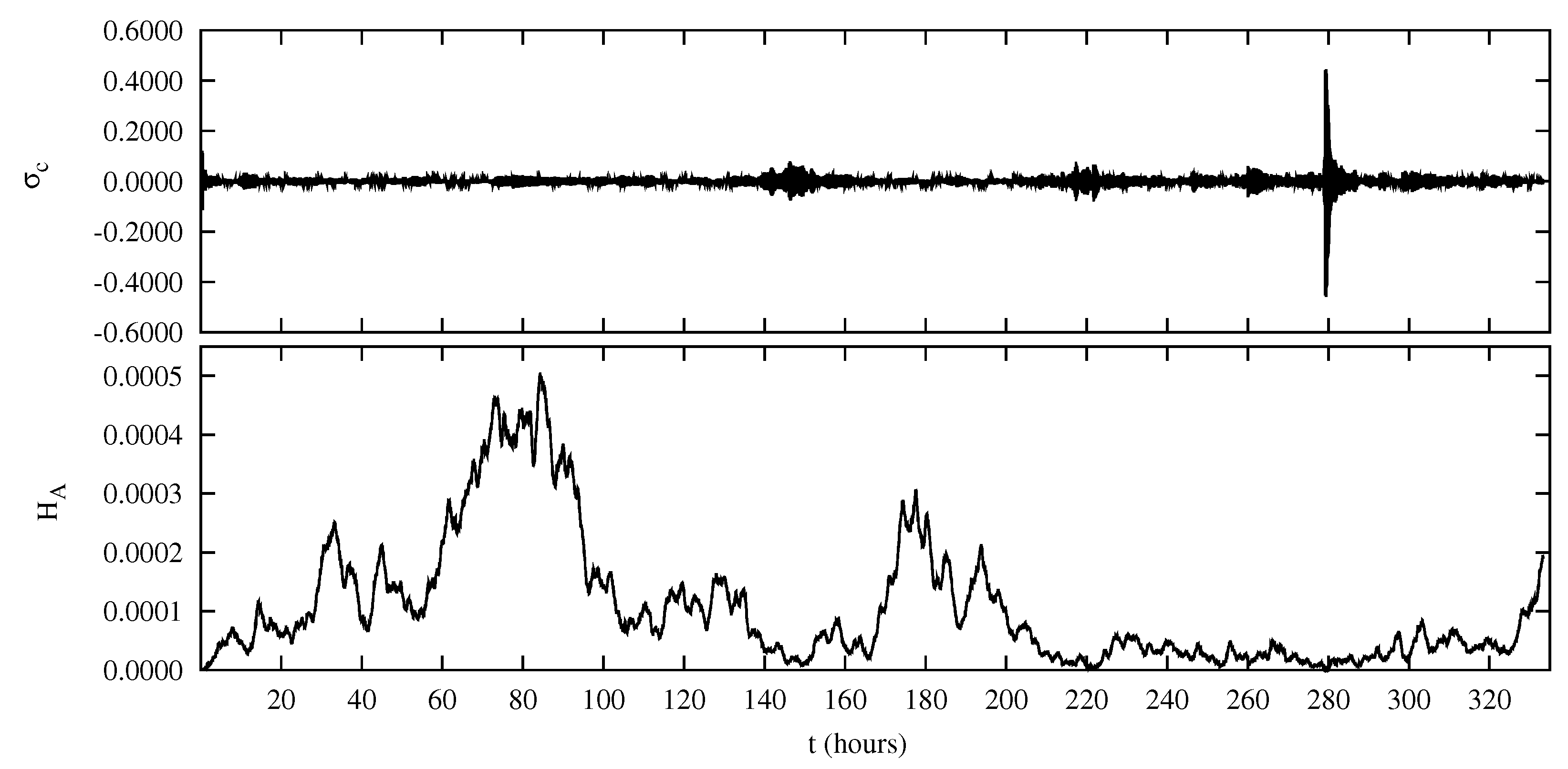
We calculated the normalized cross-helicity σ c = ( E + E ) / ( E + + E ) , where the pseudo-energies are defined by E ± = ( 1 / 4 ) n 0 1 | Z n ± | 2 d x . The normalized cross-helicity satisfies the condition | σ c | 1 ; in particular, it is σ c 1 ( σ c 1 ) when Z + ( Z ) fluctuations dominate on Z ( Z + ) fluctuations. In Figure 4 (upper panel) the normalized cross-helicity is plotted as a function of time. It can be seen that σ c is quite close to zero during almost all the simulation time, indicating that the level of Z + fluctuations is comparable with that of Z fluctuations. Indeed, we will show that the most energetic fluctuations are low-frequency magnetic fluctuations, where | v n | | b n | (in dimensionless units), this latter condition corresponding to | Z n + | | Z n + | . Therefore, the dominance of magnetic fluctuations is compatible with low | σ c | values. During a short interval around t 280 h, σ c displays fast oscillations where it changes sign on a short time scale, reaching values sensibly different form zero. During this phase of the time evolution the dominance of magnetic perturbations is temporarily suppressed, as testified by the particularly low value of the total energy E (Figure 3).
The squared magnetic potential, defined as H = ( 1 / 2 ) n 0 1 | b n / k n | 2 d x , is plotted as a function of time in the lower panel of Figure 4. Comparing with the total energy plotted in Figure 3 we see that H and E have a very similar time behaviour. This is again due to the dominance of large-scale magnetic fluctuations in determining E and to the fact that the major contribution to H comes from magnetic fluctuations at low k n values. We notice that both cross-helicity H c = E + E and squared magnetic potential H are ideal invariants of 2D shell models, i.e., they are exactly conserved by nonlinear terms in Equation (3). However, in the hybrid shell model H and H c are not conserved, both because of the driving imposed at boundaries x = 0 and x = 1 , and in consequence of dissipation.
In order to see how velocity and magnetic field fluctuations are on average distributed along the longitudinal extension x of the loop, we calculated the RMS of the velocity and magnetic field fluctuations as function of x, as in the following:
v R M S ( x ) = n = 0 n m a x | v n ( x , t ) | 2 t 1 / 2 , b R M S ( x ) = n = 0 n m a x | b n ( x , t ) | 2 t 1 / 2
where v n = ( Z n + + Z n ) / 2 and b n = ( Z n + Z n ) / 2 . These quantities are plotted in Figure 5, where time average has been performed over different intervals of time. In particular, we consider the RMS of both velocity and magnetic field fluctuations computed by considering the whole simulation time (black solid lines in Figure 5), for the interval 0 t 54 h (grey dot-dashed lines) and for the interval 58 h t 116 h (magenta dashed lines), respectively.
From Figure 5 we see that the velocity and magnetic field fluctuation levels averaged over the whole simulation are v R M S 5 × 10 6 cm s 1 and b R M S 5 G, respectively. We notice that b R M S / B 0 0 . 33 , which is sufficiently consistent with the assumptions of RMHD. The RMS values corresponds to fluctuating kinetic and magnetic energy densities: ε k = ρ 0 v R M S 2 / 2 2 × 10 3 erg cm 3 and ε m = b R M S 2 / ( 8 π ) 1 erg cm 3 . Therefore, the fluctuating magnetic energy is much larger than the kinetic one. This property is peculiar to models describing the DC coronal heating. Comparing the profiles in the two time intervals [ 0 h, 54 h] and [ 58 h, 116 h], we see that velocity fluctuations are larger when the total energy E is lower. Indeed, it has been shown [34,38] that a higher level of velocity fluctuations corresponds to a more efficient energy transfer from larger to smaller transverse scales. Therefore, the higher energy level in the interval [ 58 h, 116 h] can be interpreted as due to a lower velocity fluctuation level that partially inhibits the nonlinear cascade, allowing the energy—mostly magnetic energy—to accumulate at large scales. It is interesting to note that the velocity fluctuations in time interval [ 58 h, 116 h] are slightly lower than the average value computed on the whole simulation but certainly lower than those calculated in time interval [ 0 h, 54 h]. This highlights the high sensitivity of this system with respect to the velocity field fluctuations as regards the development of the nonlinear cascade and, consequently, of the intermittency. Moreover, since most of the energy E is of magnetic origin, it is not surprising that larger E corresponds to higher b R M S values. Finally, we observe that the spatial profile b R M S ( x ) is essentially flat, with small-amplitude modulations along x, while the v R M S ( x ) profile starts from values of the order of a few km/s at the two boundaries x = 0 km and x = 3 × 10 4 km, rapidly reaching v R M S 50–60 km/s inside the loop. The latter values are compatible with velocity measurements deduced by the nonthermal broadening of coronal spectral lines [14].
Analyzing the system in terms of input—embodied by the forcing velocity—and of output, i.e., the response of the system embodied by dynamically developed energy features, we examine the spectral kinetic and magnetic energies with their properties. These quantities are defined by
e v ( ω ) = n = 0 n m a x 0 L d x L | v ^ n ( x , ω ) | 2 , e b ( ω ) = n = 0 n m a x 0 L d x L | b ^ n ( x , ω ) | 2 ,
where v n ( x , t ) = ω v ^ n ( x , ω ) exp ( i ω t ) and b n ( x , t ) = ω b ^ n ( x , ω ) exp ( i ω t ) . They have been computed in two dynamically different time intervals, namely 0 h t 54 h and 58 h t 116 h.
The kinetic energy imposed at the boundaries through the forcing velocity displays the same features as observed in the data of the photospheric velocity (input of the system). In particular, a bump centered at frequency f = 0 . 05 , corresponding to (300 s) 1 , is reproduced in the frequency spectrum (see Figure 2). Correspondingly, the system responds by forming energy spectra with peculiar characteristics (see Figure 6 and Figure 7): a well-defined spike is present both in kinetic and magnetic spectra, centered at the fundamental resonant frequency f = 0 . 5 , i.e., inverse of the Alfvén crossing time t A , as well as subsequent spikes corresponding to the higher harmonics, at frequencies multiples of the fundamental one ( f = 1 , 1 . 5 , 2 , 2 . 5 , 3 , 3 . 5 , 4 ). Resonant modes are standing Alfvénic fluctuations which are excited by the broad-band spectrum of the boundary velocity [38,39]. All these spikes are very sharp and slender. The resonance phenomenon is related to partial reflection of fluctuations taking place at both boundaries x = 0 and x = 1 . Of course, since the net incoming flux P takes both positive and negative signs in time (Figure 3), the reflection is not total, otherwise no energy could enter or leave the spatial domain.
Another feature which is present both in kinetic and magnetic spectra is a broader peak centered at frequency f = 0 . 05 , corresponding to the analogous peak in the forcing velocity spectrum (Figure 2), which represents the contribution of p-modes. Therefore, the model predicts that a clear signature of this particular photospheric frequency should be found in the spectrum of plasma velocity up in the corona. We also verified that such frequency is present in the body of the loop, far from the boundaries: indeed, even including only the central part of the loop in the integration domain (see Equation (13), the peak at f = 0 . 05 in the resulting spectra is still present.
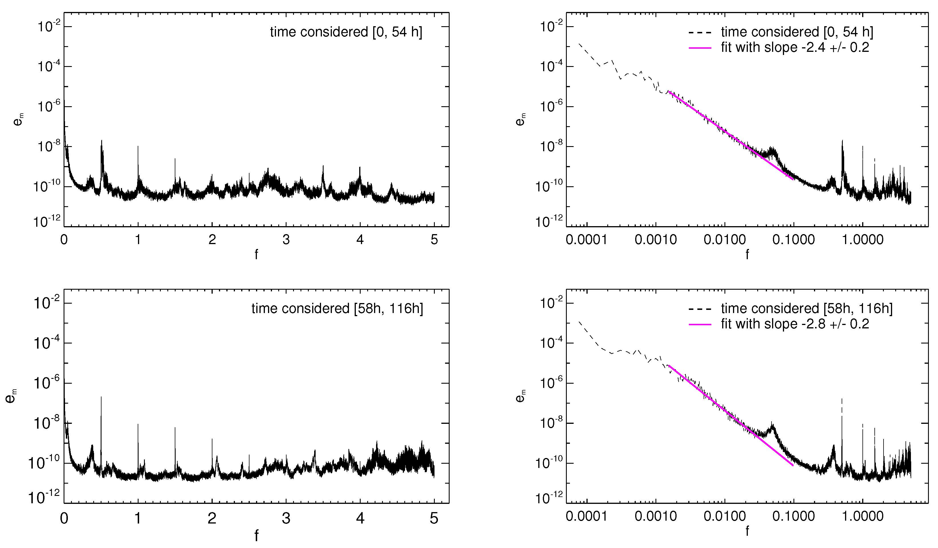
A relevant feature of kinetic and magnetic frequency spectra is the existence of power-law ranges at low frequencies. Considering the kinetic spectrum, we find a power law dependence in the interval of frequencies [ 0 . 001 , 0 . 02 ] , corresponding to 6 . 6 × 10 5 Hz f 1 . 3 × 10 3 Hz, in physical units. A fitting procedure gives a spectral index b = 1 . 0 ± 0 . 2 when the spectrum is calculated in the time interval [ 0 h, 54 h]. The index value slightly increases in absolute value when the time series considered for computing the spectrum is in the interval [ 58 h, 116 h], though this variation remains within the error bar. The existence of a power-law ranges in spectra of velocity measured in corona has been pointed out by [9,10,11], in the frequency range 2 × 10 4 Hz f 10 2 Hz. The spectral index varies according to the considered region within the corona, but it is around b 1 in quiet-Sun regions [11]. Therefore, the power-law range found in our result is in good accordance with measures of velocity fluctuations in quiet-Sun regions.
Considering magnetic spectra (Figure 7), the power law is steeper and much more energy is accumulated mostly at low frequencies with respect to kinetic spectra. Moreover, the difference in the spectral index is significant (out of the error bar) when the spectrum is computed for the time series considered in time interval [ 0 h , 54 h ] ( b = 2 . 4 ± 0 . 2 ) and the time interval [ 58 h , 116 h ] ( b = 2 . 8 ± 0 . 2 ). This actually indicates that in the latter time interval, where the velocity fluctuation level is lower, nonlinear interactions are significantly less efficient than in the former. In conclusion, our results indicate that a higher level of velocity fluctuations corresponds to a lower level of fluctuating energy (mainly magnetic), a higher value of dissipation and a shallower magnetic spectrum. All these features are related with a larger spectral energy flux associated with the nonlinear cascade.
In Figure 8 the transverse kinetic and magnetic spectra, defined by ε v = | v n ( x , t ) | and ε b = | b n ( x , t ) | , respectively, are plotted as functions of the transverse wavenumber k n . Angular parentheses indicate space average in the domain 0 x 1 and time average over a given interval T. The left and right panel refer to the time intervals T 1 = [ 0 , 54 h ] and T 2 = [ 58 h , 116 h ] , respectively. At large transverse scales magnetic energy largely dominates over kinetic energy. However, there the magnetic spectrum is steeper and reaches the level of kinetic spectrum at intermediate wavenumbers, where a short range is present, with a kinetic-magnetic energy quasi-equipartition. The kinetic spectrum have a power-law range with a spectral index quite close to the Kolmogorov value (full line). Comparing the spectra in the two periods, we see that the of level of magnetic energy is larger in T 2 than in T 1 , consistently with larger total energy E (Figure 3); kinetic energy shows the opposite trend in the two periods.

4. Conclusions

In this paper we have presented a numerical simulation describing the long-term behaviour of turbulence in a coronal loop, which is continuously solicited at its bases by photospheric motions. The simulation covers a time interval of few thousand hours, which is much longer than any involved dynamical time. The possibility of representing such a long interval of the time evolution with an acceptable computational effort is due to the employment of the Hybrid Shell Model [33]. On the other hand, in order to avoid exceedingly longer computational times, a smaller spectral width has been used than, for instance, in [38]. This has given a less detailed description of the perpendicular kinetic and magnetic spectra. An important feature of the model is the possibility to implement boundary conditions at the loop bases, which represent a key aspect of the present work. In contrast, no boundary conditions can be specified in other kinds of shell models [30] which have been applied to represent the turbulence dynamics in the solar corona [31].
With respect to previous works [33,34,35], the present simulation includes a more realistic representation of plasma motion soliciting the loop. In particular, we have considered frequency spectra of photospheric motions, calculated at different spatial scales from a dataset of the SOHO/MDI instrument [12,13]. Such spectra show two different contributions: a peak at frequency ( 300 s ) 1 , corresponding to global p-mode oscillations, and a continuum at lower frequencies. The latter can be interpreted as due to the interaction between global gravity modes and the velocity pattern associated with convection. Indeed, numerical simulations have shown that the presence of the convective layer allows gravity modes, otherwise vanishing, to reach the photosphere and to appear as low-frequency oscillations at a spatial scale comparable with that of convection [52]. The relative contribution of p-modes and of low-frequency continuum is different at the various spatial scales.
In our model we have set up boundary conditions which emulate the above properties of photospheric motions. We have built up a numerical procedure which generates random motions at the loop bases at three different spatial scales. The associated velocity has multiple-Lorentzian spectra, whose parameters have been chosen in a way to fit the observed photospheric spectra. Such boundary conditions allow energy to enter the loop at different spatial and temporal scales, though the incoming power is determined by the interplay between boundary motions and internal dynamics [38,39]. For the considered parameters, we have found a net average incoming power P t 5 . 60 × 10 23 erg s 1 , corresponding to a incoming energy flux Φ i n = P t / L 2 5 . 6 × 10 5 erg s 1 cm 2 . Such a value compares well with the energy flux required to keep the quiet-Sun corona at the observed temperature against radiative and conductive losses [51]. In the model we have assumed that the spectral properties of photospheric motions can be directly used to define boundary conditions at the loop bases. This assumption neglects the presence of the chromosphere and of the transition region, located between the photosphere and the corona. Those strongly inhomogeneous layers can affect the transmission of motions from the photosphere to the corona; modelling in a realistic way their effects represents a difficult task, even if steps in that direction have been done (e.g., [54,55]). On the other hand, one can expect that motions at the coronal base are somehow related to motions in the photosphere. In this line of ideas, our model represents a step toward increasing realism with respect to a series of previous similar models [33,34,35,36,37,38,39], always bearing in mind its own limitations. In particular, the above estimation of the incoming energy flux Φ i n could be affected by the lack of the atmospheric layers between the photosphere and the corona.
Concerning the boundary condition, it might be interesting to compare the dynamics here described with that obtained using “open” boundary conditions, which have been considered in another model [55] based on the same equations as the hybrid shell model. In open boundary conditions the incoming Elsässer variable is specified at boundaries, instead of velocity. In that model is has been found that an energy leakage is present for open boundary conditions, which modifies the dynamics, e.g., sensibly lowering the level of turbulent fluctuations [55]. In our case, the choice of imposing the velocity at the boundaries (“line-tying” boundary conditions) is based on the consideration that, due to the much larger density of lower atmospheric layers, the inertia of the fluid underlying the corona is much higher than that of the coronal plasma. As a consequence, the velocity in low layers drives motions at the coronal base. We also notice that a certain level of energy leakage is also present in our model. In fact, we have found an amount of outcoming power which is of the same order as the incoming power (Figure 3).
The fluctuating energy inside the loop is mainly magnetic, indicating that frequencies lower than t A 1 are mainly responsible for the loop energization, similar to what happens in classical DC heating mechanims. However, though the kinetic energy level is much lower than magnetic energy, velocity fluctuations play an important role in controlling the turbulent cascade, and consequently dissipation and heating. In fact, in our simulation we observed that a higher level of velocity fluctuations corresponds to a larger dissipated power and a lower level of fluctuating energy. This is in accordance with previous numerical results [34], as well as analytical predictions [38,39] showing that the energy flux along the spectrum is larger for higher levels of fluctuating velocity. Therefore, in our model both DC and AC phenomena are important: while DC phenomena seem to regulate the net energy input and determine the predominance of magnetic with respect to kinetic energy, AC phenomena regulate the energy flux along the spectrum and, indirectly, dissipation and heating. The model results indicate a time-averaged velocity fluctation inside the loop ranging between ∼45 and ∼60 km/s. These values are of the order of typical fluctuating velocities of coronal plasma deduced from measures of nonthermal broadenings of coronal lines [14].
The fluctuating velocity inside the loop is one order of magnitude larger that the velocity imposed at the loop bases. This growth of velocity amplitude in the loop body indicates kinetic energy storage, due to a resonance effect. The phenomenon of loop resonance is confirmed by the presence of well-defined resonance lines in the higher frequency part of both kinetic and magnetic energy spectra. A signature of the peak at frequency f 3 . 3 × 10 2 Hz in the spectrum of boundary condition is found both in the kinetic and magnetic spectrum. Another relevant feature is localized in the lower frequency part of the kinetic energy spectrum, namely, a power-law range, with spectral index 1 in the frequency range 6 . 6 × 10 5 Hz f 1 . 3 × 10 3 Hz. It compares well with frequency spectra of velocity measured in coronal structures [9,11]. Indeed, in such spectra power-law ranges are found for 2 × 10 4 Hz f 10 2 Hz, with a spectral index which is 1 in quiet-Sun regions [11]. Magnetic reconnection in complex magnetic configurations, like in the quiet-Sun corona, has been considered as an additional source of Alfvén waves [56]. However, magnetic reconnection cannot be described by our model, due to the lack of spatial dependence on transverse coordinates.
In conclusion, our numerical model, with the implementation of more realistic boundary conditions, is able to reproduce several observational features of coronal structures in quiet-Sun regions, with particular regard to velocity spectra. In the next future we plan to improve the realism of the model by including a longitudinal stratification of the density, in order to reproduce possible effects of gravity, such as partial reflection of parallel-propagating perturbations.

Author Contributions

Data curation, F.M., A.V. and F.D.M.; Investigation, G.N.; Methodology, G.N., F.M., V.C. and P.V.; Software, G.N., L.P. and V.C.; Writing—original draft, G.N. and F.M. All authors have read and agreed to the published version of the manuscript.

Funding

This research received no external funding.

Conflicts of Interest

The authors declare no conflict of interest.

References

  1. Parker, E.N. Hydromagnetic Dynamo Models. Astrophys. J. 1955, 122, 294–314. [Google Scholar] [CrossRef]
  2. Pongkitiwanichakul, P.; Nigro, G.; Cattaneo, F.; Tobias, S.M. Shear-driven Dynamo Waves in the Fully Nonlinear Regime. Astrophys. J. 2016, 825, 23. [Google Scholar] [CrossRef] [Green Version]
  3. Nigro, G.; Pongkitiwanichakul, P.; Cattaneo, F.; Tobias, S.M. What is a large-scale dynamo? Mon. Not. R. Astron. Soc. 2017, 464, L119–L123. [Google Scholar] [CrossRef]
  4. Nigro, G. Attracted by the fascinating magnetism of the Sun. Il Nuovo Cimento C 2019, 42, 1. [Google Scholar]
  5. Nigro, G.; Carbone, V.; Primavera, L. Simplified model for an α2-ω dynamo fed by dynamical evolution of the zonal shear. Mon. Not. R. Astron. Soc. 2013, 433, 2206–2214. [Google Scholar] [CrossRef] [Green Version]
  6. Nigro, G. A shell model for a large-scale turbulent dynamo. Geophys. Astrophys. Fluid Dyn. 2013, 107, 101–112. [Google Scholar] [CrossRef]
  7. Nigro, G.; Veltri, P. A Study of the Dynamo Transition in a Self-consistent Nonlinear Dynamo Model. Astrophys. J. Lett. 2011, 740, L37. [Google Scholar] [CrossRef] [Green Version]
  8. Vecchio, A.; Cauzzi, G.; Reardon, K.P.; Janssen, K.; Rimmele, T. Solar atmospheric oscillations and the chromospheric magnetic topology. Astron. Astrophys. 2007, 461, L1–L4. [Google Scholar] [CrossRef] [Green Version]
  9. Tomczyk, S.; McIntosh, S.W. Time-Distance Seismology of the Solar Corona with CoMP. Astrophys. J. 2009, 697, 1384–1391. [Google Scholar] [CrossRef] [Green Version]
  10. McIntosh, S.W.; De Pontieu, B.; Carlsson, M.; Hansteen, V.; Boerner, P.; Goossens, M. Alfvénic waves with sufficient energy to power the quiet solar corona and fast solar wind. Nature 2011, 475, 477–480. [Google Scholar] [CrossRef]
  11. Morton, R.J.; Tomczyk, S.; Pinto, R.F. A global view of velocity fluctuations in the corona below 1.3 R with CoMP. Astrophys. J. 2016, 828, 89. [Google Scholar] [CrossRef] [Green Version]
  12. Vecchio, A.; Carbone, V.; Lepreti, F.; Primavera, L.; Sorriso-Valvo, L.; Veltri, P.; Alfonsi, G.; Straus, T. Proper Orthogonal Decomposition of Solar Photospheric Motions. Phys. Rev. Lett. 2005, 95, 061102. [Google Scholar] [CrossRef] [PubMed]
  13. Vecchio, A.; Carbone, V.; Lepreti, F.; Primavera, L.; Sorriso-Valvo, L.; Straus, T.; Veltri, P. Spatio-Temporal Analysis of Photospheric Turbulent Velocity Fields Using the Proper Orthogonal Decomposition. Sol. Phys. 2008, 251, 163–178. [Google Scholar] [CrossRef]
  14. Chae, J.; Schühle, U.; Lemaire, P. SUMER measurements of nonthermal motions: Constraints on coronal heating mechanisms. Astrophys. J. 1998, 505, 957. [Google Scholar] [CrossRef]
  15. Milano, L.; Gomez, D.O.; Martens, P.C.H. Solar Coronal Heating: AC versus DC. Astrophys. J. 1997, 490, 442–451. [Google Scholar] [CrossRef] [Green Version]
  16. Heyvaerts, J.; Priest, E.R. Coronal heating by phase-mixed shear Alfven waves. Astron. Astrophys. 1983, 117, 220–234. [Google Scholar]
  17. Similon, P.L.; Sudan, R.N. Energy Dissipation of Alfven Wave Packets Deformed by Irregular Magnetic Fields in Solar-Coronal Arches. Astrophys. J. 1989, 336, 442–453. [Google Scholar] [CrossRef]
  18. Califano, F.; Chiuderi, C.; Einaudi, G. Nonresonant Resistive Dissipation of Incompressible Magnetohydrodynamic Waves. Astrophys. J. 1990, 365, 757–763. [Google Scholar] [CrossRef]
  19. Malara, F.; Veltri, P.C.; hiuderi, C.; Einaudi, G. Incompressible disturbances in nonuniform media: Formation of small scales. Astrophys. J. 1992, 396, 297–310. [Google Scholar] [CrossRef]
  20. Malara, F.; Primavera, L.; Veltri, P. Formation of small scales via Alfvén wave propagation in compressible nonuniform media. Astrophys. J. 1996, 459, 347–364. [Google Scholar] [CrossRef]
  21. Petkaki, P.; Malara, F.; Veltri, P. Topological formation of small scales in magnetohydrodynamics: A fast dissipation mechanism. Astrophys. J. 1998, 500, 483–491. [Google Scholar] [CrossRef]
  22. Malara, F.; Petkaki, P.; Veltri, P. Dissipation of Alfvén waves in force-free magnetic fields: Competition between phase mixing and three-dimensional effects. Astrophys. J. 2000, 533, 523–534. [Google Scholar]
  23. Malara, F.; De Franceschis, M.F.; Veltri, P. Alfvén wave propagation and dissipation in a 3D-structured compressible plasma. Astron. Astrophys. 2003, 412, 529–539. [Google Scholar] [CrossRef]
  24. Malara, F.; De Franceschis, M.F.; Veltri, P. Dissipation of Alfvén wave in complex 3D coronal force-free structures. Astron. Astrophys. 2005, 443, 1033–1046. [Google Scholar] [CrossRef]
  25. Malara, F.; De Franceschis, M.F.; Veltri, P. Alfvén wave dissipation and topological properties of 3D coronal force-free magnetic fields. Astron. Astrophys. 2007, 467, 1275–1284. [Google Scholar] [CrossRef] [Green Version]
  26. Pucci, F.; Onofri, M.; Malara, F. Evolution of magnetohydrodynamic waves in low layers of a coronal hole. Astrophys. J. 2014, 796, 43. [Google Scholar] [CrossRef] [Green Version]
  27. Vásconez, C.L.; Pucci, F.; Valentini, F.; Servidio, S.; Matthaeus, W.H.; Malara, F. Kinetic Alfvén wave generation by large-scale phase mixing. Astrophys. J. 2015, 815, 7. [Google Scholar] [CrossRef] [Green Version]
  28. Pucci, F.; Vásconez, C.L.; Pezzi, O.; Servidio, S.; Valentini, F.; Matthaeus, W.H.; Malara, F. From Alfvén waves to kinetic Alfvén waves in an inhomogeneous equilibrium structure. J. Geophys. Res. Space Phys. 2016, 121, 1024–1045. [Google Scholar] [CrossRef] [Green Version]
  29. Einaudi, G.; Velli, M.; Politano, H.; Pouquet, A. Energy Release in a Turbulent Corona. Astrophys. J. 1996, 457, L113–L116. [Google Scholar] [CrossRef]
  30. Giuliani, P.; Carbone, V. A note on shell models for MHD turbulence. Europhys. Lett. 1998, 43, 527–532. [Google Scholar] [CrossRef] [Green Version]
  31. Boffetta, G.; Carbone, V.; Giuliani, P.; Veltri, P.; Vulpiani, A. Power Laws in Solar Flares: Self-Organized Criticality or Turbulence? Phys. Rev. Lett. 1999, 83, 4662–4665. [Google Scholar] [CrossRef] [Green Version]
  32. Dmitruk, P.; Gómez, D.O. Scaling Law for the Heating of Solar Coronal Loops. Astrophys. J. 1999, 527, L63–L66. [Google Scholar] [CrossRef] [PubMed] [Green Version]
  33. Nigro, G.; Malara, F.; Carbone, V.; Veltri, P. Nanoflares and MHD Turbulence in Coronal Loops: A Hybrid Shell Model. Phys. Rev. Lett. 2004, 92, 194501. [Google Scholar] [CrossRef] [PubMed]
  34. Nigro, G.; Malara, F.; Veltri, P. Large-Amplitude Velocity Fluctuations in Coronal Loops: Flare Drivers? Astrophys. J. 2005, 629, L133–L136. [Google Scholar] [CrossRef]
  35. Reale, F.; Nigro, G.; Malara, F.; Peres, G.; Veltri, P. Modeling a Coronal Loop Heated by Magnetohydrodynamic Turbulence Nanoflares. Astrophys. J. 2005, 633, 489–498. [Google Scholar] [CrossRef]
  36. Veltri, P.; Nigro, G.; Malara, F.; Carbone, V.; Mangeney, A. Intermittency in MHD turbulence and coronal nanoflares modelling. Nonlin. Proc. Geophys. 2005, 12, 245–255. [Google Scholar] [CrossRef] [Green Version]
  37. Buchlin, E.; Velli, M. Shell Models of RMHD Turbulence and the Heating of Solar Coronal Loops. Astrophys. J. 2007, 662, 701–714. [Google Scholar] [CrossRef] [Green Version]
  38. Nigro, G.; Malara, F.; Veltri, P. Resonant behavior and fluctuating energy storage in coronal loops. Astrophys. J. 2008, 685, 606–621. [Google Scholar] [CrossRef]
  39. Malara, F.; Nigro, G.; Onofri, M.; Veltri, P. Fluctuating energy storage and nonlinear cascade in an inhomogeneous coronal loop. Astrophys. J. 2010, 720, 306–327. [Google Scholar] [CrossRef]
  40. Rappazzo, A.F.; Velli, M.; Einaudi, G.; Dahlburg, R.B. Coronal heating, weak MHD turbulence, and scaling laws. Astrophys. J. 2007, 657, L47–L51. [Google Scholar] [CrossRef] [Green Version]
  41. Rappazzo, A.F.; Velli, M.; Einaudi, G.; Dahlburg, R.B. Nonlinear dynamics of the Parker scenario for coronal heating. Astrophys. J. 2008, 677, 1348–1366. [Google Scholar] [CrossRef] [Green Version]
  42. Rappazzo, A.F.; Velli, M. Magnetohydrodynamic turbulent cascade of coronal loop magnetic fields. Phys. Rev. E 2011, 83, 065401. [Google Scholar] [CrossRef] [PubMed] [Green Version]
  43. Magyar, N.; Van Doorsselaere, T.; Goossens, M. Understanding Uniturbulence: Self-cascade of MHD waves in the presence of inhomogeneities. Astrophys. J. 2019, 882, 50. [Google Scholar] [CrossRef] [Green Version]
  44. Pontin, D.I.; Hornig, G. The structure of current layers and degree of field-line braiding in coronal loops. Astrophys. J. 2015, 805, 47. [Google Scholar] [CrossRef]
  45. De Moortel, I.; Pascoe, D.J.; Wright, A.N.; Hood, A.W. Transverse, propagating velocity perturbations in solar coronal loops. Plasma Phys. Control. Fusion 2016, 58, 014001. [Google Scholar] [CrossRef] [Green Version]
  46. Karampelas, K.; Van Doorsselaere, T.; Antolin, P. Heating by transverse waves in simulated coronal loops. Astron. Astrophys. 2017, 604, A130. [Google Scholar] [CrossRef] [Green Version]
  47. Mingzhe, G.; Van Doorsselaere, T.; Karampelas, K.; Li, B.; Antolin, P.; De Moortel, I. Heating Effects from Driven Transverse and Alfvén Waves in Coronal Loops. Astrophys. J. 2019, 870, 55. [Google Scholar]
  48. Nigro, G.; Carbone, V. Finite-time singularities and flow regularization in a hydromagnetic shell model at extreme magnetic Prandtl numbers. New J. Phys. 2015, 17, 073038. [Google Scholar] [CrossRef] [Green Version]
  49. Strauss, H. Nonlinear, three-dimensional magnetohydrodynamics of noncircular tokamaks. Phys. Fluids 1976, 19, 134. [Google Scholar] [CrossRef]
  50. Zank, G.P.; Matthaeus, W.H. Nearly incompressible fluids. II: Magnetohydrodynamics, turbulence, and waves. Phys. Fluids A 1993, 5, 257. [Google Scholar] [CrossRef]
  51. Withbroe, G.L. The temperature structure, mass, and energy flow in the Corona and inner Solar Wind. Astrophys. J. 1988, 325, 442–467. [Google Scholar] [CrossRef]
  52. Onofri, M.; Vecchio, A.; De Masi, G.; Veltri, P. Propagation of gravity waves in a convective layer. Astrophys. J. 2012, 746, 58. [Google Scholar] [CrossRef] [Green Version]
  53. Cadavid, A.C.; Lawrence, J.K.; Christian, D.J.; Jess, D.B.; Nigro, G. Heating Mechanisms for Intermittent Loops in Active Region Cores from AIA/SDO EUV Observations. Astrophys. J. 2014, 795, 48. [Google Scholar] [CrossRef] [Green Version]
  54. van Ballegooijen, A.A.; Asgari-Targhi, M.; Cranmer, S.R.; DeLuca, E.E. Heating of the solar chromosphere and corona by Alfvén wave turbulence. Astrophys. J. 2011, 736, 3. [Google Scholar] [CrossRef] [Green Version]
  55. Verdini, A.; Grappin, R.; Velli, M. Coronal heating in coupled photosphere-chromosphere-coronal systems: Turbulence and leakage. Astron. Astrophys. 2012, 538, A70. [Google Scholar] [CrossRef] [Green Version]
  56. Cranmer, S.R. Low-frequency Alfvén Waves Produced by Magnetic Reconnection in the Sun’s Magnetic Carpet. Astrophys. J. 2018, 862, 6. [Google Scholar] [CrossRef]
Figure 1. Upper panel: the spectra U 0 ( f ) (purple line) and F 0 ( 2 π f ) (dashed line); middle panel: the spectra U 1 ( f ) (green line) and F 1 ( 2 π f ) (dashed line); lower panel: the spectra U 2 ( f ) (light blue line) and F 2 ( 2 π f ) (dashed line). Each spectra is divided by the integrated energy U T and is plotted as a function of the normalized frequency f.
Atmosphere 11 00409 g001
Figure 2. Power spectrum of the velocity v imposed at the boundary x = 0 , as a function of the normalized frequency f.
Atmosphere 11 00409 g002
Figure 3. The total energy E (upper panel), the dissipated power W (middle panel) and the net incoming power P (lower panel) are plotted as functions of time t.
Atmosphere 11 00409 g003
Figure 4. The normalized cross helicity σ c = ( E + E ) / ( E + + E ) (upper panel) remains quite close to zero during the simulation time, except around t 280 h , while the mean-square magnetic potential H A = < n = 0 n m a x ( | b n | / k n ) 2 > x (lower panel) has the same profile of the total energy as functions of the time t.
Atmosphere 11 00409 g004
Figure 5. The RMS velocity v R M S (left panel) and magnetic field b R M S (right panel) fluctuations are plotted as functions of x for the whole simulation time (black solid lines), for the interval 0 t 54 h (grey dot-dashed lines) and for the interval 58 h t 116 h (magenta dashed lines).
Atmosphere 11 00409 g005
Figure 6. The kinetic spectra e v (black lines) vs. frequency f = ω / 2 π display resonance spikes and peaks, clearly detectable both in semi-log scale (left panels) and log scale (right panels), as well as a power-law range at low frequencies (the magenta line indicate a fitting in the frequency interval 0 . 001 < f < 0 . 1 ). The kinetic energy spectrum does not seem to significantly change when computed at diverse time intervals: 0 t 54 h (upper panels) and 58 h t 116 h (lower panels)).
Atmosphere 11 00409 g006
Figure 7. The magnetic spectra e b (black lines) plotted vs. frequency f = ω / 2 π display resonance spikes, broader peaks and a power-law range at low frequencies, clearly observable when plotted both in semi-log scale (left panels) and log scale (right panels). The power-law (magenta line) fitting the spectra in the frequency interval 0 . 001 < f < 0 . 1 changes index when calculated in the time intervals 0 t 54 h (upper panels) and 58 h t 116 h (lower panels), showing the accumulation of magnetic energy at large scales in the second time interval.
Atmosphere 11 00409 g007
Figure 8. The kinetic and magnetic energy spectrum vs. the transverse wavenumber k n (black triangles and magenta circles, respectively) computed by making the time average in T 1 = [0, 54 h] (left panel) and T 2 = [58 h, 116 h] (right panel). A function proportional to k n 2 / 3 is plotted for comparison (full line). Even though the energy values are depicted in the logarithmic scale, the increase of the magnetic energy in T 2 is appreciable compared to the values reached in T 1 . Kinetic energy has the opposite trend in these two periods.
Atmosphere 11 00409 g008
Table 1. Values of the parameters of the multiple Lorentzian spectrum.
Band a n , 0 T n , 0 1 a n , 1 T n , 1 1 ω n , 1 / ( 2 π ) N
B0 3 . 84 0 . 010 9 . 70 0 . 030 0 . 05 10 4
B1 6 . 21 0 . 015 6 . 58 0 . 030 0 . 05 10 4
B2 6 . 58 0 . 020 2 . 33 0 . 030 0 . 06 10 4

