Polarimetric Backscatter Sonde Observations of Southern Ocean Clouds and Aerosols

Abstract

Balloon-borne polarimetric backscatter sonde (polarsonde) observations of aerosol and cloud during the approach of a cold front at Macquarie Island (54.499 S 158.937 E) are described. The polarsonde captures vertical profiles of cloud occurrence and phase. The cloud base and cloud top heights from the backscatter sonde compare favourably with observations made by a co-located cloud radar and ceilometer. An estimate of the total scatter probability from a liquid cloud layer at 1000 m height is used with a Monte Carlo model of the instrument to obtain cloud particle concentration, and this is compared to a measurement of cloud condensation nucleus concentration made at sea level. Backscatter from aerosol, as well as cloud, is significant. A high aerosol loading in part of the pre-frontal airmass is observed at altitudes up to 6 km. Below the melting level, the high cross-polarised return, relative to the co-polarised, indicates a substantial concentration of solid, non-spherical aerosol particles, which due to the high humidity cannot be sea salt or sulphate. A back trajectory analysis indicates that the observed aerosol includes continental dust.

1. Introduction

It has been recognised for some time that the cloudiness of the Southern Ocean (45${}^{°}$ S to 60${}^{°}$ S) is poorly captured in climate models [1,2]. The predicted amount of cloud over this region is generally too low, though this is not unique to this part of the world. More dramatic is that models predict much more ice at the cloud top over the Southern Ocean than is observed by satellites [3]. These discrepancies have major implications for modelling of the earth’s radiation budget and weather because the albedo of clouds is dependent on the shapes of the cloud particles [4]. Closely connected to the cloudiness are the generation, transport and evolution of aerosols in the atmosphere because aerosols are the nucleation sites for cloud droplet formation and initiation of freezing. It has been suggested that the increased frequency of super-cooled liquid in Southern Ocean clouds is at least in part due to lower aerosol (and ice nuclei) loadings in the southern hemisphere [5].

The Southern Ocean is often considered as a “pristine” region (e.g., [6,7]), where aerosols are purely natural, having no anthropogenic component, or that they are mainly of marine origin and have no continental source (e.g., dust or smoke). Measuring aerosols in pristine environments is important for providing a baseline for resolving uncertainties in the impact of anthropogenic aerosols on cloud albedo and the earth’s radiation budget [8], as well as their direct radiative effects, though continental aerosols do sometimes intrude into this region [9]. The structure of the marine boundary layer will also affect the vertical distribution of aerosols so that measurements of the aerosol distribution serve as a probe for unmixed layers within the boundary layer. Sulphate aerosol is a major component of concentrations of total aerosol (CCN) [10], and vertical profiles of aerosols could be useful in elucidating pathways for oxidation of biogenic dimethyl sulphide to sulphate [7,11].

An increasing number of aircraft and surface-based measurement campaigns in the Southern Ocean has taken place in the last few years; for example, “High-performance Instrumented Airborne Platform for Environmental Research Pole-to-Pole Observations” [12], “Clouds, Aerosols, Precipitation, Radiation, and Atmospheric Composition over the Southern Ocean project” [13,14], “Measurements of Aerosols, Radiation, and Clouds over the Southern Ocean” [15,16], “The Southern Ocean Clouds, Radiation, Aerosol Transport Experimental Study” [17] and the “Atmospheric Tomography Mission” [18]. These have included passive sensing (e.g., radiometers), active sensing (lidars and radars) and, on the airborne platforms, particle imaging probes. A further important source of data on clouds and aerosols is satellites; Cloudsat and CALIPSO carry radar and lidar instruments, respectively, and over our region of interest for this paper is the Himawari8 geostationary satellite of the Japanese Meteorological Agency, with infrared and visible imagers.

Measurements of aerosols and the thermodynamic phase of cloud particles over the Southern Ocean are problematic for several reasons. Surface-based and aircraft campaigns are expensive, and measurements are sparse because of the severe weather and oceanic nature of the region. Most measurements in the region are made by satellite, which can provide much wider geographical coverage than a campaign, which is restricted to a ship or aircraft track or a fixed point on the surface. However, a limitation of satellite observations is that the measurements have a low sampling rate over a particular location if the satellites are not geostationary, or otherwise have low horizontal resolution. An additional issue arises because much of the cloud is very low-level (500–1000 m) [19], which satellites have difficulty observing [4,20].

For producing a vertical profile of aerosol concentration and cloud density and phase, each type of sensor has different limitations and advantages: lidar tends to have difficulty seeing past the proximal edge of thick clouds due to attenuation and multiple scatter (but does see scatter from both cloud and aerosol); radar typically has lower range resolution and does not scatter from aerosol (but suffers less from attenuation); radiometers have low range resolution (but are simple and robust); and imaging devices, being in-situ sensors, need a vertically moving platform (but resolve different ice-crystal habits in clouds). Thus, as no one of these devices is ideal, these methods complement each other.

In addition to satellites and the campaign platforms, regular balloon soundings take place at several locations around the boundaries of the Southern Ocean, and at a few within the region. These measurements have been restricted to pressure, temperature and humidity, with a few of the soundings also measuring ozone concentrations. In this paper, we will describe results from a new in-situ sensor, a balloon-borne polarimetric backscatter sonde that was used to obtain profiles of clouds at Macquarie Island Research Station (54.499 S, 158.937 E) in the middle of the Southern Ocean. This instrument was conceived for the purpose of distinguishing super-cooled liquid water from ice particles in clouds, initially with a focus on aviation safety [21]. When carried by a weather balloon, using a radiosonde for telemetry (as well as temperature and humidity measurements), it provides a profile of the backscattering particles from the ground to the lower stratosphere. In the event, it also detects aerosols as they have backscattering that is greater relative to the forward scattering than larger cloud particles with a larger overall scattering cross section. Note that in this paper we use the term “backscatter” loosely, as the scattering angles in question are in the range 160${}^{°}$ to 175${}^{°}$, rather than 180${}^{°}$ corresponding to exact backscattering.

The three profiles described here were taken during the approach of a cold front over Macquarie Island, where weather balloons are launched twice daily by the Australian Bureau of Meteorology. Although layers of supercooled liquid cloud particles are identified in these profiles, the discussion will be primarily about cloud and aerosol below the melting level because the separation of the signals from cloud and from the smaller aerosol particles has less ambiguity, and the calibration of the polarsonde enables a determination of liquid cloud particle concentration, based on an assumption about the particle size range. In the following sections, we will give a description of the backscatter sonde before presenting the profiles. The resulting cloud base height and cloud top height will be compared to cloud radar and ceilometer measurements. Then we will discuss a back trajectory analysis that helps to shed light on the nature of the aerosols.

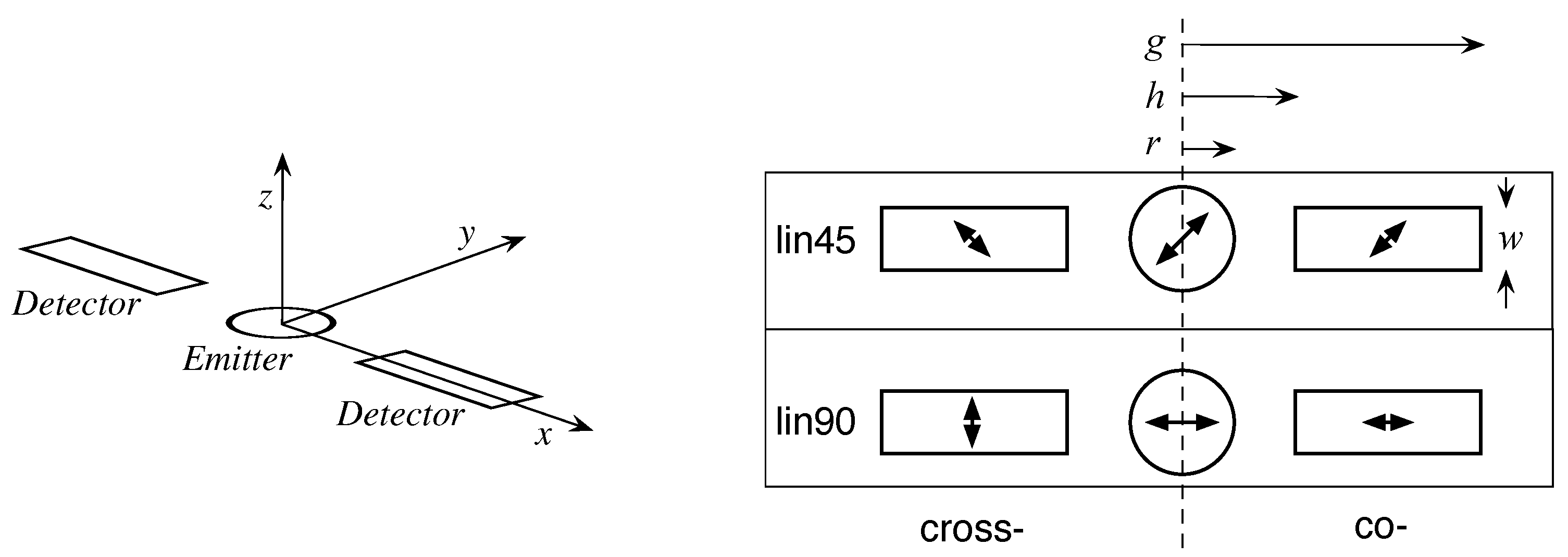
2. Polarsonde

The polarimetric backscatter sonde (“polarsonde” for short) was built to make an in-situ determination of whether the scattering particles in a cloud are spherical liquid droplets (possibly supercooled) or non-spherical ice particles. To first order, if the scattering angle is close to 180${}^{°}$ the spherical scatterers do not change the polarisation orientation of the scattered light, whereas nonspherical particles introduce substantial changes to the polarisation, and this depends on the shape of these particles. This picture is modified somewhat by the consideration of multiple scattering and reduction of the scattering angle to near backscattering directions.

The polarsonde emits polarised light from a pulsed LED into the atmosphere and detects light scattered near to the backscattering direction by particles at various distances, with detectors that have analyser polarisers. The polarsonde is a dual channel instrument, as illustrated in Figure 1. The LEDs and photodiodes (detectors) are surface mount devices attached to a printed circuit board. The LEDs are collimated by plastic catadioptric collimators glued on to the board over the LEDs, which project about 20 mm above the board. The polarisers for both the LED collimators and the detectors are polaroid films that were glued on with a thin layer of clear silicone sealant. The dimensions shown in Figure 1 are g = 70 mm, h = 45 mm, r = 10 mm and w = 4 mm.

In terms of Figure 1, the $x,z$–plane for each channel is approximately the scattering plane for detected photons from single scattering events. One channel has the emitted light polarised perpendicular, and the other at 45${}^{°}$, to the scattering plane. The channels are labelled “lin90” and “lin45”, respectively. There are two detectors for each channel, and they have polarisation axes oriented parallel (co-polarisation) and orthogonal (cross-polarisation) to the polarisation direction of the emitted light. The detectors in one channel are decoupled from the emitter of the other by time division multiplexing, as detailed below. In this work, only linear polarisation was used, though circular polarisation can also be used.

As is typical with polarimetric lidar work, the ratio of cross- to co-polarised signal is termed the depolarisation. If the signals (photocurrents) of the lin90 co- and cross-polarised detectors are denoted $I_{90}^{co}$ and $I_{90}^{cross}$, and similarly we have $I_{45}^{co}$ and $I_{45}^{cross}$, then the depolarisations for each channel are ${\delta }_{90}=I_{90}^{cross}/I_{90}^{co}$ and ${\delta }_{45}=I_{45}^{cross}/I_{45}^{co}$, respectively.

A Monte-Carlo model of the operation of the polarsonde [22], using the scattering matrices for a wide variety of randomly oriented ice crystal habits [23] and spheres (via Mie theory), indicates that for the lin90 polarisation, the simple picture of little depolarisation for spherical scatterers and substantial depolarisation for non-spherical scatterers is broadly correct, even when there is multiple scattering present. However, for the lin45 configuration, ${\delta }_{45}>1$ for spherical scatterers; this is in contrast to the lin90 configuration because the plane of polarisation of the emitted light is a plane of symmetry for the scattered light distribution, and in the lin45 configuration, the detectors are placed away from that plane, rather than in that plane as for lin90 [22].

Thus, for the purpose of distinguishing ice from liquid water, ${\delta }_{90}\simeq 0$ and ${\delta }_{45}>1$ for spherical liquid droplets, and ${\delta }_{90}\simeq 0.5$ and ${\delta }_{45}\simeq 0.5$, for ice. The reason that we have both channels is that if there are large (≃100 $\mathsf{\mu }$m) randomly oriented ice crystals with plate-like habit, the model showed that ${\delta }_{90}\simeq 0.1$, which could be interpreted as spheres because multiple scattering and scattering angles mean that for spheres ${\delta }_{90}\simeq 0$ is still an idealisation [22]. In essence, this is because the dominant scattering mechanism from the large plates is specular reflection from the basal facets. As we will see below, measurement noise is also a factor that makes ${\delta }_{90}\simeq 0.1$ interpretable as either spheres or large plates. Temperature measurement can resolve the ambiguity if T > 0 C. However, for large plate-like crystals ${\delta }_{45}\simeq 0.5$ which is relatively easy to distinguish from ${\delta }_{45}>1$ for spheres. As a general rule though, complication of the surface of an ice particle, such as by aggregation of smaller particles or roughening, sees both ${\delta }_{90}\simeq 0.5$ and ${\delta }_{45}\simeq 0.5$. For non-spherical particles smaller than 2 $\mathsf{\mu }$m, we do not have scattering matrix data or calculations available to apply the model, but as noted below, the model has been extended to such small spheres.

The LEDs for each polarisation channel are pulsed at 10 kHz (duty cycle of 50%) so that phase sensitive detection of the scattering signal can be used to separate the components of the detector photocurrent due to scattering of the LED light (wavelength 470 nm) and those due to other sources of light. To decouple the polarisation channels, they are switched on alternately, each for about 100 ms, so that the two can share a common microcontroller that performs analogue-to-digital conversion and implements the phase sensitive detection. This microcontroller also is set up with two data output formats; one is a standard serial interface, and the other is an interface to the external sensor input of a Vaisala RS92SGP radiosonde. The polarsondes were manufactured by Atrad Pty Ltd. in a batch of 30 identically constructed instruments, except in that in some the lin45 polarisers were substituted with circular polarisers (which were not used in the work reported here).

When flown with a weather balloon, a radiosonde is attached to the polarsonde to provide telemetry as well as pressure, temperature and humidity measurements. Measurements are reported once per second (set by the radiosonde), though there is a running time average performed by the microcontroller with an averaging time of 4 s. With a nominal balloon ascent rate of 5 m/s, this provides a vertical resolution of 20 m. A check of the background signal levels needs to be made before each flight; the procedure for this is described in Appendix A. The issue of possible riming of the instrument is considered in Appendix B.

Various calibrations (including the relative sensitivity of the detectors in each polarisation channel) and background signal measurements were made, as detailed in Appendix C. These calibrations were made on all polarsondes, and the variance in the ratio of sensitivities of the two detectors (with polaroids attached) over the set of instruments was around 5%. An additional calibration performed on some polarsondes is a measurement of the backscatter detection efficiency using a roughened PTFE sheet as a target. This was not performed on the actual polarsondes flown in this study, rather it was performed subsequently on identically constructed instruments. The method for this is described in Appendix C.

3. Description of Polarsonde Profiles

Here, we present data from three polarsonde flights, flown with weather balloons on 15/16 February 2017 at Macquarie Island. On that day, a cold front passed over the island at approximately 0200 UTC 16th February. The synoptic situation close to that time is shown in Figure 2. The polarsondes were launched at intervals of about three hours, with the first at 2020 UTC on the 15th. In all three launches, the balloon ascent rate was 4.2 m/s, though it did vary a little during the ascent.

The backscatter profiles for the first launch, in prefrontal conditions, are shown in Figure 3. The profiles for the lin90 the lin45 polarisation channels are shown separately in Figure 3a,c. Although the signals for backscatter are shown with arbitrary units (a.u.), the scaling of the raw signal voltages is identical in Figure 3a,c. The temperature and humidity profiles recorded by the accompanying radiosonde (Vaisala RS92SGP) are shown also. In one graph, the humidity is displayed as relative humidity, and in the other, as dew point temperature (generated by the Vaisala Digicora system), which is useful in establishing where cloud should be; i.e., when the temperature and the dewpoint are about the same. The melting level is at 2020 m. In Figure 3a,c for each detected signal, the inductive pickup background was subtracted, and a correction factor was applied to the cross-polarised trace to account for the different sensitivities of the co- and cross-polarised detectors, as detailed in Appendix C.

Both profiles show a broad, more or less smoothly varying, background up to about 6000 m. This is attributed mostly to aerosols. Below the melting level, any cloud would have spherical liquid water droplets and would not contribute significantly to the cross-polarised signal. On top of this background are enhancements of the signal, not necessarily for both co- and cross-polarised traces, that are attributed to cloud layers. The calibrated total backscatter for the lin90 channel in this launch is shown in Figure 4 , which is annotated with what we believe to be the total signal level for the background aerosol. The magnitude of the calibrated signal is discussed below in the context of what we can learn about the cloud particle concentration, and what we might expect from typical aerosol concentrations.

In Figure 3b,d the depolarisation for each channel is shown. This is calculated twice, once for the signal due to both cloud and aerosol (the red trace), which we denote ${\delta }_{90}^{raw}$ and ${\delta }_{45}^{raw}$, and then for the cloud below the melting level, denoted ${\delta }_{90}^{cloud}$ and ${\delta }_{45}^{cloud}$. The aerosol contribution is estimated for the co- and cross-polarised signals in the same way as shown in Figure 4 for the total backscattered signal. In calculating ${\delta }_{90,45}^{cloud}$, we only do this below the melting level, as we are much less confident in this estimation above the melting level. The aerosol contributions are subtracted from the signals, and the depolarisations for the cloud are calculated from the remainders. These are shown as black dots.

Various features in the profile are labelled and listed below. Those with capital letters are apparent layers of cloud, and those with lower case are other features. The features are present also in the lin45 graph, though with different apportioning of the signal between the co- and cross-polarised sub-channels. Some of the features appear also in the graphs of depolarisation.

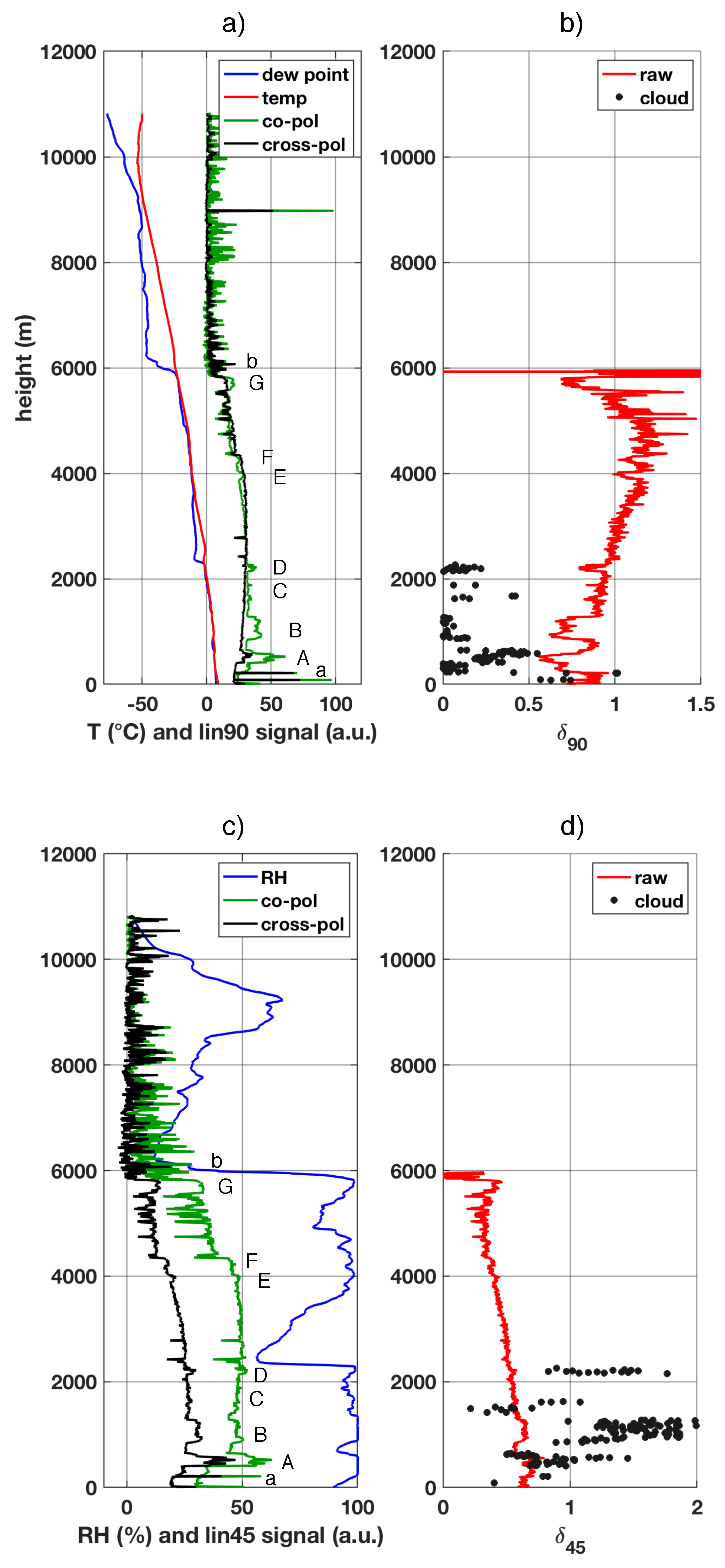
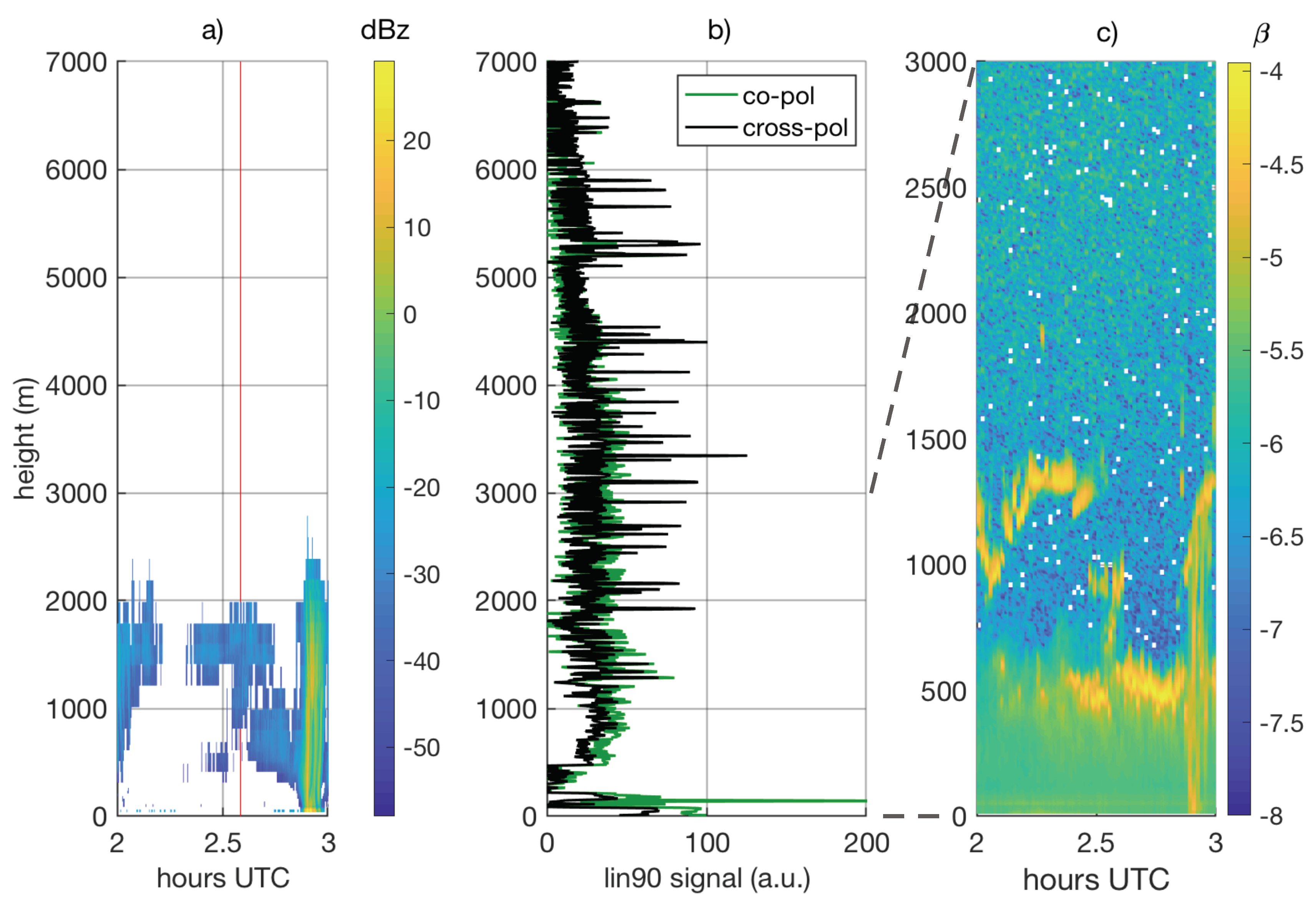
• a—there are three very sharp peaks in the polarsonde signal shortly after launch. These appear on both channels, though the second on the lin45 channel barely shows up. The first is likely due to the illumination of the ground or the balloon as the sonde package swings around on launch. The next two are attributed to the instrument passing through the exhaust plume from the station diesel power plant, which is wafting in the same general direction that the balloon takes, but with a slower ascent rate.
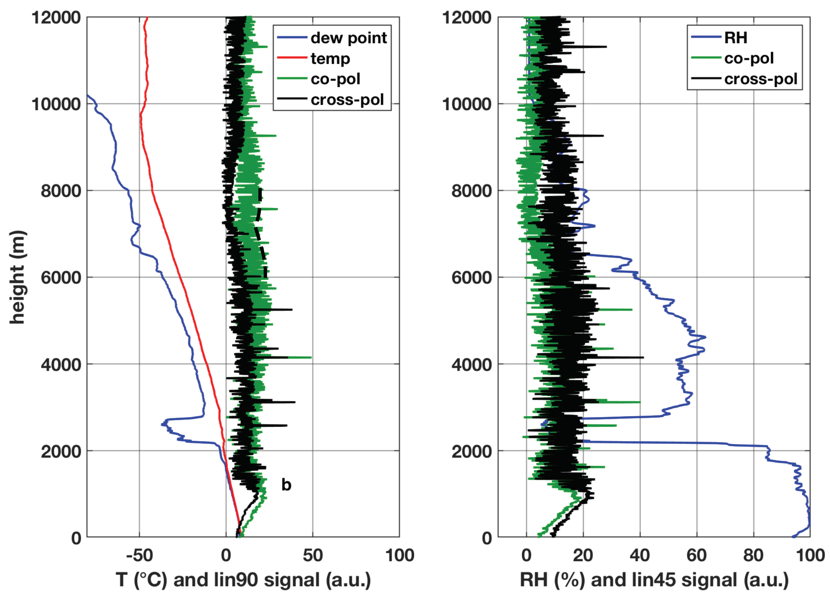
• b—at about 6000 m, the instrument emerges from the cloud top (of the top layer) into bright sunlight. As detailed in Appendix D, the sonde rotates below the balloon and it repeatedly points directly at the sun, and the extra resulting photocurrent leads to saturation of the preamplifier and thus gains compression of the modulated signal, leading to a “spikey” signal. While not desirable for detecting aerosol above the cloud, it does identify clearly the cloud top during the daytime.
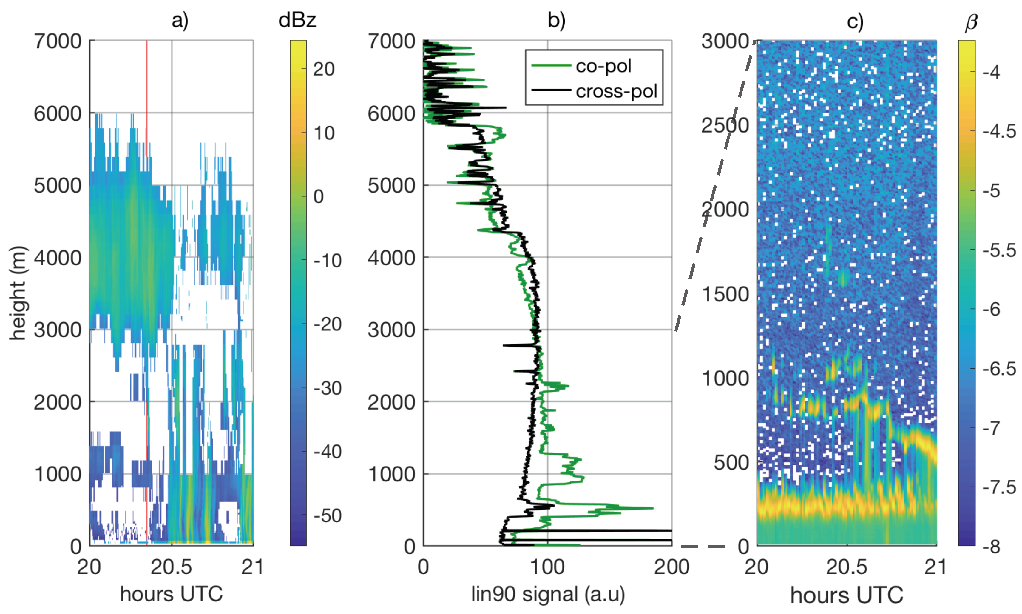
• A—the instrument passes through a layer of cloud some 500 m thick, which seems to be composed of two sub-layers. The lower of these seems to comprised of only liquid droplets, there being no associated rise in the cross-polarised signal for lin90. The second (upper) sublayer gives a stronger signal, but notably the cross-polarised signal for lin90 rises. This indicates that, in addition to the background aerosol, there is insoluble, nonspherical aerosol entrained in this sublayer, which is otherwise liquid water cloud. Because the lin90 cross-polarised signal rises a little and falls in concert with the co-polarised signal, we infer that the background is due to aerosol and is not an instrumental artefact. In the lower sublayer, the cloud depolarisation ${\delta }_{90}^{cloud}$ is less than 0.2, but in the upper sublayer, it is closer to 0.5. This also implies that there is solid material entrained in this layer. However, the cloud plus aerosol depolarisation ${\delta }_{90}^{raw}$ shows a very distinct dip even for the upper sublayer because the co-polarised signal rises more than the cross-polarised.
• B—a 500 m thick layer of cloud is encountered at about 1000 m height, but this layer is apparently only liquid water, with no insoluble particles entrained, because the cross-polarised lin90 signal shows no sign of this layer. Although there are apparently no aerosols entrained with this layer, the general background of aerosols is still present. Much of the discussion below centres on this layer. Note that with the background aerosol signal subtracted, ${\delta }_{90}^{cloud}\simeq 0$ and ${\delta }_{45}^{cloud}>1$ in agreement with the prediction of the Monte-Carlo model for spherical droplets.
• C—below 2000 m, a pair of thin liquid water layers appears. These show up also as small dips in ${\delta }_{90}^{total}$.
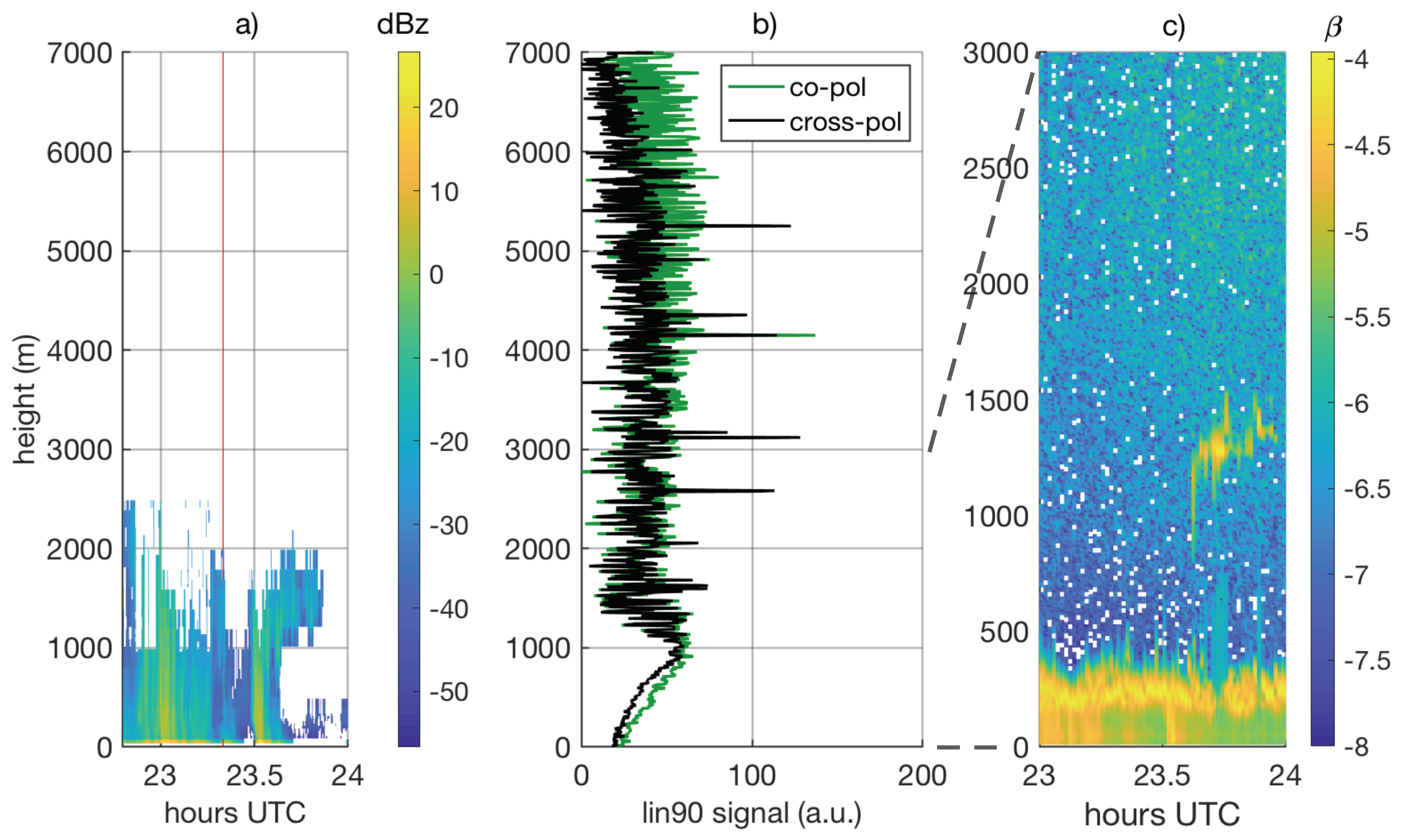
• D—a more substantial layer of liquid water cloud appears at about 2200 m. In the graph of ${\delta }_{90}^{raw}$ there is a very distinct dip, though the values of ${\delta }_{90}^{cloud}\sim 0.2$ are somewhat more ambiguous and could arise through scattering by large plate-like ice crystals. Nevertheless, the lin90 co-polarised signal clearly rises while the cross-polarised does not, and in the lin45 signals, the co- and cross-polarised signals rise by similar amounts. The values of ${\delta }_{45}^{cloud}\sim 1$ reflect this and confirm that the cloud particles are liquid. This layer is supercooled as the temperature is about −2${}^{°}$. There is a temperature inversion immediately above this layer, where the temperature warms to −1${}^{°}$ before falling again (monotonically up to the tropopause at about 10,000 m). Above this layer, the lower humidity implies that there is a clear patch with no cloud. However, the polarsonde signals remain high, indicating that the aerosol concentration is remaining at approximately the same level as below the melting level, at least up to 3500 m, where the reconvergence of the temperature and dew point indicate the base of the next cloud layer.
• E and F—at around 4000 m there are two layers of cloud that are more difficult to interpret; they appear to be two supercooled liquid layers as there is little change in the lin90 cross-polarised signal at the same height as the clear bumps in the co-polarised signal. This is also implied by the coincident dips in ${\delta }_{90}^{raw}$ and the (small) increases in ${\delta }_{45}^{raw}$. Immediately above F at about 4400 m the two signals rise and fall together, which implies glaciated cloud. The dips in the signals between 4400 and 5000 m indicate that the cloud is in layers with rather small gaps (<50 m between them).
• G—the top layer of cloud begins at about 5700 m. Though it seems to be glaciated, it appears to have a lower depolarisation than the cloud between F and G, though this observation is at best qualitative due to the uncertainty in deciding what part of the signal is due to aerosol background and what is due to cloud.

That the background attributed to aerosols shows a significant amount of cross-polarised scattering signal in both the lin90 and lin45 channels indicates that the particles are not spherical and therefore solid. The literature on aerosols in this region generally highlights CCN (mostly sea salt and sulphate [6,7,25,26] and a dearth of ice nuclei [27,28]. The aerosol background for this profile below 2000 m cannot be due to solid sea salt or sulphate (sulphuric acid or ammonium sulphate), as these are deliquescent and the relative humidity is near saturation [29]. Indeed, this is so for the whole profile to a 6000 m height, except between about 2500 to 3500 m. This profile, thus, indicates that there is a measurable amount of solid aerosol particles, that are insoluble in water or at least show little deliquescence, and that may or may not be able to act as ice nuclei. Murayama et al. [30] present calculations that show that cubic sea salt crystals can indeed produce substantial depolarisation for a lidar, and thus also for the polarsonde, but the high humidity here precludes that explanation. Around 3000 m, it can be seen that with increasing height, the cross-polarised and co-polarised lin90 backscatter signals swap over, with the cross-polarised signal being stronger above 3000 m. In this relatively dry region, the backscatter is due only to aerosols, and this crossover indicates that the distribution of shapes of the particles is changing with height. However, we do not have the scattering matrices of very small non-spherical particles for input to the model, so we cannot interpret this observation in terms of particular shapes.

The second launch was three hours later at 2320 UTC. The profile is shown in Figure 5. As with the first launch, low cloud was obvious visually, with a base below 200 m. The cloud top is again identified by the onset of spikey behaviour in the signal as the sonde emerges into bright sunlight (labelled “b” in Figure 5). This is below the melting level (1780 m), so the cloud water is liquid and its scattering is represented by the small amount by which the co-polarised signal is higher than the cross-polarised in the lin90 profile below about 1000 m. This layer of low cloud was not very evident in the profile, which seems to be dominated by aerosol in the cloud because the magnitude of the lin90 cross-polarised signal is nearly as large as the co-polarised, and the cloudbase is poorly defined in the profile. The aerosol concentration increases monotonically with increasing height until the cloud top.

Bearing in mind that direct sunlight on the detectors causes gain suppression of the scattered signal (see Appendix D), one can trace the bases of the spikes in signal to get a picture of the aerosol profile. In Figure 5, the spikes point to the left, so the bases are to the right. To illustrate, a sketch of this for the lin90 co-polarised signal in the height range 6000–8000 m is overlaid on Figure 5 as a black dashed curve. This is the signal level that would be obtained if the sonde faces away from the sun. To be sure, there are right-going spikes in the signal, in the mid and upper troposphere, that are not explainable in terms of sunlight saturation (such as those just above 4000 m in Figure 5). Their cause is unknown.

The aerosol signal is, thus, approximately a factor of two less than it was for the first launch three hours earlier. Such a difference in the aerosol concentration is not unusual [31], and can easily be understood in terms of the horizontal wind shear associated with being in the warm sector of a cyclone with an approaching cold front, and the high frequency of rain showers in this region [32]. The aerosol backscattering signal at about 8000 m is interesting; for the lin90 channel, the cross-polarised signal drops off nearly to zero, compared to at 4000 m where it is nearly the same as the co-polarised. On the other hand, for the lin45 channel, it is the co-polarised signal that drops off to near zero at 8000 m. At 4000 m, the two polarisation signals for lin45 are also nearly equal. This reversal of behaviour is characteristic of scattering from very small spheres, ∼5 $\mathsf{\mu }$m or less. The prediction from the Monte-Carlo simulation for small spheres is that ${\delta }_{90}\sim 0$ and ${\delta }_{45}\simeq 2$. However, at 8000 m, the temperature was about −42 ${}^{°}$C, and the relative humidity is about 20% (with uncertainty < 2% [33]), so it is doubtful that there are spherical liquid water scatterers there. It is clear though that there is a change in the character of the aerosols as height increases.

The third launch, about 3 h after the second, gave a similar profile to the second. Presentation of this profile is deferred until the comparison with the radar below.

The total backscatter signal of a polarsonde was calibrated as noted above, and that calibration was applied to the launch at 2020 UTC. For the lin90 channel, the backscatter detection probability is shown in Figure 4. The model referred to above has been extended to include more tenuous cloud (with the mean free path for scattering to 250 m) and to include spherical scatterers of radii in the range 8 to 1600 nm, where previously, the smallest scatterer had a radius of about 2.5 $\mathsf{\mu }$m. This extension was made to include aerosols (albeit only spherical ones) because the results, as reported here, show that there is a substantial contribution to the signal from particles that are not typical cloud particles, even within a cloud. The smaller particles do not significantly change the results of the model in that, for small spheres, ${\delta }_{90}$ remains below 0.05, and this is quite insensitive to changing the imaginary part of the refractive index by two orders of magnitude: one would expect that the smallest water haze particles have higher imaginary refractive indices because the concentration of ions from the dissolved cloud condensation nuclei is larger. In Figure 6, for all particles, the imaginary part of the refractive index was assumed to be 0.00001. (The actual measured value of ${\delta }_{90}$ cannot, in fact, be less than 0.01 due to the limitations of the polaroid used, even with perfect preservation of the polarisation in the scattering process.)

To use the calibrated backscatter measurement, we compare it with the extended Monte Carlo simultations. Figure 6 shows, as a function of radius of the spherical scatterer and mean free path for scattering (the independent variables in the simulation), contours of particle number density and of simulated detection probability. For the detection probability a log-normal distribution of particle radii about each chosen mean radius was assumed, which smoothed out somewhat the interference fringes that are seen in Mie theory calculations, though not completely. The waviness in the contours is due to the remaining interference.

For the cloud feature labelled B in Figure 3, we have a detection probability in the lin90 channel of about $6\times {10}^{-8}$ for the scattering from the cloud particles themselves; i.e., with aerosol background subtracted. It is reasonable to assume, on the basis of published cloud droplet size distributions [9,34], that the drop radii in the cloud are between 5 and 10 $\mathsf{\mu }$m, and further that the droplets are not precipitating. In Figure 6, we highlight the contour of detection probability corresponding to the measured probability, for this range of radii. With this assumed range of radii, it is clear that the mean free path for scattering (optical thickness) is very poorly constrained. However, there is nearly a parallel between the contours of detection probability that a polarsonde would measure and the contours of droplet number density. Thus, having subtracted the background aerosol signal we obtain a droplet concentration in this cloud layer of approximately $4\times {10}^7$ m${}^{-3}$ (40 cm${}^{-3}$). Although this measurement is at 1000 m height, we can compare it to a measurement of the concentration of cloud condensation nuclei that were made at the surface at this time, ≃150 cm${}^{-3}$ in [35].

We can also use the calibrated measurement and the model to assess the plausibility of the assertion that the background is in fact due to aerosol. Concentration measurements of aerosols have been made over the Southern Ocean. Fossum et al. (2018) [25], report concentrations of total aerosol (CCN plus others) of $2.7\times {10}^8$ m${}^{-3}$, and Downey et al. (1990) [36] report higher total concentrations than this. If we take a concentration of $2\times {10}^8$ m${}^{-3}$ and assume that the aerosols have a radius of 1 $\mathsf{\mu }$m, corresponding to the lower end of the coarse mode range of radii, we can estimate the expected detection probability by following that concentration contour on Figure 6 to where it intersects the grid line for 1 $\mathsf{\mu }$m radius. Then we can read off the expected probability, extrapolating slightly beyond the maximum shown mean free path, which is approximately $3\times {10}^{-7}$. This is comparable to the background probability of (up to) $4\times {10}^{-7}$. Note that this assumes spherical particles, and the large cross-polarised signal in the lin90 channel indicates that the scatterers are not spheres. It is, thus, a lower estimate because the Monte Carlo model applied to ice crystals (larger than 2 $\mathsf{\mu }$m) shows that the detection probability can be up to an order of magnitude more than for spheres [22]. The aerosols are of course most likely a mix of sizes, but the coarse mode aerosols will contribute most to the aerosol signal.

One might hope that the lin45 channel, or even circular polarisation, might help constrain the concentration measurement or the range of particle radii, but the probability contours for lin 45 remain approximately parallel to those in Figure 6. There is no crossing of contours which might further constrain the scattering mean free path or particle radius.

4. Comparison with Radar and Ceilometer

A 95 GHz Doppler radar (Australian Bureau of Meteorology) was operating at Macquarie Island when the polarsonde launches discussed in this paper were made. The radar was located 150 m west of the balloon launch site. In addition, a ceilometer (University of Canterbury) was operating at the balloon launch site, measuring the cloudbase heights, sometimes for more than the lowest layer. In Figure 7, Figure 8 and Figure 9, we show profiles of cloud obtained with the radar at the times of the three polarsonde launches, together with ceilometer profiles. These profiles are truncated vertically to better compare their features (note that the same scale applies to the polarsonde signals in all the graphs presented in this paper).

Figure 7a shows the radar reflectivity compared with the lin90 channel profiles from the polarsonde, launched at 2020 UTC. The red line on the radar plot indicates the polarsonde launch time. The spikey nature of the polarsonde signal above 6000 m (Figure 7b), and the assertion that this is due to sunlight, agrees quite well with the radar observation of the cloud top between 5000 and 6000 m. Note that the cloud top height as detected by the radar is changing quite rapidly. The wind at sea level at the launch time was from the NE. Perfect agreement between the radar and polarsonde as to the positions of cloud layers is not expected; at low levels, because of the wind direction and the 150 m E-W separation of the radar and the sonde launch site, and at upper levels because the balloon is advected away from the launch site. The cloud layer (labelled A in Figure 3) from 200–500 m is not detected by the radar at the exact launch time though it is seen a few minutes later. It is detected by the ceilometer (Figure 7c). The layer beginning at 800 m is seen by all three instruments.

Comparisons of the radar reflectivity and the polarsonde profiles (again, just the lin90 channels) are given in Figure 8 for the second launch. The cloudbase height measurements by the ceilometer and polarsonde are both at about 200 m, but in the latter, it is not particularly well-defined (the cloudbase in the polarsonde profile is where the co- and cross-polarised traces begin to increase their separation). The ceilometer indicates light precipitation just before the launch, but this was not evident visually at launch. The height of the cloud top detected by the polarsonde is approximately 1300 m, while the radar derived cloud top is at about 1700 m, though it quickly drops to about 1200 m.

Figure 9 shows the comparison of the three instruments at the time of the third polarsonde flight, launched at 0235 UTC. The aerosol loading of the mid- and upper troposphere is further reduced from that indicated by the second polarsonde flight. Again, the cloudbase in the polarsonde profile is indicated by where the co- and cross-polarised traces begin to increase their separation, which here is at about 500 m. This agrees well with the ceilometer, but the radar would have the cloud base at 800 m (at the exact launch time). Note, however, that a few minutes later the cloudbase seen by the radar is 500–600 m, so it is likely that the 150 m separation of the polarsonde and radar can account for this discrepancy. There is poorer agreement between the polarsonde (1300 m) and radar (1800–2000 m) derived cloud top heights, but the radar is seeing this quantity change rapidly. The satellite observations discussed in the next section provide more perspective on this observation.

5. Satellite and Modelling Perspective

Cloud top height (CTH) is a measurement product derived from a combination of the brightness temperatures measured by the Himawari8 satellite.

Table 1. Comparison of cloud top heights derived by polarsonde, Himawari8 and cloud radar. The “pixel average” Himawari8 column is an average of the nine pixels with the single pixel value at the centre.

Launch Time	Position	Polarsonde	Himawari8	Himawari8	Radar CTH	Himawari8 Time
			(Single Pixel)	(Pixel Average)
2020	54.76 S 159.0 E	5900 m	7447 m	7260 ± 220		2040
2020	54.50 S 158.94 E (stn)		6383 m	6530 ± 170	5500 m	2020
2320	54.6 S 159.0 E	1300 m	855 m	856 ± 68		2330
2320	54.50 S 158.94 E (stn)		1008 m	967 ± 48	1700 m	2330
0235	54.54 S 158.98 E	1300 m	1126 m	1058 ± 51		0230
0235	54.50 S 158.94 E (stn)		1075 m	1046 ± 107	2000 m	0230

shows a comparison of cloud top heights derived from the polarsonde, the radar and Himawari8. Because the radiosonde accompanying the polarsonde returns the position using GPS, we have used the position for the polarsonde when it passes into bright sunlight (i.e., at the onset of spikey signals) in comparing polarsonde and Himawari8 cloud top heights. The position of the research station is used for comparing the radar and Himawari cloud top heights. Himawari8 data is in files with 10 min separation (except that the file at 0240 UTC on the 16th of February is missing). We have taken the Himawari8 data from the file nearest in time to the relevant polarsonde or radar cloud top determination. From Figure 7, Figure 8 and Figure 9, we can see that there is patchiness to the cloud, especially above 1000 m. For this reason, we show two columns for Himawari8; the first is the cloud top height for the relevant Himawari8 pixel (“single pixel” column) , and the second is the average of that pixel and the eight surrounding pixels (“pixel average” column). The uncertainty shown is simply the standard deviation of the values for each of those nine pixels. This uncertainty does not really capture the fine scale (compared to the Himawari8 pixel width) patchiness indicated in the radar profiles, and this likely explains the discrepancies between the Himawari8 measurements and those of the radar and the polarsonde, which have little spatial averaging in comparison. Satellite confirmation of the cloud top height from the CALIOP lidar on the CALIPSO satellite was not available, as during the first flight, the orbit of this satellite was over the Indian Ocean with subsequent overpasses that day, and at the latitude of Macquarie Is., being towards Africa and the South Atlantic.

It was noted in the introduction that the Southern Ocean is often considered to be a region where the aerosols are predominantly of marine origin. However, the high depolarisation of the aerosol signal at 100% relative humidity, seen in particular in the lin90 polarsonde profiles, suggests, that these aerosols are of continental origin. A back trajectory analysis is consistent with this. Figure 10 shows HYSPLIT back trajectories, using a meteorological grid ensemble [37], calculated for the airmass at 1000 m over Macquarie Island on the 15th of February at 2000 UTC. The (meteorological) model used is GDAS at 0.5${}^{°}$ resolution—choosing other models gives similar results. The trajectories in the ensemble all appear to have come from the vicinity of Tasmania, where entrainment of continental dust might occur. The HYSPLIT back trajectory analysis for the nearest time to the second launch, with the same finishing position and height, produces a similar result; indeed a larger fraction of the ensemble trajectories in that case passes over Tasmania.

6. Discussion and Conclusions

The vertical profiles of scattering particles over the Southern Ocean that are shown here indicate that substantial amounts of aerosol are present in the atmosphere, extending well into to the upper troposphere, though the amounts were variable. The three profiles were obtained in the warm sector of a cyclone, in the lead up to the arrival of the cold front. In the time between the first and second flights, the aerosol content fell approximately by a factor of two. A back trajectory analysis gave results that are consistent with the aerosols being at least partially of continental origin. The polarsonde indicated that the aerosols were non-spherical; again, in view of the high humidity, this points to continental dust being a component. In the first profile, one layer of cloud with entrained aerosols at 500 m altitude, showed that there is layering in the atmosphere and that the boundary layer is not always well mixed. The presence of a second polarisation channel in the polarsonde is helpful in confirming the assignment of liquid or solid particle status to the layers of cloud, and for liquid clouds a measurement of liquid cloud particle concentration is possible. This is somewhat imprecise because of the need to make an assumption about the mean cloud particle size distribution. However, the simulations embodied in Figure 6 suggest that having another lin90 channel with a second wavelength that is well separated from the first would help constrain this measurement. The ordinate of this graph can be cast as the ratio of wavelength to particle radius (for a given refractive index). Thus, the measured probability contour for the second wavelength could be in a region where it is not parallel to that of the first wavelength. This might also help to constrain the aerosol concentration with an appropriate choice of wavelengths. The polarsonde is able to detect cloudbase and cloud top heights, which compare favourably with ceilometer and radar measurements, and within the limitations of spatial averaging, the cloud top height determined by the geostationary Himawari8 satellite. This new instrument provides a different and complementary perspective to existing techniques for profiling clouds and aerosols in the atmosphere.

References

- Bodas-Salcedo, A.; Hill, P.; Furtado, K.; Williams, K.; Field, P.; Manners, J.C.; Hyder, P.; Kato, S. Large contribution of supercooled liquid clouds to the solar radiation budget of the Southern Ocean. J. Clim. 2016, 29, 4213–4228. [Google Scholar] [CrossRef]
- Govekar, P.D.; Jakob, C.; Catto, J. The relationship between clouds and dynamics in Southern Hemisphere extratropical cyclones in the real world and a climate model. J. Geophys. Res. Atmos. 2014, 119, 6609–6628. [Google Scholar] [CrossRef]
- Kay, J.E.; Bourdages, L.; Miller, N.B.; Morrison, A.; Yettella, V.; Chepfer, H.; Eaton, B. Evaluating and improving cloud phase in the Community Atmosphere Model version 5 using spaceborne lidar observations. J. Geophys. Res. Atmos. 2016, 121, 4162–4176. [Google Scholar] [CrossRef]
- Mace, G.G. Cloud properties and radiative forcing over the maritime storm tracks of the Southern Ocean and North Atlantic derived from A-Train. J. Geophys. Res. 2010, 115, D10201. [Google Scholar] [CrossRef]
- Kanitz, T.; Seifert, P.; Ansmann, A.; Engelmann, R.; Althausen, D.; Casiccia, C.; Rohwer, E. Contrasting the impact of aerosols at northern and southern midlatitudes on heterogeneous ice formation. Geophys. Res. Lett. 2011, 38, L17802. [Google Scholar] [CrossRef]
- Mallet, P.-E.; Pujol, O.; Brioude, J.; Evan, S.; Jensen, A. Marine aerosol distribution and variability over the pristine Southern Indian Ocean. Atmos. Environ. 2018, 182, 17–30. [Google Scholar] [CrossRef]
- Alexander, S.P.; Protat, A. Vertical profiling of aerosols with a combined Raman-elastic backscatter lidar in the remote Southern Ocean marine boundary layer (43–66 S, 132–150 E). J. Geophys. Res. Atmos. 2019, 124, 12107–12125. [Google Scholar] [CrossRef]
- Carslaw, K.; Lee, L.; Reddington, C.; Pringle, K.; Rap, A.; Forster, P.; Mann, G.; Spracklen, D.V.; Woodhouse, M.T.; Regayre, L.A.; et al. Large contribution of natural aerosols to uncertainty in indirect forcing. Nature 2013, 503, 67–71. [Google Scholar] [CrossRef]
- Chubb, T.; Huang, Y.; Jensen, J.; Campos, T.; Siems, S.T.; Manton, M. Observations of high droplet number concentrations in Southern Ocean boundary layer clouds. Atmos. Chem. Phys. 2016, 16, 971–987. [Google Scholar] [CrossRef]
- Quinn, P.; Coffman, D.; Johnson, J.; Upchurch, L.; Bates, T.S. Small fraction of marine cloud condensation nuclei made up of sea spray aerosol. Nat. Geosci. 2017, 10, 674–679. [Google Scholar] [CrossRef]
- Veres, P.; Neuman, J.A.; Bertram, T.H.; Assaf, E.; Wolfe, G.M.; Williamson, C.J.; Weinzierl, B.; Tilmes, S.; Thompson, C.R.; Thames, A.B.; et al. Global airborne sampling reveals a previously unobserved dimethyl sulfide oxidation mechanism in the marine atmosphere. Proc. Natl. Acad. Sci. USA 2020, 117, 4505–4510. [Google Scholar] [CrossRef] [PubMed]
- Chubb, T.; Jensen, J.B.; Siems, S.T.; Manton, M.J. In situ observations of supercooled liquid clouds over the Southern Ocean during the HIAPER Pole-to-Pole Observation campaigns. Geophys. Res. Lett. 2013, 40, 5280–5285. [Google Scholar] [CrossRef]
- Mace, G. Protat, A Clouds over the Southern Ocean as Observed from the R/V Investigator during CAPRICORN. Part I: Cloud Occurrence and Phase Partitioning. J. Appl. Meteorol. Clim. 2018, 57, 1783–1803. [Google Scholar] [CrossRef]
- Protat, A.; Schulz, E.; Rikus, L.; Sun, Z.; Xiao, Y.; Keywood, M. Shipborne observations of the radiative effect of Southern Ocean clouds. J. Geophys. Res. Atmos. 2017, 122, 318–328. [Google Scholar] [CrossRef]
- Sato, K.; Inoue, J.; Alexander, S.P.; McFarquhar, G.; Yamazaki, A. Improved reanalysis and prediction of atmospheric fields over the Southern Ocean using campaign?based radiosonde observations. Geophys. Res. Lett. 2018, 45, 11406–11413. [Google Scholar] [CrossRef]
- McFarquhar, G.; Marchand, R.; Bretherton, C.; Alexander, S.; Protat, A.; Siems, S.; Wood, R.; DeMott, P. Measurements of Aerosols, Radiation, and Clouds over the Southern Ocean (MARCUS) Field Campaign Report; DOE/SC-ARM-19-008; Stafford, R., Ed.; ARM User Facility: Lamont, OK, USA, 2019. [Google Scholar]
- Hartery, S.; Toohey, D.; Revell, L.; Sellegri, K.; Kuma, P.; Harvey, M.; McDonald, A.J. Constraining the surface flux of sea spray particles from the Southern Ocean. J. Geophys. Res. Atmos. 2020, 125, e2019JD032026. [Google Scholar] [CrossRef]
- Wofsy, S.C.; Afshar, S.; Allen, H.M.; Apel, E.; Asher, E.C.; Barletta, B.; Bent, J.; Bian, H.; Biggs, B.C.; Blake, D.R.; et al. ATom: Merged Atmospheric Chemistry, Trace Gases, and Aerosols; Oak Ridge National Laboratory Distributed Active Archive Center: Oak Ridge, TN, USA, 2018. [Google Scholar] [CrossRef]
- Haynes, J.M.; Jakob, C.; Rossow, W.B.; Tselioudis, G.; Brown, J. Major Characteristics of Southern Ocean Cloud Regimes and Their Effects on the Energy Budget. J. Clim. 2011, 24, 5061–5080. [Google Scholar] [CrossRef]
- Huang, Y.; Siems, S.T.; Manton, M.J.; Hande, L.B.; Haynes, J.M. The Structure of Low-Altitude Clouds over the Southern Ocean as Seen by CloudSat. J. Clim. 2012, 25, 2535–2546. [Google Scholar] [CrossRef]
- Plummer, D.; Göke, S.; Rauber, R.; Di Girolamo, L. Discrimination of Mixed- versus Ice-Phase Clouds Using Dual-Polarization Radar with Application to Detection of Aircraft Icing Regions. J. Appl. Meteorol. Clim. 2010, 49, 920–936. [Google Scholar] [CrossRef]
- Hamilton, M. Optical design of low-cost polarimetric back-scatter sondes. Appl. Opt. 2018, 57, 4639–4648. [Google Scholar] [CrossRef]
- Yang, P.; Bi, L.; Baum, B.A.; Liou, K.-N.; Kattawar, G.W.; Mishchenko, M.I.; Cole, B. Spectrally Consistent Scattering, Absorption, and Polarization Properties of Atmospheric Ice Crystals at Wavelengths from 0.2 to 100 mm. J. Atmospheric Sci. 2013, 70, 330–347. [Google Scholar] [CrossRef]
- Copernicus Climate Change Service Climate Data Store (CDS). Copernicus Climate Change Service (C3S) (2017): ERA5: Fifth Generation of ECMWF Atmospheric Reanalyses of the Global Climate. Available online: https://cds.climate.copernicus.eu/cdsapp#!/home (accessed on 22 February 2020).
- Fossum, K.N.; Ovadnevaite, J.; Ceburnis, D.; Dall’Osto, M.; Marullo, S.; Bellacicco, M.; SimoiD, R.; Liu, D.; Flynn, M.; Zuend, A.; et al. Summertime Primary and Secondary Contributions to Southern Ocean Cloud Condensation Nuclei. Sci. Rep. 2018, 8, 13844. [Google Scholar] [CrossRef] [PubMed]
- Revell, L.; Kremser, S.; Hartery, S.; Harvey, M.; Mulcahy, J.P.; Williams, J.; Morgenstern, O.; McDonald, A.J.; Varma, V.; Bird, L.; et al. The sensitivity of Southern Ocean aerosols and cloud microphysics to sea spray and sulfate aerosol production in the HadGEM3-GA7.1 chemistry-climate model. Atmos. Chem. Phys. 2019, 19, 15447–15466. [Google Scholar] [CrossRef]
- Brooks, S.; Thornton, D.C.O. Marine Aerosols and Clouds. Annu. Rev. Mar. Sci. 2018, 10, 289–313. [Google Scholar] [CrossRef] [PubMed]
- McCluskey, C.S.; Hill, T.C.J.; Humphries, R.; Rauker, A.M.; Moreau, S.; Strutton, P.G.; Chambers, S.; Williams, A.; McRobert, I.; Ward, J.; et al. Observations of ice nucleating particles over Southern Ocean waters. Geophys. Res. Lett. 2018, 45, 11–989. [Google Scholar] [CrossRef]
- Cziczo, D.J.; Abbatt, J.P.D. Deliquescence, efflorescence, and supercooling of ammonium sulfate aerosols at low temperature: Implications for cirrus cloud formation and aerosol phase in the atmosphere. J. Geophys. Res. 1999, 104, 13781–13790. [Google Scholar] [CrossRef]
- Murayama, T.; Kaneyasu, N.; Kamataki, H.; Miura, K.; Okamoto, H. Application of lidar depolarization measurement in the atmospheric boundary layer: Effects of dust and sea-salt particles. J. Geophys. Res. 1999, 104, 31781–31792. [Google Scholar] [CrossRef]
- Humphries, R.; Klekociuk, A.R.; Schofield, R.; Keywood, M.; Ward, J.; Wilson, S.R. Unexpectedly high ultrafine aerosol concentrations above East Antarctic sea ice. Atmos. Chem. Phys. 2016, 16, 2185–2206. [Google Scholar] [CrossRef]
- Wang, Z.; Siems, S.T.; Belusic, D.; Manton, M.J.; Huang, Y. A Climatology of the Precipitation over the Southern Ocean as Observed at Macquarie Island. J. Appl. Meteorol. Clim. 2015, 54, 2321–2337. [Google Scholar] [CrossRef]
- Vaisala Radiosonde RS92 Humidity Measurement. Available online: https://www.wmo.int/pages/prog/www/IMOP/meetings/Upper-Air/Systems-Intercomp/Doc5 (accessed on 15 April 2020).
- Desai, N.; Glienke, S.; Fugal, J.; Shaw, R.A. Search for microphysical signatures of stochastic condensation in marine boundary layer clouds using airborne digital holography. J. Geophys. Res. Atmos. 2019, 124, 2739–2752. [Google Scholar] [CrossRef]
- Humphries, R. Personal Communication; CSIRO: Canberra, Australia, 2019. [Google Scholar]
- Downey, A.; Jasper, J.D.; Gras, J.J.; Whittlestone, S. Lower tropospheric transport over the Southern Ocean. J. Atmos. Chem. 1990, 11, 43–68. [Google Scholar] [CrossRef]
- Stein, A.; Draxler, R.R.; Rolph, G.D.; Stunder, B.J.B.; Cohen, M.D.; Ngan, F. NOAA’s HYSPLIT atmospheric transport and dispersion modeling system. Bull. Am. Meteorol. Soc. 2015, 96, 2059–2077. [Google Scholar] [CrossRef]
- Hamilton, M. Polarimetric Backscatter Sonde Profiles—Macquarie Island 2017, 1st ed.; Australian Antarctic Data Centre: Kingston, Australia, 2018. [Google Scholar] [CrossRef]
Sample Availability: The raw polarsonde data (including the radiosonde) are available publicly at the Australian Antarctic Data Centre [38]. |