Abstract
The tropical region is a key area for the interaction between the stratosphere and troposphere. The strong convective activity in the troposphere produces a series of gravity wave activities, which result in strong and widespread turbulence over the region. Therefore, studying the turbulent activity in the western Pacific is essential for understanding the characteristics of atmospheric disturbance over this region, which has the world’s most complex circulation system. In this paper, we explore the characteristics of atmospheric turbulence distribution over Guam in this region, and the Thorpe sorting method is used to study one-second resolution radiosonde data from the US. On the basis of the background field and local instability, the turbulence generation mechanism is discussed in detail. Results show that the US high-resolution balloon data are efficacious for tropospheric turbulence retrieval but increasingly affected by instrument noise as altitude increases. It is also found that there is a strong turbulent mixing band caused by both shear instability and static instability near the tropopause, where the turbulence activity is markedly enhanced and characterized by annual oscillation, reaching the maximum from July to September.
1. Introduction
There are two forms of fluid movement in the atmosphere, namely, laminar flow and turbulent flow [1]. Laminar flow gives the atmosphere a layered structure, and turbulence causes mixing between the upper and lower layers of air so that mass and energy can be exchanged and transmitted in all directions. The influence of turbulence on the thermodynamic structure of the atmosphere, as well as various other kinds of fluctuating quantities, is very significant [2]. There is also a complicated interaction mechanism between gravity waves and intermittent turbulence in the middle and upper atmosphere [3,4,5,6], which results in complex mass and energy conversion and transmission processes [7,8,9,10,11]. Despite the constantly changing characteristics of tropospheric turbulence, because of the lack of observational data, some turbulence parameters (such as the turbulent kinetic energy (TKE) dissipation rate) in numerical prediction models may be inconsistent with the actual situation [12]. Therefore, the accurate calculation of turbulence parameters is also important for improving the accuracy of numerical weather prediction and climate models.
Conventional sounding data contain a large amount of detailed information that can be used to analyze the characteristics of embedded turbulence. A method for analyzing turbulent mixing from vertical profile measurements in the ocean was first proposed by Thorpe [13]; in Thorpe’s approach, the scale of turbulent mixing is determined and used to identify turbulent regions. In the study of [14,15], an improved Thorpe method was used to analyze balloon sounding data, which also provided a new approach for studying turbulence characteristics on the basis of the radiosonde data. It should be noted here that this technique is only applicable for describing locally driven turbulence patches in the free atmosphere above the planetary boundary layer (PBL). The method is used to derive the characteristics of sporadic turbulence patches driven by mean shear, local instabilities and breaking gravity waves within a generally thermally stable background profile. Conventional sounding data contain many small inversions in the potential temperature profile that are inconsistent with the overall increasing trend, which is especially evident in sounding data with higher resolution. The Thorpe method has been applied to the analysis of sounding data, for which it is extremely effective. An inversion is defined as a localized decrease in potential temperature versus height, which includes both real and artificial structures in a potential temperature profile, while overturn refers to an inversion resulting from atmospheric motions (turbulence or Kelvin–Helmholtz billows) [16]. The nonmonotonic vertical profile is sorted into a monotonous profile by adiabatic motion, assuming that the air particle A at height is moved to a position at height after reordering, and the height difference is defined as the Thorpe displacement of A [17].
For a complete turbulent mixing patch, the air particles in an inversion are fully mixed after the original order is redistributed, but the sum of the Thorpe displacements of all particles is zero. The patch is defined by the following equation:
where is the lower boundary and is the upper boundary of the turbulent patch. The Thorpe length of a particular turbulent patch is defined as the root mean square (rms) of the sum of Thorpe displacements in a single patch,
where measures the size of the turbulence by the size of the overall inversion in the temperature profile [18]. Dillon [19] pointed out that the Thorpe length is highly correlated with the Ozmidov scale [20], which reflects the maximum of the turbulence scale that can be reached under the premise of stable atmospheric stratification. In the Ozmidov scale , is the energy dissipation rate, and is the Brunt–Väisälä frequency obtained from the sorted potential temperature. Therefore, for the energy dissipation rate and eddy diffusivity (where is a constant), an important premise of Thorpe’s analysis is that the Thorpe scale is proportional to the Ozmidov scale :
where c is an empirical constant. Thus, can be obtained directly by :
where . Since and are known, through the assumption of local equilibrium and hence a balance between production and dissipation terms in the TKE equation, the eddy diffusivity () can be written as
where γ is a constant, γ = 0.25 [21]. The value of (the square of the multiplicative constant between and ) is largely uncertain and may depend on the type of turbulent event [22,23]. In this paper, we take = 0.3 [24].
The Thorpe sorting method has been widely used for sounding data, and good experimental results have been obtained. Gavrilov calculated the turbulence parameters and using the high-resolution balloon data of MUTSI-2000; he found the relationship between the Thorpe length and the temperature structure constant and discussed the variation law of and with height [15]. The raw data of high-resolution soundings (10–20 cm) and low-resolution (5–9 m) soundings were applied to the Thorpe analysis by Wilson et al. [25], and the differences in the scale and quantity of turbulence detected at different resolutions were compared. The detectable overturn from LR (low resolution: 5–9 m) profiles corresponded to the 7% largest events detected by HR (high resolution: 10–20 cm) profiles in the troposphere, while in the stratosphere, the detected overturns from LR profiles corresponded to the 4% largest events. Nath et al. used high-resolution GPS radio measurements over Gazanki in the tropics for nearly three years to investigate the characteristics of the seasonal variation and height distribution of various turbulence parameters [23]. Kohma et al. estimated in the Antarctic region for a whole year and compared the results of radar data by using the Thorpe method [26]. Jian Zhang et al. used high-resolution radiosonde data from 2012 to 2016 in mid-latitude regions to validate the credibility of Thorpe analysis in atmospheric turbulence studies [27]. All of the above studies have applied Thorpe analysis to different data sources in different regions of the world and have achieved good results, providing a large number of valuable research conclusions. In this paper, radiosonde data over Guam are analyzed in order to explore the turbulence characteristics over the tropical western Pacific. Radiosonde data of one-second resolution over Guam from 2013 to 2018 are analyzed, and the atmospheric background state and the turbulence parameters are obtained.
2. Data and Data Processing Methods
2.1. Data
High Vertical-Resolution Radiosonde Data (HVRRD) from the US upper air stations are sounding data collected by the National Oceanic and Atmospheric Administration (NOAA) since 1998. In this study, one-second resolution radiosonde replacement system (RRS) raw data for Guam (13.55° N, 144.83° E) from 2013 to 2018 were used. The Vaisala RS90 radiosonde is equipped with sensors that transmit pressure, temperature, relative humidity and GPS position data every second. The temperature, humidity and pressure data were derived from the raw PTU (pressure, temperature and humidity) data, and the corresponding wind speed and height data were derived from the raw GPS unsmoothed radiosonde data.
2.2. Data Processing
In normal conditions, the pressure value acquired by the balloon should monotonically decrease with time; however, the pressure difference ΔP can be positive at some points [25]. In this case, the height difference calculated according to the pressure–height formula is naturally negative. Here, we hold the view that there are two possibilities. Firstly, during the ascent of the balloon, the sudden increase in the aerial downward flow creates a huge resistance that slows down and even sinks the balloon, but this occurs only for a short period of time, and then the balloon resumes normal upward movement. Secondly, the measurement noise can lead to negative values of the differences between successive measurements. Therefore, we used the least-squares cubic spline approximation method [28] to solve the above fluctuations in the measured pressure data and produce pressure data that monotonically decrease with height. Since the balloon is unlikely to maintain a constant speed during the ascent, the original height data are not evenly spaced, and the vertical sampling step ranges from 2 to 9 m. The average sampling step over the calculated height is about 5 m. Therefore, the raw data were resampled to a uniform vertical step of 5 m by cubic spline interpolation after quality control. In this paper, the interpolated data are regarded as the data for analysis.
In order to determine the turbulent layer by the Thorpe method, rearranging the potential temperature profile into a monotonic profile that contains no inversions is essential. To obtain the potential temperature, the commonly used formula is
However, the premise of this is that the air is unsaturated, which is inconsistent with reality. Considering that Guam is in the tropics, saturated air needs to be taken into account. According to the method of [29], the buoyancy frequency can be combined with the temperature gradient formula to calculate the potential temperature:
Combined with the buoyancy frequency formula, Equation (8) can be converted to
Here, the relative threshold method of [30] is used to determine whether the water vapor in the air is saturated and when the water vapor in the atmosphere is not saturated [31]:
where is the dry adiabatic lapse rate, and is the Brunt–Vaisala frequency for dry air. When the water vapor in the air is saturated [32],
where is the moist saturated lapse rate, is the Brunt–Vaisala frequency for moist air, is the latent heat of the evaporation of liquid water or ice, and , where is the mixing ratio of liquid water or ice, and is the saturation mixing ratio. Because of the lack of information about the saturation total water mixing ratio in the clouds, we set in Equation (11), and the contribution of is neglected in the other terms. Therefore, we calculate on the basis of whether the air is saturated with the corresponding selected buoyancy frequency [33,34]. Here, the vertical resolution of the calculated buoyancy frequency is consistent with the temperature after reinterpolation.
2.3. Remove Noise Interference
The key issue in the Thorpe method is the specification of a length scale for turbulence. The calculation of a series of parameters for turbulence is based on the Thorpe length, which is determined by the inversion of the profile. The height of the sounding data can reach more than 30 km, which includes the middle and lower parts of the stratosphere and the whole troposphere. In order to distinguish between the stratosphere and the troposphere, we use the “cold point method” to define the cold point tropopause (CPT) [35,36]. Figure 1a shows the temperature profile at 12 UT on 31 May 2018, and the height of CPT defined for it is 17.5 km. It can be seen from Figure 1b that under the trend of increasing with height, some small disturbances form regions in which decreases with height. These regions are the “inversion area” [16,37]. However, these inverted profiles may be caused by atmospheric disturbance or by noise. The reliability of the detected turbulence is ensured in an aim to eliminate the inversion caused by the noise and select the overturn caused by the turbulence. Figure 1c shows the temperature lapse rate, which becomes negative above the defined “cold point tropopause”; in other words, this is where the vertical gradient of temperature becomes positive for the first time.
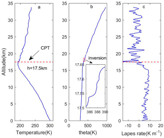
Figure 1.
(a) The temperature profile (the red dotted line indicates the cold point tropopause (CPT), and the height is 17.5 km). (b) The potential temperature profile, where the profile in the red box is enlarged to observe the inversion areas. (c) Temperature lapse rate at 12 UT on 31 May 2018.
In order to calculate the noise in the data, the entire profile is divided into several segments with an interval of 50 m; the data in each segment are linearly fitted and smoothed to obtain a data trend, and the residual is obtained by calculating the difference between the original data and the fitted data. The variance of the first difference of the residual from each piece of data is an estimate of twice the noise variance, and then the noise standard deviation can be calculated as the square root of the noise variance (it should be noted that an unavoidable problem is that this estimated noise inherently includes not only pure noise but also some small-scale perturbations). The profile is derived from the pressure and temperature data, so the standard deviation of , written as , must be calculated from the temperature noise standard deviation and the pressure noise standard deviation through the error transfer formula [29]:
Figure 2 shows the noise estimation levels for temperature, pressure and potential temperature. The average of is 0.0448 K. The basic variation in temperature noise is small, except for the large deviation near the tropopause. The average value of is 0.0492 hPa. The noise from the pressure sensor decreases rapidly with the increase in altitude. The noise of potential temperature essentially depends on the noise of temperature measurements. However, since the temperature noise does not show a clear increasing trend above 20 km, the increase in potential temperature noise is inseparable from the rapid decrease in air pressure, which also shows that the application of the Thorpe method is limited by altitude [8].
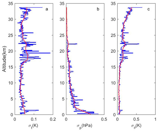
Figure 2.
Noise standard deviation of (a) temperature, (b) pressure and (c) potential temperature (red curve: smoothed profiles of these noise estimates).
In order to reflect the degree of noise interference of the sensors, the concept of the bulk trend-to-noise ratio (tnr) is introduced here to reflect the stratification stability of the atmosphere [37]:
where n is the sample size of the interval (here, we take the interval as 200 m, and n is 40), and is the average of in the interval. The values in the troposphere and stratosphere are calculated separately. When is less than 1, the atmosphere has weak stratification stability, and artificial inversion easily occurs. The Thorpe analysis is seriously affected by noise and cannot determine the upper and lower boundaries of the inversion, and filtering and undersampling of data are required at this time. The undersampling factor is selected as m (in different data sets, m may vary: generally, it is 2 or 3 in the troposphere and 1 or 2 in the stratosphere), which can satisfy the tnr of undersampled data greater than 1.5 [27]. Furthermore, the concept of the Ozmidov scale is relevant for stratified turbulence only, so in the weak stratification region at night, filtering and undersampling are needed before the turbulence parameters are calculated.
R. Wilson et al. proposed a method based on optimized filtering and statistical testing to select the real overturn by comparing the range of a data sample with the range of a normally distributed population of the same size as the data sample [37]. The basic principle is as follows: if the sample size within an inversion is n (n > 2), then the range of within the inversion is , where . The sample range caused by pure noise from Monte Carlo simulation is , showing percentiles of the range of n independent identically distributed (iid) variables (here, we set the subscript as 95, corresponding to the significance level ), and the noise standard deviation of is calculated as . If , then the inversion can be selected as the real overturn. Otherwise, the inversion is rejected as artificial noise.
3. Results and Discussion
3.1. Case Analysis
The source of energy for turbulence is mainly mechanical movement work and buoyancy work. According to this energy theory, there are mainly three ways to generate turbulence. One is the turbulence caused by wind shear and topographic factors near the ground, and the energy is generated by tangential stress. The second is the turbulence that occurs in the region with thermal instability; its energy is produced by work done by buoyancy. The third is the turbulence caused by waves and wind shear that is large enough to flip the density of the upper and lower layers, and the gravity wave breaks because the amplitude is increasing. The waves generated at this density interface are called Kelvin–Helmholtz waves. Clear air turbulence is usually thought to be caused by the breaking up of the Kelvin–Helmholtz wave [38]. What needs to be explained here is that the concept of the Ozmidov scale is relevant for stratified turbulence only. It has no meaning for convective-driven turbulence. Therefore, in the following, we do not discuss the results of the boundary layer.
Since the balloon does not rise at a constant speed, the vertical resolution of the data is uneven, and the original data are reinterpolated according to the average step size (5 m). When calculating the Richardson number here, the average value of five consecutive points is used to obtain the wind speed and the potential temperature at an interval of 25 m. The gradient Richardson number can be characterized by
where corresponds to () when the air is unsaturated (saturated). is calculated over 50 m intervals. Because of the influence of small-scale fluctuations and noises, it is smoothed by five points, denoting a spatial moving average with a segment of 200 m. When < 0, the atmosphere is statically unstable, generating thermal turbulence. When 0 < < 0.25, the atmosphere is favorable for dynamic instability, and mechanical turbulence occurs. Firstly, the Thorpe method is applied to a finite number of radiosonde data to verify the feasibility of turbulence retrieval. We use wind shear, buoyancy frequency and the Richardson number to describe atmospheric instability.
Figure 3a–h respectively show the profiles of potential temperature, vertical wind shear (the square root of the denominator of the fraction in Equation (14), buoyancy frequency, gradient Richardson number, horizontal wind component, Thorpe length, energy dissipation rate and turbulent diffusivity calculated at 12 UT on 31 May 2018. In Figure 3b, the maximum wind shear is between 18 and 20 km and is significantly higher than the surrounding area, which is caused by the tropical easterly jet stream. The buoyancy frequency in Figure 3c is significantly larger in the stratosphere than that in the troposphere. There are some negative values of buoyancy frequency in the troposphere, corresponding to the static instability region in the atmosphere, while in the stratosphere, buoyancy frequency is mainly dominated by positive values. Figure 3d shows that there are significant differences in the main mechanisms of turbulence between the stratosphere and the troposphere. Regions where < 0 and 0 << 0.25 both exist in the troposphere, indicating that there is both thermal and mechanical turbulence in the troposphere. In the stratosphere, the Richardson number is significantly increased, showing that there is mainly mechanical turbulence in the stratosphere. Figure 3e shows that the meridional and zonal components of the smoothed horizontal wind speed vary with height. It can be seen that the zonal wind is significantly larger than the meridional wind, and the values of u and v are significantly increased near the tropopause where the upper-level jet stream is formed. Figure 3f shows the distribution of the Thorpe length after the real overturn is selected. The maximum value of is around 10 km, corresponding to the area with the largest wind shear. The distribution of is mainly concentrated between 10 and 20 km. The turbulence with static instability in the troposphere is widespread, corresponding to the relatively large Thorpe scale, while static instability in the stratosphere is rare, and the inversion scale of the profile is small, with a correspondingly small Thorpe’s scale. Figure 3g,h represent the distribution of the energy dissipation rate and the turbulent diffusion coefficient with height, respectively. It can be seen that the trends of the two have a good consistency. According to the formula of the turbulent diffusion coefficient calculated by the Thorpe method, , it can be seen that their small differences in the changing trend are due to the buoyancy frequency. The region where the maximum value of and exist match the region of the maximum value of the Thorpe length. It should be noted here that the instantaneous profile of is calculated according to whether the water vapor is saturated, and and are respectively selected to eliminate small-scale fluctuations and noise; a moving average in 200-m steps is applied to to obtain . When calculating and , we use the positive buoyancy frequency calculated from the sorted potential temperature profile.
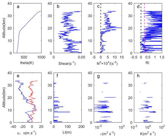
Figure 3.
At 0012 UT on 31 May 2018, (a) temperature, (b) vertical shear of wind speed, (c) buoyancy frequency, (d) gradient Richardson number, (e) wind speed component (latitude component: blue solid curve; meridional component: red solid curve), (f) Thorpe length, (g) energy dissipation rate, (h) turbulent diffusivity profile.
To make the results more universally applicable, the cumulative profile distribution from May 10 to 31 May 2018 is shown in Figure 4. The wind shear decreases with height and then increases. The maximum value of wind shear is present near the tropopause, corresponding to the upper-level jet stream near the tropopause. The negative value of buoyancy frequency is more common in the upper troposphere, indicating that the static stability of the atmosphere decreases first and then increases with height. The above results show that static instability and dynamic instability coexist over the entire troposphere height range, while in the stratosphere, the atmosphere is dominated by dynamic instability. Thorpe’s length is obviously greater in the troposphere than that in the stratosphere.
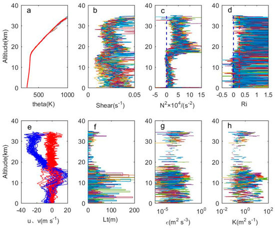
Figure 4.
At 0012 UT on 10–31 May 2018 (a) temperature, (b) vertical wind shear, (c) buoyancy frequency, (d) gradient Richardson number, (e) wind speed component (zonal component: solid blue curve; meridional component: solid red curve), (f) Thorpe length, (g) energy dissipation rate, (h) diffusion coefficient.
It should be noted that we dropped the daytime data to avoid the interference of instrument noise and weak stratification, which are not suitable for Thorpe analysis [39,40]. Especially in the middle and upper troposphere in the daytime, the noise cannot be completely eliminated, which can cause a mixture of noise and turbulence, resulting in a thicker turbulent patch, so the retrieval result at night is closer to the real state of the atmosphere. Above 30 km, and become markedly concentrated and strengthened; this is the result of the abnormally increased Lt. We believe that because the tnr is relatively small above 30 km, small-scale turbulence is easily confused with increasing noise, resulting in a significantly larger Thorpe length. Therefore, in later discussions, our analysis of turbulence parameters is limited to 30 km.
To explore the statistical results and temporal evolution of turbulence parameters, we applied the Thorpe method to balloon sounding data in the Guam area in 2013–2018. A total of 2086 profiles were collected for these six years (for some days, the measurements are missing, and for other days, they are not adopted because the maximum height that the released balloon can detect is too low). It should be noted that the turbulence scale has anisotropy in the three-dimensional space. Here, we discuss the distribution rule of the turbulent vertical scale according to the calculation results of the sounding data.
3.2. Background Wind Field, Local Instability and Occurrence Rates of Turbulence
We calculated the wind component, wind shear and buoyancy frequency for a total of six years to reflect the atmospheric instability. The data are monthly averaged values, and the parameters at the vertical height are averaged at intervals of 200 m. Figure 5 shows the monthly averaged zonal wind, meridional wind, shear and squared Brunt–Väisälä frequency from 2013 to 2018. Figure 5a shows the zonal wind speeds, and Figure 5b shows the meridional wind speeds. Zonal wind speeds range from −40 to 20 m/s, meridional wind speeds range from −10 to 10 m/s, and they all show significant annual oscillations (AO). From Figure 5c, we can see that there is a large wind shear near the ground, and the wind shear decreases gradually as the height increases. There is a small wind shear between 11 and 15 km, indicating relatively weak stratification stability. The existence of jet streams near the tropopause and in the stratosphere allows the wind shear to return to a higher level. Figure 5d shows the static stability of the atmosphere through the squared Brunt–Väisälä frequency. The stratospheric atmosphere has a strong stratification, while the middle and upper troposphere has a weak stratification, with a small buoyancy frequency between 11 and 15 km. Under the above atmospheric conditions, turbulence can be generated in various ways, including the fragmentation of gravity waves caused by wind shear, the wind shear near the jet stream, the work done by convection instability [41], the larger wind shear near the ground and gravity waves excited by terrain [42,43,44,45]. Long-term wind field variation indirectly promotes turbulence by affecting gravity wave activity and shear instability.
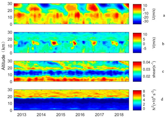
Figure 5.
The monthly averaged (a) zonal wind, (b) meridional wind, (c) shear, (d) squared Brunt–Väisälä frequency from 2013–2018.
Because turbulence is highly intermittent and random in space and time, it is more reasonable to express the frequency of turbulence in terms of the occurrence rates in a fixed area. Figure 6a shows the monthly means for the Thorpe length , Figure 6b shows the monthly occurrence rates of , Figure 6c shows the monthly occurrence rates of and Figure 6d shows the monthly occurrence rates of . The maximum value of is distributed between 12 and 16 km below the cold point tropopause, which can reach over 100 m, and the value has pronounced seasonal variation. The maximum of within this height range usually occurs from July to September. We call it the “strongest turbulent mixing band,” corresponding to the region where the monthly occurrence rates of and the monthly occurrence rates of are both higher. The occurrence rates of turbulence in this region can also reach more than 60%, indicating that turbulent mixing easily occurs in this region as a result of weak laminar stability, including mechanical turbulence and thermal turbulence. The monthly occurrence rates of turbulence below 10 km are probably around 20%, and the corresponding monthly means for the Thorpe length are within 50 m. The turbulence in this region is caused by both convective instability () and dynamic instability (), and the turbulence near the ground is mainly generated by the dynamic instability caused by topography and wind shear. In the stratosphere, however, the occurrence rate of turbulence is much lower, corresponding to a smaller turbulence scale and intensity, and turbulence in this region is mostly caused by dynamic instability. In the stratosphere, the variation law for the occurrence rates of is highly consistent with the strongest turbulent mixing band; it can be reduced from 10% in July–September to less than 1% in the other months. According to Figure 6, it can be observed that turbulent mixing in the weak stratification region has a high intensity and a larger Thorpe length, corresponding to larger turbulence intensity, while in the static stable region, the exchange of materials and energy between the upper and lower layers is weak, and the Thorpe length is smaller, corresponding to lower turbulence intensity.
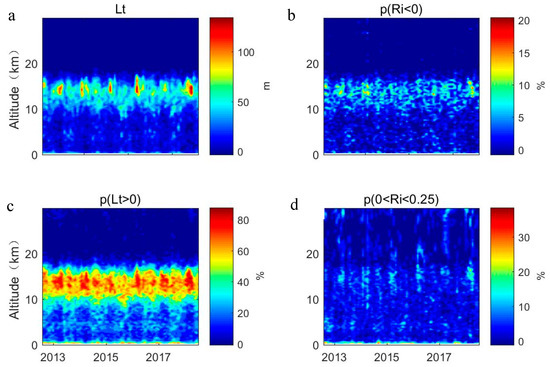
Figure 6.
(a) Monthly means for the Thorpe length , (b) monthly occurrence rates of , (c) monthly occurrence rates of , (d) monthly occurrence rates of .
3.3. Distribution of Turbulent Overturn Size, Energy Dissipation Rate and Diffusion Coefficient
The turbulent overturn size can be represented as the vertical thickness of an independent turbulent patch, and the thickness is calculated as , where a and b denote the lowermost and uppermost bin of the patch, and is the average sampling step. The turbulent energy dissipation rate and turbulent diffusion coefficient determine the ability of the flow to maintain turbulence or develop into turbulence. and need to be calculated precisely, as they can control the transport of matter and energy in the atmosphere.
3.3.1. Distribution Characteristics of the Statistical Histogram
Figure 7a–b shows the frequency distribution of the turbulence overturn size from 2013 to 2018 in the troposphere and stratosphere, respectively. Generally speaking, the amount of turbulence decreases with the increase in the overturn size, and the scale of turbulence is dominated by a small scale. However, limited by the resolution of the sensor, the minimum overturn size detected here is 10 m. Through the experimental results of [25], we know that the turbulence detected by low-resolution detection (5–9 m) in the troposphere is only 7% of the high-resolution detection (10–20 cm), while in the stratosphere, the value is reduced to 4%. That is to say, the smaller-scale turbulence is undetectable, so the exploration of turbulence characteristics in this paper is based on the turbulence of a large vertical scale. In the troposphere, the most abundant turbulence scale is between 100 and 200 m, accounting for 34.2% of the total turbulence, while in the stratosphere, the most abundant turbulence scale is below 100 m, accounting for 73.0% of the total turbulence. The overturn size that exceeds 100 m accounts for 75.5% in the troposphere, and even 39.7% of the turbulence scales can exceed 500 m. As for the stratosphere, the overturn size that exceeds 500 m only accounts for 3.0% of the total turbulence.
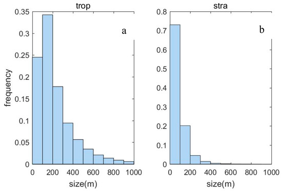
Figure 7.
Turbulence overturn size from 2013 to 2018. (a) The frequency distribution in the troposphere, (b) the frequency distribution in the stratosphere.
The number of turbulence layers in the troposphere (stratosphere) accounts for 82% (18%) of the total. The amount of turbulence detected in the troposphere is far more than that in the stratosphere. In the stratosphere, the stratification is stable, the buoyancy work is relatively difficult, and the convective exchange of the upper and lower layers is weak. Therefore, the Thorpe displacement of a single particle is small, and the thickness of the independent overturn region calculated by the Thorpe method is relatively thin, which leads to the relatively small thickness of the turbulent patch. Strong wind shear in the stable stratified atmosphere will cause the atmospheric density to invert up and down, causing the amplitude of the gravity wave to increase and then break, resulting in clear-air turbulence (CAT), which is also the main form of turbulence in the stratosphere.
Figure 8a,b shows the frequency distribution of in the troposphere and stratosphere. Figure 8c,d show the same distribution but for . The magnitude of is between 10-6 and 100 m2 s−3, which is mainly distributed between 10−4 and 10−2 m2 s−3 in the troposphere, accounting for 71.48% of the total and between 10−5 and 10−3 m2 s−3 in the stratosphere, accounting for 76.67% of the total. The magnitude of is between 10−2 and 102 m2 s−1, which is mainly distributed between 10−1 and 101 m2 s−1 in the troposphere, accounting for 78.64% of the total and between 10−2 and 100 m2 s−1 in the stratosphere, accounting for 90.82% of the total. Regardless of whether it is in the stratosphere or troposphere, has a normal distribution; the mean value in the troposphere is 0.0068, as computed by , and the standard deviation is 1.0060, as computed by . In the stratosphere, the mean value is 0.0016, and the standard deviation is 0.8171. has an apparent normal distribution only in the troposphere. Regardless of whether we examine or , the main frequency distribution area in the troposphere is an order of magnitude higher than that in the stratosphere. If the turbulence is divided into strong turbulence according to the value of the energy dissipation rate ( > 10−4 m2 s−3) and weak turbulence ( < 10−4 m2 s−3) [46], strong turbulence accounts for 77.48% in the troposphere and 65.98% in the stratosphere. The proportion of strong turbulence over the entire detection height is 74.27%.
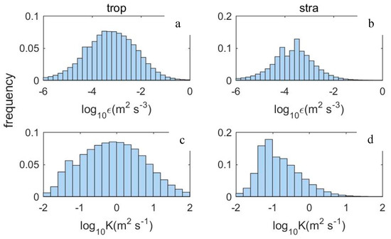
Figure 8.
Histogram of the frequency distribution of (a) tropospheric energy dissipation rate, (b) stratospheric energy dissipation rate, (c) tropospheric diffusion coefficient, (d) stratospheric diffusion coefficient.
3.3.2. Distribution Characteristics of Time Series
In order to explore the characteristics of the temporal and spatial distribution of the turbulence thickness, turbulent energy dissipation rate and diffusion coefficient, the height is stratified at intervals of 200 m, and the monthly average is taken. According to the previous statistical distribution results, turbulence patches with thicknesses of more than 1000 m are discarded, and the ranges of and are set at 10−6–100 m2 s−3 and 10−2–102 m2 s−1, respectively.
Figure 9 shows the time series of atmospheric column characteristics from 2013 to 2018; Figure 9a–c show the monthly means of the turbulence thickness, turbulent energy dissipation rate and turbulent diffusion coefficient, respectively. There is a region with large turbulence scales that range between 11 and 16 km, in which the maximum turbulence thickness also appears in July–September every year, showing the same annual oscillations (AO) as the Thorpe length since they are directly physically related. Turbulence scales in this region range from 300 to 1000 m. Below 10 km, the turbulence thickness is within 200 m, and the thickness also varies alternately with time. In the stratosphere, the turbulence thickness is relatively small, with the average scale not exceeding 10 m after a 200 m vertically spaced average. The energy dissipation rate and turbulent diffusivity have the same distribution characteristics as the overturn size in the troposphere. From July to September, compared with other months, there are larger values of and in the upper troposphere, while the smaller values of and remain in the lower troposphere.
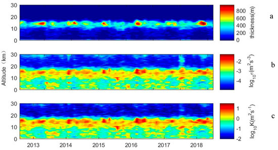
Figure 9.
Time series of atmospheric column characteristics from 2013 to 2018: (a) overturn size, (b) turbulent kinetic energy dissipation rate, (c) turbulent diffusion coefficient.
It can be seen from Equations (5) and (6) that the values of and are affected by the value of , and the extreme value distribution area of is also the extreme value distribution area of and . Although is related to , it is also related to the buoyancy frequency according to the Thorpe method. Specifically, the variables in Equation (5) include and . is significantly increased, while is significantly decreased in the stratosphere, and the term has a more obvious impact than the term. Therefore, in the stratosphere, can still be larger, though the value of is relatively small. This also shows that under the condition of stable stratification, even if turbulent overturn does not easily occur or if the turbulence scale is small, a relatively large energy dissipation rate can still exist. In other words, small-scale turbulence in a stratified stable atmosphere can also generate fast energy dissipation. The subterms in Equation (6) include and ; the magnitude of is much larger than that of , and is a quadratic term, while is in the first degree, so the value of is more susceptible to the term. The values of and have almost consistent variation trends in the troposphere, but for the stratosphere, although there is an interval with a relatively large value of , it corresponds to a relatively small value of , which indicates that it is in the unstable region of the atmosphere. The larger turbulent scale corresponds to stronger dissipation and diffusion, while in the stable region of the atmosphere, where the turbulence scale is usually small, the turbulent diffusion is weak, while the energy dissipation is strong.
3.3.3. Profile Distribution Characteristics of Multiyear Monthly Averages
The results in the previous discussion clearly demonstrate the annual oscillation characteristics of turbulence parameters, and the period from July to September is when the turbulence scale and turbulence intensity are significantly enhanced. Therefore, we divided the six-year data into four groups: January–March, April–June, July–September and October–December; the data in each group were averaged according to a height interval of 2 km to obtain the distribution characteristics of the turbulence parameters with height in different seasons. The result is shown in Figure 10. Figure 10a–d shows the vertical distribution of , , turbulence thickness and Thorpe length, respectively (blue: January–March; red: April–June; magenta: July–September; cyan: October–December). The averaging was done across the whole data set.
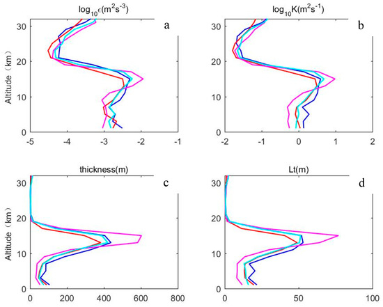
Figure 10.
Seasonal vertical profiles of the median values of (a) the logarithm of , (b) the logarithm of , (c) turbulent thickness, (d) Thorpe length (blue: January–March; red: April–June; magenta: July–September; cyan: October–December).
It can be seen from the results that the distribution characteristics of the turbulence scale, turbulence intensity, turbulent energy dissipation rate and turbulent diffusion coefficient have significant seasonal differences with height. The turbulent energy dissipation rate and turbulent diffusion coefficient change little with heights below 7 km; the values of are distributed between 0.0010 and 0.0032 m2 s−3, and the values of are distributed between 0.5 and 1.9 m2 s−1. They both reach the maximum value at around 15–16 km, and their values from July to September are significantly higher than those in the other months. The maximum values of and can reach 0.0116 m2 s−3 and 9.7 m2 s−1, respectively, from July to September. From 15 to 23 km, and decrease significantly and reach their minimum value at 23 km, which is 3 × 10⁻⁵ m2 s−3 and 0.0163 m2 s−1, respectively. Above 23 km, they both increase with altitude.
The turbulence scale and Thorpe length are consistent with the variation trend of and below 20 km. Below 7 km, the average turbulence thickness is within 100 m, and the average Thorpe length is between 8 and 20 m. Between 7 and 20 km, the turbulence scale and Thorpe length increase rapidly with height and reach the maximum value at around 15 km, which is 600 and 77 m, respectively, and then they decrease rapidly with height. Above 20 km, the mean values of turbulence thickness and length are close to 0, indicating only sporadic small turbulence above this height.
It can be seen that significantly enhanced turbulence parameters are concentrated between 14 and 16 km for all balloon flights. The obvious enhancement of turbulent mixing near the tropopause is a long-term stable feature over Guam. Figure 11 shows the average profile distribution of the atmospheric background field. Wind shear, horizontal wind field and buoyancy frequency are averaged at an altitude interval of 1 km. This turbulent layer may be mainly caused by static instability as at this level reaches the minimum value. Another possible cause is the intense shear instability in trop-stratospheric jet streams. There is more intense turbulence activity in the height range from July to September compared with the annual average level. This is because there is a stronger horizontal wind field near the tropopause from July to September, where meridional and zonal winds increase significantly, which can lead to significantly increased wind shear. At the same time, between 15 and 19 km, the rapid increase in with height will lead to an increase in the amplitude of the gravity wave [47], and the strong wind shear within the corresponding height will lead to the breakup of the gravity wave and produce turbulence.
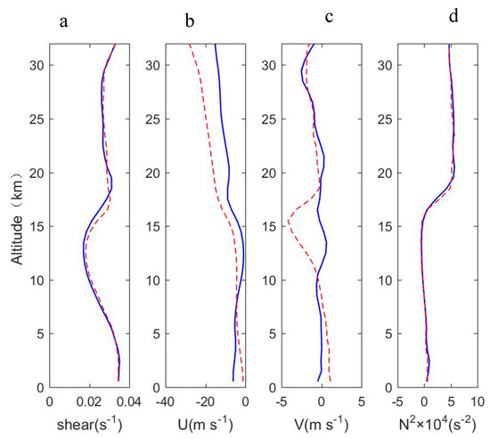
Figure 11.
Vertical profiles of (a) wind shear, (b) zonal wind, (c) meridional wind, (d) buoyancy frequency (solid blue line: monthly means from 2013 to 2018; red dotted line: the means over six years, from July to September).
3.4. Overview and Discussion
The results show that p( > 0) exceeds 60% in the altitude range of 12–16 km, and it decreases to a level below 10% above 20 km. In Zhang’s research [27], p( > 0) varies from as high as 90% in the altitude range of 9–11 km to around 10% above 25 km. He et al. [8] also show that the area with the strongest turbulent activity is around 10 km. Zhou [48] proposed the concept of the “Strongest Mixed Layer,” that is, the area of the maximum value of . The result shows that the height of the strongest mixing layer gradually decreases from the equator to the poles, which is a direct consequence of the fact that the height of the tropopause increases from the poles to the equator. Considering the different areas studied, this is also the reason that the extreme regions of Thorpe length are not the same in different studies. The overturn size, turbulent kinetic energy dissipation rate and turbulent diffusion coefficient also show obvious annual oscillations (AO), consistent with . It is worth noting that low-value areas with buoyant frequencies near the tropopause also correspond to areas where the Richardson number is weak, indicating that turbulence is more likely to occur near the upper troposphere than the lower troposphere. As can be seen from the results, the turbulent maximum mixing zone corresponds to the minimum value of static stability, the maximum value of wind speed and the minimum value of vertical shear. Considering that the gravity wave activity will reduce the local static stability [49], the small average wind shear is sufficient to induce Kelvin–Helmholtz instability. This phenomenon is also consistent with the result of [50], which shows that the low-frequency gravity wave easily induces Kelvin–Helmholtz instability. In other words, the gravity wave activity can reduce the static stability, so small vertical shear is also prone to dynamic instability [51]. The vertical scale of turbulence is considerably larger than that in other regions; this is referred to as the “strongest turbulent mixing band” in this article. Its existence is very important for the material exchange and interaction between the troposphere and stratosphere [52].
At a given time, if the turbulence scale in the upper troposphere is relatively large, then the turbulence scale in the lower troposphere is relatively small and vice versa. The same occurs with ε, K and even wind speed. Because the tropical western Pacific is the main area where Madden–Julian Oscillation (MJO) occurs, it has an approximate barometric vertical structure, showing that the zonal wind field tilts westward with height. The antiphase of the upper and lower troposphere appears. We speculate that this may be a possible reason that the turbulent activity at the corresponding height presents a similar antiphase; however, this needs to be further demonstrated. Because of the seasonal evolution of the Earth’s orbital parameters, the direct solar point moves from north to south with the seasons, and the influence of the sun on the region also changes throughout the year. Considering that the direct solar point is passing through the tropical western Pacific from north to south at this time, a significant increase in turbulence activity may occur from July to September. Kohma et al. [26] mentioned that seasonal variation in radar-based ε shows a broad maximum in August–October and low values in November–January in the lower stratosphere, which is similar to our results. The statistical characteristics of gravity waves at Gadank, which has the same latitude as Guam, are discussed in detail in [53,54,55], which have a certain reference significance for the turbulence distribution characteristics in this paper. Clear seasonal variation in the wave activity was noted in their study, and during the monsoon season, they found that the significant enhancement of gravity wave activity was related to the westward phase of the zonal wind. In the results in this paper, the turbulence enhancement area in the strongest mixing zone also corresponds to the westward propagation of the zonal wind, indicating a correlation between turbulence and the gravity wave activity behind it.
All our results show that regardless of the variation in time and space, there is always a strong turbulent mixing band with significant AO caused by both shear instability and static instability near the tropopause, and it is localized in the portion of the wave characterized by reduced static stability where the turbulence activity is markedly enhanced. These results can be used for reference to understand the turbulence characteristics over the tropical Western Pacific Ocean [56,57,58,59], and the continuous high-resolution radiosonde data can also be helpful for model calibration and the verification of turbulence parameters. The link between the gravity wave and turbulence is worthy of further study, and the roles that they play in the complex air–sea system of the tropical western Pacific need further research.
4. Conclusions
This paper analyzes high-resolution radiosonde data over the Guam area from 2013 to 2018 by the Thorpe method. Time series characteristics and multiyear statistical distribution characteristics of atmospheric turbulence parameters are explored, and the main conclusions are as follows.
The analysis of instrument noise from the measured data shows that the instrument noise level increases with height, and after reaching a certain height, the potential temperature noise increases rapidly with the rapid decrease in air pressure, which can lead to confusion between the small turbulence layer and the high noise in the stratosphere (above 30 km), resulting in an anomalous larger turbulence layer. According to the results in this paper, the Guam radiosonde can be adapted to the Thorpe method at altitudes below 30 km. In general, the Thorpe method applies well to the data of the US high-resolution balloon sensor in the Western Pacific Ocean. The value of is mainly distributed between 10−4 and 10−2 m2 s−3 in the troposphere and 10−5 and 10−3 m2 s−3 in the stratosphere, exhibiting normal distribution characteristics. The value of is mainly distributed between 10−1 and 101 m2 s−1 in the troposphere and 10−2 and 100 m2 s−1 in the stratosphere.
The distributions of the Richardson number, buoyancy frequency and wind shear are used to explore the atmospheric unstable state. There is mainly sporadic mechanical turbulence in the stratosphere, while thermal turbulence and mechanical turbulence are both involved in the troposphere. The intensity and quantity of turbulence in the troposphere are greater than those in the stratosphere. In the instability region, the greater turbulence overturn leads to a stronger turbulent kinetic energy (TKE) dissipation rate and turbulent diffusivity; in the stable region, the turbulent overturn is small, and the turbulent diffusion is weak, but there is strong energy dissipation. The thermal turbulence is dominated by large eddies, and the mechanical turbulence is dominated by small eddies. The turbulence detected in the troposphere is mainly over 100 m, and the turbulence detected in the stratosphere is mainly below 100 m. Limited by the resolution of sensors, the minimum scale of turbulence that can be observed is 10 m, which means that high-resolution balloon sensors can only detect a few large-scale turbulences.
Turbulence is most likely to occur between 10 and 16 km, where thermal instability and shear instability both exist. There is a perennial, stable turbulent mixing band below the cold point tropopause, where the turbulence scale, turbulence intensity, turbulent energy dissipation rate and turbulent diffusion coefficient are significantly enhanced. The strong turbulent mixing band is mainly dominated by large eddies and has pronounced annual oscillation characteristics. The time period during which the turbulence parameter is significantly enhanced is from July to September, corresponding to the passing of the direct solar point over the station from north to south and significantly enhanced wind speed over this height range. This work has the potential to aid in the improvement of free atmosphere turbulence representations in global models.
Author Contributions
Y.H. and Z.S. designed the experiments; Y.H., Z.S., M.H., L.Z. and S.Z. performed the experiments; M.H., Z.S., L.Z. and S.Z. analyzed the data; Y.H. wrote the paper. All authors have read and agreed to the published version of the manuscript.
Funding
This work was supported by the National Natural Science Foundation of China (Grant no. 41875045, 41576171, 41775039).
Conflicts of Interest
The authors declare no conflict of interest.
References
- Riveros, H.G.; Riveros-Rosas, D. Laminar and turbulent flow in water. Phys. Educ. 2010, 45, 288–291. [Google Scholar] [CrossRef]
- Belu, R.; Jumper, G. Gravity Waves and Turbulence as Seen in the Radiosonde-Thermosonde Observations. In Proceedings of the 7th AIAA Aerospace Sciences Meeting including the New Horizons Forum and Aerospace Exposition, Orlando, FL, USA, 5–8 January 2009. [Google Scholar]
- Zhao, X.R.; Sheng, Z.; Li, J.W.; Yu, H.; Wei, K.J. Determination of the “wave turbopause” using a numerical differentiation method. J. Geophys. Res. Atmos. 2019, 124, 10592–10607. [Google Scholar] [CrossRef]
- Wang, W.; Shangguan, M.; Tian, W.; Schmidt, T.; Ding, A. Large uncertainties in estimation of tropical tropopause temperature variabilities due to model vertical resolution. Geophys. Res. Lett. 2019, 46, 10043–10052. [Google Scholar] [CrossRef]
- Zhang, J.; Tian, W.; Chipperfield, M.P.; Xie, F.; Huang, J. Persistent shift of the Arctic polar vortex towards the Eurasian continent in recent decades. Nat. Clim. Chang. 2016, 6, 1094–1099. [Google Scholar] [CrossRef]
- Zhang, J.; Tian, W.; Xie, F.; Chipperfield, M.P.; Feng, W.; Son, S.W.; Abraham, N.L.; Archibald, A.T.; Bekki, S.; Butchart, N.; et al. Stratospheric ozone loss over the Eurasian continent induced by the polar vortex shift. Nat. Commun. 2018, 9, 1–8. [Google Scholar] [CrossRef]
- Zaichik, L.I.; Alipchenkov, V.M. A statistical model for transport and deposition of high-inertia colliding particles in turbulent flow. Int. J. Heat Fluid Flow 2001, 22, 365–371. [Google Scholar] [CrossRef]
- He, Y.; Sheng, Z.; He, M. The First Observation of Turbulence in Northwestern China by a Near-Space High-Resolution Balloon Sensor. Sensors 2020, 20, 677. [Google Scholar] [CrossRef]
- Hu, D.; Guan, Z.; Tian, W.; Ren, R. Recent strengthening of the stratospheric Arctic vortex response to warming in the central North Pacific. Nat. Commun. 2018, 9, 1697. [Google Scholar] [CrossRef]
- Hu, D.; Tian, W.; Xie, F.; Wang, C.; Zhang, J. Impacts of stratospheric ozone depletion and recovery on wave propagation in the boreal winter stratosphere. J. Geophys. Res. Atmos. 2015, 120, 8299–8317. [Google Scholar] [CrossRef]
- Xie, F.; Li, J.; Zhang, J.; Tian, W.; Hu, Y.; Zhao, S.; Sun, C.; Ding, R.; Feng, J.; Yang, Y. Variations in north Pacific sea surface temperature caused by Arctic stratospheric ozone anomalies. Environ. Res. Lett. 2017, 12, 114023. [Google Scholar] [CrossRef]
- Saad, T. Turbulence Modeling for Beginners; University of Tennessee Space Institut: Tullahoma, TN, USA, 2011. [Google Scholar]
- Thorpe, S.A. Turbulence and Mixing in a Scottish Loch. Philosophical Transactions of the Royal Society A: Mathematical. Phys. Eng. Sci. 1977, 286, 125–181. [Google Scholar] [CrossRef]
- Haack, A.; Gerding, M.; Lübken, F.J. Characteristics of stratospheric turbulent layers measured by LITOS and their relation to the Richardson number. J. Geophys. Res. 2014, 119, 10605–10618. [Google Scholar] [CrossRef]
- Gavrilov, N.M.; Luce, H.; Crochet, M.; Dalaudier, F.; Fukao, S. Turbulence parameter estimations from high-resolution balloon temperature measurements of the MUTSI-2000 campaign. Ann. Geophys. 2005, 23, 2401–2413. [Google Scholar] [CrossRef]
- Johnson, H.L.; Garrett, C. Effects of Noise on Thorpe Scales and Run Lengths. J. Phys. Oceanogr. 2004, 34, 2359–2372. [Google Scholar] [CrossRef]
- Thorpe, S.A. The Turbulent Ocean; Cambridge University Press: Cambridge, UK, 2005; 439 p. [Google Scholar] [CrossRef]
- Lorke, A.; Wüest, A. Probability density of displacement and overturning length scales under diverse stratification. J. Geophys. Res. Oceans 2002, 107, 7–11. [Google Scholar] [CrossRef][Green Version]
- Dillon, T.M. Vertical overturns: A comparison of Thorpe and Ozmidov length scales. J. Geophys. Res. 1982, 87, 9601. [Google Scholar] [CrossRef]
- Li, D.; Salesky, S.T.; Banerjee, T. Connections between the Ozmidov scale and mean velocity profile in stably stratified atmospheric surface layers. J. Fluid Mech. 2016, 797. [Google Scholar] [CrossRef]
- Clayson, C.A.; Kantha, L. On turbulence and mixing in the free atmosphere inferred from high-resolution soundings. J. Atmos. Ocean. Technol. 2008, 25, 833–852. [Google Scholar] [CrossRef]
- Wesson, J.C.; Gregg, M.C. Mixing at Carmirana Sill in the Strait of Gibraltar. J. Geophys. Res. 1994, 99, 9847–9878. [Google Scholar] [CrossRef]
- Fer, I. Mixing of the Storfjorden overflow (Svalbard Archipelago) inferred from density overturns. J. Geophys. Res. 2004, 109, C01005. [Google Scholar] [CrossRef]
- Nath, D.; Ratnam, M.V.; Patra, A.K.; Murthy, B.V.K.; Rao, S.V.B. Turbulence characteristics over tropical station Gadanki ( 13.5° N,79.2° E)estimated using high-resolution GPS radiosonde data. J. Geophys. Res. 2010, 115, 1–13. [Google Scholar] [CrossRef]
- Wilson, R.; Dalaudier, F.; Luce, H. Can one detect small-scale turbulence from standard meteorological radiosondes? Atmos. Meas. Tech. 2011, 4, 795–804. [Google Scholar] [CrossRef]
- Kohma, M.; Sato, K.; Tomikawa, Y.; Nishimura, K.; Sato, T. Estimate of Turbulent Energy Dissipation Rate from the VHF Radar and Radiosonde Observations in the Antarctic. J. Geophys. Res. Atmos. 2019, 124, 2976–2993. [Google Scholar] [CrossRef]
- Zhang, J.; Zhang, S.D.; Huang, C.M.; Huang, K.M.; Gong, Y.; Gan, Q.; Zhang, Y.H. Statistical Study of Atmospheric Turbulence by Thorpe Analysis. J. Geophys. Res. Atmos. 2019, 124, 2897–2908. [Google Scholar] [CrossRef]
- Kvasov, B.I. Cubic Spline Interpolation. In Methods of Shape-Preserving Spline Approximation; World Scientific Pub Co Inc, SG: Singapore, 2000. [Google Scholar] [CrossRef]
- Wilson, R.; Luce, H.; Hashiguchi, H.; Shiotani, M.; Dalaudier, F. On the effect of moisture on the detection of tropospheric turbulence from in situ measurements. Atmos. Meas. Tech. Discuss. 2013, 5, 697–702. [Google Scholar] [CrossRef]
- Zhang, J.; Chen, H.; Li, Z.; Fan, X.; Peng, L.; Yu, Y.; Cribb, M. Analysis of cloud layer structure in Shouxian, China using RS92 radiosonde aided by 95 GHz cloud radar. J. Geophys. Res. Atmos. 2010, 115, 1–13. [Google Scholar] [CrossRef]
- Emanuel, K.A.; Hide, R. Atmospheric Convection. Phys. Today 2008, 48, 88–89. [Google Scholar] [CrossRef]
- Durran, D.R.; Klemp, J.B. On the Effects of Moisture on the Brunt-Väisälä Frequency. J. Atmos. Sci. 2002, 39, 2152–2158. [Google Scholar] [CrossRef]
- Cushman-Roisin, B.; Beckers, J.M. Stratification. In Introduction to Geophysical Fluid Dynamics; Academic Press: Cambridge, MA, USA, 2011. [Google Scholar] [CrossRef]
- Houry, S.; Dombrowsky, E.; De Mey, P.; Minster, J.-F. Brunt-Väisälä Frequency and Rossby Radii in the South Atlantic. J. Phys. Oceanogr. 1987, 17, 1619–1626. [Google Scholar] [CrossRef][Green Version]
- Alappattu, D.P.; Kunhikrishnan, P.K. First observations of turbulence parameters in the troposphere over the Bay of Bengal and the Arabian Sea using radiosonde. J. Geophys. Res. 2010, 115, 1–12. [Google Scholar] [CrossRef]
- Kuang, Z.; Bretherton, C.S. Convective Influence on the Heat Balance of the Tropical Tropopause Layer: A Cloud-Resolving Model Study. J. Atmos. Sci. 2004, 61, 2919–2927. [Google Scholar] [CrossRef]
- Wilson, R.; Luce, H.; Dalaudier, F.; Lefrère, J. Turbulence patch identification in potential density or temperature profiles. J. Atmos. Ocean. Technol. 2010, 27, 977–993. [Google Scholar] [CrossRef]
- Lindzen, R.S. Turbulence and stress owing to gravity wave and tidal breakdown. J. Geophys. Res. 2008, 86, 9707. [Google Scholar] [CrossRef]
- Luce, H.; Wilson, R.; Dalaudier, F.; Hashiguchi, H.; Nishi, N.; Shibagaki, Y.; Nakajo, T. Simultaneous observations of tropospheric turbulence from radiosondes using Thorpe analysis and the VHF MU radar. Radio Sci. 2014, 49, 1106–1123. [Google Scholar] [CrossRef]
- Wilson, R.; Hashiguchi, H.; Yabuki, M. Vertical spectra of temperature in the free troposphere at meso-and-small scales according to the flow regime: Observations and interpretation. Atmosphere 2018, 9, 415. [Google Scholar] [CrossRef]
- Xu, X.; Xue, M.; Wang, Y.; Huang, H. Mechanisms of secondary convection within a mei-yu frontal mesoscale convective system in Eastern China. J. Geophys. Res. Atmos. 2017, 122, 47–64. [Google Scholar] [CrossRef]
- He, Y.; Sheng, Z.; He, M. Spectral Analysis of Gravity Waves from Near Space High-Resolution Balloon Data in Northwest China. Atmosphere 2020, 11, 133. [Google Scholar] [CrossRef]
- Xu, X.; Wang, Y.; Xue, M.; Zhu, K. Impacts of horizontal propagation of orographic gravity waves on the wave drag in the stratosphere and lower mesosphere. J. Geophy. Res. 2017, 122. [Google Scholar] [CrossRef]
- Xu, X.; Song, J.; Wang, Y.; Xue, M. Quantifying the effect of horizontal propagation of three-dimensional mountain waves on the wave momentum flux using Gaussian beam approximation. J. Atmos. Sci. 2017, 74, 1783–1798. [Google Scholar] [CrossRef]
- Xu, X.; Shu, S.; Wang, Y. Another look on the structure of mountain waves: A spectral perspective. Atmos. Res. 2017, 191, 156–163. [Google Scholar] [CrossRef]
- Cho, J.Y.N.; Newell, R.E.; Anderson, B.E.; Barrick, J.W.; Thornhill, K.L. Characterizations of tropospheric turbulence and stability layers from aircraft observations. J. Geophys. Res. Atmos. 2003, 108. [Google Scholar] [CrossRef]
- Vanzandt, T.E.; Fritts, D.C. A Theory of Enhanced Saturation of the Gravity Wave Spectrum Due to Increases in Atmospheric Stability. Pure Appl. Geophys. 1989, 130, 399–420. [Google Scholar] [CrossRef]
- Sheng, Z.; Zhou, L.; He, Y. Retrieval and Analysis of the Strongest Mixed Layer in the Troposphere. Atmosphere 2020, 11, 3. [Google Scholar] [CrossRef]
- Fritts, D.C.; Dunkerton, T.J. Fluxes of heat and constituents due to convectively unstable gravity waves. J. Atmos. Sci. 1985, 42, 549–556. [Google Scholar] [CrossRef][Green Version]
- Fritts, D.C.; Rastogi, P.K. Convective and dynamical instabilities due to gravity wave motions in the lower and middle atmosphere: Theory and observations. Radio Sci. 1985, 20, 1247–1277. [Google Scholar] [CrossRef]
- Worthington, R.M. MST radar observations of turbulent altocumulus layers. Atmos. Sci. Lett. 2015, 16, 500–505. [Google Scholar] [CrossRef]
- Venkat Ratnam, M.; Narendra Babu, A.; Jagannadha Rao, V.V.M.; Vijaya Bhaskar Rao, S.; Narayana Rao, D. MST radar and radiosonde observations of inertia-gravity wave climatology over tropical stations: Source mechanisms. J. Geophys. Res. 2008, 113, D07109. [Google Scholar] [CrossRef]
- Mai, Y.; Sheng, Z.; Shi, H.; Liao, Q.; Zhang, W. Spatiotemporal Distribution of Atmospheric Ducts in Alaska and Its Relationship with the Arctic Vortex. Int. J. Antennas Propag. 2020, 13. [Google Scholar] [CrossRef]
- Leena, P.; Venkat Ratnam, M.; Krishna Murthy, B. Inertia gravity wave characteristics and associated fluxes observed using five years of radiosonde measurements over a tropical station. J. Atmos. Sol. Terr. Phys. 2012, 84–85, 37–44. [Google Scholar] [CrossRef]
- Nath, D.; Venkat Ratnam, M.; Jagannadha Rao VV, M.; Krishna Murthy, B.V.; Vijaya Bhaskara Rao, S. Gravity wave characteristics observed over a tropical station using high-resolution GPS radiosonde soundings. J. Geophys. Res. 2009, 114, D06117. [Google Scholar] [CrossRef]
- Sun, Y.; Li, T.; Zhong, Z.; Yi, L.; Chen, X.; Ha, Y.; Zhu, J.; Shen, Y.; Xu, Z.; Hu, Y. A recent reversal in the poleward shift of western North Pacific tropical cyclones. Geophys. Res. Lett. 2018, 45, 9944–9952. [Google Scholar] [CrossRef]
- Shen, Y.; Sun, Y.; Zhong, Z.; Liu, K.; Shi, J. Sensitivity Experiments on the Poleward Shift of Tropical Cyclones over the Western North Pacific under Warming Ocean Conditions. J. Meteor. Res. 2018, 32, 560–570. [Google Scholar] [CrossRef]
- Chang, S.; Sheng, Z.; Du, H.; Ge, W.; Zhang, W. A channel selection method for hyperspectral atmospheric infrared sounders based on layering. Atmos. Meas. Tech. 2020, 13, 629–644. [Google Scholar] [CrossRef]
- Shen, Y.; Sun, Y.; Camargo, S.J.; Zhong, Z. A Quantitative Method to Evaluate Tropical Cyclone Tracks in Climate Models. J. Atmos. Ocean. Technol. 2018, 35, 1807–1818. [Google Scholar] [CrossRef]
© 2020 by the authors. Licensee MDPI, Basel, Switzerland. This article is an open access article distributed under the terms and conditions of the Creative Commons Attribution (CC BY) license (http://creativecommons.org/licenses/by/4.0/).