Article

Sensitivity of a Bowing Mesoscale Convective System to Horizontal Grid Spacing in a Convection-Allowing Ensemble

by
John R. Lawson
1,2,3,*,
William A. Gallus, Jr.
3 and
Corey K. Potvin
2,4
1
Cooperative Institute for Mesoscale Meteorological Studies, University of Oklahoma, Norman, OK 73072, USA
2
NOAA/OAR/National Severe Storms Laboratory, Norman, OK 73072, USA
3
Department of Geological and Atmospheric Sciences, Iowa State University, Ames, IA 50011, USA
4
School of Meteorology, University of Oklahoma, Norman, OK 73072, USA
*
Author to whom correspondence should be addressed.
Atmosphere 2020, 11(4), 384; https://doi.org/10.3390/atmos11040384
Submission received: 24 February 2020 / Revised: 31 March 2020 / Accepted: 8 April 2020 / Published: 14 April 2020

Abstract

:
The bow echo, a mesoscale convective system (MCS) responsible for much hail and wind damage across the United States, is associated with poor skill in convection-allowing numerical model forecasts. Given the decrease in convection-allowing grid spacings within many operational forecasting systems, we investigate the effect of finer resolution on the character of bowing-MCS development in a real-data numerical simulation. Two ensembles were generated: one with a single domain of 3-km horizontal grid spacing, and another nesting a 1-km domain with two-way feedback. Ensemble members were generated from their control member with a stochastic kinetic-energy backscatter scheme, with identical initial and lateral-boundary conditions. Results suggest that resolution reduces hindcast skill of this MCS, as measured with an adaptation of the object-based Structure–Amplitude–Location method. The nested 1-km ensemble produces a faster system than in both the 3-km ensemble and observations. The nested 1-km simulation also produced stronger cold pools, which could be enhanced by the increased (fractal) cloud surface area with higher resolution, allowing more entrainment of dry air and hence increased evaporative cooling.

1. Introduction

Within the group of mesoscale convective systems (MCSs), systems that display bowing structures along the convective line are among the most poorly forecast [1]. Lawson and Gallus [2] showed that smaller (progressive) bow echoes were likely poorly forecast due to inherent low predictability more so than deficiencies in microphysical parameterizations, and that improvements in synoptic- and mesoscale initial and lateral-boundary conditions (ICs and LBCs, respectively) would yield only minor skill increases at best. The diminishing returns from more accurate large-scale ICs and LBCs were discussed by Durran and Weyn [3], and stem from the small-scale sensitivity to minuscule error on the large scale via downscale error cascade and growth [4].
Many operational centers use ensemble prediction systems (EPSs) to account for uncertainty in the forecast. Ensemble diversity is generated by, e.g., varying the ICs and LBCs, using numerous parameterizations (e.g., [5]), perturbing parameterization tendencies stochastically (e.g., [6]), and so on. Uncertainty in the forecast can be measured by the difference between the perturbation members (or spread), which represents heightened sensitivity to earlier perturbations [7]. At a given lead time, higher spread is often associated with lower skill [8], and represents lower inherent predictability and a shorter predictability time horizon [9,10]. Hence, uncertainty is an important output from an EPS in its own right. In the following sections, we use two EPSs not to measure predictability but to increase the signal-to-noise ratio in our sensitivity tests (as in [11]).
A year-on-year increase in computer power allows operational centers to decrease horizontal grid spacing ( Δ x ), which in turn allows smaller and smaller phenomena to be explicitly resolved. However, there is conflicting evidence regarding the benefit of higher resolution. Recently, Lawson et al. (in review, Monthly Weather Review) found rotating-thunderstorm forecasts in the US Southeast to benefit only modestly from a Δ x decrease. During strong synoptic forcing, Schwartz and Sobash [12] showed a larger benefit from 1-km ensemble forecasts across the eastern two-thirds of the United States over 3-km ensembles (with comparable skill during summertime), with MCSs providing much of the benefit at 1 km by virtue of their size and longer predictability horizon. Thielen and Gallus [13] found the same Δ x reduction generated more linear MCSs, but overall skill did not increase. Further, Sobash et al. [14] ran Δ x = 1 km deterministic forecasts with surrogate-severe Gaussian smoothing [15] which outperformed those with Δ x = 3 km across all investigated severe-weather diagnostics. Potvin and Flora [16] found improved grid spacing may be beneficial even with coarsened or inferior ICs; a smaller Δ x may also be essential to represent the k 5 / 3 energy cascade on sub-mesoscales [17].
Many studies have found a smaller Δ x may systematically change MCS characteristics exhibited at a larger Δ x ; for example, simulations with a smaller Δ x in Bryan and Morrison [18] entrained dry mid-level air faster, and developed linear MCSs more rapidly, than simulations with a larger Δ x . Moreover, the reducing Δ x from 3 km to 1 km in Squitieri and Gallus [19] led to stronger cold pools and faster systems. The higher-resolution simulated thunderstorms in Bryan and Morrison [18] contained more evaporation due to better resolved turbulence, which led to stronger cold pools. Furthermore, Lebo and Morrison [20] found entrainment and detrainment was suppressed in simulations with Δ x larger than 500 m. Results from a study of linear MCS evolution [21] at horizontal grid spacings of 250 m and 750 m suggest finer resolutions may limit or inhibit the descent of downdrafts within the system’s development. This yielded faster cold-pool propogation at 750 m than at 250 m, but as the simulation progressed, the 250-m simulation generated a deeper cold pool. Hence, not only are these MCS-simulation differences sensitive to the system’s maturity, but there may be different sensitivities of the system to resolution below 1 km (which is outside the scope of the present study).
Crucially, Johnson et al. [22] found the biggest impact of increased resolution is on the smallest resolved processes. As the largest MCS uncertainty is associated with small length scales [2], this motivates us to ask: how sensitive to Δ x is the simulated structure, speed, and uncertainty of a particular bowing MCS within an EPS?
Herein, we investigate the sensitivity of a Δ x = 3 km ensemble to the inclusion of a two-way-feedback nest of Δ x = 1 km for a MCS case. This nested configuration allows direct comparison of gridpoints within the simulations’ domain overlap. The two EPSs use a single set of ICs and LBCs that yield a bow echo in all simulations. Both EPSs comprise ten equally likely perturbation members, created with a stochastic kinetic-energy backscatter (SKEB) scheme [23,24,25]. We chose the SKEB scheme to generate perturbations, and hence increase the simulation sample size, to allow use of fixed ICs and LBCs that yield a bow echo in each member. We will show that use of SKEB did not substantially bias the control experiment. We analyze whether inclusion of a nested 1-km domain increases the spread of MCS evolution in simulated composite reflectivity. From previous research discussed above, we may expect skill of the ensemble to increase as Δ x decreases, but this skill– Δ x relationship is tenuous (as discussed above). We estimate skill using the median forecast member, evaluated against observed reflectivity. We also detail systematic changes in the simulated MCS’s structure and speed as Δ x decreases. While our focus on a single case and model configuration precludes a more general conclusion about season-long performance as a function of resolution, it allows a deeper analysis of the physical reasons for systematic sensitivity to Δ x .

2. Data and Methods

The bowing MCS of 15–16 August 2013 brought damaging wind and hail to Kansas, Oklahoma, and Texas. This MCS developed under northwesterly flow at 500 hPa, downstream of a height ridge, while winds became weak and variable in direction towards the surface (not shown). At the surface, a weak frontal wave associated with a mean sea-level pressure minimum near the Nebraska–Kansas border moved south (not shown), and initiation occurred to the north of this boundary around 2200 UTC on Day 1 (Figure 1). Initiation and upscale growth appear to be focused by a mesoscale convective vortex (MCV) embedded within the frontal wave, as analyzed and discussed by Storm Prediction Center forecasters in Mesoscale Discussions [26]. The moist convection formed a line by 2200 UTC and began bowing at 2330 UTC. The MCS produced a swath of strong wind (up to 34 m s−1 or 67 kt) and large hail (up to 4.4 cm or 1.75 in) in central Kansas and near the Oklahoma–Texas border (Figure 1).
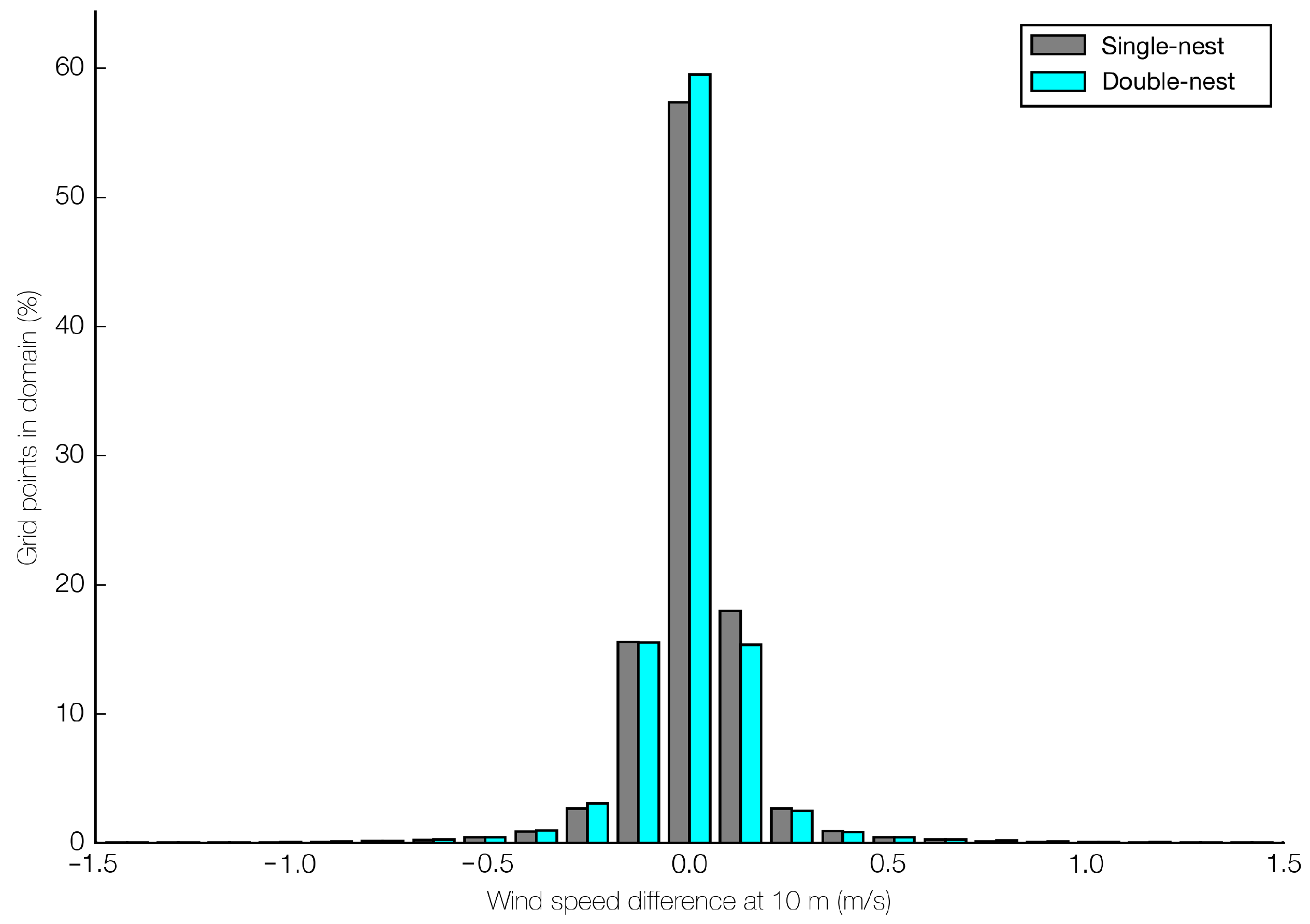
We use the Weather Research and Forecasting (WRF; Powers et al. [27]) version 3.5 to create the ensemble simulations. We initialize our simulations with the p09 member of the 11-member Global Ensemble Forecast System Reforecast dataset (GEFS/R2; Hamill et al. [28]) initialized at 0000 UTC 15 August 2013 (i.e., the MCS of interest is roughly 21 h into the simulation). Motivated by the desire to simulate a bowing MCS in all members, we used a SKEB scheme to generate perturbations, and a constant IC/LBC dataset and parameterization suite that performed well in preliminary testing (also see [2]). The SKEB scheme was developed in response to excessive kinetic energy dissipation near the truncation scale of NWP models [23,24], and adapted for WRF in Berner et al. [25]. While we use SKEB to increase the signal-to-noise ratio of our grid-spacing experiment, its use may result in a resulting bias of the ensemble mean. As described in Berner et al. [29], a simple stochastic scheme can push a non-linear model from a uniform or Gaussian distribution into a non-Gaussian one (e.g., asymmetric bimodal), biasing the mean state. However, we submit that perturbations from SKEB shift the simulations closer to the real-life attractor, and any shift of the mean corresponds to a convergence to a realistic state (albeit not necessarily the observed state at the given time). In any case, we find there is no obvious systematic bias introduced by the SKEB scheme before convective initiation: Figure 2 shows the distribution of 10-m wind-speed point-wise differences between the control (no-SKEB) and first ensemble member, after 3 h of simulation, for both ensembles. This quasi-Gaussian distribution is general to other ensemble members, variables (2-m temperature and mixing ratio), and bin sizes, and hence supports the deployment of SKEB as a variance generator in the present study.
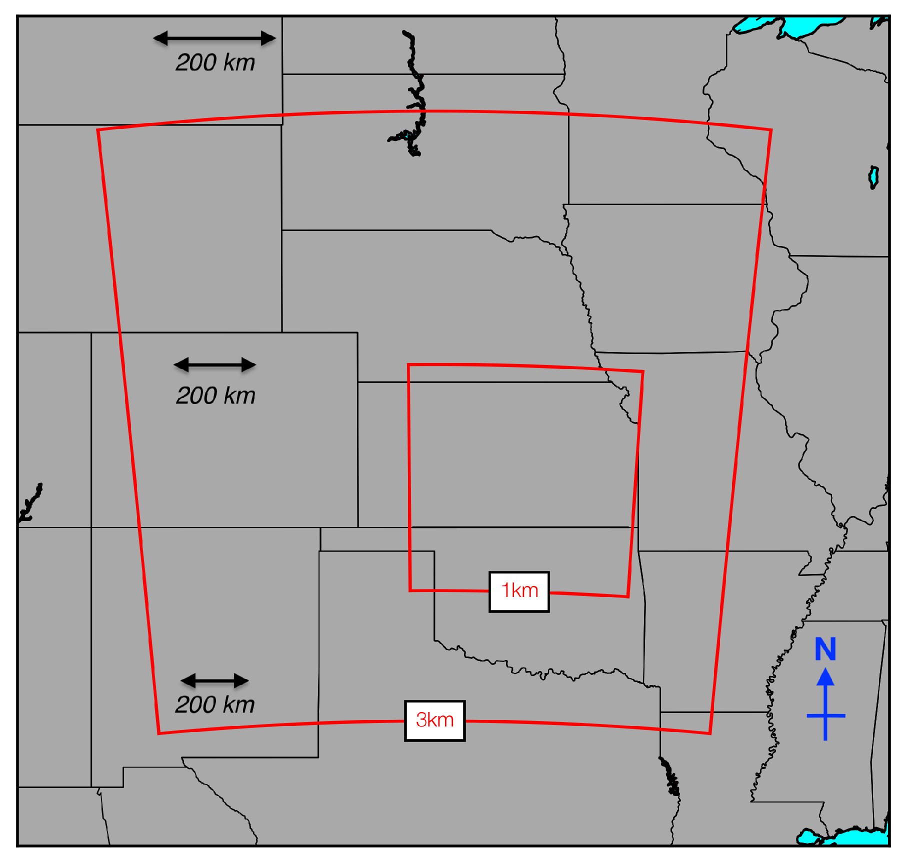
We used Thompson 1.5-moment microphysics, after preliminary testing showed it produced a MCS most similar to that observed [2]. Sensitivity of the MCS to microphysics parameterizations is substantial (e.g., [13]), but outside the scope of the present study. Other parameterizations are listed in Table 1. The single-nest 3-km EPS has eleven members: the control (with no SKEB scheme) and ten SKEB-perturbation members (s01–s10). The domain locations are labeled in Figure 3. Each perturbation member uses a different randomness seed to generate the backscatter pattern. The double-nest (3-km, 1-km) EPS uses an identical 3-km parent domain but with a two-way-feedback nested 1-km domain (Figure 3). The double-nest ensemble also has eleven members: the control and ten SKEB-perturbation members (s11–s20). The seeds across both EPS are unique. The two-way feedback was chosen to allow direct comparison between the two 3-km domains in the area in which the MCS developed. Each nest uses a timestep (in seconds) set to 2 Δ x (i.e., 6 s for the 3-km nest and 2 s for 1-km), after preliminary testing revealed larger timesteps incurred instability in the simulation. Lateral boundary conditions are updated every 3 h on the 3-km grid.

Verification and Spread

In addition to traditional gauges of ensemble spread, such as standard deviation at the Δ x scale, we implement a score that instead filters the simulation grids into objects (i.e., thunderstorms). The common 3-km grids allow use of such object-based skill scores to evaluate the ensemble spread and performance, without employing an interpolation or filtering step. We use a slightly modified version of the Structure–Amplitude–Location (SAL) method [30,31]. The original method was formulated for precipitation fields, and identifies objects (i.e., coherent structures that meet a strength threshold) in both simulations and observations. The simulation is then penalized according to normalized differences as follows:
  • Structure (S), between −2 and +2. A positive value indicates simulated objects are too large and/or too flat;
  • Amplitude (A), between −2 and +2. A positive value indicates the simulation has overestimated the domain-averaged variable (precipitation, reflectivity, etc.);
  • Location (L), between 0 and +2. A positive value indicates a displacement of simulated objects from those observed.
Our modification uses simulated and observed composite reflectivity instead of accumulated precipitation. We obtained composite NEXRAD Level III radar reflectivity from the Iowa State University [32]. Before reaching the archives, Base Reflectivity product data are composited with the GEMPAK program nex2img, after which false echoes are removed after comparison with the Net Echo Top product. Total absolute SAL (taSAL) is computed as follows:
taSAL = | S | + | A | + | L |
and varies between 0 (perfect forecast) and 6. The three components are combined this way in the absence of strong evidence to suggest otherwise, though unequal weightings are used in similar schemes (e.g., Method for Object-Based Diagnostic Evaluation; [33]). To gauge each EPS’s ability to capture the MCS structure, we take the median ensemble member (instead of the unphysical ensemble mean) to represent each EPS. This is done by ranking all ten perturbation members by their taSAL score, and taking the taSAL value halfway between the fifth and sixth most skillful members.
Objects are identified by masking the reflectivity field below a given dB Z threshold, and in our modification, we include objects only when they comprise a given number of gridpoints that exceed a size threshold (known as its footprint). As SAL was originally designed for a smoothed accumulated precipitation field, suitable footprint and threshold values were tested for instantaneous reflectivity fields. Values of 15–30 dBZ and 100–500 gridpoints (900–4500 km 2 in area) were relatively robust to small changes in these parameters. Above 30 dBZ and 500 gridpoints, there was substantial sensitivity to changes in threshold and footprint, due to a smaller sample size of objects at a given time and across the simulation period. High thresholds above 30 dBZ often created rapid increases in SAL from hour to hour as objects ‘appeared’ as they grew critically large. Conversely, much smaller thresholds and footprints captured too much signal from stratiform precipitation, which detracts from the focus on intense bow-echo convection in the simulation. Ultimately, the 15 dBZ threshold and 200 gridpoint footprint provided a robust compromise, and is used in the following text to estimate spread and skill in the ensemble simulations. Further discussion of the use of SAL to evaluate reflectivity forecasts can be found in Lawson and Gallus [31].

3. Results

3.1. Sensitivity of Structure to Δ x

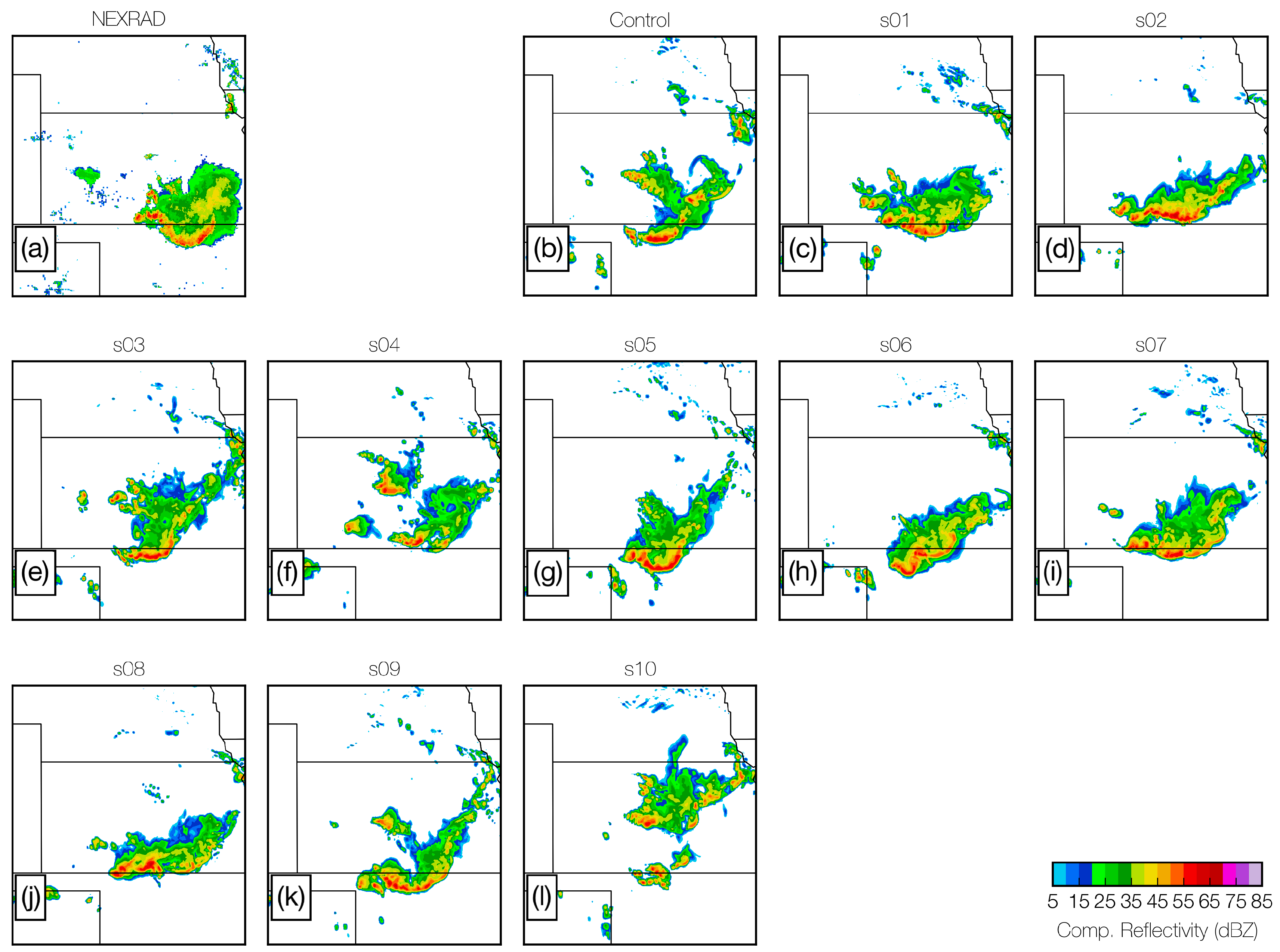
In the single-nest EPS, convective initiation occurs at the same time as in observations (2000 UTC on Day 1; not shown). Between 2100 UTC on Day 1 and 0600 UTC on Day 2, a spectrum of single-nest solutions—ranging from a collection of cells to a bow echo—are in contrast to the observed line of convection. The simulated MCSs in single-nest members generally lag ∼75 km behind the observed system in its southward progression. By 0600 UTC on Day 2, most single-nest members have captured the bow echo in Oklahoma.
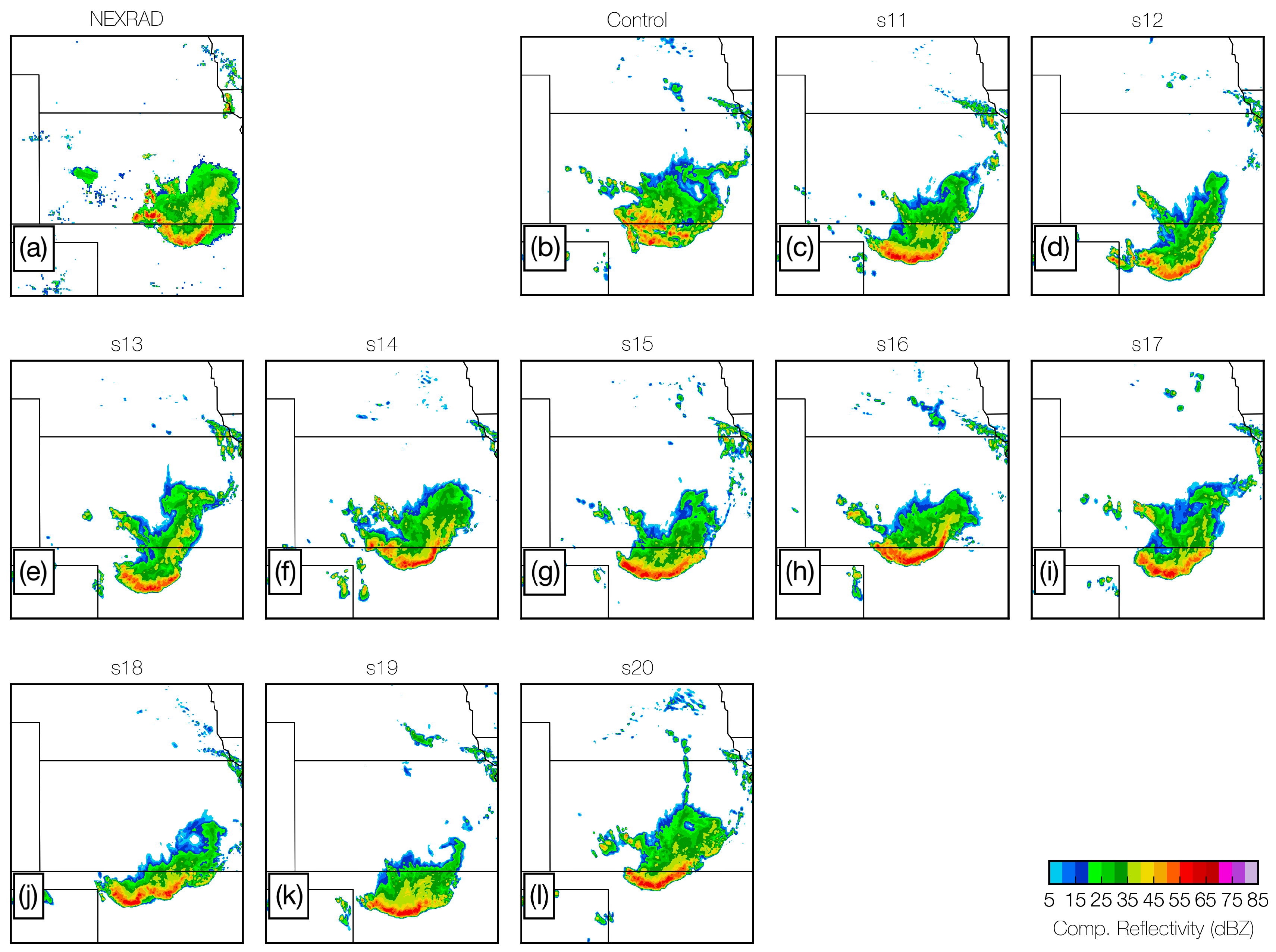
The double-nested (3-km/1-km) EPS has more inter-member agreement by 2100 UTC on Day 1 than in the single-nest EPS, with all members creating an MCS in a similar location to the observed system. At 0000 UTC on Day 2, all members have a bow echo, but it is too large in the zonal direction. In contrast to the single-nest EPS, the bow echoes simulated in double-nest members are co-located with, or in advance (to the south) of, the observed system throughout the lifetime of the system (2100 UTC–0600 UTC). At 0300 UTC on Day 2, almost all members reproduce the observed system, with approximately correct radii of curvature and lengthscale. In general, double-nest EPS members resemble the observed system better than members in the single-nest EPS, but accelerate the MCS too quickly. The following subsection now analyzes whether this translates to better object-based performance.

3.2. Sensitivity of Spread and Skill to Δ x

Following Tennekes [34], we may expect more spread within the double-nest EPS due to higher sensitivity of mesoscale processes to small perturbations when Δ x is decreased. Computation of standard deviation in preliminary work (performed on the 3-km grid) across multiple sensible weather variables (including 2-m temperature, 10-m wind; not shown) shows that ensemble uncertainty is similar in both ensembles until around 26 h (0200 UTC on Day 2). After this, standard deviation in the single-nest EPS grows faster and remains larger than in the double-nest EPS until the end of the simulation. This signal is seen in Figure 4 and Figure 5 as a larger spread, by eye, in the positioning of the bow-echo system in the single-nest EPS. The above method uses a point-wise variance estimation at the Δ x scale, and is therefore not appropriate for assessing the spread of structural solutions. Hence, we implement an object-based score (SAL) to add weight to subjective conclusions reached herein.
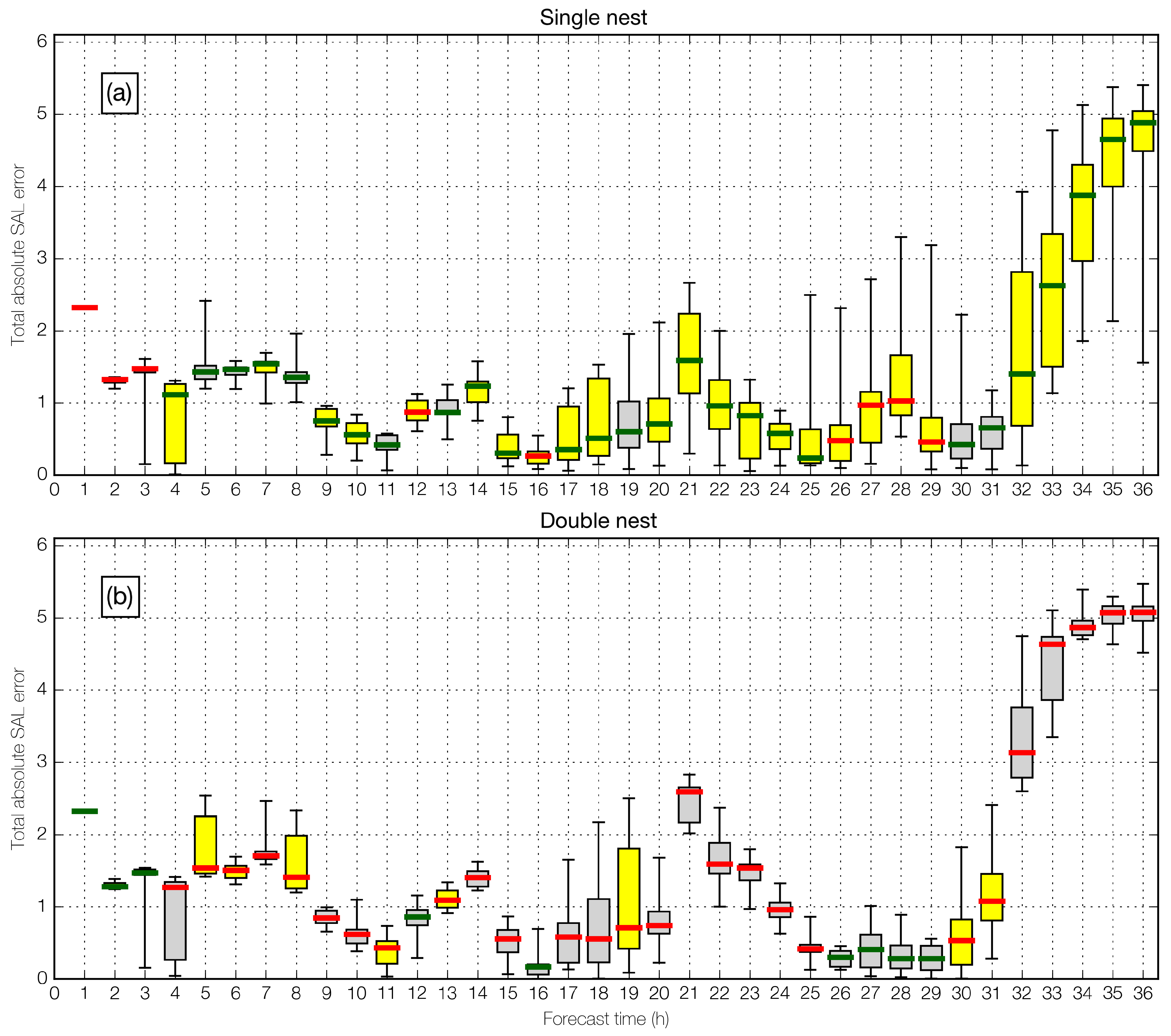
Figure 6 shows the median, interquartile range, and spread of the EPS for both the single- and double-nested experiments. At each forecast time shown (every 60 min), the two EPSs are compared. The smaller median value is colored green (i.e., a better forecast) while the larger is colored red. Likewise, the larger interquartile range is colored yellow (more variation between ensemble members, ignoring outliers), while the smaller spread is colored gray.
Figure 6 shows the single-nest EPS has a lower median (better forecast) than the double-nest EPS for ∼75% of the time periods. The single-nest EPS also has more variation in taSAL score (76% of times, neglecting the first three hours with little convective activity). The exception to this pattern occurs between 0200 UTC and 0500 UTC on Day 2, inclusive (26 h to 29 h forecast hours). By this time the MCS, having grown upscale from isolated cells, displays a bowing structure, and there is good agreement between double-nest EPS members (but not in the single-nest EPS). The poor performance of the double-nest EPS before 0200 UTC may be related to its overly hasty development, and excessive west–east length, of the bow echo. After this time, however, the double-nest EPS has a lower median until 0500 UTC, matching its subjectively better reflectivity fields. Throughout the entire period, there is little correlation between taSAL variance and median (skill) at each hour. Further, the S and A components are comparable in magnitude throughout, whereas L is an order of magnitude smaller. Hence, we complement the L-component assessment of location error with centroid tracking in later subsections.

3.3. Sensitivity of System Speed to Δ x

We now investigate the difference in development and acceleration of the bow echo as Δ x decreases. We subjectively chose representative members within both ensembles by calculating taSAL for each member, and choosing the median member at 0000 UTC (as the bow echo is reaching maturity in observations). The single-nest (s06) and double-nest (s12) members are hence discussed in the following section. In the following analysis, cold-pool strength is depicted by the density potential temperature perturbation field ( θ ρ ), as in Markowski and Richardson [35]. It is computed by subtracting density potential temperature θ ρ from the domain mean at each timestep, where
θ ρ = θ ( 1 + 0.61 r v r h )
and where r v and r h are the mixing ratios of water vapor and all other hydrometeor species, respectively. Figure 7 presents observed and simulated composite reflectivity, and simulated θ ρ to depict the near-surface cold pool, at three times: 21 h, 24 h, and 27 h simulation time. At 21 h, the cold pool is ∼50 km farther south in the double-nest member, but the peak magnitude of θ ρ is similar in both members at this time (∼12 K). Three hours later, the double-nest member’s cold pool is substantially more developed in areal coverage and magnitude, and has progressed farther south. Three hours later still, as the bow echo weakens, there is little difference in magnitude between the two simulations, though the double-nest member leaves a more pronounced wake of cold air. Values have also decreased, however, as θ ρ has a strong diurnal dependence. Despite the more distinctive bow-echo structure in the double-nest member, the bow-echo location in the single-nest member is closer to that observed.
Figure 8 shows the progression of the MCS-object centroids with time. This was done by taking the reflectivity objects identified using the SAL technique (and the same parameters used herein), and tracking the location of the object’s centroid every 20 min (the output frequency). As in Figure 7, the mean ensemble system speed is higher in the double-nest EPS, denoted by the y-position of the timestamp labels at a given time. The spread of bow-echo centroid locations is initially large in the double-nest EPS, but becomes more similar to the single-nest over time. For instance, contrast the two clusters of centroids at 0400 UTC in the single-nest EPS to the more compact single group in the double-nest EPS.
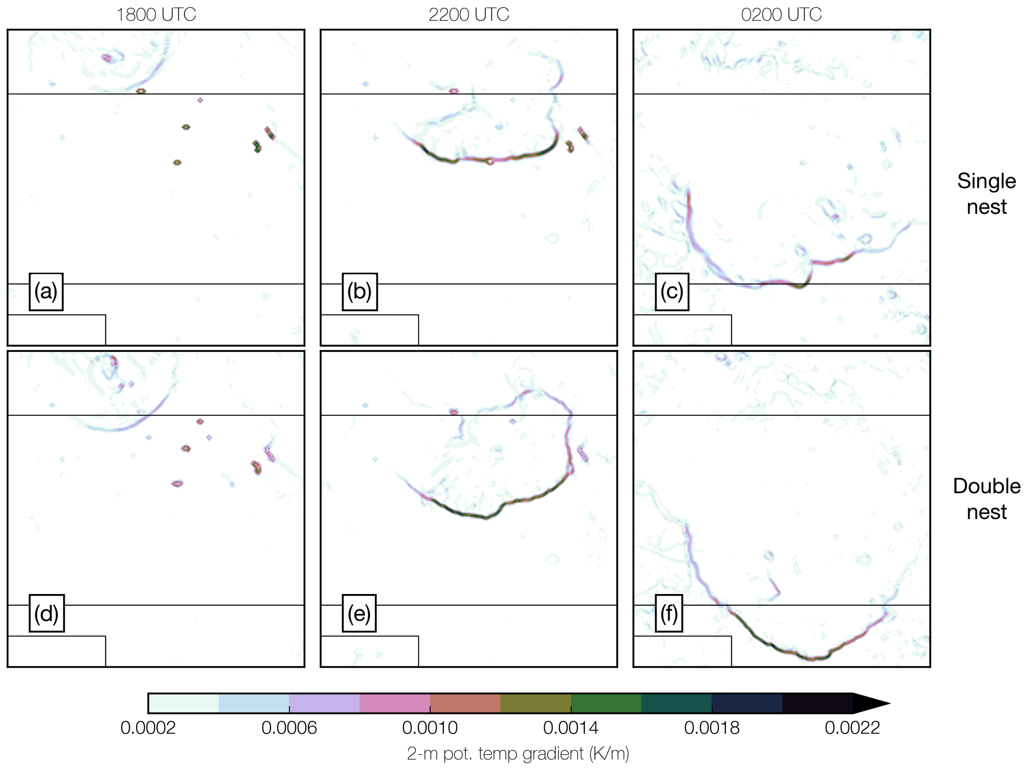
We now use the same median members as in Figure 7 to investigate the bow echo propagation mechanism. The movement of a cold pool is related to its strength (perturbation of density or 2-m potential temperature) and hence pressure gradient. Prior to MCS development at 1800 UTC on Day 1, the gradient of 2-m potential temperature is similar (∼0.75 × 10 3 K m 1 ) in the single- and double-nest members (Figure 9a,d). Four hours later, the cold pool has moved farther south in the double-nest member (Figure 9b,e), marked at its leading edge by larger values of potential-temperature gradient (∼2 × 10 3 K m 1 ) than in the single-nest member. Four hours later still, there is ∼125 km meridional difference between single- and double-nest cold-pool leading edges (Figure 9c,f), and the double-nest leading edge is associated with a temperature gradient (2 × 10 3 K m 1 ) double in magnitude of the gradient in the single-nest member. An increased gradient along the double-nest median-member cold-pool leading edge is also seen in surface pressure (not shown).
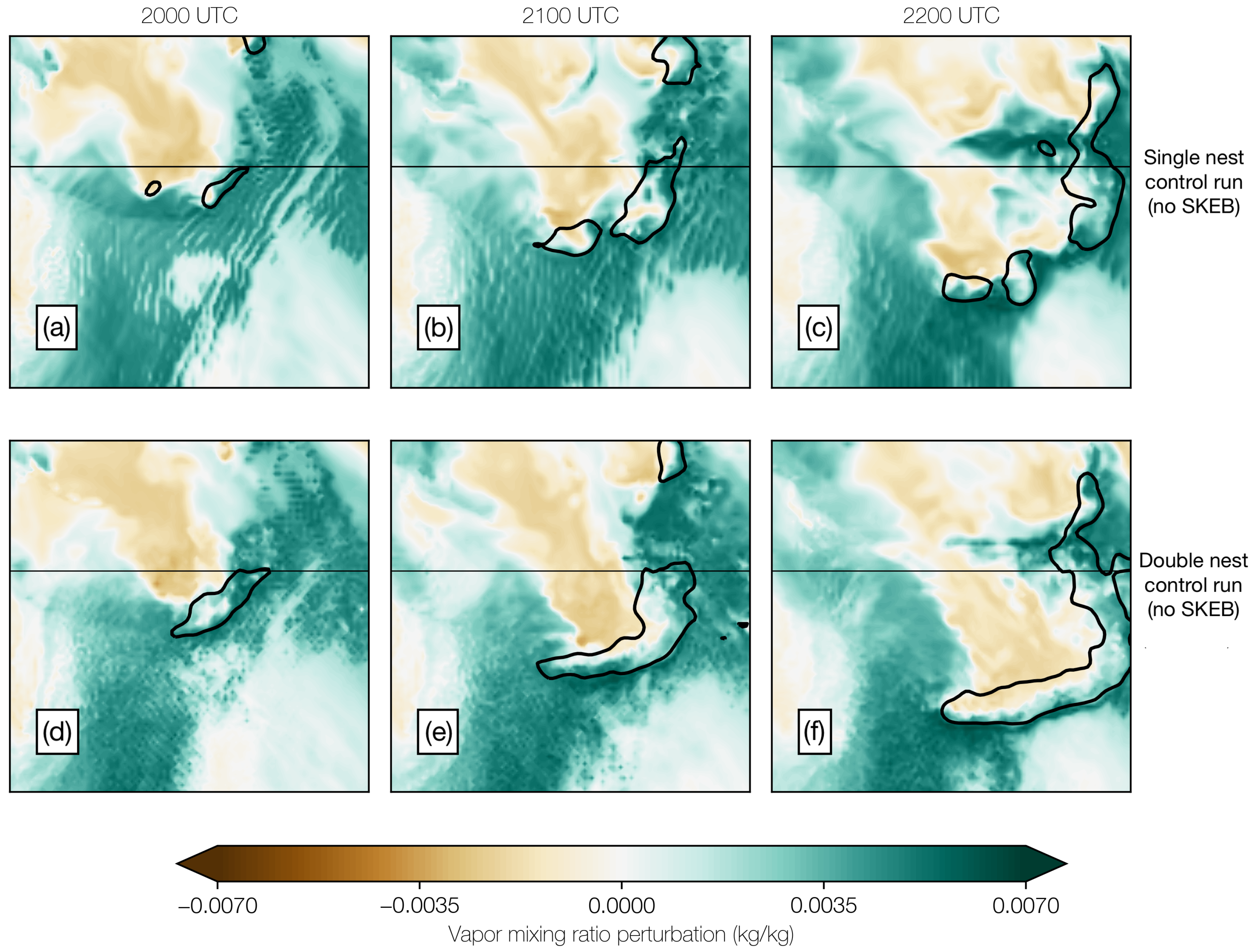
The faster movement in the double-nested simulation is similar to behavior documented by Weisman et al. [36]. In their simulations of linear MCSs—with Δ x ranging from 1 km to 12 km—the higher-resolution simulations better developed a feed of low- θ e air. They also found a slower system evolution on coarser grids, and that MCSs developing near MCVs (such as in the present study) may be more predictable due to associated dynamical balance. To gauge solely the sensitivity of system speed to resolution, we compare the control members from single- and double-nest experiments; the only difference between the two simulations is the addition of the inner nest (i.e., no SKEB scheme is active). Figure 10 shows perturbation water-vapor mixing ratio ( q ) at 800 hPa at three times, for the two control members. The 35-dBZ simulated composite reflectivity contour, smoothed with a 9-km Gaussian filter, is overlaid for reference. At 2000 UTC on Day 1, there is little difference between the two simulations (cf. panel a,d). The rear-inflow jet is associated with drier air behind the burgeoning moist convection. As the system intrudes farther into the region covered by the 1-km nest (cf. panel b with e), the drier air in the double-nest run penetrates farther south than in the single-nest run, and is associated with a more coherent, bowing segment of high reflectivity. This is even more pronounced by 2200 UTC (cf. panel c with f). This bowing also requires descent of strong winds aloft; such downdrafts may themselves be sensitive to resolution, given that the strength of convective downdrafts is related to microphysical processes (condensate loading, evaporation, and so on).
Cross-sections perpendicular to the bow-echo apex are shown in Figure 11 at 2100 UTC on Day 1 (cf. Figure 10b,e); winds perpendicular to the cross-section transect are contoured and q is color-filled. Note the cross-sections (Figure 11a,c) were averaged 6 km (two grid points) in each direction normal to the cross-section transect to improve representivity. During preliminary testing, the averaging was varied, but did not substantially change the conclusions. While more smoothing increases the representivity of Figure 11, some finer details are lost. The double-nest control-run cross-section (Figure 11c) shows winds over 20 m s 1 and low q air descending and feeding into the rear of the bow echo; this is absent in the single-nest run (Figure 11a), and corroborates the latitude–longitude cross-section at 800 hPa in Figure 10. Taking a similar horizontal slice at 800 hPa in the wind field for both single- and double-nest members (Figure 12), we find a more coherent rear-inflow jet in the latter. Whereas strong winds do occur along the bow-echo leading edge in the former (southwest of the cross-section transect), associated with cellular development (cf. Figure 11b), they are rather disconnected from the channel of wind farther north. In fact, there is around 30 m s 1 difference in wind vectors associated with the rear-inflow jet (not shown). In summary, the nested 1-km domain appears to have an enhanced and more coherent rear-inflow jet, which in turn increases evaporational cooling. The resultant cold pool is stronger, and accelerates faster due to increased surface pressure gradients. Note that bow echoes move due to the buoyancy gradient [35], and are not “advected” along by the winds, and hence we should not necessarily expect rear-inflow jet speed to correlate with system speed.
But why may the rear-inflow jet be stronger with a smaller Δ x ? The perimeter of a two-dimensional fractal object (i.e., infinitely complex regardless of zoom level) is sensitive to the measuring interval [37], and similarly for surface area of three-dimensional objects. Stronger cold pools in higher-resolution simulations are related to evaporation of falling precipitation [18], enhancing the convective downdraft at lower levels. Higher horizontal resolution yields a larger surface area of clouds (which are fractal), and hence the increased interface of dry air and cloud water content may add to this precipitation evaporation, and hence yield a stronger cold pool.

3.4. Sensitivity of System Speed to Skeb

The region in the wake of an MCS leading edge is turbulent [38], represented herein by the descending drier air in Figure 11; hence, entrainment may increase in SKEB members, as the SKEB scheme increases turbulence through the injection of kinetic energy into resolved scales. As discussed earlier, if this is indeed the case, it represents a convergence towards a more realistic system due to the reduced dissipation of kinetic energy at the truncated scale.
We find the control (no-SKEB) member of the double-nest EPS has the weakest rear-inflow jet at 2300 UTC on Day 1 out of all its members (seen in 800-hPa mixing-ratio perturbation field; not shown), and the least coherent and slowest-moving bow echo until 0330 UTC. This connection between the rear-inflow jet and bow-echo speed is similar to results in the previous subsection. However, in the single-nest ensemble, the control member does not have the slowest bow echo. As such, further ensemble simulations are needed to address the link between SKEB perturbations and MCS speed.

4. Summary and Conclusions

Two Δ x = 3 km ensemble simulations of a bowing MCS (or bow echo), one with a nested 1-km domain, have addressed the hypothesis that a smaller Δ x increases the uncertainty within an ensemble. An increase of spread in the double-nest (3-km/1-km) simulation does not occur, as measured by standard deviation of various fields on the 3-km grid (at the Δ x scale). Further analysis of reflectivity objects via the SAL methodology, in fact, suggests:
  • The spread of taSAL scores is larger in the single-nest ensemble. This disputes the hypothesis that spread increases as Δ x decreases;
  • Skill is higher in the single-nest ensemble, as measured objectively using the ensemble median; however, MCS structure in simulated reflectivity is subjectively more realistic in the double-nest ensemble, as expected from the nesting of a higher-resolution domain;
  • While both taSAL-measured spread and skill are higher in the single-nest ensemble overall, there is a lack of correlation between the two over the hourly forecast times, in both ensembles.
The reduced spread of MCS evolutions in the double-nest (3-km/1-km) EPS may be related to the stronger cold pools, and hence stronger mesoscale forcing, in the higher-resolution nest. The faster movement in the double-nested (3-km/1-km) simulation is likely driven by a stronger surface-based cold pool, which occurs with a stronger rear-inflow jet. We propose this may be related to the fractal nature of clouds and turbulence, as follows: in a higher-resolution simulation, a given cloud object will have larger surface area (i.e., its fractal dimension increases). More resolved turbulence also increases dry-air entrainment. These two factors increase the interfacing of dry air with cloud water content, increasing evaporation. This strengthens the surface-based cold pool and the corresponding pressure gradient behind and ahead of the MCS’s leading edge. In our simulations, the MCS surges ∼100–200 km farther south at its mature stage (0300 UTC on Day 2) than in coarser simulations. However, there may well be further competing mechanisms that prevents further MCS acceleration as resolution decreases, as seen in [21]. In summary, because entrainment is likely underestimated on the single-nest (3-km) grid through poorly resolved kinematic system structure [39], this compounds the underestimation also present in subgrid parameterization. The kinematic structure of the MCS is better captured on the 1-km grid, reducing the underestimation of entrainment, but sub-grid error is still substantial. It may be that the faster system speed at 1-km is related to this reduction of grid-scale error, rather than increased realism in a higher-resolution simulation.
We note that location error in SAL is a function of the domain size (i.e., it is normalized by the domain diagonal, as this is the largest magnitude of error that can occur). Because the location errors are small relative to domain size, but still substantial given potential point forecasts for the end user, the taSAL score may not be appropriate for evaluating spread and skill depending on the end user’s sensitivity to location error. The single-nest ensemble does have more location error, by eye, in reflectivity fields; however, despite the low weight of the location component, this ensemble has more taSAL spread than the nested ensemble regardless (i.e., taSAL is a conservative estimate). Further work into bowing MCS evolution in EPSs should consider the probabilistic distribution of solutions by using an appropriate score that preserves the ensemble-output estimates of uncertainty (e.g., [40,41,42]).
The larger bow-echo speed and faster rear-inflow jet winds, when resolution is increased, is also seen in the authors’ preliminary simulations of two bowing linear MCSs (unpublished), and in a similar study [43]. We show little advantage, in terms of spread and skill, for the O(30) increase in computer power to reduce Δ x from 3 km to 1 km. At the least, our results suggests caution against the backdrop of the grid-spacing arms race regarding bow-echo and MCS prediction. In addition, the spread of convective mode solutions is not increased by increasing resolution, hence substantial increase in ensemble membership may not be required to maintain a good sampling within a higher resolution ensemble. It remains an open question whether the stronger bowing MCS and lower skill of the double-nest experiment is general to other cases and ensemble configurations. Further, more analysis of cloud surface area is required to test impact of fractal dimension on entrainment. These questions, and the sensitivity of bow-echo speed to SKEB perturbations, should be the subject of further work.

Author Contributions

Conceptualization, J.R.L. and W.A.G.J.; methodology, J.R.L.; software, J.R.L.; validation, J.R.L., W.A.G.J., and C.K.P.; formal analysis, J.R.L. and W.A.G.J.; investigation, J.R.L. and W.A.G.J.; resources, J.R.L.; data curation, J.R.L.; writing—original draft preparation, J.R.L.; writing—review and editing, J.R.L., W.A.G.J., and C.K.P.; visualization, J.R.L.; supervision, W.A.G.J. and C.K.P.; project administration, W.A.G.J.; funding acquisition, W.A.G.J. All authors have read and agreed to the published version of the manuscript.

Funding

Research supported by grants NSF-AGS1222383 and NSF-AGS1624947. Funding was also provided by NOAA/Office of Oceanic and Atmospheric Research under NOAA-University of Oklahoma Cooperative Agreement NA11OAR4320072, U.S. Department of Commerce.

Acknowledgments

This paper is in memory of Ray Arritt, who contributed early reviews that improved the manuscript. The authors also thank, in alphabetical order, for discussions and assistance during this study: Judith Berner, Jeffrey Duda, David Flory, Jonathan Flowerdew, Matthew Flourney, Anna Ghelli, Lee Grenci, William Gutowski, Daryl Herzmann, Makenzie Krocak, Anne McCabe, David Schultz, Brian Squitieri, Richard Swinbank, Ryan Torn, Andy Vanlooke, Louis Wicker, and Xiaoqing Wu. We thank the editor and four anonymous reviewers for strengthening the manuscript during review. In addition, comments from two anonymous reviewers of a previous incarnation of the manuscript were appreciated. All computations were performed with Python packages numpy and python-netcdf4, and figures were generated with Python packages matplotlib and basemap.

Conflicts of Interest

The authors declare no conflict of interest. In addition, those funding the project had no role in the design of the study; in the collection, analyses, or interpretation of data; in the writing of the manuscript, or in the decision to publish the results.

Abbreviations

The following abbreviations are used in this manuscript:
NWPNumerical weather prediction
MCSMesoscale convective system
MCVMesoscale convective vortex
GEFS/R2Global Ensemble Forecasting System, Reforecast version 2
WRFWeather Research and Forecast (model)
Δ x Horizontal grid spacing

References

  1. Snively, D.V.; Gallus, W.A. Prediction of Convective Morphology in Near-Cloud-Permitting WRF Model Simulations. Weather Forecast. 2014, 29, 130–149. [Google Scholar] [CrossRef] [Green Version]
  2. Lawson, J.; Gallus, W.A., Jr. On Contrasting Ensemble Simulations of Two Great Plains Bow Echoes. Weather Forecast. 2016, 31, 787–810. [Google Scholar] [CrossRef]
  3. Durran, D.R.; Weyn, J.A. Thunderstorms Do Not Get Butterflies. Bull. Am. Meteorol. Soc. 2016, 97, 237–243. [Google Scholar] [CrossRef]
  4. Lorenz, E.N. Deterministic Nonperiodic Flow. J. Atmos. Sci. 1963, 20, 130–141. [Google Scholar] [CrossRef] [Green Version]
  5. Stensrud, D.J.; Bao, J.W.; Warner, T.T. Using initial condition and model physics perturbations in short-range ensemble simulations of mesoscale convective systems. Mon. Weather Rev. 2000, 128, 2077–2107. [Google Scholar] [CrossRef]
  6. Buizza, R.; Milleer, M.; Palmer, T.N. Stochastic representation of model uncertainties in the ECMWF ensemble prediction system. Q. J. R. Meteorol. Soc. 1999, 125, 2887–2908. [Google Scholar] [CrossRef]
  7. Leutbecher, M.; Palmer, T.N. Ensemble forecasting. J. Comput. Phys. 2008, 227, 3515–3539. [Google Scholar] [CrossRef]
  8. Whitaker, J.S.; Loughe, A.F. The Relationship between Ensemble Spread and Ensemble Mean Skill. Mon. Weather Rev. 1998, 126, 3292–3302. [Google Scholar] [CrossRef] [Green Version]
  9. Lorenz, E.N. The predictability of a flow which possesses many scales of motion. Tellus 1969, 21, 289–307. [Google Scholar] [CrossRef]
  10. Palmer, T.N.; Döring, A.; Seregin, G. The real butterfly effect. Nonlinearity 2014, 27, R123. [Google Scholar] [CrossRef]
  11. Potvin, C.K.; Murillo, E.M.; Flora, M.L.; Wheatley, D.M. Sensitivity of Supercell Simulations to Initial-Condition Resolution. J. Atmos. Sci. 2017, 74, 5–26. [Google Scholar] [CrossRef] [Green Version]
  12. Schwartz, C.S.; Sobash, R.A. Revisiting sensitivity to horizontal grid spacing in convection-allowing models over the central–eastern United States. Mon. Weather Rev. 2019, 147, 4411–4435. [Google Scholar] [CrossRef]
  13. Thielen, J.E.; Gallus, W.A. Influences of Horizontal Grid Spacing and Microphysics on WRF Forecasts of Convective Morphology Evolution for Nocturnal MCSs in Weakly Forced Environments. Weather Forecast. 2019, 34, 1495–1517. [Google Scholar] [CrossRef]
  14. Sobash, R.A.; Schwartz, C.S.; Romine, G.S.; Weisman, M.L. Next-Day Prediction of Tornadoes Using Convection-Allowing Models with 1-km Horizontal Grid Spacing. Weather Forecast. 2019, 34, 1117–1135. [Google Scholar] [CrossRef]
  15. Sobash, R.A.; Schwartz, C.S.; Romine, G.S.; Fossell, K.R.; Weisman, M.L. Severe Weather Prediction Using Storm Surrogates from an Ensemble Forecasting System. Weather Forecast. 2016, 31, 255–271. [Google Scholar] [CrossRef]
  16. Potvin, C.K.; Flora, M.L. Sensitivity of Idealized Supercell Simulations to Horizontal Grid Spacing: Implications for Warn-on-Forecast. Mon. Weather Rev. 2015, 143, 2998–3024. [Google Scholar] [CrossRef]
  17. Berner, J.; Jung, T.; Palmer, T.N. Systematic Model Error: The Impact of Increased Horizontal Resolution versus Improved Stochastic and Deterministic Parameterizations. J. Clim. 2012, 25, 4946–4962. [Google Scholar] [CrossRef] [Green Version]
  18. Bryan, G.H.; Morrison, H. Sensitivity of a Simulated Squall Line to Horizontal Resolution and Parameterization of Microphysics. Mon. Weather Rev. 2012, 140, 202–225. [Google Scholar] [CrossRef]
  19. Squitieri, B.J.; Gallus, W.A. On the forecast sensitivity of MCS cold pools and related features to horizontal grid-spacing in convection-allowing WRF simulations. Weather Forecast. 2020, 35, 325–346. [Google Scholar] [CrossRef]
  20. Lebo, Z.J.; Morrison, H. Effects of Horizontal and Vertical Grid Spacing on Mixing in Simulated Squall Lines and Implications for Convective Strength and Structure. Mon. Weather Rev. 2015, 143, 4355–4375. [Google Scholar] [CrossRef]
  21. Varble, A.; Morrison, H.; Zipser, E. Effects of Under-Resolved Convective Dynamics on the Evolution of a Squall Line. Mon. Weather Rev. 2020, 148, 289–311. [Google Scholar] [CrossRef]
  22. Johnson, A.; Wang, X.; Kong, F.; Xue, M. Object-Based Evaluation of the Impact of Horizontal Grid Spacing on Convection-Allowing Forecasts. Mon. Weather Rev. 2013, 141, 3413–3425. [Google Scholar] [CrossRef]
  23. Mason, P.J.; Thomson, D.J. Stochastic backscatter in large-eddy simulations of boundary layers. J. Fluid Mech. 1992, 242, 51–78. [Google Scholar] [CrossRef]
  24. Shutts, G. A kinetic energy backscatter algorithm for use in ensemble prediction systems. Q. J. R. Meteorol. Soc. 2005, 131, 3079–3102. [Google Scholar] [CrossRef] [Green Version]
  25. Berner, J.; Ha, S.Y.; Hacker, J.P.; Fournier, A.; Snyder, C. Model Uncertainty in a Mesoscale Ensemble Prediction System: Stochastic versus Multiphysics Representations. Mon. Weather Rev. 2011, 139, 1972–1995. [Google Scholar] [CrossRef] [Green Version]
  26. Storm Prediction Center. Available online: http://www.spc.noaa.gov/products/md/2013/md1723.html (accessed on 1 March 2016).
  27. Powers, J.G.; Klemp, J.B.; Skamarock, W.C.; Davis, C.A.; Dudhia, J.; Gill, D.O.; Coen, J.L.; Gochis, D.J.; Ahmadov, R.; Peckham, S.E.; et al. The Weather Research and Forecasting Model: Overview, System Efforts, and Future Directions. Bull. Am. Meteorol. Soc. 2017, 98, 1717–1737. [Google Scholar] [CrossRef]
  28. Hamill, T.M.; Bates, G.T.; Whitaker, J.S.; Murray, D.R.; Fiorino, M.; Galarneau, T.J.; Zhu, Y.; Lapenta, W. NOAA’s second-generation global medium-range ensemble reforecast data set. Bull. Am. Meteorol. Soc. 2013, 94, 1553–1565. [Google Scholar] [CrossRef]
  29. Berner, J.; Achatz, U.; Batté, L.; Bengtsson, L.; Cámara, A.D.L.; Christensen, H.M.; Colangeli, M.; Coleman, D.R.B.; Crommelin, D.; Dolaptchiev, S.I.; et al. Stochastic Parameterization: Toward a New View of Weather and Climate Models. Bull. Am. Meteorol. Soc. 2017, 98, 565–588. [Google Scholar] [CrossRef] [Green Version]
  30. Wernli, H.; Paulat, M.; Hagen, M.; Frei, C. SAL—A novel quality measure for the verification of quantitative precipitation forecasts. Mon. Weather Rev. 2008, 136, 4470–4487. [Google Scholar] [CrossRef] [Green Version]
  31. Lawson, J.R.; Gallus, W.A. Adapting the SAL method to evaluate reflectivity forecasts of summer precipitation in the central United States. Atmos. Sci. Lett. 2016, 17, 524–530. [Google Scholar] [CrossRef]
  32. Iowa State University NEXRAD Composites. Available online: https://mesonet.agron.iastate.edu/docs/nexrad_composites/ (accessed on 1 December 2019).
  33. Davis, C.A.; Brown, B.G.; Bullock, R.; Halley-Gotway, J. The Method for Object-Based Diagnostic Evaluation (MODE) Applied to Numerical Forecasts from the 2005 NSSL/SPC Spring Program. Weather Forecast. 2009, 24, 1252–1267. [Google Scholar] [CrossRef] [Green Version]
  34. Tennekes, H. Turbulent Flow in Two and Three Dimensions. Bull. Am. Meteorol. Soc. 1978, 59, 22–28. [Google Scholar] [CrossRef]
  35. Markowski, P.; Richardson, Y. Mesoscale Meteorology in Mid-Latitudes; Wiley-Blackwell: Hoboken, NJ, USA, 2010; p. 407. [Google Scholar]
  36. Weisman, M.L.; Skamarock, W.C.; Klemp, J.B. The Resolution Dependence of Explicitly Modeled Convective Systems. Mon. Weather Rev. 1997, 125, 527–548. [Google Scholar] [CrossRef]
  37. Mandelbrot, B. How long is the coast of Britain? Statistical self-similarity and fractional dimension. Science 1967, 156, 636–638. [Google Scholar] [CrossRef] [Green Version]
  38. Droegemeier, K.K.; Wilhelmson, R.B. Numerical Simulation of Thunderstorm Outflow Dynamics. Part I: Outflow Sensitivity Experiments and Turbulence Dynamics. J. Atmos. Sci. 1987, 44, 1180–1210. [Google Scholar] [CrossRef] [Green Version]
  39. Adlerman, E.J.; Droegemeier, K.K. The Sensitivity of Numerically Simulated Cyclic Mesocyclogenesis to Variations in Model Physical and Computational Parameters. Mon. Weather Rev. 2002, 130, 2671–2691. [Google Scholar] [CrossRef] [Green Version]
  40. Gilleland, E. A New Characterization within the Spatial Verification Framework for False Alarms, Misses, and Overall Patterns. Weather Forecast. 2017, 32, 187–198. [Google Scholar] [CrossRef]
  41. Radanovics, S.; Vidal, J.P.; Sauquet, E. Spatial Verification of Ensemble Precipitation: An Ensemble Version of SAL. Weather Forecast. 2018, 33, 1001–1020. [Google Scholar] [CrossRef]
  42. Flora, M.L.; Skinner, P.S.; Potvin, C.K.; Reinhart, A.E.; Jones, T.A.; Yussouf, N.; Knopfmeier, K.H. Object-based verification of short-term, storm-scale probabilistic mesocyclone guidance from an experimentalWarn-on-Forecast system. Weather Forecast. 2019, 34, 1721–1739. [Google Scholar] [CrossRef]
  43. Squitieri, B.J.; Gallus, W.A., Jr. On the Acceleration of Nocturnal Mesoscale Convective Systems in Simulations with Increased Horizontal Grid Spacing. In Proceedings of the 97th AMS Annual Meeting, Seattle, WA, USA, 22–26 January 2017. [Google Scholar]
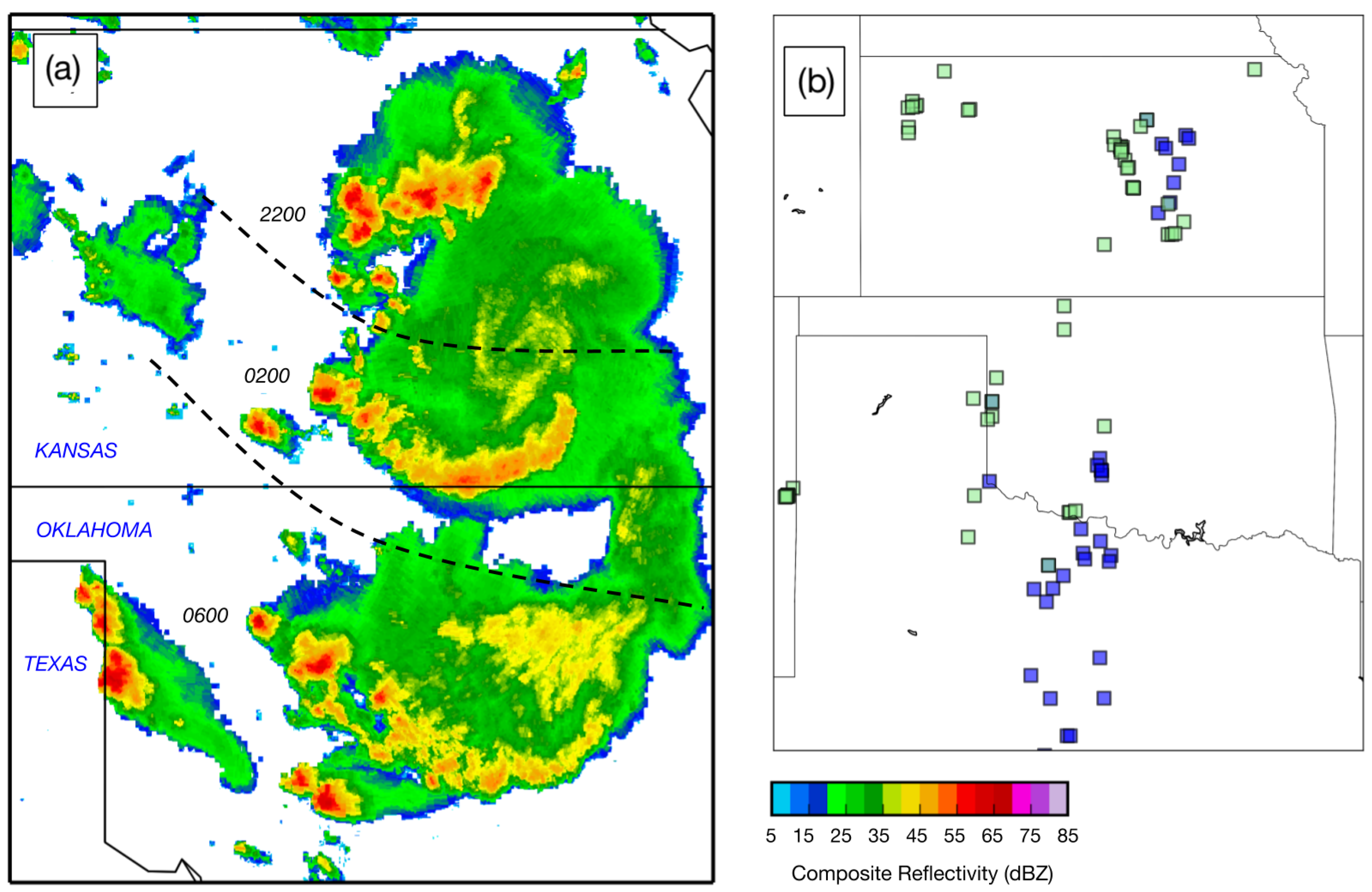
Figure 1. Overview of the bowing MCS of interest: (a) time-composited image of observed composite radar reflectivity at three times (2200 UTC Day 1, 0200 UTC Day 2, and 0600 UTC Day 2), as the system moved south. Dashed lines roughly delineate the three times from which reflectivity is drawn; and (b) National Centers for Environmental Information storm data for all wind reports exceeding 25 m s 1 (50 kt; in blue) and hail reports exceeding 2.54 cm (1 in; in green).
Atmosphere 11 00384 g001
Figure 2. Distribution of 10-m wind-speed point-wise differences between the control (no-SKEB) and first ensemble member after 3 h of simulation, for both ensembles (see key). A positive value indicates that SKEB has increased the wind speed at a given gridpoint. The y-axis indicates percentage of total grid points.
Atmosphere 11 00384 g002
Figure 3. Domains used in the present study. The single-nest ensemble uses the 3-km domain; the double-nest ensemble nests the 1-km domain inside the 3-km domain.
Atmosphere 11 00384 g003
Figure 4. Thumbnails of observed (a) and simulated (bl) composite reflectivity, valid at 0300 UTC 16 August 2013 (27 h simulation time), for the single-nest EPS. Reflectivity is contour-filled in dBZ according to the scale.
Atmosphere 11 00384 g004
Figure 5. As Figure 4, but for the double-nest (3-km/1-km) EPS.
Atmosphere 11 00384 g005
Figure 6. Box plot of total absolute SAL (taSAL) for the (a) single- and (b) double-nested EPSs. Features shown include median (linearly interpolated; horizontal line), interquartile range (box), and spread of the whole ensemble (whiskers). The lower median (better forecast) at each time is colored green, while the higher median is red. The larger interquartile range at each time is colored yellow; the smaller is colored gray.
Atmosphere 11 00384 g006
Figure 7. Observed composite reflectivity (leftmost column), and simulated fields of composite reflectivity (second and third column from left) and density potential temperature perturbation (two rightmost columns) from total absolute SAL median single- and double-nest EPS members. Fields are valid at 2100 UTC on Day 1 (ae), 0000 UTC on Day 2 (fj), and 0300 UTC on Day 2 (ko). Times are listed on the right as hours since initialization.
Atmosphere 11 00384 g007
Figure 8. Paths taken by the centroids of the MCS in each ensemble member for the single- (left) and double-nest (right) EPSs between 2200 UTC on Day 1 (22 h) and 0800 UTC on Day 2 (32 h). The centroid position is marked every two hours for each ensemble member by a dot. The color corresponds to the labeled time stamps, which are positioned at the ensemble-mean north-south position. Hence, locational spread is represented by a larger distance between dots of the same color.
Atmosphere 11 00384 g008
Figure 9. Potential temperature at 2 m (color-filled) taken from total absolute SAL median single- (s06; ac) and double-nest (s12; df) EPS members. Fields shown at (a,d) 18 h, (b,e) 22 h, and (c,f) 26 h simulation time. States shown in each panel, from north to south, are Nebraska, Kansas, Oklahoma, and (the panhandle of) Texas.
Atmosphere 11 00384 g009
Figure 10. Perturbation water-vapor mixing ratio at 800 hPa (color-filled) taken from control members of single-nest (ac) and double-nest (df) experiments. Black lines contour the 35 dBZ composite reflectivity field, smoothed with a 9-km Gaussian filter, for reference. Fields shown at 20 h (a,d), 21 h (b,e), and 22 h (c,f) simulation time. States shown in each panel are Nebraska (upper) and Kansas (lower), separated by the thin horizontal black line.
Atmosphere 11 00384 g010
Figure 11. Cross-sections at 2100 UTC on Day 1: (a,c) height against horizontal distance in the water mixing ratio perturbation field overlaid with the wind component parallel to the transect (contoured every 5 m s 1 ; negative values, marked by dotted lines, indicate a component from right to left on the panel); and (b,d) latitude–longitude in the composite reflectivity field from the single- (a,b) and double-nest (c,d) control runs. The blue transects in the right panels, between points A and B, mark the path of the cross-sections shown in the left panels. Note the height–distance cross-sections (a,c) were averaged 6 km (two grid points) in each direction normal to the cross-section transect.
Atmosphere 11 00384 g011
Figure 12. The 800-hPa wind field for (a) single- and (b) double-nested control members at 2100 UTC on Day 1. Colors indicate wind magnitude (see legend) and vectors indicate both wind direction and magnitude. Vectors are shown every third grid point (i.e., every 9 km) for clarity; contour-fill uses all grid points (i.e., Δ x = 3 km). Cross-section transect from Figure 11 is shown by a black line in both panels.
Atmosphere 11 00384 g012
Table 1. Parameterization schemes used in the numerical modeling configuration.
ParameterizationScheme
MicrophysicsThompson
Longwave RadiationRRTM
Shortwave RadiationDudhia
Surface LayerMYNN
Land SurfaceNoah
Planetary Boundary LayerMYNN Level 2.5