1. Introduction
During explosive eruptions, volcanoes can release large volumes of ash into the atmosphere. The term volcanic ash refers to those particles that, with a diameter < 2 mm, can remain suspended into the atmosphere for days or longer and can therefore be transported over great distances from the volcanic source. Monitoring and forecasting ash dispersal and deposition patterns is of crucial importance for volcanic hazard mitigation, which includes safety procedures for aviation [
1,
2] and populations living near volcanoes [
3,
4].
Volcanic ash forecasting encountered a turning point with the explosive eruption of Eyjafjallajökull, Iceland, April–May 2010 [
5]. The eruption lasted several weeks, approximately from 14 April to 22 May 2010, and released 4.8 ± 1.2 × 10
kg of material mostly in the form of fine ash (diameter < 1 mm) [
6]. Due to the geographic location of Eyjafjallajökull volcano (southern coast of Iceland) and the unusual synoptic meteorological conditions [
7], the ash cloud spread over Europe and the North Atlantic causing a massive disruption of air traffic with economic losses estimated in
$250 million per day [
8]. Since then, large improvements in quantitative ash forecasting have been done [
9,
10] and efforts are continuously made to develop long-term contingency plans for aviation response to volcanic ash [
11].
Presently, numerical models are a valuable tool for simulating the release, atmospheric transport and deposition of volcanic ash, with numerous software tools developed and used for research and operational tasks [
12]. These models are called Volcanic Ash Transport and Dispersion (VATD) models and are used to simulate both the deposition of the coarser particles and the long-range transport of the fine ash. Some of these codes have been specifically developed for volcanological purposes (i.e., FALL3D [
13], ASH3D [
14]), while others are modifications of well-established atmospheric dispersal models (i.e., HYSPLIT [
15], FLEXPART [
16], NAME III [
17], VOL-CALPUFF [
18]). Some of these models, as HYSPLIT, NAME III and FALL3D, are operationally used by the Volcanic Ash Advisory Centers (VAACs) to forecast the distribution of volcanic ash into the atmosphere.
Depending on the mathematical formulation, VATD models are classified as Eulerian (those solving the Eulerian advection–diffusion–sedimentation equation as FALL3D), Lagrangian (those calculating the trajectories of several particles as FLEXPART) or hybrid (those calculating the trajectories of individuals puffs or particles with a Lagrangian approach, but computing the concentration on a fixed three-dimensional grid as HYSPLIT). The accuracy of every VATD model depends on numerical approximations and physics simplifications. Moreover, the initialization of such models is a further source of uncertainty. Indeed, model inputs are often highly uncertain and difficult to estimate, especially in real time. Commonly, VATD model inputs are the Eruptive Source Parameters (ESPs) defining the volcanic source terms (e.g., mass flow rate, eruptive column height, eruption duration, initial grain size distribution, etc.). Efforts to improve the accuracy of ESPs have been done with the use of a set of pre-defined conditions to use in case of eruptions on the basis of assumed relevant volcanological scenarios [
19,
20]. In addition, methodologies have been developed to infer ESPs in real time from satellite- or ground-based measurements [
21,
22,
23,
24,
25]. However, high uncertainties are still present, especially for not monitored volcanoes.
Beside numerical models, volcanic plumes can be tracked by satellite-borne instruments. Both polar orbit and geosynchronous platforms are used to detect volcanic clouds by sending observations up to every 5 min, 24 h a day, on a global scale. In the thermal infrared, volcanic ash and gases (mainly SO
and H
S) can be identified and quantified using the spectral extinction bands between 8 and 13
m. In particular, ash particles can be detected using the channels centered at 10 and 12
m [
26,
27]. Assumptions about the microphysical properties of ash particles and radiation transfer models allow the retrieval of effective particle radius, aerosol optical depth and mass of the fine ash [
28,
29,
30,
31]. Examples of instruments able to detect volcanic ash are: the Moderate Resolution Imaging Spectroradiometer (MODIS) on the EOS Terra Mission [
32], the Advanced Very High Resolution Radiometer (AVHRR) carried by the NOAA polar orbiting platforms and European MetOp satellites [
26,
33], the Atmospheric Infrared Sounder (AIRS) on board the NASA Aqua satellite [
34,
35], the Infrared Atmospheric Sounding Interferometer (IASI) carried by EUMETSAT MetOp-A and MetOp-B satellites [
36,
37,
38] and the Spin Enhanced Visible and Infrared Imager (SEVIRI) on board the MSG geostationary satellite [
25,
39,
40]. However, the accuracy of ash detection from space-based sensors suffers from measurement errors, interference of a mixture of constituents within the same pixel and sub-optimal measurement characteristics which lead to poorness or ambiguity in discrimination [
41,
42].
The synergy between VATD models and satellite observations appears to be an effective way to monitor and forecast ash dispersal and deposition. Indeed, some of the limits of satellite retrievals can be overcome by numerical simulations and vice versa. For example, depending on the circumstances, numerical models allow tracking and forecast of volcanic plumes at higher temporal resolution than satellite sensors. This is of value for volcanic risk mitigation, where information on ash location and concentration are needed at high temporal frequency. On the contrary, the properties and distribution of ash particles retrieved from space are a valuable support for the initialization of the numerical models. However, since satellite observations and numerical results are affected by uncertainties, a straightforward combination between the two is not sufficient to reduce the global uncertainty of the system. In this sense, Data Assimilation (DA) is a powerful tool for estimating the best representation of the state of the system including the minimization of the global uncertainty [
43]. DA is widely used and applied in atmospheric and oceanic contexts [
44,
45,
46], while few studies have been dealing with volcanic applications so far. Improvements in ash forecasting by assimilating data from aircraft- and satellite-based measurements have been shown in Fu et al. [
47,
48,
49,
50,
51,
52] and Osores et al. [
53].
Depending on the problem and expected outcomes, many strategies can be pursued to solve a DA problem and each strategy presents a specific mathematical formulation. DA methods can be categorized into variational and sequential [
54]. Variational DA minimizes a cost function to estimate the unknown parameters which define the state of a system (for example the initial state). Sequential DA allows estimation of the system state sequentially as it evolves forward in time [
45]. In this sense, the sequential way considers observations in small batches of time, as they become available, while the variational approach uses all the observations within a prescribed observing window. Sequential filtering (which is the one applied in the present paper) includes Kalman Filters (KFs), Ensemble Kalman Filters (EnKFs) and Particle Filters.
This paper presents the application of a variant of the traditional EnKF, the so-called Local Ensemble Transform Kalman Filter (LETKF) [
55], inside a numerical procedure which simulates the release and transport of volcanic ash produced by explosive eruptions. The numerical procedure consists of a sequence of Python scripts coupling the eruptive column model PLUME-MoM [
56] with the VATD model HYSPLIT [
15]. Numerical results are sequentially corrected by assimilating satellite observations of volcanic ash supplied by the sensor SEVIRI. The toolkit used to perform the assimilation is the Parallel Data Assimilation Framework (PDAF) [
57]. PDAF is a free software environment and offers fully implemented and optimized DA algorithms, such as EnKFs. We tested the assimilation procedure using as case study the ash cloud produced by the explosive eruption at Mt. Etna on 24 December 2018. We performed different experiments, varying the way in which ensemble members are created and the assimilation time interval. The results of each experiment show a significant improvement in ash monitoring and forecasting. Indeed, at each assimilation cycle, the analyzed ash state represents the best state of the system with minimized errors with respect to the original numerical forecast and the observations. The improvement achieved by assimilating satellite observations is particularly evident by comparing the results of the assimilation cycles with the forecast done without assimilation.
3. Numerical Models: Plume-Mom and Hysplit
To simulate the release and the atmospheric dispersal of ash particles we coupled the eruptive column model PLUME-MoM [
56] with the VATD model HYSPLIT [
15].
PLUME-MoM is an integral plume model which simulates the rise of volcanic plumes in steady-state conditions and in a 3-D coordinate system. The transport of the volcanic mixture (solid particles and gas) is simulated by solving the set of transport equations for mass, momentum and energy, where the effect of the wind and the loss of particles during the rise are considered. The treatment of the polydisperse nature of the pyroclastic mixture is done applying the method of moments, which allows the treatment of particle aggregation and fragmentation. For this reason, the set of equations commonly employed by volcanic plume integral models [
18,
61] is reformulated accounting for the transport of the moments of each solid phase defining the volcanic mixture (more details and the complete description of the model are in de’ Michieli Vitturi et al. [
56]). ESPs and atmospheric conditions at the vent location are needed to initialize PLUME-MoM. ESPs include column height (from which mass eruption rate can be estimated) or mass eruption rate directly, Total Grain Size Distribution (TGSD) of the solid particles, water vapor content and mixture temperature. In case PLUME-MoM is initialized with column height instead of mass flow rate, an inversion procedure is operated internally by the model to find the best-fit mass eruption rate by searching for the optimum combination of vent diameter and initial mixture velocity [
56]. When the inversion is done, initial mixture temperature and water content are kept constant. TGSD at the vent is defined as a series of bins each representing a specific diameter and containing a certain mass fraction (diameters are expressed in the logarithmic phi-scale).
The VATD model that we used to simulate the atmospheric transport of volcanic ash is the HYbrid Single-Particle Lagrangian Integrated Trajectory (HYSPLIT) model [
15]. HYSPLIT has been developed by the NOAA Air Resources Laboratory’s (ARL) and computes simple air parcel trajectories, as well as complex transport, dispersion, chemical transformation and deposition simulations. HYSPLIT is currently used as VATD model by Darwin, Wellington, Washington and Anchorage VAACs. HYSPLIT calculates the dispersion of a pollutant by assuming either puff or particle dispersion. In the first approach, pollutant advection/dispersion is modelled by following the mean trajectories of puffs (packets of particles) which expand horizontally (and optionally vertically) due to turbulent mixing in the atmosphere until their dimensions exceed the size of a few meteo grid points. At this point, puffs are split into multiple smaller puffs, each with a proportional fraction of the original mass. Modelling pollutant dispersion through puffs instead of single particles allows a reduction of the computational times ensuring good model performance.
The results of PLUME-MoM in terms of mass fluxes of volcanic particles lost from the edges of the column are used to initialize HYSPLIT. Such particles are both those lost from the column during plume ascent and those injected into the atmosphere at the neutral buoyancy level. Routines written in Python automatically produce the HYSPLIT input files from the results of PLUME-MoM. A single control file allows the user to specify the input parameters needed by the two codes. In this file the user can set the computational domain (dimension and grid size), the duration of the eruption and the Eruptive Source Parameters (column height, Total Grain Size Distribution, water mass fraction, mixture temperature, etc.) defining the investigated event. Moreover, HYSPLIT requires meteorological wind data which can be both reanalysis or forecast data. Operationally, NOAA’s Air Resources Laboratory (ARL) uses meteo data provided by the National Weather Service’s National Centers for Environmental Prediction (NCEP). Such data can be downloaded for free and used to run the simulations [
62]. PLUME-MoM takes into account atmospheric conditions to simulate the rise of a buoyant plume. For this reason, wind velocity, temperature, pressure and humidity profiles at the vent location are given as input to the model. To enforce the coupling between PLUME-MoM and the dispersal model HYSPLIT, these parameters are extracted from the meteorological data file used to perform the dispersal simulation through HYSPLIT. In the following, we refer to PLUME-MoM&HYSPLIT to indicate the complete model used to perform the simulations. Tadini et al. [
63] show the application of PLUME-MoM&HYSPLIT for volcanic hazard assessment of Andean volcanoes.
Figure 2 shows an example of the main outcomes of a typical PLUME-MoM&HYSPLIT simulation applied to the Mt. Etna case study. Plume height was set equal to 8300 m asl (i.e., 5000 m above the vent) and we set an eruption duration of 2 h (from 11:30 to 13:30 on 24 December 2018). TGSD is formed by 9 particle classes ranging from −3 to 5
with
= 1. Mixture temperature and water mass fractions are 1300 K and 0.03, respectively. Panel (a) shows the 3D structure of the plume as computed by PLUME-MoM, while plume radius, plume velocity, mixture density and relative density are displayed in Panel (b). Please note that we indicate with relative density the difference between the density of the volcanic mixture and the density of the surrounding air. A negative value of the relative density means that the density of the volcanic mixture is lower than the density of the atmosphere and thus the plume is buoyant. Mass fractions of the particle classes lost from the column during plume ascent are shown in Panel (c), where classes are numbered from CL1, corresponding to −3
, to CL9, 5
. As can be seen from the figure, the coarsest class (CL1) loses 35% of its initial mass during the ascent, while finer classes are transported up to the neutral buoyancy height without losing significant amount of mass. Finally, Panel (d) shows atmospheric ash columnar content (burden) in t km
as computed by HYSPLIT at two different time slices.
A complete simulation (i.e., column generation and ash dispersion) can be done in a few minutes on a standard PC. For this reason, this tool has the potentiality for real-time applications, and it is particularly suitable for EnKF applications where hundreds of simulations are performed.
5. Data Assimilation: Algorithms And Tools
Kalman Filter (KF) is a sequential filter method. This means that the numerical model is integrated forward in time and, whenever measurements are available, these are assimilated to produce a new analyzed state with minimized errors with respect to previous model results and observations. The analyzed state is then used to reinitialize the model before the integration continues. From its first formulation [
68], KF underwent a massive development both in mathematical formulations and applications. One of the main innovations has been the formulation of the so-called Ensemble Kalman Filters (EnKFs) [
69,
70] to treat large-scale numerical models. Indeed, classical KF requires high resources of storage and computational time to handle and compute error statistics. EnKFs overcome this limit by applying a Monte-Carlo method to forecast error statistics. The way in which EnKFs compute error statistics is by using an ensemble of model realizations to represent the state estimate as a mean state (i.e., ensemble mean) and a covariance matrix (i.e., ensemble covariance).
Several variants of the original EnKFs have been proposed over the recent years. Among them, the ensemble square-root Kalman Filters (EnSRKFs) are one of the most popular developments [
71]. EnSRKFs compute the covariance matrices using the ensemble perturbations as square-root of the error covariance matrices. The advantage of this variant is that the assimilation is performed without the need to perturb the observations as done in the original EnKF formulations [
70,
72].
According to EnSRKFs theory, the state of a system, such as ocean or atmosphere, is estimated through a collection (ensemble) of
m realizations of the system at time
(
with
= 1, ..., m). The state estimate is given by the ensemble mean
:
and by the ensemble covariance matrix
:
In Equation (
2),
is the matrix of ensemble perturbations
, with
being the ensemble matrix and
is the collection of the ensemble mean. Please note that
and
are column vectors, thus
and
are matrices. From Equation (
2), we can observe that the square root of
is given by the matrix of ensemble perturbations
scaled by
.
Observations at time
are in the form of the vector
of size
p. The measurement operator
links model state and observations as:
with
being the vector of observation errors which are assumed to be Gaussian and with covariance matrix
R. We assume the observations to be uncorrelated, thus
R is a diagonal matrix.
EnSRKFs, and KF in general, consist of two steps. In the first step (forecast step), ensemble members are advanced in time until observations are available (time
). In the forecast step, the statistics defining the forecast state are
and
, given by Equations (
1) and (
2) respectively. In the second step (analysis step), the filter is applied to provide a new analyzed ensemble whose statistics are
and
, both at time
. The analyzed ensemble represents the linear combination of forecast state and observations minimizing overall uncertainty. This is the general idea behind data assimilation which combines information with known error statistics from different sources to reduce overall uncertainties.
For simplicity, in the following we omit the time index k, remembering that the assimilation cycle is performed at time t.
For the present application, we used the Ensemble Transform Kalman Filter (ETKF) [
73]. For the description of the algorithm we follow the notation of Nerger et al. [
74]. When observations are available, the forecast state, whose statistics are
and
, is transformed into the analyzed state through the transformation matrix
A defined by:
where the forgetting factor
has the role to increase the ensemble spread avoiding filter collapse.
The analysis state covariance matrix
and the state estimate
are computed from the transformation matrix as:
with
being the weight vector:
To compute the square root of the analysis state covariance matrix,
is transformed as:
The weight
is computed as:
with
C as the square root of
A (
=
A) and
as an arbitrary orthogonal matrix of size
mx
m or the identity.
Equations (
6) and (
8) can be combined into a single transformation of
as:
with
. From Equation (
10), the analysis ensemble
can be computed directly without updating the state estimate by Equation (
6).
In the following, we applied the ETKF in the localized version (Local Ensemble Transform Kalman Filter, LETKF). Local ETKF solves the same equations of the global filter, but it works on local domains and on localized observations [
75]. Each local domain is a portion of the full model grid on which the filter is applied. In our case, each pixel of the computational grid represents a local domain. Only the observations lying within a fixed influence radius from the local domain are considered. At the end of the assimilation cycle, local analysis states are merged to form the global state vector and ensemble array. More details on local filters and their implementation can be found in Hunt et al. [
55], Nerger et al. [
76].
The tool that we adopted to perform the assimilation cycles is the Parallel Data Assimilation Framework (PDAF) [
57]. PDAF is a software environment for ensemble DA developed and maintained at the Computing Center of the Alfred Wegener Institute. We followed the off-line implementation approach, which means that the numerical model doing the ensemble integration is executed separately from the assimilation program. When observations are available, model integration is stopped, and results are passed to PDAF which produces the analyzed ensemble. Each member of the analyzed ensemble is then used to advance the numerical integration stopped before the assimilation procedure. With the off-line implementation, model core is not modified, and files exchanged between the model and PDAF is done through routines which come with the PDAF package. PDAF offers a series of DA filters already implemented and the LETKF, the one we used for the present work, is one of the available options.
6. Data Assimilation Applied to Plume-Mom& HYSPLIT
We developed a DA procedure which uses SEVIRI observations of volcanic ash to correct the predictions (forecast state) produced by PLUME-MoM&HYSPLIT. In this application, the state is defined by the values of ash load (kg) on a pre-defined computational grid. Observations are assimilated to produce a new ash state (analyzed state) with minimized errors with respect to the forecast state and the observations. The analyzed state is used to initialize new model simulations which are integrated forward in time until new observations are available. At this point, a new assimilation cycle is performed (
Figure 3).
6.1. Ensemble Creation
The creation of the ensemble members is of fundamental importance for the success of the assimilation cycle. Indeed, the statistical moments describing the system (mean and covariance) are computed from the ensemble of model realizations. The sampling error done in representing the system with a finite number of model realizations decreases proportional to , where m is the number of ensemble members. Thus, ensemble with enough members should be used to accurately reproduce the investigated system.
The first way that we investigate to generate the ensemble is to perform m PLUME-MoM&HYSPLIT simulations each initialized and carried forward with a perturbed version of a reference wind data. To generate the perturbed wind, a perturbation on horizontal wind direction and intensity is added to all the wind vectors forming the meteorological grid. In particular, the perturbations on wind direction are created from N rotation angles corresponding to N percentiles of a Gaussian distribution with and as mean value and standard deviation. The same is done to define the perturbations on wind intensity. In this case, a Gaussian distribution of mean and standard deviation and is defined and N coefficients are selected by considering N percentiles of the distribution. Each coefficient is a multiplication factor used to increase or decrease the intensity of the wind vectors. By combining the perturbations on wind direction and intensity, perturbed wind-fields are created (the original unperturbed wind data is included in the winds). After each assimilation cycle, ensemble member integration is carried forward by associating at each member a wind-field randomly sampled from the winds. It is important to remark that we do not force each ensemble member to have the same wind perturbation at different cycles.
We also tested a second way to generate the initial ensemble which is based on defining different eruptive scenarios each characterized by a different column height. Indeed, ash dispersal patterns as computed by VATD models strongly depend on the height at which ash particles are injected into the atmosphere at the volcanic vent location. For well-monitored volcanoes, as Mt. Etna is, estimates of column height can be supplied in real time by ground- and satellite-based measurements. However, the majority of sub-aerial volcanic systems is not routinely monitored and, in case of an eruption, estimates of column height are highly uncertain. For this reason, we tested the possibility to create the members of the ensemble from a set of hypothetical column heights spanning from 4300 to 18,300 m asl (i.e., 1000 to 15,000 m above the vent).
Uncertainties on ESPs other than column height are not considered in this work for the creation of the ensemble members. This means that, for example, initial Total Grain Size Distribution and water mass fraction are the same for all the ensemble members.
6.2. Observations Preprocessing
SEVIRI observations used in the assimilation cycles are re-gridded according to the computational grid used by HYSPLIT. Moreover, original ash columnar content (t km
) is converted into ash load (kg) for consistency with the results of HYSPLIT. To define the observation covariance matrix (
R), we assume that each pixel forming the observed ash cloud has its own error which is 40% of the ash mass contained in the pixel. This value is set according to the estimates done by Corradini et al. [
67] about the uncertainty on ash columnar content from satellite retrievals. Satellite retrieved ash mass loading are 2D data, while HYSPLIT produces a 3D ash loading map. Thus, a measurement operator (
H) is defined to compare observations and model results.
H integrates in the vertical direction the modelled ash profile resulting in a total ash loading contained in each pixel. This quantity can be directly compared with the observed ash loading coming from SEVIRI observations.
6.3. Data Assimilation Cycle
When observations are available, the m numerical simulations forming the forecast ensemble are stopped and the corresponding state vectors enter as input in PDAF. Additional input data are the observation vector and the observation covariance matrix. We modified the interface routines of PDAF to adapt the assimilation cycle to our case study, while no modifications to the core routines of PDAF have been made. The core routines contain the assimilation algorithms that we used as a sort of black box. The filter that we used for our case study is the Local Ensemble Transform Kalman Filter (LETKF). We also tested global filters, but we found better performance with the localized ones. The influence radius for the observations to be considered was set equal to 5 pixels (about 50 km) and we set the forgetting factor equal to 0.8. The result of each DA cycle is a new analyzed ensemble whose members are used to continue forward with the simulations stopped before the assimilation step.
6.4. Simulation Settings
To test our assimilation procedure, we performed different experiments by varying the observation sampling time interval (t), the number of ensemble members (m), and the way in which the initial ensemble is created.
The set of experiments that we performed is reported in
Table 1.
The duration of the paroxysmal phase of the eruption is 1 h for each experiment, from 11:30 to 12:30 on 24 December 2018. The advection/dispersion of the ash cloud is simulated until 18:30 on the same day. INGV-OE bulletins and satellite observations reveal that ash emission persisted after the end of the paroxysmal phase. Thus, we simulated a continuous ash emission (from 12:30 to 18:30) setting a plume height of 4300 m asl (i.e., 1000 m above the vent).
The numerical wind-field used to test the assimilation procedure is produced by the Global Data Assimilation System (GDAS) which is managed by the National Weather Service’s National Centers for Environmental Prediction (NCEP). We used the 3 hourly, global, 1
latitude longitude dataset on pressure surfaces [
77]. This data is the reference wind-field from which the perturbed winds are generated.
The ensemble members of EXP1 were created by perturbing the reference wind-field in both direction and intensity. In particular, we defined two Gaussian distributions, one for wind direction and one for wind intensity. The distribution for wind direction has
= 0
and
= 15
, while the distribution for wind intensity has
= 1 m s
and
= 0.5 m s
. We extracted 7 values from each curve by using the following percentiles: 16th, 25th, 40th, 50th, 60th, 75th, 84th. This operation resulted in 7 rotation angles equal to: −15
, −10.1
, −3.8
, 0
, 3.8
, 10.1
, 15
and 7 intensity coefficients equal to: 0.5, 0.66, 0.87, 1, 1.12, 1.33, 1.5. Thus, a total number of 49 perturbed wind-fields was created by combining perturbations on wind direction and intensity. Column height was set equal to 7750 m asl from 11:30 to 11:45, 7050 m asl from 11:45 to 12:00, 5500 m asl from 12:00 to 12:15 and 5350 m asl from 12:15 to 12:30. These values were taken from the results of the dark pixel procedure applied to SEVIRI measurements done during the paroxysmal phase of the eruption (see
Figure 1). We highlight that for this experiment, all the ensemble members were initialized with the same column height, which varies during the eruption. Thus, the parameter
in
Table 1 is equal to 1.
The TGSD used to initialize PLUME-MoM has mean value of 2
and std of 2.5
. The mean was set according to the TGSD reported in Scollo et al. [
78] for the 2001 Mt. Etna flank eruption, while we increased the standard deviation to include in the distribution also the fine ash (i.e., particles with diameter up to 0.5
m). TGSD was discretized in classes from −5
to 11
with
= 2. SEVIRI retrievals detect the very fine ash only (particles with diameter from 0.5 to 10
m). For this reason, we assimilated and show the results only for classes 7, 9 and 11
, while the remaining classes do not enter in the procedure.
In EXP1 we assimilated SEVIRI observations every hour from 12:30 to 18:30. EXP2 and EXP3 differ from EXP1 for the standard deviation of the Gaussian distribution used for altering wind direction ( = 10 for EXP2 and = 20 for EXP3). EXP4 and EXP5 present the same simulation settings of EXP1, but observations are assimilated every 30 min and 2 h respectively. Finally, in EXP6 ensemble members were created by varying both the eruptive scenario and the wind-field. In particular, we considered 5 possible column heights equal to 4300, 7300, 11,300, 15,300, 18,300 m asl (i.e., 1000, 4000, 8000, 12,000, 15,000 m above the vent). Moreover, we created 9 perturbed wind-fields from the set of rotation angles and intensity coefficients corresponding to the percentiles 16th, 50th and 84th. This results in the definition of an ensemble formed by 45 members (5 eruptive scenarios and 9 perturbed wind-fields).
The remaining input parameters were kept constant for all the experiments and are summarized in
Table 2. These parameters define the properties of the eruptive mixture used to initialize PLUME-MoM and the setting parameters of the computational grid on which HYSPLIT simulations are performed. For the present application, particle aggregation was not considered and HYSPLIT simulations were done using the puff approach. However, in case of Mt. Etna eruptions, ash aggregation is not dominant [
79]. It is worth noting that the same TGSD was used as input for all the experiments. Experiments from 1 to 5 aimed at testing the data assimilation procedure for uncertainties on meteorological conditions and for different observation sampling intervals. Since ESPs, including TGSD, are kept constant for all the experiments, the three particle classes which are assimilated carry the same fraction of the total ash mass loading for all the experiments (from 1 to 5). On the contrary, EXP6 was designed to test the effects that unknown ESPs (in this case column height) have on the assimilation results. A variation in column height determines a variation in mass eruption rate, and thus in the ash mass loading carried by the assimilated particle classes. Previous studies show that plume height is weakly dependent on the initial TGSD [
80]. The reason is that the large amount of air entrained in the volcanic column reduces the contributions of the solid fraction to the overall dynamics [
56,
81]. Moreover, we are not interested in reproducing the deposit, which is more strongly related to initial TGSD, but we only look at the dispersal patterns of the fine ash. For these reasons, the choice that we made on initial TGSD determines the fraction of the total ash loading, which is assimilated only without major repercussions on the dynamics of the volcanic column.
We defined a computational domain formed by cells (longitude and latitude directions) of 0.1 by 0.1 (1 is about 100 km) and 7 vertical levels equal to 3300, 4000, 5000, 6000, 7000, 8000, 12,000 (the last level is equal to 20,000 m for EXP6).
For each experiment, the forecast state is formed by an ensemble of
m model realizations each being the result of a PLUME-MoM&HYSPLIT simulation (Equation (
1)). Model realizations are in the form of state vectors containing the variables to be assimilated, in our case the atmospheric ash load (kg) associated with each particle class, atmospheric level and computational cell. For the present case study, the dimension of the state vectors is 103761. This number is the product of
(equal to 81),
(equal to 61), the number of atmospheric levels (equal to 7) and the number of particle classes (equal to 3).
6.5. Evaluation Metrics
For this work, we used several metrics to evaluate the performance of the numerical model (PLUME-MoM&HYSPLIT) and of the DA algorithm. Evaluation metrics for model forecast include the rank histogram [
83], the Rank Probability Score [
84], the Jaccard similarity coefficient, model precision and model sensitivity [
85]. Such metrics were calculated at each assimilation cycle and were used to compare the numerically predicted ash state (forecast state) with the observed state. Please note that the satellite data were re-gridded to match the computational grid used for the numerical simulations.
The rank histogram, also known as Talagrand diagram [
83], is a tool for assessing the reliability of ensemble forecasts. It is used to check whenever the ensemble spread is consistent with the assumption that observations statistically belong to the probability distributions of the forecast ensembles. Thus, for a good forecast, observations are indistinguishable from model forecasts and they can be considered to be members of the forecast distributions. The procedure that we adopted to construct the rank histogram is the following: at each grid point of the computational domain, we ranked the
m ensemble members from the lowest to the highest producing
bins (the two extremes are included and they are rank 1 and rank
). We identified which bin the observation falls into and we placed the observation in the appropriate bin. We tallied over all the grid points and we created a histogram (the Talagrand diagram). In case two or more ensemble members and the observation have the same value (most commonly 0), we randomly selected which bin receives the count. A flat Talagrand diagram means that observations are indistinguishable from any other ensemble member meaning that the ensemble spread correctly represents the uncertainty of the observations. An U-shaped diagram reflects a poorly spread ensemble, while a Dome-shaped one means that the spread of the ensemble is too large with respect to observation uncertainties. Indeed, in the first case (U-shaped), observations fall too often outside the extremes of the ensemble, while in the second case (Dome-shaped) observations fall too often near the center of the ensemble. An asymmetric histogram means that the ensemble contains bias. It is worth noticing that a flat histogram is not a necessary condition for a reliable ensemble, but it only means that the probability distribution of the observations is well represented by the ensemble spread [
83].
While the rank histogram gives information on the ensemble for the whole domain, we also computed the Rank Probability Score (
) to analyze the ensemble results on the single observation points [
84].
measures the quadratic distance between the forecast and the observed probability distributions computed for a specific point of the domain:
where
m is the number of ensemble members,
is the
i-th value of the forecast Cumulative Density Function (CDF), while
is the
i-th value of the observed CDF. The CDFs for the forecasts were computed empirically from the ensemble values, while the CDFs for the observations are step functions centered at the observed values. As it is a quadratic operator,
penalizes larger deviations from the observed probability much stronger than smaller ones.
ranges from 0, in case of a perfect forecast, to 1.
Model performance has also been evaluated through three indices named Jaccard similarity coefficient (
), also called Threat Score or Critical Success Index [
86], model precision (
), also called Positive Predictive Value, and model sensitivity (
), also called Hit Rate or True Positive Rate. For the description of these indices we used the notation of Charbonnier et al. [
85]. To calculate
,
and
, we considered the number of False Positives, False Negatives, True Positives, and True Negatives resulting from the comparison of the forecast state (simulation results) with the observed state. In our case, pixels where ash is both numerically predicted and observed are denoted as True Positives (TP), while pixels where ash presence is simulated, but not observed, are called False Positives (FP). False Negative (FN) indicates that a pixel is numerically ash-free, but the presence of volcanic ash has been detected from space. Finally, ash-free pixels resulting from both model simulations and observations are denoted as True Negatives (TN).
Next, the Jaccard similarity coefficient (
) is computed as:
where
expresses the ratio between the intersection (TP) and the union (TP+FP+FN) of the number of pixels where ash is both simulated and observed. This coefficient allows us to quantify the similarity between the simulated and the observed plume and should be 100 in the ideal case of a complete overlapping between the two.
Model precision
and model sensitivity
are evaluated as:
High values of indicate that the forecast plume reproduces well the observed one. However, some pixels where ash was detected from space could not be included in the simulation results. Model sensitivity () gives the percentage of the observed ash cloud that the simulation reproduces, with no penalty for FP. This means that there could be FP pixels where ash is simulated but not observed. Values of close to 100 guarantee that the number of False Negative pixels is close to 0. Since FN pixels falsely report no ash where ash in fact exists, they are particularly dangerous for aviation safety. Thus, model forecast should guarantee a low number of FN pixels.
Filter performance was evaluated by the root mean square error (
):
where
n is the dimension of the state vector,
m is the number of ensemble members,
is the j-th member of i-th state variable and
is the mean value of the i-th state variable.
is an indicator of the ensemble spread around the mean state. High values of
mean that the considered state (forecast or analyzed) is highly uncertain with the ensemble members spreading a lot around the mean state. The goal of the assimilation cycle is to produce a new state with a reduced uncertainty with respect to the observations and the forecast state. The
of the observed state is computed as:
where
p is the dimension of the observation vector and
is the observation error. Finally, as the assimilation cycles are performed, we tracked the total atmospheric ash mass loading of the observed, forecast and analyzed states.
7. Results
In this section, the results of the assimilation experiments are presented and discussed. Evaluation metrics (
,
and
and
) are reported for all the experiments, while the complete set of figures showing the observed, forecast and analyzed ash clouds is presented for EXP1 only. Figures for the remaining experiments can be found in the
supplementary material (Figures S1–S25).
We first present the results of simulations done without DA,
Figure 4. Only the portion of the cloud formed by the particle classes considered for the DA is displayed in columns named “Deterministic run” and “Ensemble no assimilation” (i.e., classes 7, 9, and 11
). The deterministic simulation was done using the reference wind-field and the model settings of
Table 2. The members of the ensemble simulation were created using the setting parameters of EXP1, see
Table 1, while parameters in
Table 2 were used to initialize the PLUME-MoM&HYSPLIT simulations. Ensemble integration was stopped at observation time slices and re-initialized from the ensemble members without performing the assimilation. As for the DA experiments, the wind-field used by each member was sequentially changed at each re-initialization by randomly sampling from the 49 perturbed wind-fields. It emerges that simulations performed through ensembles appear to produce results more similar to the observed state even when DA is not performed.
Table 3 shows the evaluation metrics
,
and
computed for the deterministic and the ensemble simulations. It is clear that the ensemble simulation improves the quality of the forecast, with values of R
close to 100%, while the deterministic run shows values of ~25% for the different time slices.
Thus, as previously shown by Dare et al. [
87], Zidikheri et al. [
88], ensemble prediction is encouraged with respect to deterministic forecasting.
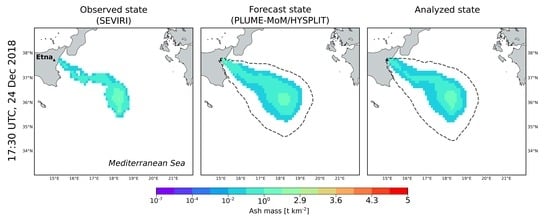
The results of the assimilation procedure are shown from
Figure 5,
Figure 6,
Figure 7 and
Figure 8. At each assimilation cycle, three ash states are presented. From the left to the right, these are: the ash cloud as seen from space (Observations), the prediction done by the model (Forecast state) and the result of the assimilation procedure (Analyzed state). The statistics describing each ash state are the mean value and the standard deviation calculated for the ash columnar content of each pixel. For the forecast and analyzed states, these quantities are computed from the ensemble members by applying Equations (
1) and (
2) (standard deviation is the square root of the covariance). The mean state is displayed in
Figure 5 and
Figure 6, while the standard deviation in
Figure 7 and
Figure 8. For the forecast and the analyzed states, ash load (kg) contained in each pixel was integrated over the particle classes and the atmospheric levels to produce 2D maps. Then, ash load was converted into ash columnar content (t km
) for comparison with the SEVIRI observations. A concentration cut-off of 0.01 t km
was applied to the plot of observations, forecast and analyzed states. Despite the concentration cut-off, 99% of the initial ash loading is still present into the regions plotted in the figures for the measured, forecast and analyzed ash states. It is worth noting that the simulated clouds are bigger than the observed ones. This result is mainly due to the way in which the ensemble was created, which is through perturbations of the wind-field. Changing the way in which the ensemble is generated (e.g., through perturbations of ESPs such as column height or TGSD) or varying the perturbation coefficients (i.e.,
,
,
,
) would affect the size and the shape of the simulated cloud. These effects can be seen in the experiments reported in the
supplementary material (Figures S1–S25).
From
Figure 5 and
Figure 6 it emerges that the analyzed state produced by the DA cycle improves the numerical ash forecasting by taking into account the observations. This is evident starting from the first assimilation cycle (12:30), where the peak in ash column amount of the forecast state was modified considering the observed state. The ensemble members forming the analyzed state at each assimilation cycle were used to reinitialize the dispersal simulation to provide a new forecast.
The ability of the filter in producing a new analyzed state with minimized errors is evident when looking at the standard deviations computed for the observed, forecast and analyzed states (
Figure 7 and
Figure 8).
Evaluation metrics were computed to check the performance of the numerical model in producing the forecast states used in the assimilation procedure. Panels from (a) to (g) of
Figure 9 show the rank histograms computed for the different time slices (i.e., 12:30, 13:30, 14:30, 15:30, 16:30, 17:30 and 18:30), while Panel (h) presents the cumulative histogram obtained by summing histograms from (a) to (g). Each histogram was constructed by considering all the points of the computational domain and by applying a concentration cut-off of 0.01 t km
, to be consistent with the procedure previously applied. This means that ensemble values less than 0.01 t km
were replaced with zero. Rank histograms appear flat, without peaks at the extremes (U-shaped) or at the central bins (Dome-shaped). This means that the ensemble spread is appropriate in reproducing the actual model uncertainty, with the higher bias for times 16:30 and 17:30. This result can be partially due to the fact that in most of the pixels of the domain there is a zero concentration for both the ensemble members and the observation. For this reason, to better analyze the local performance of the data assimilation algorithm, we also computed the Rank Probability Score (
) for each pixel presenting an observation value different from zero.
allows us to check the accuracy of the ensemble prediction locally (i.e., at each observation point), see
Figure 10. The magenta pixels in
Figure 10 indicate the observations falling outside the range of values predicted by the model. About 95% of the observed values are within the predicted values and
range from 0 to 0.4 (0 means perfect prediction).
Overall, the rank histograms and the indicate that our ensembles are reliable in reproducing the true variability of the observations and thus they can be used for the DA procedure.
At each assimilation time, True Positive, False Positive and False Negative areas were computed from the observed and the forecast clouds (
Figure 11). The number of pixels forming each region was used to calculate indices
,
and
by applying Equations (
12)–(
14). As previously stated, high values of
are necessary to ensure reliable assimilation results. We found that the creation of the ensemble members through perturbed versions of a reference wind-field allows us to obtain high values of
. Indeed, excluding the first assimilation cycle (12:30),
computed for the following cycles is close to 100% for all the experiments, see
Table 4.
The performance of the filter has been evaluated through the
computed by applying Equation (
15) for the forecast and the analyzed states and Equation (
16) for the observations.
Figure 12 shows the
evaluated for the 6 experiments. It can be noticed that the
of the forecast and the analyzed states decrease as the assimilation cycles are performed. This trend is shared by all the experiments and indicates that the assimilation progressively reduces the uncertainty of the simulated ash clouds, both forecast and analyzed. Moreover, at each assimilation cycle, the analyzed states have a
lower than the forecast states. This means that the assimilation procedure results in a new state where the uncertainty on ash amount and spatial distribution is minimized with respect to the predicted state.
Results of EXP1, EXP2 and EXP3 (Panels (a), (b) and (c) in
Figure 12) are similar in terms of
, while a variation can be observed for EXP4, EXP5 and EXP6 (Panels (d), (e) and (f) in
Figure 12). This means that similar filter performance is obtained varying the angle used to perturb the wind-field (15
for EXP1, 10
for EXP2 and
for EXP3).
On the contrary, the observation sampling time (1 h for EXP1, EXP2 and EXP3; 30 min for EXP4 and 2 h for EXP5) plays a more incisive role in filter performance. Indeed, short observation sampling times (30 min of EXP4) force the convergence of the analyzed state toward the forecast state. This is because, after each model re-initialization, the advection/diffusion mechanisms acting on the puffs forming the cloud have a limited time window to act before a new assimilation is done. Thus, the forecast state at time t remain similar to the analyzed state at time t and so their .
of the observations are independent from the sampling time interval and, for this case study, are always higher than the
of the forecast states. For this reason, the forecast states have a higher influence on the assimilated states than the observations. From
Figure 12 it can be seen that long observation sampling times (2 h for EXP5) allow the advection/diffusion mechanisms to increase cloud spreading and thus to reduce filter convergence rate. A different trend emerges for EXP6 for which ensemble members have been created both by perturbing the wind-field and by considering the height of the eruptive column unknown (1000, 4000, 8000 and 12,000 m above the vent). The forecast
computed for the first assimilation cycle (12:30) is about 250 t. This value is one order of magnitude higher than that computed for the other experiments (11 t). However, the analyzed state resulting from the first assimilation cycles has a
of 75 t, which is 70% lower than the
of forecast state. This trend is maintained for the following cycles and starting from the 14:30 assimilation cycle the forecast and analyzed
are consistent with what found in the previous experiments. EXP6 shows that DA enables a strong reduction to the uncertainties deriving from the initialization of the numerical model with highly uncertain ESPs. This result is of great value for the number of applications where ESPs are unknown or difficult to estimate in real time. Indeed, while Mt. Etna is extensively monitored from the ground and from space, the majority of worldwide volcanoes are not monitored [
89] and ESPs are difficult to be assessed in real time when eruptions occur. In such cases, we found that the effects of highly uncertain ESPs are limited to the first assimilation cycles only and that the filter allows a significant reduction of the
leading to results which are similar to well-constrained cases (i.e., EXP1, EXP2 and EXP3).
Figure 13 shows the total atmospheric ash mass loading computed for the observed, forecast and analyzed states as the assimilation cycles are performed. Satellite retrievals report about 10 kt of fine ash released during the eruption. It is worth noting that the forecast ash loadings are higher than the analyzed loadings computed at the previous assimilation cycle. This because a continuous ash emission is simulated during the experiments. The trend shared by the 6 experiments is the tendency of the analyzed ash loading to converge to the observed one as the assimilation cycles are performed. This is particularly evident for EXP6, where the forecast ash loading at the first assimilation cycle (12:30) is 253 kt. This high value is due to the creation of the ensemble members through perturbations of volcanic column height, and thus mass flow rate. Thanks to the assimilation, the analyzed ash loading at 12:30 drops to 70 kt. This value further decreases to 31 kt at 13:30 and to 22 kt at 14:30. At the end of the assimilation experiment (18:30), the analyzed ash loading is 12 kt, which is a value in line with the 10 kt retrieved from space. This example highlights that sequential EnKF does not need a precise initialization of the numerical model. It is the filter that calibrates the analyzed state considering the uncertainties on observations and numerical predictions.
8. Conclusions
We presented the implementation of a Data Assimilation procedure inside the VATD model HYSPLIT. The aim was developing a methodology to correct the predictions done by HYSPLIT with satellite observations of ash columnar content. To properly simulate explosive eruptions, HYSPLIT was initialized with the results of the eruptive column model PLUME-MoM. The coupling between the two codes has been completely automated and the two models allow us to simulate the release and atmospheric transport of volcanic ash clouds produced by explosive eruptions. The toolkit used to perform the assimilation is the Parallel Data Assimilation Framework (PDAF). PDAF routines were linked to the numerical model to perform the assimilation cycles in an automated way and at prescribed times (i.e., when observations are available). We used the Local Ensemble Transform Kalman Filter and tested it to track the ash cloud produced by the explosive eruption occurred at Mt. Etna on 24 December 2018. Measurements of ash columnar content done by the sensor SEVIRI were used as observations to be assimilated.
We performed different experiments (6 in total) varying both the type of parameters included in the ensembles, their respective ranges, and the observations sampling time. We showed that even the simple application of an ensemble strategy (without EnKFs) makes model predictions more similar to the observed ash cloud than those resulting from single deterministic simulations. This first result enhances the importance of ensemble-based ash forecasting.
Next, we showed how assimilation of satellite data further improve ash monitoring and forecasting. Indeed, the analyzed ash states are less uncertain with respect to both forecast and observed states and the peak in ash column amount is calibrated in agreement with what observed from space.
The ability of EnKF to reduce state uncertainty when ESPs are highly uncertain is another important feature of this kind of filter. In this way, accurate knowledge of ESPs is not mandatory for model initialization enforcing the use of EnKFs for ash forecasting of not routinely monitored volcanoes. Future research could aim at implementing variational filters for the retrieval of initial eruptive parameters from satellite observations.
Although we developed and applied the assimilation procedure to an historical eruption, Data Assimilation is perfectly suitable for real-time applications to track and forecast the advection/dispersal patterns of any ash cloud. Indeed, estimates of ash columnar content are furnished in real time by a variety of satellite sensors. For this reason, this kind of approach has the potential to greatly improve reliability of volcanic ash forecasting done by VATD models, with implications on aviation hazard avoidance. However, additional research is needed to improve the present approach in the context of aviation safety. First, while VAACs respond to volcanic crises producing 3-D ash concentration charts, the retrievals of volcanic clouds made from satellite measurements are in the form of 2-D maps. Information on cloud height and cloud thickness are needed to convert 2-D satellite maps into 3-D data. To that end, some approaches have been developed [
49], but they rely on assumptions about cloud thickness, which is a parameter very difficult to estimate. Thus, additional research is needed to improve the conversion of 2-D satellite maps into 3-D charts. In this way, it will be possible to assimilate directly the 3-D ash concentration and thus to produce outcomes ready to be used for aviation avoidance. Secondly, a distinction between ash-contaminated and ash-free pixels based on concentration statistics and not on a purely binary approach would help to develop a more robust method for aviation risk assessment.
Finally, our approach could be effective also for monitoring and forecasting volcanic SO
clouds. Indeed, as for ash clouds, many satellite sensors can detect and measure volcanic SO
. Beyond SEVIRI, recent example instruments are the sensors TROPOMI [
90] and EPIC [
91]. In particular, TROPOMI enables the detection of SO
produced by passive degassing activity and low intensity eruptions. Since SO
is extremely dangerous for human health, the possibility to accurately forecast the dispersion patterns of such gas is of great value for volcanic risk mitigation.
Overall, we highlight that Data Assimilation aimed at monitoring and forecasting volcanic emissions (both ash and gases) can represent a real breakthrough for improving our assessment of volcanic hazards.

 ,
, 


