A Hybrid Deep Learning Model to Forecast Particulate Matter Concentration Levels in Seoul, South Korea

Abstract

Both long- and short-term exposure to high concentrations of airborne particulate matter (PM) severely affect human health. Many countries now regulate PM concentrations. Early-warning systems based on PM concentration levels are urgently required to allow countermeasures to reduce harm and loss. Previous studies sought to establish accurate, efficient predictive models. Many machine-learning methods are used for air pollution forecasting. The long short-term memory and gated recurrent unit methods, typical deep-learning methods, reliably predict PM levels with some limitations. In this paper, the authors proposed novel hybrid models to combine the strength of two types of deep learning methods. Moreover, the authors compare hybrid deep-learning methods (convolutional neural network (CNN)—long short-term memory (LSTM) and CNN—gated recurrent unit (GRU)) with several stand-alone methods (LSTM, GRU) in terms of predicting PM concentrations in 39 stations in Seoul. Hourly air pollution data and meteorological data from January 2015 to December 2018 was used for these training models. The results of the experiment confirmed that the proposed prediction model could predict the PM concentrations for the next 7 days. Hybrid models outperformed single models in five areas selected randomly with the lowest root mean square error (RMSE) and mean absolute error (MAE) values for both PM₁₀ and PM_2.5. The error rate for PM₁₀ prediction in Gangnam with RMSE is 1.688, and MAE is 1.161. For hybrid models, the CNN–GRU better-predicted PM₁₀ for all stations selected, while the CNN–LSTM model performed better on predicting PM_2.5.

1. Introduction

Recently, particulate matter (PM) levels have become a global problem. PM₁₀ and PM_2.5 are fine particles with aerodynamic diameters smaller than 10 and 2.5 µm, respectively [1]. Many epidemiological studies have shown that PM, especially at high concentrations, is very toxic to humans [2]. PM₁₀ and PM_2.5 levels are strongly correlated with human health—the non-accidental mortality increased by 0.36% and 0.40% for a 10 µg/m³ increase of PM₁₀ and PM_2.5. Short-term exposure to high PM₁₀ and PM_2.5 concentrations increases cause-specific mortality [3], and long-term exposure may cause temporary cardiopulmonary effects, respiratory diseases, and even lung cancer [4,5,6]. Especially, the World Health Organization (WHO) classified PM_2.5 as a first-degree carcinogen and announced that monitoring of PM₁₀ and PM_2.5 needs to be improved in many countries to assess population exposure [7]. As high PM concentrations stunt growth and increase mortality, many countries carefully monitor daily airborne PM concentrations [7]. Most countries have national air quality standards for pollutants considered harmful to public health and the environment. The WHO Air Quality Guidelines (AQG) and European Union (EU) set pollutant concentrations’ thresholds that shall not be exceeded in a given period [8]. In WHO AOG, hourly concentration thresholds of PM₁₀ or PM_2.5 are 50 or 10µg/m³, respectively. In South Korea, average 24 h mean PM₁₀ or PM_2.5 concentrations of >100 or >35 µg/m³ respectively, are recognized as high-concentration [9]. In Korea, the government takes emergency actions to immediately reduce the emissions and protect the people against harmful particle pollution when high concentrations of PM2.5 are predicted to occur or continue. The actions include adjusting operation levels of coal-fired power plants, construction sites, and emission facilities, and driving bans for cars with high emissions.

The real-time PM concentration data are essential when seeking to control air pollution and reduce the effects of PM on health. A real-time warning system for the high concentration of PM is necessary. These warning systems based on reliable predicting models contribute to reduce the PM impact on public health and reduce the casualties and financial losses.

Many predictive methods have been developed, and are either deterministic or statistical. Deterministic methods use chemical and physical data to model pollution processes [8], whereas statistical methods predict PM concentrations using sophisticated theoretical approaches. Some of these methods reliably predict air pollution episodes [10,11,12]. However, traditional statistical models (such as autoregression) do not recognize non-linear patterns, rendering air pollution forecasting over time difficult. Given the rapid developments in hardware and big data management, machine-learning methods (particularly deep learning) have become popular. Many of these methods are used for time-series predictions and have proven reliable. An artificial neural network (ANN) as a classical form of machine learning handles non-linear mapping problems rather well, as there is no need to pre-specify a particular model [13]. ANN models deliver better PM forecasts than do other basic machine-learning methods [14,15].

The shortcoming of ANN-based models is lack of memory cell make it hard to find the connections of inputs given the long time series. Typical recurrent neural network (RNN) models, which feature deep-learning employing a unique recurrent structure, have found applications in speech recognition [16] and machine translation [17]. Natural language processing requires time sequences, and RNNs handle time series well. Such models yield time-series predictions [18,19] and are well-suited for supervised learning using sequential data patterns. In terms of sequential time-series predictions, the recurrent units remember earlier data, processing not only new data but also previous outputs to generate up-to-date predictions. All RNN layers feature unique recurrent units that address temporal order and sequence-dependencies [20]. RNNs can process arbitrary sequences [21].

However, RNNs find it difficult to handle long-term dependence when processing inputs and sequences. Also, plain-vanilla RNNs can exhibit a vanishing gradient problem such that the networks (especially deep neural networks) only learn and no longer predict. The long short-term memory (LSTM) and gated recurrent unit (GRU) cells are optimal for time-series forecasting and do not have the problems that RNN faces. Hochreiter and Schmidhuber developed the gated memory unit termed LSTM [22]. LSTM memory blocks feature one or more recurrent memory cells, and they input, output, and forget units that read, write, and reset information. Compared to RNNs, LSTM neural networks can handle long-term data series predicting future time series. Moreover, the gradient problem is eliminated. A GRU [17], a type of recurrent cell, is similar to but simpler than an LSTM. Both cell types may be useful for prediction. Three popular RNN cells were compared in Reference [23] in the context of short-term load forecasting, and LSTM and GRU cells afforded similar performances and were better than the plain RNN. The performance of convolutional neural networks (CNNs) is comparable to that of RNNs [24]. Indeed, compared to pure RNNs, CNNs may be more efficient—vanishing or exploding gradients are absent [25]. CNNs may perform better when trained using multiple, similar time-series inputs [26]. These deep learning models have been successfully applied to predict problems.

However, most studies focus on single models which have their limitations. RNN-based models are capable of long-term prediction but with much longer training time and computation resources. In this paper, the authors focus on these methods to explore the predictive utility of stand-alone and hybrid models in forecasting PM concentrations in Seoul, South Korea. The proposed hybrid methods have less training time and higher predicting accuracy compared to single models.

Section 2 of the paper prepares relative material for model training. Section 3 explains the proposed models and the training workflows. Section 4 deals with hyperparameter tuning and gives detailed experiments. Section 5 compares the predictions afforded and model performances, and Section 6 contains the conclusions and future research directions.

2. Materials

2.1 Observation Stations

The Korean Ministry of Environment installs and operates an air pollution monitoring station nationwide to monitor the nation’s air pollution status, trends in change, and whether air quality standards are achieved. In this paper, 39 observation stations in Seoul were selected for the study of PM concentration level forecast. Figure 1 shows the location of the air pollution monitoring stations, with two types of monitoring stations occupied in Figure 1. 25 city air monitoring stations distributed in 25 districts in the whole of Seoul city are marked in red, and the green markers in Figure 1 represent the location of each roadside monitoring station.

Table 1. Selected monitoring stations in Seoul.

Type	Station	Site Code	Location	Latitude	Longitude
Urban	Gangnam-gu	111261	426, Hakdong-ro	N 37.5181	E 127.0472
Urban	Gwangjin-gu	111141	571, Gwangnaru-ro	N 37.5441	E 127.0930
Urban	Dobong-gu	111171	34, Sirubong-ro 2-gil	N 37.6627	E 127.0269
Urban	Gangdong-gu	111274	59, Gucheonmyeon-ro 42-gil	N 37.5431	E 127.1255
Urban	Gangseo-gu	111212	71, Gangseo-ro 45da-gil	N 37.5446	E 126.8350
Roadside	Seoul Station	111122	405, Hangang-daero	N 37.5544	E 126.9717
Roadside	Jongno	111125	169, Jong-ro, Jongno-gu	N 37.5708	E 126.9965
Roadside	Gonghangro	111213	727–1091, Magok-dong	N 37.5678	E 126.8348
Roadside	Cheonho-daero	111275	1151, Cheonho-daero	N 37.5341	E 127.1510
Roadside	Yangjaedong	111264	201, Gangnam-daero	N 37.4820	E 127.0362

shows the detailed location information of 10 of the 39 monitoring stations. All these stations collect air pollution data every hour of the day, all data are provided on the AirKorea website (http://www.airkorea.or.kr) by the Korean Environmental Corporation. The collected air pollution data include PM₁₀, PM_2.5, O₃, CO, SO₂, and NO₂. The authors used PM₁₀ and PM_2.5 data collected from 1 January 2015 to 31 December 2018 for this study because PM_2.5 data has been released since 2015. The two types of monitoring stations were treated in the same way, and only PM₁₀ and PM_2.5 hourly concentrations were used for research in this paper.

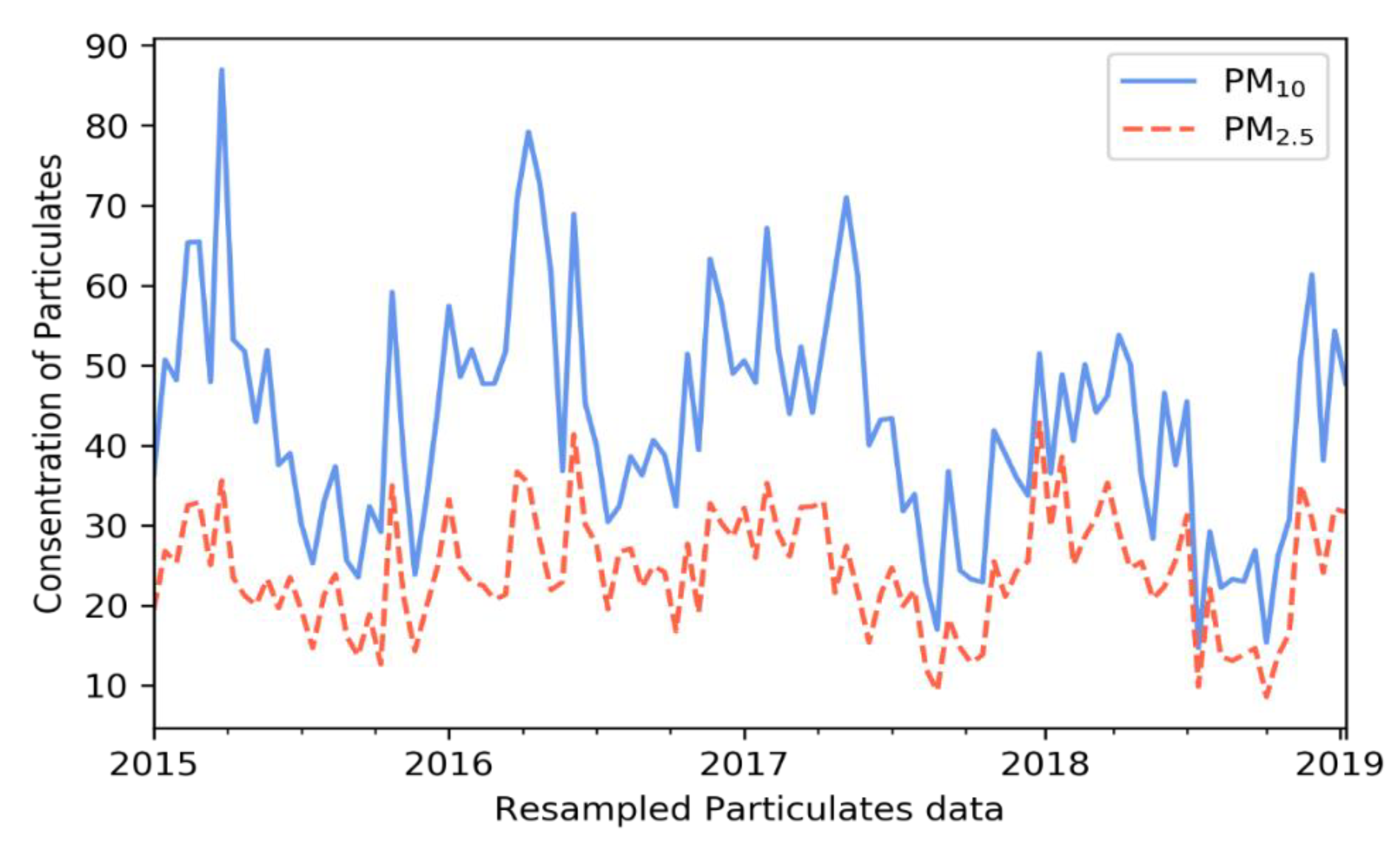
2.2 Data Description

The input variables that are significant in terms of predictive reliability were used. Prior air pollutant concentrations are essential. As local meteorological data strongly correlated with pollutant concentrations, the authors used some meteorological data for training. The Seoul meteorological data collected from 1 January 2015 to 31 December 2018 used in the study was provided by the Korea Meteorological Administration website (http://data.kma.go.kr). Many factors affect local PM accumulation or dissipation, including temperature, wind, and rain. Temperature is important when predicting PM concentrations [27], as high temperatures are associated with stable high-pressure atmospheric conditions, favoring PM accumulation. Low relative humidity and low temperature correlated with locally high PM_2.5 concentrations [28]. Wind transports PM horizontally [29], and low wind speeds tend to be associated with high PM concentrations because wind directly affects PM dispersion [30]. Rain eliminates PM and dust in the air. Thus, PM concentrations are usually lower in summer seasons because of frequent and heavy rain, and higher in the winter season, which has less rainy days.

Meteorological datasets contain several features. Wind direction ranges from 0 to 360°, and wind speed followed the Beaufort wind scale from 0 to 12 to represent how fast the wind is blowing. In Reference [31], southern and eastern wind directions and speeds were derived using a periodic cosine function:

$$\mathrm{Wind}\_\mathrm{x}=w \cos \mathsf{\alpha }$$

(1)

$$\mathrm{Wind}\_\mathrm{y}=-w \sin \mathsf{\alpha }$$

(2)

where α is the wind direction, and w is the wind speed.

To explore the correlations between inputs, the authors used Pearson correlations between 9 training inputs of the Gangnam dataset in

Table 2. Correlations between input factors.

	PM10	PM2.5	Temperature	Sky Condition	Rain	Humidity	Rain Condition	Wind_x	Wind_y
PM10	1.0000	0.7763	−0.1637	−0.0537	−0.0509	−0.0809	−0.0355	−0.0031	0.0049
PM2.5	0.7763	1.0000	−0.1242	−0.0110	−0.0394	0.0316	−0.0197	0.0075	−0.0014
Temperature	−0.1637	−0.1242	1.0000	0.2685	0.0510	0.1477	−0.0519	0.0068	−0.0113
Sky condition	−0.0537	−0.0110	0.2685	1.0000	0.1234	0.3265	0.2314	−0.0050	−0.0040
Rain	−0.0509	−0.0394	0.0510	0.1234	1.0000	0.1756	0.2625	0.0068	0.0009
Humidity	−0.0809	0.0316	0.1477	0.3265	0.1756	1.0000	0.2614	0.0019	−0.0061
Rain condition	−0.0355	−0.0197	−0.0519	0.2314	0.2625	0.2614	1.0000	0.0040	−0.0065
Wind_x	−0.0031	0.0075	0.0068	−0.0050	0.0068	0.0019	0.0040	1.0000	−0.0028
Wind_y	0.0049	−0.001	−0.0113	−0.0040	0.0009	−0.0061	−0.0065	−0.0028	1.0000

* bold values are the correlation of same factor as 1.0000.

. For PM₁₀ and PM_2.5 concentrations, correlations ranged from −1 to 1, with a higher absolute number indicating a higher correlation. A positive number indicates a positive correlation between two factors, and a negative number indicates negative correlations. The greater the number is, the higher the correlation is. PM₁₀ and PM_2.5 levels were highly correlated. Using the original data, the correlation between the two columns, as seen in Table 2, was 0.7763. When the authors resampled the original data into weekly mean data, the correlation between the mean weekly values was 0.8017. Thus, an element of hidden correlation was present, which deep-learning models can capture.

Figure 2 shows the trends of PM concentrations. The two data columns were resampled to yield two single-point weekly values, making it easier to capture changes. In this case, the levels of the two PM types exhibited similar trends.

Temperature, wind speed, and rain were negatively correlated with air pollutant concentrations, facilitating NN learning. Thus, forecast PM₁₀ levels were affected by PM_2.5 and meteorological data.

Air pollution data and meteorological data were combined into one dataset for each station in Seoul. Each dataset contains nine input feathers as hourly PM₁₀ concentration, PM_2.5 concentration, the temperature at a local station, sky condition at a local station, rainfall, relative humidity, rain condition, wind_x, and wind_y. These nine features were used as inputs for training models in this paper.

All training models featured nine input variables, including PM_2.5 and PM₁₀ concentrations. Each dataset was generated by a monitoring station and contained 4 years of data, from 2015 to 2018. Each dataset was divided into training (70%), validation (27%), and test datasets (3%). The 4-year data from 2015 to 2018 was divided into 1018 days for training, 392 days for validation, and 43 days for testing. The trained models were tuned using the validation datasets, and the predictions were compared with reality. Deep-learning models may become confused if values are missing or abnormal, compromising the outputs. Thus, historical data may be lost. When this arose, the researchers input a value of 0. Also, some data may be incorrectly recorded (machine or human error). For example, on several days, PM₁₀ concentrations exceeded 1000 µg/m³ (several cases with extremely high concentration but show no connection with the next or previous data in the dataset) or were less than 0 µg/m³ (as common sense), replaced by 0. The input ranges are listed in

Table 3. Training data and model parameters.

Variable	Measurement Unit	Range
PM2.5	µg/m3	0~180
PM10	µg/m3	0~400
Temperature	°C	−25~45
Rain	mm	>0
Wind_x	Float	−12~12
Wind_y	Float	−12~12
Humidity	%	0~100
Rain	Integer	0, 1, 2, 3
Sky	Integer	1, 2, 3, 4

. PM_2.5 and PM₁₀ concentrations were within the normal range, and the temperature ranged from −25 to 45 °C. Wind_x (southern wind), as a float number calculated by wind speed, and wind direction ranged from −12 to 12, and wind_y (eastern wind), as a float number, ranged from −12 to 12, in South Korea. In terms of rain status, 0 indicates no precipitation, 1 is rain, 2 indicates sleet, and 3 is snow. In terms of the sky, 1–4 indicate sunny, partly cloudy, cloudy, and dark skies, respectively.

The models feature various cell activation functions. The sigmoid and tanh functions may become saturated, rendering the outputs near constant. Thus, the input data require normalization before forward feeding into the training model, as the outputs must not be saturated [32]. The authors used the MinMaxScaler to normalize training data, so all features were scaled in the range 0 to 1.

3. Methodology

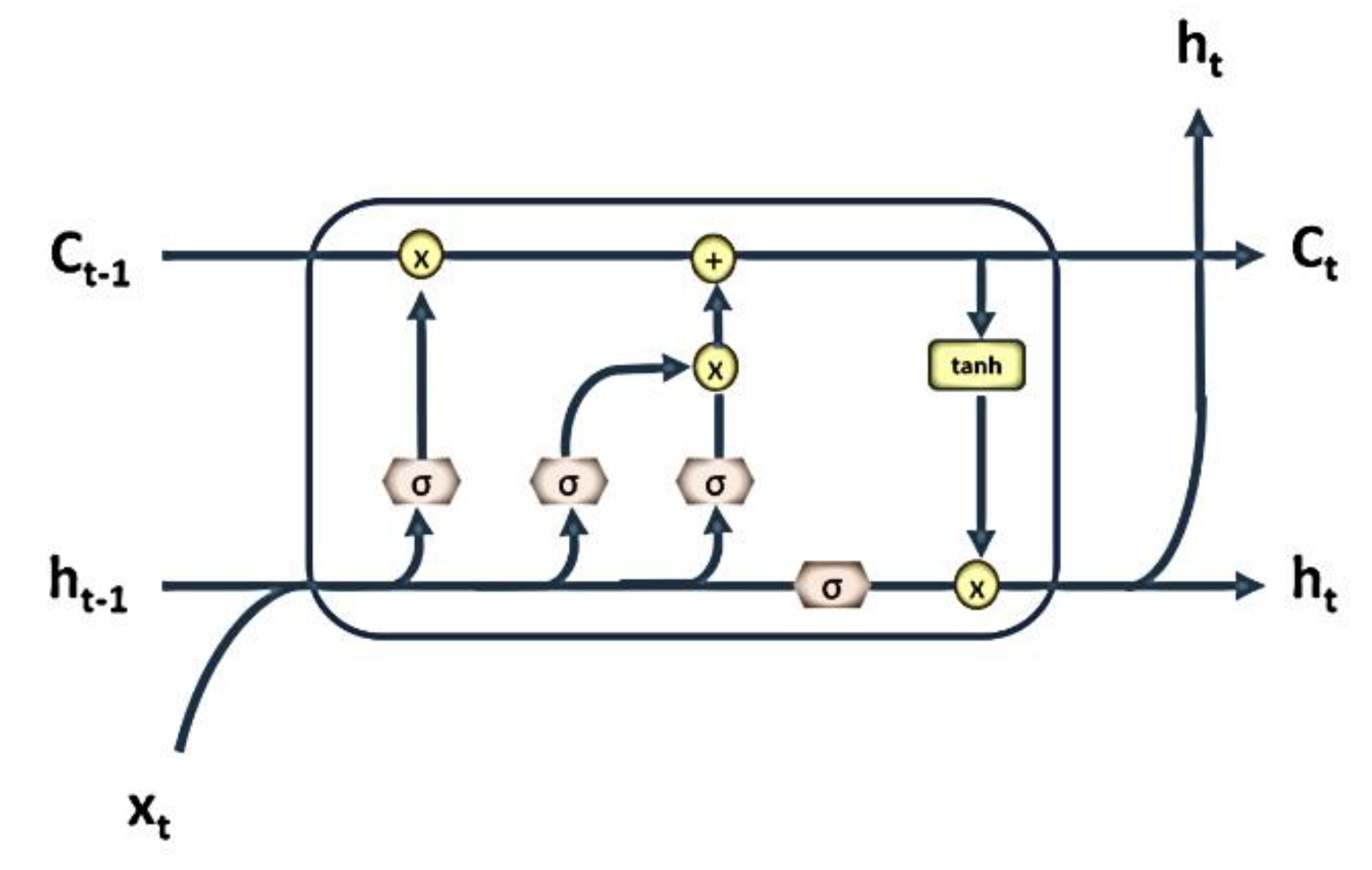
3.1 The Long Short-Term Recurrent Unit

The structure of a single recurrent LSTM unit is shown below (Figure 3).

$$f_t=\sigma (W_f·[h_{t-1},x_t]+b_f)$$

(3)

$$i_t=\sigma (W_i·[h_{t-1},x_t]+b_i)$$

(4)

$${\stackrel{\sim }{C}}_t=tanh(W_c·[h_{t-1},x_t]+b_c)$$

(5)

$$C_t=f_t\ast C_{t-1}+i_t\ast {\stackrel{\sim }{C}}_t$$

(6)

$$h_t=\sigma (W_o·[h_{t-1},x_t]+b_o)\ast tanh(C_t)$$

(7)

These equations show that LSTM cells in recurrent layers process data forward. i refers to the operation of input, o refers to output operation, and f refers to the operation of the forgetting gate. t is the current time, and t – 1 is a previous time. h stands for hidden state and C refers to cell state, W and b are the weight and bias vector, σ is the sigmoid activation function, and tanh is the hyperbolic tangent activation function. Formula (3) is a function of the forgetting gate, which decides how much state data to preserve. Equation (4) shows how the input gate determines the values to be updated, and Equation (5) defines the candidate value ${\stackrel{\sim }{\mathrm{C}}}_{\mathrm{t}}$ to be added to the cell state. Equation (6) manages cell state update. The old state is multiplied by f_t, and the values are summed and added to the results of the multiplication of the input gate state and the candidate. This determines how much information is updated to the new cell state C_t. Equation (7) determines what proportion of the cell state will serve as the output, and this is multiplied by the cell state filtered by the hyperbolic tangent function to generate the final output.

3.2. The Gated Recurrent Unit

The structure of a GRU is shown in Figure 4, and the formulae below indicate how the recurrent unit processes sequence data forward.

$$z_t=\sigma \left(W_z·\left[h_{t-1},x_t\right]+b_z\right)$$

(8)

$$r_t=\sigma \left(W_r·\left[h_{t-1},x_t\right]+b_r\right)$$

(9)

$${\tilde{h}}_t=tanh\left(W·\left[r_t\ast h_{t-1},x_t\right]+b_h\right)$$

(10)

$$h_t=z_t\ast {\tilde{h}}_t+\left(1-z_t\right)\ast h_{t-1}$$

(11)

where x denotes the input vector, h is the output vector, z is the update gate vector, r is the reset gate vector, w and b are the weight and bias respectively, and t is the time. As is true of the LSTM unit, the GRU features gates processing data forward to the unit. The principal differences between the two methods lie in their gates and weights. A GRU has two gates, the update gate and the reset gate. The update gate performs functions similar to the forget and input gates of the LSTM, and the reset gate decides how much past information to forget. Equation (8) shows how the update gate controls new information and information generated by previous activations. Equation (9) shows which reset gate activity is included in candidate activation. Equations (10) and (11) combine the candidate state with previous output and filter the data to obtain the output of the current state.

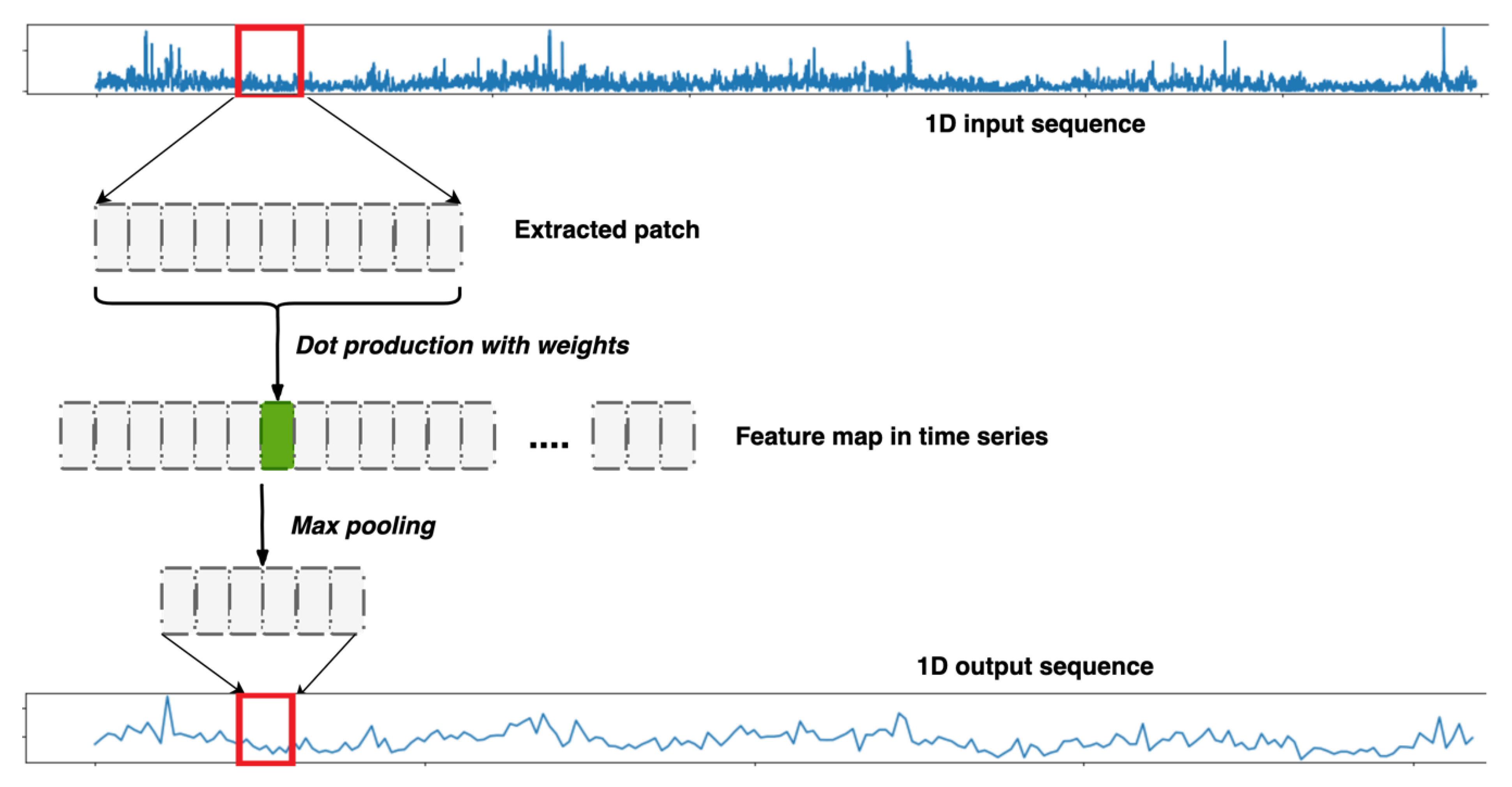
3.3. Convolutional Layers

A one-dimensional convolutional neural network (1DConvNet) can handle local patterns in time-series sequences. In terms of time-series forecasting, the time sequence is treated as a spatial dimension (similar to two-dimensional height or width), which is optimal in our present context. Identical input transformations were performed on all extracted patches, so a specific pattern learned at the current position can be recognized in a different position.

Figure 5 shows the processing of a single-feature input over time by the 1DConvNet. The window size used for sequence processing can be predefined, and fragments learned in sequence. These learned subsequences can then be identified wherever they occur in the overall sequence. ‘Max pooling’ reduces the lengths of input sequences, as CNN learns their critical parameters. In this paper, the researchers applied the 1DConvNet to our proposed models, as introduced in Section 3.

3.4. Hybrid Models

In this paper, hybrid CNN–LSTM and CNN–GRU models are used to predict local PM₁₀ and PM_2.5 concentrations. The authors assume that with the one-dimensional convolutional layer, it is possible to recognize local patterns based on the feature of 1DConvNet, and recurrent layers are designed to capture useful patterns to forecast the future. By combining convolutional layers and RNN layers, the hybrid models expected to capture hidden patterns and deliver reliable predictions.

The structure of the CNN–LSTM model is illustrated in Figure 6. The model features four layers with different neuron types and numbers. The data were fed into a one-dimensional convolutional layer, an LSTM layer stack on top of that layer, a fully connected dense layer stack on the LSTM layer, and the top layer is the output layer with two neurons.

To allow among-model comparisons, the CNN–GRU model has a similar structure. The model processed nine input variables. The first layer is a one-dimensional convolutional layer with 64 neurons, the second layer is a recurrent layer with 32 GRUs, and the third and final layers are dense. The principal difference between the two models is the inner structure of the recurrent layer.

3.5. General Workflow

In this paper, the authors explored how well four models predicted air pollutant concentrations in several regions of Seoul. The training workflow is illustrated in Figure 7:

The steps are:

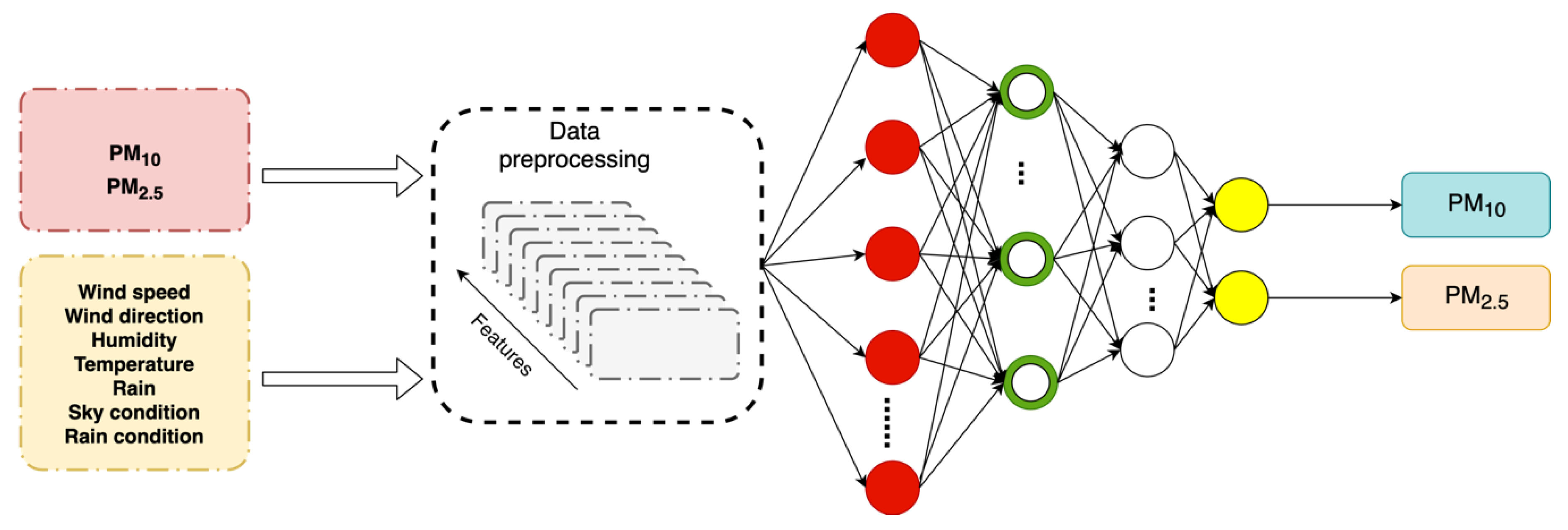
• Data choice. Good-quality training data are essential. For each specific model, the data type and attributes must be chosen carefully. The authors used pollution data and meteorological data to train models, combining several training factors (hourly particulates concentrations and meteorological data) into one dataset, aligning the different types of data at the same time points.
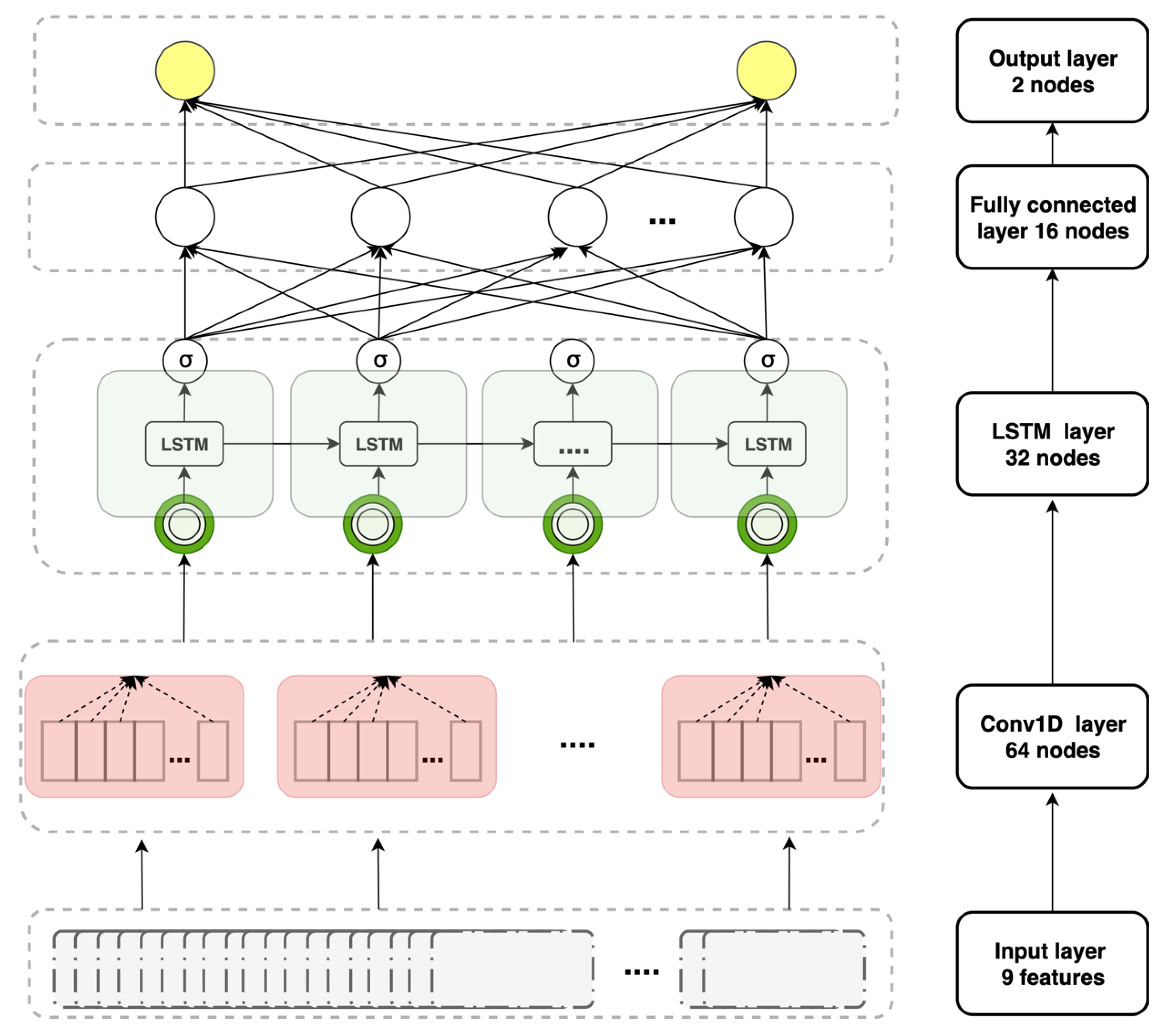
• Data preprocessing. The researchers used various data preprocessed via different methods to generate inputs to the NNs. The specific preprocessing methods used met the requirements of the training models. For example, the first layer of (the input to) the LSTM model was an LSTM layer.
• Model training. The models use input data to learn hidden features. The training model structures differ. For the LSTM model, the green layer with recurrent units is an LSTM layer, the white layer is fully connected, and the last layer is the output layer. Training requires tuning of the various hyperparameters that affect training and model performance.
• Hyperparameter tuning. During model training, many hyperparameters must be defined or modified to optimize predictions. Model hyperparameters differ, and all models were optimized before comparison.
• Output generation. After training, the best model was identified, and the success of training was evaluated by inputting test data. Both the PM₁₀ and PM_2.5 concentrations served as outputs. Thus, the output layers featured two neurons.
• Model comparison. All models were trained to generate predictions. The authors used all models to predict air pollution concentrations in the same area and then identified the most suitable model.

4. Experiments and Results

4.1. Evaluation Methods

In this paper, root mean square errors (RMSEs) and mean absolute errors (MAEs) were calculated when comparing predictions with actual values. Smaller values indicate better performances. The RMSE imparts relatively high weights to large errors. The formulae are:

$$\mathrm{RMSE}=\sqrt{\frac{1}{n}{\displaystyle \sum _{i=1}^n{({\mathrm{y}}_{\mathrm{i}}-{\hat{\mathrm{y}}}_{\mathrm{i}})}^2}}$$

(12)

$$\mathrm{MAE}=\frac{1}{n}{\displaystyle \sum _{i=1}^n|{\mathrm{y}}_{\mathrm{i}}-{\hat{\mathrm{y}}}_{\mathrm{i}}|}$$

(13)

where n is the number of sampled data in the test set, y_i is a sample i of the predicted data, and ${\hat{\mathrm{y}}}_{\mathrm{i}}$ is the real i value.

4.2. Model Tuning

The model structure must be defined when comparing performance. Before training, many NN factors affect performance, and when one-factor changes, the resultant prediction changes. These factors, termed hyperparameters, must be carefully chosen. A model is optimized via hyperparameter tuning. General hyperparameters include the number of layers in a neural network, the node numbers in each layer, the learning rate, and layer activation and loss functions. Initially, the authors optimized the GRU model and ensured that the hyperparameters of the other models were similar to the GRU values. For example, a simple GRU model with four layers and 32 neurons set for recurrent layers and the columns contain PM₁₀ and PM_2.5 data were shifted in given length, the shifted length called ‘lookback’. We tuning the length of ‘lookback’ as it can dramatically affect predictions. Thus, the researchers change lookback while holding the other hyperparameters fixed, as shown in

Table 4. The effects of lookback length.

Shift Time (h)	PM10 (RMSE)	PM2.5 (RMSE)
1	11.798	7.719
6	26.230	12.497
12	26.096	13.266
24	11.789	6.997
48	16.598	9.642
72	21.127	10.010

* RMSE: root mean square error; Bold values are best predicted case for PM₁₀ and PM_2.5.

.

When lookback increased, the predictions either failed to improve or deteriorated monotonously. A long lookback (72 h) compromised performance, as irrelevant data were included. Too-short lookback (<12 h) data were unstable, perhaps because previous data were lacking, but nonetheless, the researchers used these data. In Table 4, both PM₁₀ and PM_2.5 had best performance with the lowest error when lookback was set as 24 h. Therefore, the researchers decided to use 24 h as the lookback for these models.

To find the suitable number of layers and number of neurons in each layer, the researchers tuning one single model at first, then applied the layer structure of tuned model to other models.

Table 5. The effects of neuron numbers.

Number of Layers	Results (RMSEs)	Number of Neurons in Each Layer
		16	32	64	128	256	512
3	PM10 PM2.5	14.394 10.323	14.313 10.528	14.818 10.696	14.493 10.667	15.408 10.659	15.046 10.709
4	PM10 PM2.5	13.537 9.667	14.337 9.914	12.516 9.678	12.908 9.911	13.012 10.334	14.589 10.463
5	PM10 PM2.5	14.124 9.850	12.902 9.304	13.609 9.963	13.956 10.207	13.404 9.884	14.416 9.980

* Italics marked value represent the best cases for PM10 and PM2.5 when comparing layer number while number of units in each layer is same (view in each column). Bold values are best cases for PM10 and PM2.5 when comparing number of units in each layer while layer number selected as 4 or 5 (view in each row).

shows the results predicted upon tuning the GRU model. When tuning layer and neuron numbers, the other hyperparameters are fixed.

To explore the number of layers for this model in Table 5, assuming each column represents that the number of units is the same in all layers, values with italic style font in each column represent the best case. By comparing the prediction results of different layers with the same unit numbers, the four-layer structure has seven best cases for PM₁₀ and PM_2.5 in general. The five-layer structure has five best cases, and the three-layer structure did not perform ideally. Thus, the researchers chose four-layer and five-layer structures for further experiments with the GRU model.

As the number of layers chosen was four or five, further experiments keep the number of layers fixed and increase the number of neurons in each layer from 16 to 512, as shown in Table 5. Values with bold font represent the best case in each row. For the four-layer structure, 64 units have the best performance for PM₁₀, and 16 are considered as the best cases for PM_2.5. For the five-layer structure, 32 had the best neuron numbers for both PM₁₀ and PM_2.5 prediction. When the layer number was held constant, and with the neuron number increased, the model did not improve while more training time and more resource consumption occurred. Thus, the maximum neuron number in each layer was defined as 64. The researchers chose 64, 32, and 16 as the number of neurons for further experiments.

Other hyperparameters (number of epochs, learning rate, layer drop rate, activation and loss functions, and weight initializing scheme) were similarly tuned. The models featured CNN, RNN, and fully connected layers. The authors tuned the single GRU and LSTM models and then built hybrid models with the same layer and unit numbers. All models were trained using the same hardware, software, and dataset, and all models ran in TensorFlow on Nvidia Quadro 4-core P4000 GPU (graphics processing unit) and an Intel Xeon 3.3 GHz CPU (central processing unit). The layers of the various models had different attributes, the details of which are listed in

Table 6. Layer attributions of the predictive models.

Model	Attribution	First Layer	Second Layer	Third Layer	Fourth Layer
GRU	Layer type	GRU	GRU	FC	FC
	Number of nodes	64	32	16	2
	Number of parameters	14,208	9312	528	34
	Activation function	tanh	ReLU	linear	linear
	Remarks	Recurrent activation: hard_sigmoid. Return sequences: True.
LSTM	Layer type	LSTM	LSTM	FC	FC
	Number of nodes	64	32	16	2
	Number of parameters	18,944	12,416	528	34
	Activation function	tanh	ReLU	linear	linear
	Remarks	Recurrent activation: hard_sigmoid. Return sequences: True.
CNN–GRU	Layer type	1DConvNet	GRU	FC	FC
	Number of nodes	64	32	16	2
	Number of parameters	13,888	9312	528	34
	Activation function	ReLU	ReLU	linear	linear
	Remarks	Kernel size: 24. Padding: same.
CNN–LSTM	Layer type	1DConvNet	LSTM	FC	FC
	Number of nodes	64	32	16	2
	Number of parameters	13,888	12,416	528	34
	Activation function	ReLU	ReLU	linear	linear
	Remarks	Kernel size: 24. Padding: same.

* FC: fully connected layer; tanh: hyperbolic tangent; ReLU: rectified linear unit.

. LSTM models featured RNN layers with internal LSTM units. The GRU model was similar to the LSTM model, but the recurrent units differed. The hybrid models featured one convolutional and several recurrent layers.

The GRU model featured four layers, the first and second of which were recurrent, with GRU inner units and the neuron numbers listed above. The third layer was fully connected, and the last (output) layer with two neurons. The structure and (certain) attributes of the LSTM model were similar to those of the GRU model. The principal difference lay in the inner structure of the recurrent layers. The LSTM model employed LSTM units. In the CNN–GRU model, the first layer was one-dimensional convolutional, and the second was recurrent with GRUs. The last two layers were fully connected. The principal difference between the hybrid models was that the second layer of the CNN–LSTM model was recurrent with LSTM rather than with GRUs. For all training models, the authors principally used the MSE function to optimize parameters. The Adam optimization algorithm was also employed with the learning rate set to 0.01. The early stopping method was used to pause training when validation loss was not updated after three epochs.

5. Results

The four models were used to forecast up to 15 days of PM concentrations in Seoul. All models were trained using the same datasets. As forecast length increased, accuracy decreased.

Table 7. Fifteen-day predicted results at one station (Eunpyeong-gu).

Prediction Length (Days)	PM10 (RMSE)	PM10 (MAE)	PM2.5 (RMSE)	PM2.5 (MAE)
1	6.547	5.210	4.707	3.889
3	11.450	7.089	5.074	4.046
7	12.010	7.212	5.546	4.096
15	16.096	9.314	7.260	4.633

* RMSE: root square error; MAE: mean absolute error.

shows the predictions of the GRU model for one station. The 15-day predictions remained reliable, and the safest forecasts are up to 7 days in this paper.

Table 8. Seven-day predictions of PM₁₀ levels in five areas.

Area	Evaluation	GRU	LSTM	CNN–GRU	CNN–LSTM
Gangnam-gu	RMSE MAE	12.995 7.981	11.091 6.901	1.688 1.161	2.696 1.959
Songpa-gu	RMSE MAE	15.652 10.124	11.322 7.454	1.620 1.264	2.996 2.259
Seocho-gu	RMSE MAE	14.010 9.648	8.293 6.002	1.246 0.942	2.507 2.073
Gangseo-gu	RMSE MAE	8.976 6.143	7.727 4.919	1.087 0.814	2.162 1.681
Geumcheon-gu	RMSE MAE	9.462 6.777	7.616 5.280	1.096 0.776	1.926 1.495

and

Table 9. Seven-day predictions of PM_2.5 levels in five areas.

Area	Evaluation	GRU	LSTM	CNN–GRU	CNN–LSTM
Gangnam-gu	RMSE MAE	6.987 4.676	6.918 4.603	1.558 1.444	0.867 0.488
Songpa-gu	RMSE MAE	6.816 4.636	6.097 4.241	1.547 1.464	0.788 0.509
Seocho-gu	RMSE MAE	6.058 4.137	5.461 3.413	1.643 1.587	0.608 0.417
Gangseo-gu	RMSE MAE	4.980 3.523	5.387 3.772	1.623 1.518	0.820 0.548
Geumcheon-gu	RMSE MAE	4.813 3.617	4.872 3.702	1.445 1.380	0.872 0.633

* Bold marked values are two best case for each predicting model in each column.

list the 7-day PM₁₀ and PM_2.5 predictions for five Seoul stations derived using the four models. The five stations were Gangnam, Songpa, Seocho, Gangseo, and Geumcheon. All models were trained using the Gangnam dataset—to explore model versatility, 4 of the remaining 38 areas were randomly selected, and 7-day PM concentrations were predicted. Table 8 shows the PM₁₀ predictions. Of the single models, the LSTM performed better than the GRU model in all five stations. The hybrid models were better than a single model for all five stations in this paper. The CNN–GRU model outperformed all other models with all stations for PM₁₀ prediction in this paper. The CNN-GRU model better-predicted PM₁₀ in Gangseo and Geumcheon stations. Other models had better performance in these two stations compared with other stations.

Table 9 shows the PM_2.5 predictive data. The single models performed similarly in five stations. The GRU model better predicted the Gangseo and Geumcheon realities, and the LSTM model was better for Gangnam, Songpa, and Seocho compared to the GRU model. Two single models performed better on Gangseo and Geumcheon stations. The hybrid models outperformed the single models for all stations in this paper, with the CNN–LSTM model being the best of the hybrid models. The CNN–LSTM model generally predicted better than the CNN–GRU model for PM_2.5 predictions. The CNN–GRU model predicted better in the Songpa and Geumcheon stations compared to other stations, while the CNN–LSTM model performed better in the Songpa and Seocho stations in this paper.

Figure 8, Figure 9, Figure 10 and Figure 11 below illustrate the 5-day Gangnam-gu predictions of all models. Each figure compares the PM₁₀ predictions (up), and PM_2.5 predictions (down) yielded by a specific model. The solid blue lines are the real data, and the dashed orange lines show the predicted concentrations. The y-axis is the PM₁₀ or PM_2.5 concentration, and the x-axis shows time in hours. The GRU model generally well-predicted PM trends. In terms of PM₁₀ predictions, the GRU model failed to predict the highest and lowest concentrations over the 5 days. This is of great concern in the sense that such errors compromise early warning. In terms of PM_2.5 predictions, the GRU model predicted high-level pollution episodes, but not periods of low PM.

Compared to the GRU model, the LSTM model better predicted PM₁₀ levels. As shown below, the LSTM predictions were reliable and tracked changing PM concentrations well. The LSTM model well-predicted the highest PM₁₀ and PM_2.5 concentrations but poorly predicted the lowest concentrations.

The CNN–GRU model well-predicted the highest and lowest concentrations. The PM₁₀ predictions reliably outperformed those of other models, and the predictions for the lowest PM_2.5 levels were fairly reliable, though not perfect.

The CNN–LSTM model reliably predicted the levels of both PM types. Especially for PM_2.5, this model outperformed other models and could be used for early warning of high-level PM concentrations. The PM₁₀ data were generally reliable, though not perfect.

Figure 12 and Figure 13 show the comparison of four experiment models. Figure 12 shows the PM10 predictions of all models over 3 days. The solid blue line shows the real data. Generally, the GRU model exhibited the poorest match to the real data, while the other models were reliable. The hybrid models generally performed better than the single models.

In terms of predicting PM_2.5 levels, both the GRU and LSTM models were weak in predicting the future highest and lowest levels. All models simulated changing concentrations. The two hybrid models forecast the extreme episodes and generally outperformed the single models. The CNN–GRU model best-predicted PM₁₀ levels, and the CNN–LSTM model best predicted PM_2.5 levels.

6. Conclusions

In this paper, four predictive models were compared in terms of their ability to forecast future air pollution for several days ahead in different areas of Seoul. All models were trained using the same dataset and the same software and hardware. The principal contributions of this study are as follows: (1) The two hybrid models that combined convolutional and recurrent layers yielded reliable predictions 15 days in advance. (2) An LSTM model similar in structure to a GRU model performed better than the GRU model. (3) CNN–GRU and CNN–LSTM hybrid models performed better than the single models. (4) The CNN–GRU hybrid model better predicted PM₁₀ levels, and the CNN–LSTM model better predicted PM_2.5 levels. (5) Meteorological data (auxiliary variables) improved the training accuracy of all models. The new models forecast PM_2.5 better than PM₁₀ levels. For future research, the authors will apply these models to other cities, and explore the seasonality and spatiotemporal characteristics of the datasets to optimize forecast accuracy. For future research, other hybrid models, such as fuzzy neural and other neural network models, will be applied to optimize the proposed methodology. More data resources, such as related air pollutions, will be used to improve models and examine other regions.

References

1. United States Environmental Protection Agency (EPA). Particulate Matter (PM) Basics. Available online: https://www.epa.gov/pm-pollution/particulate-matter-pm-basics#PM (accessed on 5 October 2019).
2. Lu, F.; Xu, D.; Cheng, Y.; Dong, S.; Guo, C.; Jiang, X.; Zheng, X. Systematic review and meta-analysis of the adverse health effects of ambient PM2.5 and PM10 pollution in the Chinese population. Environ. Res. 2015, 136, 196–204. [Google Scholar] [CrossRef]
3. Janssen, N.; Fischer, P.; Marra, M.; Ameling, C.; Cassee, F.R. Short-term effects of PM2.5, PM10 and PM2.5–10 on daily mortality in the Netherlands. Sci. Total Environ. 2013, 463, 20–26. [Google Scholar] [CrossRef] [Green Version]
4. Scapellato, M.L.; Canova, C.; De Simone, A.; Carrieri, M.; Maestrelli, P.; Simonato, L.; Bartolucci, G.B. Personal PM10 exposure in asthmatic adults in Padova, Italy: Seasonal variability and factors affecting individual concentrations of particulate matter. Int. J. Hyg. Environ. Health 2009, 212, 626–636. [Google Scholar] [CrossRef]
5. Wu, S.; Deng, F.; Hao, Y.; Wang, X.; Zheng, C.; Lv, H.; Lu, X.; Wei, H.; Huang, J.; Qin, Y.; et al. Fine particulate matter, temperature, and lung function in healthy adults: Findings from the HVNR study. Chemosphere 2014, 108, 168–174. [Google Scholar] [CrossRef]
6. Turner, M.C.; Krewski, D.; Pope, C.A., III; Chen, Y.; Gapstur, S.M.; Thun, M.J. Long-term ambient fine particulate matter air pollution and lung cancer in a large cohort of never-smokers. Am. J. Respir. Crit. Care Med. 2011, 184, 1374–1381. [Google Scholar] [CrossRef]
7. Lin, Y.-S.; Chang, Y.-H.; Chang, Y.-S. Constructing PM2.5 map based on mobile PM2.5 sensor and cloud platform. In Proceedings of the 2016 IEEE International Conference on Computer and Information Technology (CIT), Nadi, Fiji, 8–10 December 2016; pp. 702–707. [Google Scholar]
8. Korea M.O.E.S. Air Quality Standards. Available online: http://www.me.go.kr/mamo/web/index.do?menuId=586 (accessed on 14 January 2019).
9. Li, X.; Peng, L.; Yao, X.; Cui, S.; Hu, Y.; You, C.; Chi, T. Long short-term memory neural network for air pollutant concentration predictions: Method development and evaluation. Environ. Pollut. 2017, 231, 997–1004. [Google Scholar] [CrossRef]
10. Díaz-Robles, L.A.; Ortega, J.C.; Fu, J.S.; Reed, G.D.; Chow, J.C.; Watson, J.G.; Moncada-Herrera, J.A. A hybrid ARIMA and artificial neural networks model to forecast particulate matter in urban areas: The case of Temuco, Chile. Atmos. Environ. 2008, 42, 8331–8340. [Google Scholar] [CrossRef] [Green Version]
11. Nieto, P.G.; Combarro, E.F.; del Coz Díaz, J.; Montañés, E. A SVM-based regression model to study the air quality at local scale in Oviedo urban area (Northern Spain): A case study. Appl. Math. Comput. 2013, 219, 8923–8937. [Google Scholar]
12. Li, C.; Hsu, N.C.; Tsay, S.-C. A study on the potential applications of satellite data in air quality monitoring and forecasting. Atmos. Environ. 2011, 45, 3663–3675. [Google Scholar] [CrossRef]
13. Chakraborty, K.; Mehrotra, K.; Mohan, C.K.; Ranka, S. Forecasting the behavior of multivariate time series using neural networks. Neural Netw. 1992, 5, 961–970. [Google Scholar] [CrossRef] [Green Version]
14. Paschalidou, A.K.; Karakitsios, S.; Kleanthous, S.; Kassomenos, P.A. Forecasting hourly PM 10 concentration in Cyprus through artificial neural networks and multiple regression models: Implications to local environmental management. Environ. Sci. Pollut. Res. Vol. 2011, 18, 316–327. [Google Scholar] [CrossRef]
15. Lu, W.; Wang, W.; Fan, H.; Leung, A.; Xu, Z.; Lo, S.; Wong, J.C.K. Prediction of pollutant levels in causeway bay area of Hong Kong using an improved neural network model. J. Environ. Eng. 2002, 128, 1146–1157. [Google Scholar] [CrossRef]
16. Graves, A.; Mohamed, A.-R.; Hinton, G. Speech recognition with deep recurrent neural networks. In Proceedings of the 2013 IEEE International Conference on Acoustics, Speech and Signal Processing, Vancouver, BC, Canada, 26–31 May 2013; pp. 6645–6649. [Google Scholar]
17. Cho, K.; Van Merriënboer, B.; Gulcehre, C.; Bahdanau, D.; Bougares, F.; Schwenk, H.; Bengio, Y. Learning phrase representations using RNN encoder-decoder for statistical machine translation. arXiv 2014, arXiv:1406.1078. [Google Scholar]
18. Petneházi, G. Recurrent neural networks for time series forecasting. arXiv 2019, arXiv:1901.00069. [Google Scholar]
19. Hewamalage, H.; Bergmeir, C.; Bandara, K. Recurrent neural networks for time series forecasting: Current status and future directions. arXiv 2019, arXiv:1909.00590. [Google Scholar]
20. Schäfer, A.M.; Zimmermann, H.G. Recurrent neural networks are universal approximators. In Proceedings of the International Conference on Artificial Neural Networks, Athens, Greece, 10–14 September 2006; Volume 4131, pp. 632–640. [Google Scholar]
21. Ma, X.; Tao, Z.; Wang, Y.; Yu, H.; Wang, Y. Long short-term memory neural network for traffic speed prediction using remote microwave sensor data. Transp. Res. Part C Emerg. Technol. 2015, 54, 187–197. [Google Scholar] [CrossRef]
22. Hochreiter, S.; Schmidhuber, J. Long short-term memory. Neural Comput. 1997, 9, 1735–1780. [Google Scholar] [CrossRef]
23. Bianchi, F.M.; Maiorino, E.; Kampffmeyer, M.C.; Rizzi, A.; Jenssen, R. An overview and comparative analysis of recurrent neural networks for short term load forecasting. Neural Evol. Comput. 2017. [Google Scholar] [CrossRef] [Green Version]
24. Bai, S.; Kolter, J.Z.; Koltun, V. An empirical evaluation of generic convolutional and recurrent networks for sequence modeling. arXiv 2018, arXiv:1803.0127. [Google Scholar]
25. Mittelman, R. Time-series modeling with undecimated fully convolutional neural networks. arXiv 2015, arXiv:1508.00317. [Google Scholar]
26. Chen, Y.; Kang, Y.; Chen, Y.; Wang, Z. Probabilistic forecasting with temporal convolutional neural network. Neurocomputing 2019, in press. [Google Scholar] [CrossRef] [Green Version]
27. Papanastasiou, D.; Melas, D.; Kioutsioukis, I. Development and assessment of neural network and multiple regression models in order to predict PM10 levels in a medium-sized Mediterranean city. Water Air Soil Pollut. 2007, 182, 325–334. [Google Scholar] [CrossRef]
28. Tai, A.P.; Mickley, L.J.; Jacob, D.J. Correlations between fine particulate matter (PM2.5) and meteorological variables in the United States: Implications for the sensitivity of PM2.5 to climate change. Atmos. Environ. 2010, 44, 3976–3984. [Google Scholar] [CrossRef]
29. Sayegh, A.S.; Munir, S.; Habeebullah, T.M. Comparing the performance of statistical models for predicting PM10 concentrations. Aerosol Air Qual. Res. 2014, 14, 653–665. [Google Scholar] [CrossRef] [Green Version]
30. Grivas, G.; Chaloulakou, A. Artificial neural network models for prediction of PM10 hourly concentrations, in the Greater Area of Athens, Greece. Atmos. Environ. 2006, 40, 1216–1229. [Google Scholar] [CrossRef]
31. Feng, X.; Li, Q.; Zhu, Y.; Hou, J.; Jin, L.; Wang, J.J.A.E. Artificial neural networks forecasting of PM2.5 pollution using air mass trajectory based geographic model and wavelet transformation. Atmos. Environ. 2015, 107, 118–128. [Google Scholar] [CrossRef]
32. Smyl, S.; Kuber, K. Data preprocessing and augmentation for multiple short time series forecasting with recurrent neural networks. In Proceedings of the 36th International Symposium on Forecasting, Santander, Spain, 19–22 June 2016. [Google Scholar]
Figure 1. Distribution of monitoring stations in Seoul.
Atmosphere 11 00348 g001
Figure 2. Concentration trends of the resampled particulate matter (PM) data.
Atmosphere 11 00348 g002
Figure 3. The basic long short-term (LSTM) unit.
Atmosphere 11 00348 g003
Figure 4. The basic gated recurrent unit (GRU).
Atmosphere 11 00348 g004
Figure 5. Time-sequence processing by a one-dimensional (1D) convolutional layer.
Atmosphere 11 00348 g005
Figure 6. The layer structure of the convolutional neural network–long short-term (CNN–LSTM) model.
Atmosphere 11 00348 g006
Figure 7. Training workflow for all models.
Atmosphere 11 00348 g007
Figure 8. Five-day air pollution levels predicted by the GRU model.
Atmosphere 11 00348 g008
Figure 9. Five-day air pollution levels predicted by the LSTM model.
Atmosphere 11 00348 g009
Figure 10. Five-day air pollution levels predicted by the CNN–GRU model.
Atmosphere 11 00348 g010aAtmosphere 11 00348 g010b
Figure 11. Five-day air pollution levels predicted by the CNN–LSTM model.
Atmosphere 11 00348 g011
Figure 12. Predicted 3-day PM10 concentrations; all models.
Atmosphere 11 00348 g012
Figure 13. Predicted 3-day PM2.5 concentrations; all models.
Atmosphere 11 00348 g013