Abstract
Ocean-related decadal climate variability (ODCV) has the potential to influence regional climates and, in turn, crop yields. ODCV event forecasts with associated climate and crop yield implication information can provide farmers with the opportunity to alter their crop mixes and input usage to adapt to the forecast conditions. We investigate the value of ODCV information and the nature of adaptations. This is done by estimating the changes in welfare under differing information scenarios using a nonlinear dynamic optimization model. We find evidence that both perfect forecasts and the use of forecasts permitting a conditional probability of future phase combinations can significantly increase agriculture consumer and producer welfare. This is a new result that is an estimate of the US national value of releasing ODCV forecasts and accompanying yield information.
1. Introduction
Ocean-induced climate variability has been found to lead to changes in precipitation, temperature, and the incidence of extreme events over land, in turn influencing agricultural production. Much of the economic work done on these effects has addressed the El Niño Southern Oscillation (ENSO) phenomena [1,2]. However, longer-term ocean variations have been identified that occur at the decadal or inter-decadal scale. Namely, ocean phenomena collectively referred to as decadal climate variability (ODCV) influence the climate, in turn influencing agricultural production and economic returns. Three such ODCV phenomena are the Pacific Decadal Oscillation (PDO), the Tropical Atlantic gradient (TAG), and the West Pacific Warm Pool (WPWP) [3,4,5].
These ODCV phenomena have been found to alter climate conditions over land. PDO phases which persist for as long as 20 to 30 years have been linked to occurrences of both prolonged droughts and wet periods [3,6,7,8]. TAG phases which persist for about 10 years have been connected with extreme rainfall events and flooding [9]. WPWP phases have been associated with larger amounts of precipitation [10,11,12,13]. In turn, studies like Mehta et al. [9] show that these have agricultural yield implications. These ODCV phenomena jointly influence conditions over land and are characterized as exhibiting either a positive or negative phase, as discussed in Fernandez et al. [14]. Considering all potential combinations of the positive and negative phases, there are eight possible phase combinations that can exist at any time: PDO+TAG+WPWP+, PDO+TAG+WPWP−, PDO+TAG−WPWP+, PDO−TAG+WPWP+, PDO+TAG−WPWP−, PDO-TAG+WPWP−, PDO−TAG−WPWP+, and PDO−TAG−WPWP−.
Information on the likelihood of near-future ODCV joint phase combinations along with their likely climate and yield implications may aid farmers making crop-planning and insurance decisions along with others (such as those making crop yield forecasts, setting agricultural policy, and establishing crop insurance terms). If this information has value to these parties, then agencies like the National Oceanic and Atmospheric Association (NOAA), the United States Department of Agriculture (USDA), and state extension services may wish to develop and disseminate public information on ODCV phases and their implications. However, one must first know the value of such forecasts to see if such efforts are sufficiently beneficial. Here, we develop value of ODCV information estimates. In particular, we estimate crop yield impacts and, in turn, the value of releasing information on yield consequences that arise under alternative ODCV phenomena joint phases. We construct estimates of the value of perfect and conditional ODCV phase combination information. To do this, we do regression-based estimates on climate and yield effects then integrate this into a framework that simulates farmer reactions when given ODCV information. While there are many ODCV phenomena that can be investigated, we focus on the PDO, TAG, and WPWP indices, as they have been previously documented as having effects on agriculture across the US [9,14,15,16], and including more indices would reduce needed degrees of freedom to do climate and yield estimations. However, the methods discussed in this paper could easily be adapted to different indices and extended to evaluating the economic benefits of the use of differing weather circulation type classifications such as those discussed in Vallorani [17].
From a practical standpoint, ODCV-related knowledge would have value if producers could receive and react to the information before crop mix and other climate-sensitive decisions are made. Such information could allow them to alter their crop mix and associated practices and, in turn, beneficially adapt to the forecast ODCV phase combination plus increase agricultural sector welfare. Several studies have found significant welfare increases arising from ocean-related climate and crop yield information but mainly in the context of ENSO. For example, in an ENSO context this was done by Solow et al. [18], Mjelde and Hill [19], Chen and McCarl [20], Hill et al. [21], Chen et al. [22], and Letson et al. [23]; for the North Atlantic Oscillation, we have Kim and McCarl [24]. Additionally, regional studies have been done on the value of ODCV information such as the ones by Fernandez et al. [14] and Ding [15].
We follow the approach of the majority of the previous studies. That approach generally involves five phases, as in Fernandez et al. [14]. First, an examination is done on the potential yield and climate implications of the relevant ocean conditions. Second, the yield consequences of each ocean phenomena phase combination or a conditional distribution given possible initial conditions is formed along with state probabilities. Third, decision making is simulated in a case where the forecast yield distribution and associated probabilities are included in an economic agricultural sector model that optimally adapts and estimates the welfare under both perfect and conditional forecast. Fourth, total welfare estimates are formed for the forecasts using the probabilities of the ocean conditions. Fifth, the economic results under the forecasts are compared with model results under just historical information to obtain estimates of the value of perfect and conditional forecasts and to identify the types of actions undertaken to adapt to the forecast.
2. Methodology
2.1. Estimating Effects of ODCV Phases
We first estimate the sensitivity of crop yields to the eight joint ODCV phase combinations across PDO, TAG, and WPWP. This is done employing panel-data-based statistical methods (see the literature reviews in Tack et al. [25] and Lobell and Asseng [26]). In that literature, most recent studies have focused on either climate change [25,27] or ENSO [28], but several have examined the consequences of ODCV phenomena [9,14,15,16]. We use a US-based panel data approach. In particular, we use state-level crop yields, weather and ODCV data from 1950 to 2010. The crop yield and other agricultural data were drawn from the National Agricultural Statistic Services (NASS) Quick Stats database [29] with the weather data from NOAA [30] and the ODCV data from Fernandez et al. [14].
The climate variables we use include state-level observations on the number of days with temperatures above 90 °F(DT90), the number of days with temperatures at below 0 °F (DT00), the number of days with precipitation of at least one inch (DP10), the total monthly precipitation (TPCP), and the mean monthly temperature (MNTM) during the growing season. Each variable’s value was averaged across all of the weather stations within each state and summed (or averaged for MNTM) over the cropping season (March to September for corn, cotton, hay, sorghum, and spring wheat; October to April for winter wheat). For the first stage of estimation, we examined the impact of the ODCV phase combinations on each of the climate variables DT90, DT00, DP10, TPCP, and MNTM for both the spring and winter cropping seasons.
Because ocean-related ODCV phenomena affect regional temperature and precipitation and, in turn, those items affect regional crop yields, our estimation is done in two steps: first on climate then on crop yields (following Ding [15], Jithitikulchai [16], Baron and Kenny [31], and Huang and McCarl [32]). That is, we first estimate the effects of ODCV phenomena indicator variables on climate variables and then the effects of climate variables and ODCV phenomena on crop yields. Then, we integrate the results in order to get the total marginal effect of the phenomena on crop yields. We use this approach so we capture the full ODCV effect on yields. If we only estimated yield as a function of weather and ODCV indicators, we would miss the ODCV impacts on the weather and underestimate the magnitude of the effect. Details about the climate and yield estimations are in Appendixe A and Appendixe B, respectively.
2.2. Finding the Value of ODCV Phase Information
To estimate the value of ODCV information, we set up a modeling framework that reacts to a probability distribution of ODCV phase combinations and associated yield impacts, creating a consumers’ and producers’ surplus welfare estimate. This follows the framework used in Ding [15] and Fernandez et al. [14] for regional value of ODCV information studies and in developing national values of information for ENSO information as in Chen and McCarl [20] and Adams et al. [33]. It is assumed that the ODCV phase combinations are the only stochastic component in the model and all climate variables are initially set at their mean values and then are displaced by the results from the panel data ODCV phase combination climate and yield estimations. Following Fernandez et al. [14], three cases are looked at:
- the uninformed (base) case where all phase combinations are possible and occur with a probability reflective of their historical occurrence ;
- the conditional forecast case whereby the expectation of next year’s phase combination is a probability distribution that is conditional on this year’s phase combination and is based on observed historical transitions from year to year between the eight ODCV phase combinations coupled with the econometric climate and yield forecast results; and
- the perfect forecast case where next year’s phase combination and associated climate/yield information is perfectly identified.
For welfare, we assume societal producers and consumers are seeking to maximize their expected welfare given a probability distribution of ODCV phase combination events and associated yields. In this framework crop mix, crop input application (mainly fertilizer, irrigation and tillage), livestock feeding, commodity use for processing, livestock populations, and consumer levels of consumption by good are set in reaction to the ODCV phase information probabilities and associated climate/yields by profit-maximizing producers and by consumers choosing utility-maximizing goods at minimum cost.
In the uninformed case, the probability distribution is composed of the historical probabilities of ODCV phase combinations based on the relative historical incidence of phase combinations over a 60-year period as in Equation (1):
where is the ODCV phase combination generated level of consumers’ and producers’ surplus and are decision variables that are set given only the historical probabilities and econometric estimated climate/yield displacements as explained in Chen and McCarl [20]. Table 1 shows historical-based probabilities for the ODCV phase combinations.

Table 1.
Historical-frequency-based probabilities of ocean-related decadal climate variability (ODCV) events.
In the conditional forecast case, is replaced with from Equation (2) where is this year’s known ODCV phase combination and represents the alternative possibilities for next year’s case, with being the conditional probabilities of the alternative phase combinations given we are on combination now:
Table 2 shows the conditional probabilities for transition from each of today’s possible ODCV phase combinations to each of those for next year.

Table 2.
Conditional probabilities of ODCV events.
The resultant expected welfare from providing conditional ODCV state information is found from maximizing the model for the current ODCV phase combination l given the information:
In turn, to find the expected welfare under conditional forecasts, we weight the welfare arising under case l times its relative frequency using the historical probabilities employed in the uninformed case:
Similarly, under perfect information, we used the probabilities if and if . In turn, for ODCV phase , the welfare arising under perfect forecasting is:
Again, to find welfare under perfect forecasts we weight the welfare arising under case times the relative frequency of using the historical probabilities employed in the uninformed case:
The value of the improvements in information can then be computed as the additional welfare gained given availability of improved information less that in the uninformed case.
The welfare estimates will be constructed by maximizing welfare in the stochastic, single year equilibrium version of the agricultural part of the Forest and Agricultural Sector Optimization Model (FASOMGHG) [34], which is a nonlinear dynamic optimization model that maximizes total welfare associated with the US agricultural sector in a typical year. The stochastic modification is discussed in Lambert [35] and was used for ENSO phenomena in Chen and McCarl [20] and Adams et al. [33]. The use of optimization models in this context is important as they simulate profit-maximizing farmers, processers and cost-minimizing consumers modifying cropping, livestock, feeding, processing, and consumption decisions to adapt to the forecast information.
FASOMGHG covers 63 production regions and 11 market regions within the continental US. Figure 1 shows the market regions considered in this model. Note that the Pacific Northwest is split into east and west, and the east part of Texas is also included in the South Central region in the model, however we use full state data in our estimations. Increased detail about the regions can be found in Beach et al. [34]. In order to account for potential regional differences in DCV effects, regional specific total crop yield effects are included.
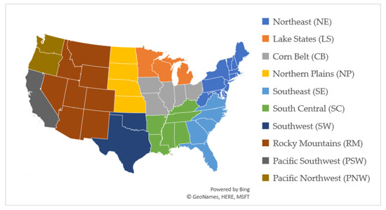
Figure 1.
Regions in the United States (Microsoft product screen shots reprinted with permission from Microsoft Corporation).
In order to incorporate the ODCV phase combination crop yield effects, we calculated the percentage change in average crop yields under each of the seven alternative phase combinations relative to the base case of PDO+TAG+WPWP+ using the calculated regional total effects with PDO+TAG+WPWP+ having the projected yields when all ODCV indicator variables are held at zero. In turn, we computed the average yields and recalibrated the ODCV effects of the eight phase combinations so they were relative to the mean. This information was then used to define the crop yields by region under the eight states of nature where the percentage deviations were applied to the model yields.
3. Results and Discussion: The Value of ODCV Phase Information
In order to find the value of ODCV information, we first found the effects of the ODCV events on the climate variables and, in turn, the effect on crop yields both nationally and regionally. Details about the mean and variance of US crop yields under ODCV can be found in Table S1, national and regional climate effects can be found in Tables S2–S23 of the Supplementary Materials, and yield effects are reported in Tables S24–S34.
The three most commonly occurring events during our study period are PDO−TAG−WPWP−, PDO−TAG+WPWP+, and PDO+TAG+WPWP−, and we will focus discussion on them. We find that nationally for the spring cropping season, PDO−TAG−WPWP− significantly decreases the mean temperature and number of days with temperatures at or above 90 °F and increases the number of days with low temperatures at or below 0 °F all relative to the base case of PDO+TAG+WPWP+. Both of the other two main phase combinations increase the number of days with extreme low temperatures and decrease the total precipitation during the spring cropping season, with PDO−TAG+WPWP+ significantly increasing the number of extremely warm days (DT90) and PDO+TAG+WPWP− significantly decreasing the mean temperature.
Table 3 shows the resultant total effects in national average crop yields. Tables reporting regional effects can be found in Tables S35–S44 of the Supplementary Materials.

Table 3.
Total effect of ODCV phase combinations on national average crop yields in percentage change.
The Table 3 results show that two ODCV phase combinations have negative marginal effects on national corn yields, with the other five having positive effects. Namely when the PDO+TAG+WPWP− phase combination occurs, corn yields are lower by approximately 7% relative to the base case, while PDO−TAG−WPWP− reduces yields by about 3.5%. On the positive side the PDO+TAG−WPWP+ phase combination increases corn yields the most, by about 47.5%. This implies that given ODCV phase information, we might expect farmers to react by planting more or fewer acres of corn in reaction to the associated yield changes.
Similarly, the estimated yields of the other crops react in a mixture of positive and negative ways, with the largest effects occurring under PDO+TAG−WPWP+. Sensitivity is highest for cotton and soybeans and lowest for hay and winter wheat. Note that these results differ by region, with Figure 2, Figure 3, Figure 4, Figure 5, Figure 6, Figure 7 and Figure 8 showing average sensitivity for the crops by region and phase combination and Table 4 showing largest positive, largest negative, and average yield change across the crops by region. Detailed percentage changes for each crop in each region can be found in Tables S45–S51 of the Supplementary Materials.
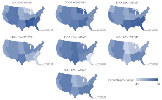
Figure 2.
Percentage changes in corn yields by region for the ODCV phase combinations (Microsoft product screen shots reprinted with permission from Microsoft Corporation).
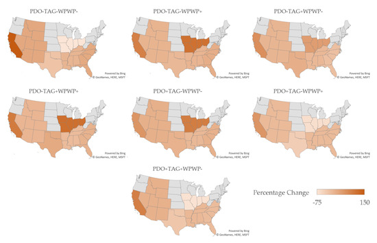
Figure 3.
Percentage changes in cotton yields by region for the ODCV phase combinations (Microsoft product screen shots reprinted with permission from Microsoft Corporation).
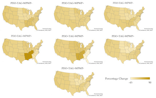
Figure 4.
Percentage changes in hay yields by region for the ODCV phase combinations (Microsoft product screen shots reprinted with permission from Microsoft Corporation).
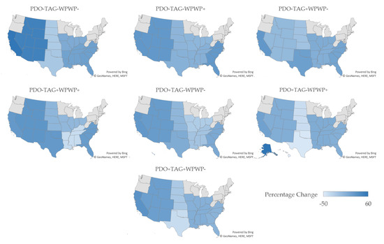
Figure 5.
Percentage changes in sorghum yields by region for the ODCV phase combinations (Microsoft product screen shots reprinted with permission from Microsoft Corporation).
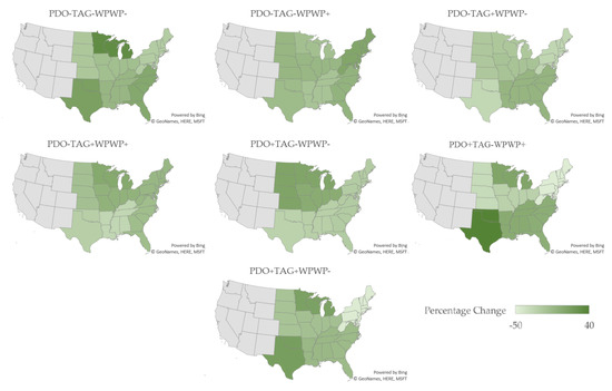
Figure 6.
Percentage changes in soybean yields by region for the ODCV phase combinations (Microsoft product screen shots reprinted with permission from Microsoft Corporation).
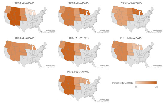
Figure 7.
Percentage changes in spring wheat yields by region for the ODCV phase combinations (Microsoft product screen shots reprinted with permission from Microsoft Corporation).
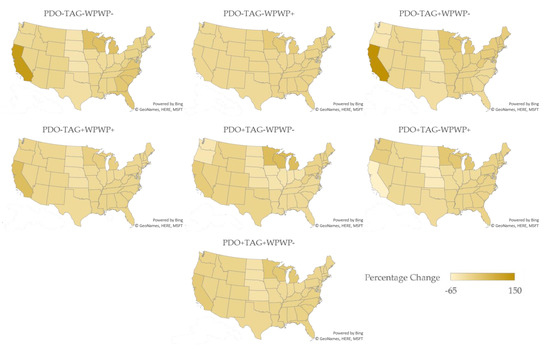
Figure 8.
Percentage changes in winter wheat yields by region for the ODCV phase combinations (Microsoft product screen shots reprinted with permission from Microsoft Corporation).

Table 4.
Average percentage yield change, largest increase, and largest decrease across crops by region.
After obtaining the welfare results, we find that there are positive welfare gains that could be attained by releasing ODCV phenomena phase combination information. Our initial estimates indicate that that the full use of conditional probabilities and associated yields increases welfare by about $86 million annually. Additionally, when perfect information is fully used, the welfare gain is approximately $1.1 billion annually.
The potential welfare gains occur because farmers, livestock producers, processers, and consumers can make adaptive, better performing crop mix, input usage and consumption decisions. One of the big effects is that advanced forecast knowledge of crop yield gains and losses gives opportunities to adjust crop mix and production practices. Table 5 and Table 6 show summaries of some of the main acreage changes from the uninformed case under conditional and perfect information. There we see some regions did not show meaningful changes in acres grown under some cases. However, in the regions discussed below, potential economic gains can be made by adjusting crop acres grown.

Table 5.
Changes in acres planted under conditional information.

Table 6.
Changes in acres planted under perfect information.
3.1. Findings on Adaptation with Conditional Forecasts
When provided with probabilities of ODCV phase combinations for next year that are conditional on this year’s observed phase combination, the modeling framework simulates profit-maximizing farmers in some regions switching their crop mix such that they favor some and reduce others. Table 5 shows the change in crop mix acres. The results indicate that with this type of increased information, net total corn acres increase the most when the previous year’s phase combination was PDO+TAG−WPWP− with a total increase of approximately a half million acres. In contrast, total acres devoted to corn decrease by the largest amount when the previous year’s phase combination is PDO−TAG+WPWP− (a decrease of approximately 2.9 million acres). In contrast, cotton acres are increased the most when the previous year’s phase combination is PDO−TAG−WPWP+, with approximately 512,000 more acres grown. This situation also increases hay acres planted and is expected to increase the number of acres devoted to sorghum. Acres devoted to soybeans are expected to decrease in all scenarios except when the previous year’s phase combination was PDO−TAG−WPWP+ or PDO−TAG+WPWP−. Spring wheat is expected to have the largest increases in acres grown when the previous year’s phase combination was PDO+TAG+WPWP+, while winter wheat is expected to have decreases in acres grown in this scenario (with the largest decrease occurring when the previous year’s phase combination was PDO−TAG−WPWP+).
The largest net increase in total acres grown across all crops is expected to occur when the previous year’s phase combination is PDO+TAG−WPWP+. In this scenario, a net of approximately 698,000 more acres are expected to be utilized than under the base case of no information. In contrast, the largest net decrease in the number of acres planted across all crops examined is expected to occur when the previous year’s phase combination was PDO−TAG+WPWP−, with a total decrease of approximately 566,000 acres expected.
3.2. Findings on Adaptation with Perfect Information
When provided with perfect information on the coming year’s ODCV phase combination, crop mix is again altered. In fact, alterations are larger in the perfect information case (Table 6) than in the conditional information case (Table 5) as outcomes are certain, whereas, in the conditional case, several outcomes were possible.
The PDO+TAG−WPWP+ phase combination induces the largest crop mix change. Hay, sorghum, and spring wheat have the largest expected increases in area planted, while soybeans exhibit the largest decrease during these years. Additionally, when PDO+TAG−WPWP− is projected, corn and hay acres decrease, and cotton acres increase to its largest level. Soybean acres increase the most under PDO−TAG−WPWP+, while winter wheat exhibits its largest decrease. Corn acres increase the most under PDO+TAG+WPWP−, while sorghum exhibits the largest decrease.
Across all crops, perfect information on the occurrence of PDO+TAG+WPWP− leads to the largest increase in acres planted with a total increase of approximately 0.75 million acres. Conversely, knowing that PDO−TAG+WPWP+ will be the coming phase combination leads to approximately 1.5 million fewer acres being planted on net across all crops.
4. Conclusions
ODCV phase combinations are found to significantly alter crop yields and, in turn, given knowledge about likely future phase combinations, stimulate adaptations that are worth between $86 million and $1.1 billion per year depending on forecast accuracy. The estimates were based on econometric and economic analysis. The econometric analysis examined the effects of ODCV phase combinations on climate and, in turn, crop yields. That analysis shows that ODCV phase combinations significantly alter crop yields in a crop- and geographic-specific manner, with some of the effects being as much as 20%.
We did an economic analysis that simulated crop mix, crop production practice, processing, and consumption decisions that are optimal adaptations to the yield effects estimates. These were simulated using a stochastic agricultural sector nonlinear programming model. Responses were simulated to conditional and perfect ODCV phase combination forecasts. We found that when the forecast involved a conditional probability across a range of possible ODCV phase combination outcomes, the adaptive decisions can increase welfare by approximately $86 million annually. We also found that when the forecast perfectly gives next year’s ODCV phase combination, the welfare gains are expected to be about $1.1 billion annually. We also looked at crop mix adjustments and found them to be substantial across the different forecasts.
Overall, we feel the findings of this study suggest that increased spending on the improvement and the release of ODCV phase combination forecasts and the distribution of associated information on ODCV impacts on regional climate and crop yield appears desirable given the potential increases in welfare.
Supplementary Materials
The following are available online at https://www.mdpi.com/2073-4433/11/4/318/s1, Table S1: Mean and Variance of US Yields under ODCV, Table S2: Regression Results for Effect of ODCV Phase Combinations on Spring Climate Variables, Table S3: Regression Results for Effect of ODCV Phase Combinations on Winter Climate Variables, Table S4: Regression Results for ODCV Phase Combination Effects on Spring Climate Variables in Corn Belt, Table S5: Regression Results for ODCV Phase Combination Effects on Winter Climate Variables in Corn Belt, Table S6: Regression Results for ODCV Phase Combination Effects on Spring Climate Variables in Great Plains, Table S7: Regression Results for ODCV Phase Combination Effects on Winter Climate Variables in Great Plains, Table S8: Regression Results for ODCV Phase Combination Effects on Spring Climate Variables in Lake States, Table S9: Regression Results for ODCV Phase Combination Effects on Winter Climate Variables in Lake States, Table S10: Regression Results for ODCV Phase Combination Effects on Spring Climate Variables in Northeast, Table S11: Regression Results for ODCV Phase Combination Effects on Winter Climate Variables in Northeast, Table S12: Regression Results for ODCV Phase Combination Effects on Spring Climate Variables in Pacific Northwest, Table S13: Regression Results for ODCV Phase Combination Effects on Winter Climate Variables in Pacific Northwest, Table S14: Regression Results for ODCV Phase Combination Effects on Spring Climate Variables in Pacific Southwest, Table S15: Regression Results for ODCV Phase Combination Effects on Winter Climate Variables in Pacific Southwest, Table S16: Regression Results for ODCV Phase Combination Effects on Spring Climate Variables in Rocky Mountains, Table S17: Regression Results for ODCV Phase Combination Effects on Winter Climate Variables in Rocky Mountains, Table S18: Regression Results for ODCV Phase Combination Effects on Spring Climate Variables in South Central, Table S19: Regression Results for ODCV Phase Combination Effects on Winter Climate Variables in South Central, Table S20: Regression Results for ODCV Phase Combination Effects on Spring Climate Variables in Southeast, Table S21: Regression Results for ODCV Phase Combination Effects on Winter Climate Variables in Southeast, Table S22: Regression Results for ODCV Phase Combination Effects on Spring Climate Variables in Southwest, Table S23: Regression Results for ODCV Phase Combination Effects on Winter Climate Variables in Southwest, Table S24: Regression Results for Climate and ODCV Phase Combination Effects on US Crop Yields, Table S25: Regression Results for Climate and ODCV Phase Combination Effects on Northeast Crop Yields, Table S26: Regression Results for Climate and ODCV Phase Combination Effects on Lake States Crop Yields, Table S27: Regression Results for Climate and ODCV Phase Combination Effects on Corn Belt Crop Yields, Table S28: Regression Results for Climate and ODCV Phase Combination Effects on Great Plains Crop Yields, Table S29: Regression Results for Climate and ODCV Phase Combination Effects on Southeast Crop Yields, Table S30: Regression Results for Climate and ODCV Phase Combination Effects on South Central Crop Yields, Table S31: Regression Results for Climate and ODCV Phase Combination Effects on Rocky Mountain Crop Yields, Table S32: Regression Results for Climate and ODCV Phase Combination Effects on Southwest Crop Yields, Table S33: Regression Results for Climate and ODCV Phase Combination Effects on Pacific Southwest Crop Yields, Table S34: Regression Results for Climate and ODCV Phase Combination Effects on Pacific Northwest Crop Yields, Table S35: Total Effect of ODCV Phase Combinations on Northeast Crop Yields, Table S36: Total Effect of ODCV Phase Combinations on Lake States Crop Yields, Table S37: Total Effect of ODCV Phase Combinations on Corn Belt Crop Yields, Table S38: Total Effect of ODCV Phase Combinations on Great Plains Crop Yields, Table S39: Total Effect of ODCV Phase Combinations on Southeast Crop Yields, Table S40: Total Effect of ODCV Phase Combinations on South Central Crop Yields, Table S41: Total Effect of ODCV Phase Combinations on Rocky Mountain Crop Yields, Table S42: Total Effect of ODCV Phase Combinations on Southwest Crop Yields, Table S43: Total Effect of ODCV Phase Combinations on Pacific Southwest Crop Yields, Table S44: Total Effect of ODCV Phase Combinations on Pacific Northwest Crop Yields, Table S45. Percentage Changes in Corn Yields by Region, Table S46. Percentage Changes in Cotton Yields by Region, Table S47. Percentage Changes in Hay Yields by Region, Table S48. Percentage Changes in Sorghum Yields by Region, Table S49. Percentage Changes in Soybean Yields by Region, Table S50. Percentage Changes in Spring Wheat Yields by Region, Table S51. Percentage Changes in Winter Wheat Yields by Region.
Author Contributions
Conceptualization, B.A.M.; methodology, B.A.M. and L.A.R.; software, B.A.M. and L.A.R.; validation, L.A.R.; formal analysis, L.A.R.; investigation, L.A.R.; resources, B.A.M.; data curation, L.A.R.; writing—original draft preparation, L.A.R.; writing—review and editing, B.A.M.; visualization, L.A.R.; supervision, B.A.M.; project administration, L.A.R.; funding acquisition, B.A.M. All authors have read and agreed to the published version of the manuscript.
Funding
This research was funded by the U.S. Department of Agriculture National Institute of Food and Agriculture under grant 2011-67003-30213 in the NSF-USDA-DOE Earth System Modelling Program, and by the NOAA Climate Programs Office Sectoral Applications Research Program under grant NA12OAR4310097. The views expressed in this article are only those of the authors and do not necessarily represent the official views of the grantors or any affiliated organizations.
Conflicts of Interest
The funders had no role in the design of the study; in the collection, analyses, or interpretation of data; in the writing of the manuscript, or in the decision to publish the results. The authors declare no conflict of interest.
Appendix A. ODCV Effects on Weather
We examine how the climate variables are influenced by ODCV phenomena by regressing each climate variable on a set of indicator variables for ODCV phase combinations and time trends. Table A1 shows the years associated with each ODCV phase combination.

Table A1.
ODCV Phase Combination Years.
Table A1.
ODCV Phase Combination Years.
| ODCV Phase Combination | Years 1 |
|---|---|
| PDO−TAG−WPWP− | 1965, 1971, 1972, 1974, 1975, 1989, 1991, 1994, 2008 |
| PDO−TAG−WPWP+ | 1959, 1963, 1968, 1973, 1999, 2000, 2009 |
| PDO−TAG+WPWP− | 1955, 1966, 1967, 2001 |
| PDO−TAG+WPWP+ | 1950, 1951, 1952, 1953, 1954, 1956, 1961, 1962, 1964, 1969, 1970, 1990, 2007, 2010 |
| PDO+TAG−WPWP− | 1977, 1984, 1985, 1986, 1993 |
| PDO+TAG−WPWP+ | 1988, 1995, 1996, 2002, 2003 |
| PDO+TAG+WPWP− | 1976, 1978, 1979, 1980, 1982, 1983, 1987, 1992, 1997, 2006 |
| PDO+TAG+WPWP+ | 1957, 1958, 1960, 1981, 1998, 2004, 2005 |
1 Source: Fernandez [36].
Incorporating the ODCV effects was done by defining seven indicator variables for the ODCV phase combinations PDO−TAG−WPWP−, PDO−TAG−WPWP+, PDO−TAG+WPWP−, PDO−TAG+WPWP+, PDO+TAG−WPWP−, PDO+TAG−WPWP+, and PDO−TAG+WPWP+ with the eighth phase combination PDO+TAG+WPWP+ being the base case. Descriptions of the climate variables are given in Section 2.1 of the main text. The estimation was done using clustered standard errors with state fixed effects yielding state specific estimates. Equation (A1) shows the specification used for the linear regression with representing a climate variable (DT90, DT00, DP10, TPCP, or MNTM for the spring and winter cropping season) in location at time , representing the set of parameters corresponding to the regression that are to be estimated, and representing the error term. The indicator variables represented by each of the ODCV phase combination names take either a value of 1 if the event was present in that year or 0 if the event was not present that year.
Tables S2–S23 in the Supplementary Materials show the results by region. This information is utilized in later steps to find the total yield effects.
Appendix B. Estimating Climate and ODCV Effects on Crop Yields
Now we turn to the yield estimations, examining the effects of the climate variables and the ODCV phase combinations. We regress yield for each crop in each region on the climate variables discussed previously, the set of indicator variables for ODCV phase combinations and time trends. The general specification can be seen in Equation (A2) where is the per acre yield in location for crop at time and is the set of parameters corresponding to the regression. The climate and indicator variables are as discussed above.
State level crop yield data for corn, cotton, hay, sorghum, soybeans, spring wheat, and winter wheat are used. Lagged yields were included in the estimations where stationarity issues were detected. Additionally, the number of planted acres () is included in the estimations where available to account for potential planted acres density effects [37] and any other potential effects from planting scale. Squared time and climate variables are also included as previous studies have determined nonlinear relationships between climate attributes and crop yields [38,39,40]. Tables S24–S34 in the Supplementary Materials contain the regression results.
In order to calculate the total marginal effect of the ODCV phase combinations, we considered both the direct effect of the ODCV indicator variables plus the indirect effects through changes in the climate variables and, in turn, the effects of those altered climate variables on yields as done and explained in Jithitikulchai et al. [16]. As Equation (A2) is a function of Equation (A1), the total marginal effect of the ODCV phase combination can be calculated by:
This number can then be used in conjunction with the average crop yields to determine the percentage change in crop yields from each of the phase combinations.
References
- Chen, C.C.; McCarl, B.A.; Adams, R.M. Economic implications of potential ENSO frequency and strength shifts. Clim. Chang. 2001, 49, 147–159. [Google Scholar] [CrossRef]
- Hammer, G.L.; Hansen, J.W.; Phillips, J.G.; Mjelde, J.W.; Hill, H.S.J.; Love, H.A.; Potgieter, A. Advances in applications of climate prediction in agriculture. Agric. Syst. 2001, 70, 515–553. [Google Scholar] [CrossRef]
- Mantua, N.J.; Hare, S.R. The pacific decadal oscillation. J. Oceanogr. 2002, 58, 35–44. [Google Scholar] [CrossRef]
- Partin, J.W.; Cobb, K.M.; Adkins, J.F.; Clark, B.; Fernandez, D.P. Millennial-scale trends in West Pacific Warm Pool hydrology since the last glacial maximum. Nature 2007, 449, 452–455. [Google Scholar] [CrossRef] [PubMed]
- Grossman, I.; Klotzbach, P.J. A review of North Atlantic modes of natural variability and their driving mechanisms. J. Geophys. Res. Atmos. 2009, 114. [Google Scholar] [CrossRef]
- Mantua, N.J.; Hare, S.R.; Zhang, Y.; Wallace, J.M.; Francis, R.C. A Pacific interdecadal climate oscillation with impacts on salmon production. Bull. Am. Meteorol. Soc. 1997, 78, 1069–1079. [Google Scholar] [CrossRef]
- Nigam, S.; Barlow, M.; Berbery, E.H. Analysis links Pacific decadal variability to drought and streamflow in United States. EOS Trans. Am. Geophys. Union 1999, 80, 621–625. [Google Scholar] [CrossRef]
- Miller, A.J.; Schneider, N. Interdecadal climate regime dynamics in the North Pacific Ocean: Theories, observations and ecosystem impacts. Prog. Oceanogr. 2000, 47, 355–379. [Google Scholar] [CrossRef]
- Mehta, V.M.; Rosenberg, N.J.; Mendoza, K. Simulated impacts of three decadal climate variability phenomena on dryland corn and wheat yields in the Missouri River Basin. Agric. For. Meteorol. 2012, 152, 109–124. [Google Scholar] [CrossRef]
- Lukas, R.; Lindstrom, E. The mixed layer of the Western Equatorial Pacific Ocean. J. Geophys. Res. Ocean 1991, 96, 3343–3357. [Google Scholar] [CrossRef]
- Huang, B.; Mehta, V.M. Response of the Indo-Pacific Warm Pool to interannual variations in net atmospheric freshwater. J. Geophys. Res. Ocean 2004, 109. [Google Scholar] [CrossRef]
- Good, P.; Lowe, J.A.; Rowell, D.P. Understanding uncertainty in future projections for the Tropical Atlantic: Relationships with the unforced climate. Clim. Dyn. 2009, 32, 205–218. [Google Scholar] [CrossRef]
- Murphy, J.; Kattsov, V.; Keenlyside, N.; Kimoto, M.; Meehl, G.; Mehta, V.M.; Pohlmann, H.; Scaife, A.; Smith, D. Towards prediction of decadal climate variability and change. Procedia Environ. Sci. 2010, 1, 287–304. [Google Scholar] [CrossRef]
- Fernandez, M.A.; Huang, P.; McCarl, B.A.; Mehta, V.M. Value of decadal climate variability information for agriculture in the Missouri River Basin. Clim. Chang. 2016, 139, 517–533. [Google Scholar] [CrossRef]
- Ding, J. Three Essays on Climate Variability, Water and Agricultural Production. Ph.D. Thesis, Texas A&M University, College Station, TX, USA, 2014. [Google Scholar]
- Jithitikulchai, T.; McCarl, B.A.; Wu, X.M. Decadal climate variability impacts on climate and crop yields. J. Agric. Appl. Econ. 2019, 51, 104–125. [Google Scholar] [CrossRef]
- Vallorani, R.; Bartolini, G.; Betti, G.; Crisci, A.; Gozzini, B.; Grifoni, D.; Iannuccilli, M.; Messeri, A.; Messeri, G.; Morabito, M.; et al. Circulation type classifications for temperature and precipitation stratification in Italy. Int. J. Climatol. 2018, 38, 915–931. [Google Scholar] [CrossRef]
- Solow, A.R.; Adams, R.M.; Bryant, K.J.; Legler, D.M.; O’Brien, J.J.; McCarl, B.A.; Nayda, W.I.; Weiher, R.F. The value of improved ENSO prediction to US agriculture. Clim. Chang. 1998, 39, 47–60. [Google Scholar] [CrossRef]
- Mjelde, J.W.; Hill, H.S.J. The effect of the use of improved climate forecasts on variable costs, input usage, and production. Agric. Syst. 1999, 60, 213–225. [Google Scholar] [CrossRef]
- Chen, C.C.; McCarl, B.A. The value of ENSO information to agriculture: Consideration of event strength and trade. J. Agric. Resour. Econ. 2000, 25, 368–385. [Google Scholar]
- Hill, H.S.J.; Mjelde, J.W.; Rosenthal, W.; Love, H.A.; Fuller, S.W. Comparing the value of Southern Oscillation index-based climate forecast methods for Canadian and US wheat producers. Agric. For. Meteorol. 2000, 100, 261–272. [Google Scholar] [CrossRef]
- Chen, C.C.; McCarl, B.A.; Hill, H.S.J. Agricultural value of ENSO information under alternative phase definition. Clim. Chang. 2002, 54, 305–325. [Google Scholar] [CrossRef]
- Letson, D.; Podestá, G.P.; Messina, C.D.; Ferreyra, R.A. The uncertain value of perfect ENSO phase forecasts: Stochastic agricultural prices and intra-phase climatic variations. Clim. Chang. 2005, 69, 163–196. [Google Scholar] [CrossRef]
- Kim, M.K.; McCarl, B.A. The agricultural value of information on the North Atlantic Oscillation: Yield and economic effects. Clim. Chang. 2005, 71, 117–139. [Google Scholar] [CrossRef]
- Tack, J.B.; Harri, A.; Coble, K.C. More than mean effects: Modeling the effects of climate on the higher order moments of crop yields. Am. J. Agric. Econ. 2012, 94, 1037–1054. [Google Scholar] [CrossRef]
- Lobell, D.B.; Asseng, S. Comparing estimates of climate change impacts from process-based and statistical crop models. Environ. Res. Lett. 2017, 12, 015001. [Google Scholar] [CrossRef]
- Attavanich, W.; McCarl, B.A. How is CO2 affecting yields and technological progress? A statistical analysis. Clim. Chang. 2014, 124, 747–762. [Google Scholar] [CrossRef]
- Tack, J.B.; Ubilava, D. Climate and agricultural risk: Measuring the effect of ENSO on US crop insurance. Agric. Econ. 2015, 46, 245–257. [Google Scholar] [CrossRef]
- USDA/NASS QuickStats Ad-Hoc Query Tool. Available online: https://quickstats.nass.usda.gov/ (accessed on 1 May 2017).
- NOAA Data Access. Available online: https://www.ncdc.noaa.gov/data-access (accessed on 27 June 2018).
- Baron, R.M.; Kenny, D.A. The moderator-mediator variable distinction in social psychological research: Conceptual, strategic, and statistical considerations. J. Personal. Soc. Psychol. 1986, 51, 1173–1182. [Google Scholar] [CrossRef]
- Huang, P.; McCarl, B.A. Estimating decadal climate variability effects on crop yields: A bayesian hierarchical approach. In Proceedings of the Agricultural & Applied Economics Association’s 2014 AAEA Annual Meeting, Minneapolis, MN, USA, 27–29 July 2014. [Google Scholar]
- Adams, R.M.; Bryant, K.J.; McCarl, B.A.; Legler, D.M.; O’Brien, J.J.; Solow, A.R.; Weiher, R.F. Value of improved long-range weather information. Contemp. Econ. Policy 1995, 13, 10–19. [Google Scholar] [CrossRef]
- Beach, R.H.; Adams, D.; Alig, R.; Baker, J.; Latta, G.S.; McCarl, B.A.; Murray, B.C.; Rose, S.K.; White, E. Model Documentation for the Forest and Agricultural Sector Optimization Model with Greenhouse Gases (FASOMGHG); RTI International: Research Triangle Park, NC, USA; Available online: http://www.cof.orst.edu/cof/fr/research/tamm/FASOMGHG_Model_Documentation_Aug2010.pdf (accessed on 2 June 2016).
- Lambert, D.K.; McCarl, B.A.; He, Q.; Kaylen, M.S.; Rosenthal, W.; Chang, C.C.; Nayda, W.I. Uncertain yields in sectoral welfare analysis: An application to global warming. J. Agric. Appl. Econ. 1995, 27, 423–436. [Google Scholar] [CrossRef][Green Version]
- Fernandez, M.A. Decadal Climate Variability: Economic Implications in Agriculture and Water in the Missouri River Basin. Ph.D. Thesis, Texas A&M University, College Station, TX, USA, 2013. [Google Scholar]
- Lyon, D.J. How do plant populations affect yield. In Press Release from Panhandle Research and Extension Center; Agricultural Research Division of IANR: Lincoln, Nebraska, 2009; Volume 19. [Google Scholar]
- Mendelsohn, R.O.; Nordhaus, W.D.; Shaw, D. The impact of global warming on agriculture: A Ricardian analysis. Am. Econ. Rev. 1994, 84, 753–771. [Google Scholar]
- Schlenker, W.; Roberts, M.J. Nonlinear temperature effects indicate severe damages to US crop yields under climate change. Proc. Natl. Acad. Sci. USA 2009, 106, 15594–15598. [Google Scholar] [CrossRef] [PubMed]
- Huang, P. Three Essays on Economic and Societal Implication of Decadal Climate Variability and Fishery Management. Ph.D. Thesis, Texas A&M University, College Station, TX, USA, 2015. [Google Scholar]
© 2020 by the authors. Licensee MDPI, Basel, Switzerland. This article is an open access article distributed under the terms and conditions of the Creative Commons Attribution (CC BY) license (http://creativecommons.org/licenses/by/4.0/).