Abstract
Ionospheric structure usually changes dramatically during a strong geomagnetic storm period, which will significantly affect the short-wave communication and satellite navigation systems. It is critically important to make accurate ionospheric predictions under the extreme space weather conditions. However, ionospheric prediction is always a challenge, and pure physical methods often fail to get a satisfactory result since the ionospheric behavior varies greatly with different geomagnetic storms. In this paper, in order to find an effective prediction method, one traditional mathematical method (autoregressive integrated moving average—ARIMA) and two deep learning algorithms (long short-term memory—LSTM and sequence-to-sequence—Seq2Seq) are investigated for the short-term predictions of ionospheric TEC (Total Electron Content) under different geomagnetic storm conditions based on the MIT (Massachusetts Institute of Technology) madrigal observation from 2001 to 2016. Under the extreme condition, the performance limitation of these methods can be found. When the storm is stronger, the effective prediction horizon of the methods will be shorter. The statistical analysis shows that the LSTM can achieve the best prediction accuracy and is robust for the accurate trend prediction of the strong geomagnetic storms. In contrast, ARIMA and Seq2Seq have relatively poor performance for the prediction of the strong geomagnetic storms. This study brings new insights to the deep learning applications in the space weather forecast.
1. Introduction
It is well known that geomagnetic storms and substorms substantially disturb the Earth’s magnetosphere and ionosphere [1,2]. Geomagnetic storms are often associated with the impact of Earthward directed CMEs (Coronal Mass Ejections) and coronal holes [3,4], and the substorms are associated with the magnetic reconnection in the Earth’s magnetotail [5,6,7,8]. These accelerated particles can precipitate into the ionosphere [9] and substantially modify the behavior of polar ionosphere. Meanwhile, the disturbed high-latitude convection and enhanced Joule heating will also significantly change the dynamics of the ionosphere [10].
With the rapid development of modern technology, human’s daily life has already dramatically relied on the various satellite systems operating in the ionosphere. However, during a geomagnetic storm, the physical structure and chemical composition of the ionosphere will change drastically according to the real-time space environment [11,12,13], causing the destruction of the propagation environment of radio waves in the ionosphere. It may ultimately result in short wave communication interruption, satellite navigation errors or other related satellite-to-ground communication failures. Therefore, it is very important to understand the behavior of the ionosphere and achieve accurate predictions during geomagnetic storms. In the last several decades, research on ionospheric storms has been carried out and made very deep and comprehensive progress on the ionospheric storm simulation, observation analysis, and data processing [10,14,15,16,17,18]. These studies can provide the basic trend of ionospheric variation, but the ionospheric behaviors during a geomagnetic storm are still too difficult to be predicted effectively with high precision. On the other hand, the physical mechanisms exhibited by the effect of different geomagnetic storms on the ionosphere often show huge differences, and some strong nonlinear processes have emerged, which finally bring challenges to the traditional theoretical modelling and corresponding predictions [19,20,21,22].
Due to the tremendous increase in satellite projects and the accumulation of observations, the era of big data has arrived, which makes it possible to solve some difficult challenges and problems. The emergence of high-performance GPUs (Graphics Processing Units) has also stimulated the rapid application of deep learning algorithms in artificial intelligence. Correspondingly, these deep learning algorithms can perform classification tasks directly from image, text, or time series sound data. They can achieve incredible accuracy, sometimes even beyond human performance [23]. ARIMA (autoregressive integrated moving average) is one of the most widely used methods for time series forecasting, and it has been widely used in space physics [24]. Zhang et al. [25] used the ARIMA model to make a short-term prediction of ionospheric TEC, whose prediction performance and results can be a meaningful reference for comparison. Moreover, deep learning algorithms train a model by using a large number of labeled datasets and a neural network architecture including many layers, thereby extracting a large number of parameters and features from the data to identify, classify, and predict an important phenomenon, behaviors, etc.
Recently, some related methods of deep learning have been applied very quickly to some research fields of space science to compare with the traditional observations or simulations. Le et al. [26] have shown that deep learning is very good at discovering complex structures in high-dimensional data. Xenos et al. [27] used neural networks techniques to predict foF2 and M(3000)F2. Oyeyemi et al. [28] developed a neural network model for foF2 prediction. Their results from NRTNN (Near-Real Time global foF2 Neural Network) could predict foF2 in near real-time with about 1 MHz RMSE difference anywhere on the globe. These provided real-time data that is available at the four control stations. Mandrikova et al. [29] suggested a technique of ionospheric parameter modelling and analysis based on combining the wavelet transform with ARIMA models to predict foF2 and TEC. Their method facilitated ionospheric dynamic mode analysis and proved to be efficient for making predictions with a time advance equal to 5 hours. Sun et al. [30] presented a good prediction method for ionospheric TEC data in different space weather conditions by using a long short-term memory (LSTM) network. The experimental results showed that their proposed LSTM model could achieve a more stable convergence tendency and less RMS error than their multilayer perceptron (MLP) result. Cherrier et al. [31] proposed an LSTM-based sequence-to-sequence (Seq2Seq) model for the TEC prediction, which also indicated that the deep learning algorithms have good potential for space weather prediction. Gruet et al. [32] used the LSTM method combined with Gaussian process model to establish a probabilistic prediction for the geomagnetic index Dst. This model can predict the Dst index for up to 6 hours. Tan et al. [33] also applied LSTM to the prediction of Kp geomagnetic index. The corresponding RMSE (Root Mean Square Error, the standard deviation of the residuals, a measure of how spread out these residuals are) and MAE (Mean Absolute Error which is the average over the verification sample of the absolute values of the differences between forecast and the corresponding observation) are smaller than those of other models, and the correlation coefficient is good enough for Kp forecasting. Chen et al. [34] proposed an improved generative adversarial deep learning algorithm (RDCGAN) to directly train the global TEC map which contains partial missing data. The RDCGAN model can effectively extract and learn the detailed characteristics from the spatial distribution of TEC maps and can automatically recover the important missing part. It can be noted that these deep learning algorithms have made fast and significant progress in space weather predictions.
Although these mentioned deep learning methods already showed their valid prediction results in ionospheric TEC data, the effectiveness and robustness of these methods under disturbed geomagnetic conditions, e.g., geomagnetic storm, still need to be validated and improved. The effects of geomagnetic conditions on the deep learning predictions are worthy of statistical discussions. In this paper, we adopted three prediction methods to present detailed comparisons of TEC data prediction during different geomagnetic storms based on statistical analysis of 15 years’ TEC data. One method is a traditional time series modeling technique, ARIMA. The other two methods are deep learning methods, long short-term memory (LSTM) and Seq2Seq. The goal of this paper is to predict ionospheric TEC during a geomagnetic storm, which belongs to a short-term prediction research. Under the extreme condition, the performance limitation of these methods can be found. When the storm is stronger, the effective prediction horizon of the methods will be shorter.
The rest of this paper is organized as follows. The details of the ARIMA, LSTM, and Seq2Seq algorithms are briefly introduced in Section 2. Section 3 proposes the comparisons for three algorithms under geomagnetic quiet period, great storm, and strong major storm, respectively. In addition, the statistical analysis of 55 storm events that occurred from 2001 to 2016 is presented based on the correlation analysis. Finally, the conclusion and directions for future work are summarized in Section 4.
2. TEC Prediction Methods
2.1. ARIMA
ARIMA is a famous time series prediction method introduced by Box and Jenkins in the early 1970s [35]. The main formulas of ARIMA are as follows:
where denotes a smooth time series obtained after d-differentiating from the non-stationary data, and d is a non-seasonal difference order in Formula (1). After the data is differentiated (the first formula), it is subjected to an autoregressive moving average process (the second formula), which contains autoregressive (AR) and moving average (MA) processes. Between them, the positive terms are AR processes, while the negative terms are MA processes. The corresponding non-negative integer p is the autoregressive order, and q is the moving average order. are the regression coefficients, are the moving average coefficients, and is a Gaussian white noise. According to the settings of the parameters p, d, and q, the original ARIMA model can be applied to different forms of time series predictions.
On the other hand, it should be noted that the ionospheric TEC has periodic variations in various scales (annual, seasonal, and diurnal), which requires a seasonal model of ARIMA. It not only needs the basic parameters (p, d, q), but also requires the corresponding seasonal parameters P (seasonal autoregressive order), D (seasonal difference order), Q (seasonal moving average order), and m (number of observations per year).
A seasonal ARIMA (p, d, q) (P, D, Q) m model (without a constant, period m) can be written as
where is the white noise process; is the series; is the p-order non-seasonal autoregressive coefficient; is the P-order seasonal autoregressive coefficient; is the d-order non-seasonal differential coefficient; is the D-order seasonal differential coefficient; is the q-order non-seasonal moving average coefficient; and is the Q-order seasonal moving average coefficient, respectively (lowercase definitions of these coefficients can be found in Box et al. [35]). Generally, the optimal prediction effect should be obtained by adjusting the prediction model several times. In this work, after testing these parameters, we found the optimal prediction performance and the lowest AIC (Akaike information criterion) when p = 1, d = 0, and q = 1. The corresponding seasonal parameters were P = 3, D = 1, Q = 1, and m = 12. The detailed prediction results are shown in Section 3.
However, the ARIMA method is essentially a linear model so that it is not capable of accurate prediction for large observational time series datasets with strong nonlinearity. Yi et al. [36] used transportation big data to build the nonlinear prediction model of traffic conditions by deep learning neural network which can obtain very high accuracy, around 99%. Wang et al. [37] used big system data to build a nonlinear deep learning model for spatiotemporal in cellular network. Zhang et al. [38] made a survey to study the nonlinear modeling technique of deep learning for various big data applications. In this regard, deep learning algorithms hold great potential to improve the prediction performance.
2.2. LSTM and Seq2Seq
Recently, deep learning algorithms have begun to be widely used because of their strong nonlinear factor effects on the network. Here, we adopted the LSTM and Seq2Seq methods based on the recurrent neural network (RNN) algorithm. They have a certain memory function due to the recurrent structure of the traditional RNN and are good at training time series data [39,40]. However, the traditional RNN does not deal well with a long-term dependency problem [41]. The main reason is that gradient vanishing happens due to the multiplication effect in the gradient backpropagation [42]. In order to predict a longer sequence, LSTM was introduced as an improved version of RNN by Hochreiter et al. [43].
Figure 1 presents the framework diagrams of the basic RNN and LSTM models. The main difference is the internal structure of the hidden layer in the recurrent unit A indicated by the dashed box. The recurrent structure of the LSTM consists of three gates (input, forget, output) and a hidden state called ’cell state’, which can store or transfer information and determine the output of the hidden layer. These gates are used to keep or forget the computation information and control the cell state. Usually, we can use sigmoid as the activation function in the gates, while the inputs and cell states are converted using a tanh function.
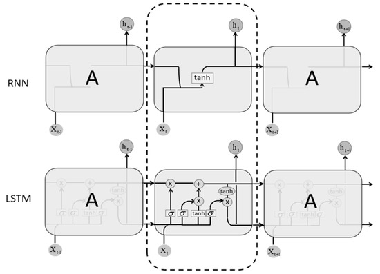
Figure 1.
The model structure diagram of the traditional recurrent neural network (RNN) (top) and long short-term memory (LSTM) (bottom).
In our experiments, we need to construct the input sequence (TEC value) into a dataset that is suitable for training the model (including set a window size). Due to the length of TEC during different magnetic storm period being different, the training dataset and testing dataset are split from the dataset according to the proportion of the prediction period length to the total data set. Table 1 provides the parameters and hyperparameters of LSTM in our experiments.

Table 1.
Parameters and hyperparameters of LSTM.
On the other hand, the original RNN requires that the input sequence be the same length as the output sequence, which makes it impossible to solve a problem such as mechanical translation. The sequence-to-sequence model is also an important variant of basic RNN. Its advantage is that the input sequence and the output sequence can be of unequal length, and it can be seen as a network of encoder–decoder structures. It should be noted that the encoder and decoder structures are equivalent to an RNN. The encoder structure first encodes the input data into a context vector C (content), while the decoder structure turns this fixed-length vector C into a signal sequence of a variable-length target.
Figure 2 shows the structure diagram of the Seq2Seq model [44,45]. are the basic recurrent units representing the RNN. In the encoder process, we input the data vector form into the RNN in sequence, and the current implicit vectors are combined to get the hidden vector at the next moment. The hidden vector obtained at the end of the encoding phase is passed to the vector content and then passed to the decoder unit. In the decode process, the output of the current moment is obtained by decoding the C vector and combining with the current hidden vector.
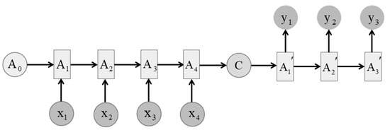
Figure 2.
The structure diagram of the sequence-to-sequence (Seq2Seq) model.
It is necessary to set the sequence length of the input and output before building the model. In every single case, we set the output sequence length as long as the label of testing dataset, the sequence length of the input and output are important basis for dividing training dataset and test dataset. The sequence length of the input and output also decides the input sequence length of the encoder and the output sequence length of the decoder. Table 2 provides the parameters and hyperparameters of Seq2Seq in our experiments.

Table 2.
Parameters and hyperparameters of Seq2Seq.
3. Simulation Results and Discussions
3.1. Data Description
TEC data is one of the important parameters in the ionosphere, which can reflect the ionospheric variation in different geophysical conditions. IGS (International GNSS Service) TEC data have fewer missing data points, while they have good quality [46,47] and long-term global observations; therefore, it is particularly suitable for monitoring changes in the spatiotemporal morphology of the ionosphere. In this paper, we adopted the TEC data from 2001 to 2016 observed by the MIT madrigal for the algorithm training and modeling, which can be downloaded from the following website (http://cedar.openmadrigal.org/ftp/) [48].
In this paper, the training data is obtained from MIT TEC data and has been transformed into grids with meshes of 64 × 64 size. Then we selected one of the grids for our TEC prediction, so that the location of the region is exactly the grid in the region of 138° E, 57° N, the size of the region is that of one grid (the size is 5.625° in longitude and 2.8125° in latitude). In Figure 3, the red rectangle is our chosen region, the gray area denotes missing data, and the white dots denote the GPS stations. As shown in the red box in Figure 3, there are two GPS stations around the chosen grid ensuring that the amount of missing data is within a reasonable range. It is obvious that the missing data is less the more GPS stations are located in that area, and the best data quality is located in the region with most GPS stations. Though the number of the GPS stations of our chosen area is not large, TEC data missing is a common issue in the global observation (a large number of missing values can be seen in the ocean area in Figure 3) which provides negative effects on the prediction performance of all methods. Thus, in order to prove that these methods can be easily applicable in most regions, we believe this region (138° E, 57° N) is a reasonable choice to test these methods (ARIMA, LSTM, Seq2Seq) we chose.
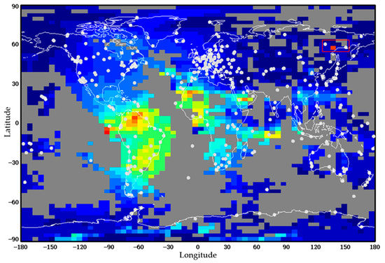
Figure 3.
Region of data selection on a TEC (Total Electron Content) map.
All of the TEC data shown in the following sections are the averaged TEC over the local region, including the training data and test data of our deep learning model. Actually, the size of the local region is 5.625° in longitude and 2.8125° in latitude, and its position is exactly the grid in the region of 138° E, 57° N. Hence, the TEC data is calculated by averaging same TEC data of this region.
The time interval of the training TEC data is two years before our prediction date. For example, if we want to predict TEC data from 1 June 2008 to 8 June 2008, the TEC observations from 31 May 2006 to 31 May 2008 will be the training data. For a given local region, TEC data missing depends on the number of the GPS stations. In this paper, the chosen region is where the number of the GPS stations is at an average level. In such a case, the quality of data is also at an average level. Since the training data varies with different prediction date, the number of the geomagnetic storms is also dynamic. However, the three prediction algorithms use exactly the same training data to build the prediction model; hence, their comparison is reasonable.
Furthermore, since all three methods require a part of the data to train the model, we selected the data about 2 years before the forecast data as the training data. The prediction effects of these obtained models were carefully tested under different geomagnetic activity conditions. Geomagnetic storms can be categorized in terms of geomagnetic activity index (Dst) according to Gonzalez et al. [49]. Major (intense or great) storms can be classified as the minimum Dst (Dstmin) of −100 nT or less, so that 55 major storm cases have been selected. Furthermore, Dstmin of −250 nT or less will be further classified as strong major storm in this research.
3.2. Prediction Analysis
Figure 4 gives an example of three model predictions of TEC variation during the geomagnetic quiet period from 25 February to 5 March 2005. During this period, the level of geomagnetic activity is very low so the range of the Dst index is −20 nT < Dst < 20 nT (Figure 4g). Figure 4a,c,e shows the measured TEC data (black) and the predicted TEC data (red) by the ARIMA, LSTM, and Seq2Seq methods respectively. It can be noted that the measured ionospheric TEC variations are relatively stable and have diurnal variation characteristics (see black lines). The predictions from all three methods (see the red lines have achieved satisfactory results and are basically consistent with the observations. In this event, the correlation coefficients between the observations and predictions are 0.921, 0.891, and 0.836 for the ARIMA, LSTM, and Seq2Seq, respectively. Moreover, it is obvious that the ARIMA and Seq2Seq can show more error peaks, but the LSTM performance is smoother. The peaks of the Seq2Seq are a little higher than those of the other two methods, especially at the daytime.
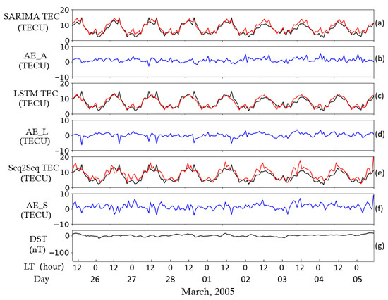
Figure 4.
TEC observation and model predictions during the geomagnetic quiet period from 25 February to 5 March 2005. Panels (a), (c), and (e) are the measured TEC data (black) and the predicted TEC data (red) by the autoregressive integrated moving average (ARIMA), LSTM, and Seq2Seq methods. Panels (b), (d), and (f) are the absolute errors (blue) between predicted TEC and actual TEC. Panel (g) is the geomagnetic disturbance index Dst.
In order to verify the effects of the three prediction models by the different intensity of geomagnetic storms, we then tested the prediction performance under moderate geomagnetic storm conditions. Figure 5 shows an event that occurred from 31 December 2015 to 4 January 2016, and has an identical format to Figure 5 except that minimum Dst = −110 nT.
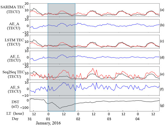
Figure 5.
The TEC measurements and predictions under a major geomagnetic storm from 31 December 2015 to 4 January 2016. All panels have identical format to Figure 4. Panels (a), (c), and (e) are the measured TEC data (black) and the predicted TEC data (red) by the autoregressive integrated moving average (ARIMA), LSTM, and Seq2Seq methods. Panels (b), (d), and (f) are the absolute errors (blue) between predicted TEC and actual TEC. Panel (g) is the geomagnetic disturbance index Dst, and minimum Dst = −110 nT.
It can be seen that during the storm period around 1 January 2016, the actual daily variation of the measured TEC data is significantly lower than those observations before and after this moderate storm (indicated by the shadow region). This response also affects the prediction profiles of all three methods which vary significantly and present a large deviation from the original TEC observation. The predictions from ARIMA and LSTM are much better than those of Seq2Seq since the ARIMA and LSTM obtained smaller RMSE than the Seq2Seq (ARIMA is 1.779; LSTM is 1.484, and Seq2Seq is 3.862). It is very clear that Seq2Seq results contain too many unreal TEC peaks. The predictions from ARIMA and LSTM are much better than those of Seq2Seq (ARIMA and LSTM get smaller RMSE than Seq2Seq, RMSE: ARIMA gets 1.779, LSTM gets 1.484, while Seq2Seq 3.862), since the Seq2Seq results contain too many unreal TEC peaks. The reason is mainly caused by the prediction instability of Seq2Seq and the corresponding correlation coefficient is only 0.583, the prediction performance of Seq2Seq is not always in a good state; sometimes results of Seq2Seq show more error peaks than the others, as can also be clearly seen from Figure 6. Further comparisons between ARIMA and LSTM reveal that the ARIMA result shows large deviations at nighttime, while LSTM performs better consistently. It also suggests a more accurate prediction from LSTM at the low level of TEC variation (this effect can also be seen in Figure 4). Correspondingly, LSTM has a higher correlation coefficient of 0.837, while ARIMA has 0.774. Therefore, it can be seen that the geomagnetic storm is a kind of interference that can significantly affect the variation of the ionospheric background, which makes it difficult to predict the sudden and sharp changes in ionosphere data. Different methods begin to show performance differences.
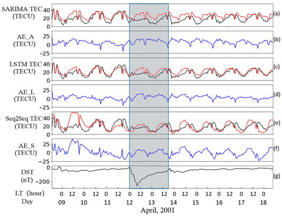
Figure 6.
The TEC measurements and predictions under a strong major geomagnetic storm from 8 April to 18 April 2001. All panels have an identical format to Figure 4. Panels (a), (c), and (e) are the measured TEC data (black) and the predicted TEC data (red) by the autoregressive integrated moving average (ARIMA), LSTM, and Seq2Seq methods. Panels (b), (d), and (f) are the absolute errors (blue) between predicted TEC and actual TEC. Panel (g) is the geomagnetic disturbance index Dst, and minimum Dst = −271nT.
Furthermore, it is necessary to verify the prediction effect of the LSTM under the condition of strong major geomagnetic storms. Figure 6 illustrates the TEC observation and model predictions under a super geomagnetic storm whose minimum value of Dst index is close to −300 nT. The main and recovery phase of the storm occurred from 12 April to 15 April 2001. The prediction results of the three methods show significant differences in the shadow region.
It is very clear that all prediction results have more disturbance compared with the measured value. As shown in Figure 6, the absolute errors of all predictions (blue line) are significant during the geomagnetic storm, and they are very dynamic over time. The TEC profile from the traditional ARIMA method is higher than the original TEC both at daytime and nighttime during the main and recovery phase of this strong major storm. In such a case, the correlation coefficient of the ARIMA is 0.615. It is worth noticing that the prediction profile from the LSTM has less deviation than those from the other two methods, especially after the recovery phase of this super storm. It then has the highest correlation coefficient of 0.721. However, it can be noted that the Seq2Seq method performs better prediction profile when the Dst index is large. During the storm-time, RMSE of the three models are the following: ARIMA—12.568; LSTM—8.775; Seq2Seq—6.352. However, the prediction effect of Seq2Seq is still unstable before and after geomagnetic storm. On 9 April, a very large prediction error occurred (RMSE around this day (9 April) is 22.532), which is similar to the result under major geomagnetic storm in Figure 5e. Since Seq2Seq is more sensitive to the short-term TEC feature than other algorithms during the training process, its prediction is easily affected by the variation of measured TEC. In addition, the positions of the predicted TEC peaks are shifted backward in time during and after the recovery phase. This kind of phase error finally makes the correlation coefficient only 0.396 in this whole event.
Generally, the qualitative analysis shows that the performance of the three prediction methods is significantly affected by the geomagnetic storm. The detailed relationship between the stability of the prediction method and the intensity of the geomagnetic storm in the TEC prediction should be addressed by further statistical analysis.
3.3. Statistical Analysis
In this section, 55 ionospheric TEC datasets of geomagnetic storm events are selected from 2001 to 2016 observed by the MIT madrigal when the minimum Dst value is less than −100 during the main phase of the 55 geomagnetic storms.
Figure 7 illustrates the average of the root mean squared error () between the observed and predicted values against the minimum Dst index of the main phase for each magnetic storm event. is calculated by averaging TEC RMSE of all the magnetic storm events. Every event means a whole period of geomagnetic storm (including initial, main, and recovery phase) which is represented by a cross. It is obvious that the LSTM method achieves the smallest average value of the RMSE and has the best prediction performance. When a super geomagnetic storm (Dstm ≤ −250 nT) occurs, its root mean square error can be controlled below 10 TECU. As for a moderate geomagnetic storm (−100 nT ≤ Dstm ≤ −150 nT), the LSTM prediction can generally obtain a root mean square around 5 TECU. Similar to the previous case study in Figure 4 and Figure 5, the Seq2Seq performs the worst prediction, and the average RMSE is 6.88. Whether it is a major or strong major geomagnetic storm, its performance becomes very unstable. ARIMA, as a traditional time series prediction method, shows relatively stable predictions and its average RMSE is 5.79, which is significantly better than the Seq2Seq, but worse than LSTM. Therefore, the LSTM method presents the best prediction accuracy of the three methods.
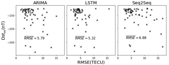
Figure 7.
The average of the root mean square error () between the observed and predicted values (x-axis) against the minimum Dst index of the main phase (y-axis) for the 55 magnetic storm events that occurred between 2001 and 2016 (shown by the cross in the figure).
In addition, more precise investigation of the average of the RMSE needs to be considered, which is related to the seasonal variation of the ionospheric storm prediction. Simply, the RMSE of 55 major storm events have been classified into 12 months according to the date when the Dst reaches its minimum value. Then the average values of the RMSE are calculated in every month (as shown in Figure 8). The storm-time ionospheric prediction of three methods shows significant seasonal dependence. The storm-time prediction of summer and winter is better than that of spring and fall, which can be observed in all the methods.
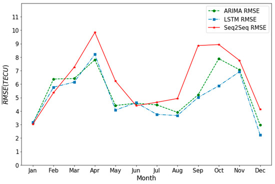
Figure 8.
The variation of the averaged RMSE in different months by three algorithms (green: ARIMA; blue: LSTM; red: Seq2Seq).
On the other hand, since the TEC data as an important parameter of the ionosphere variation has significant time-varying characteristics, the correlation coefficient between the predicted profile and the original TEC during the whole storm event can also be used to indicate whether prediction tendency is consistent or not and reflect the actual prediction effect. Figure 9 gives the correlation coefficients of three methods under different levels of geomagnetic storm events. The Seq2Seq method exhibits significant instability in the case of moderate geomagnetic storms (−100 nT ≤ Dstm ≤ −150 nT) whose correlation coefficients were broadly ranging from 0 to 0.9, and Seq2Seq’s median of correlation coefficient is 0.594 while the standard deviation value of correlation coefficient is 0.208. The LSTM and ARIMA have relatively better effects and only a small number of moderate geomagnetic storm events obtained a correlation coefficient less than 0.3, and their medians of correlation coefficient are bigger than those of Seq2Seq, 0.638 and 0.688, while they get a smaller standard deviation value of correlation coefficient, 0.175 and 0.150. Furthermore, in the case of great geomagnetic storms (Dstm ≤ −250 nT), the LSTM is significantly better than the other two methods. The correlation coefficients of most geomagnetic storm events are greater than 0.6.
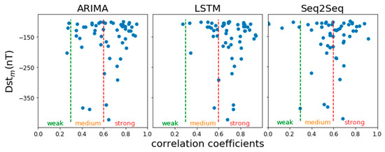
Figure 9.
The relationship between the prediction results of the three methods and the observed values under different geomagnetic storm intensities (shown by blue points). The y-axis Dstm is the same as that of Figure 5, and the x-axis is the correlation coefficient (CC) between each observation and the predicted data. The weak region (CC < 0.3) represents a weak correlation between the predicted value and the observed data. Similarly, medium (0.3 ≤ CC < 0.6) means moderately correlated, while strong (CC ≥ 0.6) is strongly correlated.
Table 3 then gives the statistical distribution of the correlation coefficient obtained by the three methods in Figure 9. The overall prediction effect of the LSTM is the best, and only 1.82% of the geomagnetic storm events fail to be predicted (weak correlation). It can be noted that the LSTM is very robust for the accurate trend prediction of the strong geomagnetic storm (more than 70%). In contrast, the ARIMA and Seq2Seq have relatively poor performance, and their prediction for the strong geomagnetic storm trends were 58.18% and 45.45%, respectively. In particular, the percentages of failure events were 5.45% and 12.73%. In summary, the LSTM method developed from a newer deep learning algorithm can achieve the best performance in predicting the trend of the ionospheric TEC variation during the storm events.

Table 3.
Statistical distribution of the correlation coefficients for three predictive methods.
4. Conclusions
During the period of a geomagnetic storm, the ionosphere often appears significantly disturbed. In such a case, the ionospheric related measurements (e.g., TEC, foF2) are significantly lower or higher than those during the quiet period, which is highly random in time and therefore is too difficult to be predicted accurately. In this paper, two deep leaning algorithms (LSTM and Seq2Seq) are used to predict the ionospheric TEC variation under different geomagnetic activity events and compared with the result from the traditional method ARIMA. Our conclusions are as follows.
- The geomagnetic storm can significantly affect the prediction performance of these three methods. During the geomagnetic quiet period, the ARIMA and Seq2Seq will have more deviation and unusual spikes under moderate and strong geomagnetic storm conditions. The LSTM can achieve the best performance.
- Based on statistical analysis of 55 geomagnetic storm events (minimum Dst ≤ −100 nT) selected from 2001 to 2016, the RMSE and the correlation coefficient of the prediction trend changes were carefully studied under different geomagnetic storm intensities. The LSTM, a deep learning algorithm, is superior to the traditional ARIMA and the Seq2Seq. The overall prediction effect of the LSTM is the best. It is very robust for accurate trend prediction of strong geomagnetic storms (more than 70%). In contrast, the ARIMA and Seq2Seq have relatively poor performance, and their predictions for the strong geomagnetic storm trends were 58.18% and 45.45%.
- The Seq2Seq method used in this paper is based on the original RNN algorithm, which is sensitive to a short-term TEC feature. Therefore, more random noise is involved and adopted by the final model during the training process. It finally results in higher randomness and error in the prediction performance. On the other hand, the LSTM can learn both features of the long-term and short-term trend of TEC in the training process. It significantly adds a hidden state, called ’cell state’, in the hidden layer of the recurrent structure. This state can make optimal decisions to keep or forget the knowledge they have learned from long-term or short-term trend variation of the ionospheric TEC data. In such a case, the LSTM can effectively provide a high level and more accurate prediction for most of the moderate and strong geomagnetic storms.
- All the algorithms show consistent seasonal dependence in the storm-time ionospheric prediction, which clearly suggests that seasonal variation is an important factor to affect the performance of prediction.
Moreover, the training data is also an important factor to affect the performance of the deep learning methods, especially in different regions. However, the ability of capturing the impact of geomagnetic storm is limited; in this research, super-geomagnetic storms are always hard to be captured, which may be due to the fact that the number of extreme storm events in our training data are too few, so that their features are hard to be learned by the deep learning models (LSTM or Seq2Seq). The prediction performance of the main phase in some super geomagnetic storms is still limited for the present three methods. In the future, the dependence of the robustness of these methods on the different spatial conditions, such as high and low latitude, will be further studied.
Author Contributions
Z.C. gave the basic idea of the paper. R.T., F.Z., and Z.C. designed the experiments and analysis tools, performed the experiments, and analyzed the data; J.-S.W., C.-M.H., and Z.W. participated in discussion and interpretation of the data. R.T. and Z.C. wrote the paper. All authors have read and agreed to the published version of the manuscript.
Funding
This research was funded by the National Natural Science Foundation of China (grant no. 41604136, 41674144, 41774195, 41974183, and 41974195).
Acknowledgments
The MIT-TEC data are obtained from MIT haystack madrigal dataset (http://madrigal.haystack.edu/madrigal/). We thank these organizations for making their data public.
Conflicts of Interest
The authors declare no conflict of interest.
References
- Zhou, M.; Ashour-Abdalla, M.; Deng, X.; Schriver, D.; El-Alaoui, M.; Pang, Y. THEMIS observation of multiple dipolarization fronts and associated wave characteristics in the near-Earth magnetotail. Geophys. Res. Lett. 2009, 36. [Google Scholar] [CrossRef]
- Tang, R.; Summers, D.; Deng, X. Effects of cold electron number density variation on whistler-mode wave growth. Ann. Geophys. 2014, 32, 889–898. [Google Scholar] [CrossRef]
- Vemareddy, P.; Mishra, W. A full study on the Sun–Earth connection of an Earth-directed CME magnetic flux rope. Astrophys. J. 2015, 814, 59. [Google Scholar] [CrossRef]
- Lowder, C.; Qiu, J.; Leamon, R.J. Coronal Holes and Open Magnetic Flux over Cycles 23 and 24. Sol. Phys. 2016, 292, 18. [Google Scholar] [CrossRef]
- Ashour-Abdalla, M.; El-Alaoui, M.; Goldstein, M.L.; Zhou, M.; Schriver, D.; Richard, R.; Walker, R.; Kivelson, M.G.; Hwang, K.-J. Observations and simulations of non-local acceleration of electrons in magnetotail magnetic reconnection events. Nat. Phys. 2011, 7, 360–365. [Google Scholar] [CrossRef]
- Zhou, M.; Pang, Y.; Deng, X.H.; Yuan, Z.; Huang, S.Y. Density cavity in magnetic reconnection diffusion region in the presence of guide field. J. Geophys. Res. Space Phys. 2011, 116. [Google Scholar] [CrossRef]
- Zhou, M.; Ashour-Abdalla, M.; Berchem, J.; Walker, R.J.; Liang, H.; El-Alaoui, M.; Goldstein, M.L.; Lindqvist, P.A.; Marklund, G.; Khotyaintsev, Y.V.; et al. Observation of high-frequency electrostatic waves in the vicinity of the reconnection ion diffusion region by the spacecraft of the Magnetospheric Multiscale (MMS) mission. Geophys. Res. Lett. 2016, 43, 4808–4815. [Google Scholar] [CrossRef]
- Zhou, M.; El Alaoui, M.; Lapenta, G.; Berchem, J.; Richard, R.L.; Schriver, D.; Walker, R. Suprathermal Electron Acceleration in a Reconnecting Magnetotail: Large-Scale Kinetic Simulation. J. Geophys. Res. Space Phys. 2018, 123, 8087–8108. [Google Scholar] [CrossRef]
- Zhou, M.; Ni, B.; Huang, S.Y.; Deng, X.; Ashour-Abdalla, M.; Nishimura, Y.; Yuan, Z.; Pang, Y.; Li, H. Observation of large-amplitude magnetosonic waves at dipolarization fronts. J. Geophys. Res. Space Phys. 2014, 119, 4335–4347. [Google Scholar] [CrossRef]
- Fuller-Rowell, T.J.; Codrescu, M.V.; Moffett, R.J.; Quegan, S. Response of the thermosphere and ionosphere to geomagnetic storms. J. Geophys. Res. Space Phys. 1994, 99, 3893. [Google Scholar] [CrossRef]
- Mannucci, A.J.; Tsurutani, B.T.; Iijima, B.A.; Komjathy, A.; Saito, A.; Gonzalez, W.D.; Guarnieri, F.L.; Kozyra, J.U.; Skoug, R. Dayside global ionospheric response to the major interplanetary events of October 29–30, 2003 “Halloween Storms”. Geophys. Res. Lett. 2005, 32. [Google Scholar] [CrossRef]
- Wang, W.; Lei, J.; Burns, A.G.; Solomon, S.C.; Wiltberger, M.; Xu, J.; Zhang, Y.; Paxton, L.; Coster, A. Ionospheric response to the initial phase of geomagnetic storms: Common features. J. Geophys. Res. Space Phys. 2010, 115. [Google Scholar] [CrossRef]
- Chen, Z.; Wang, J.-S.; Deng, Y.; Deng, Y.; Huang, C.; Li, H.M.; Wu, Z.X. Study on the relationship between the residual 27 day quasiperiodicity and ionospheric Q disturbances. J. Geophys. Res. Space Phys. 2017, 122, 2542–2550. [Google Scholar] [CrossRef]
- Prölss, G.W. Magnetic storm associated perturbations of the upper atmosphere. Sea Ice 1997, 98, 227–241. [Google Scholar]
- Mendillo, M. Storms in the ionosphere: Patterns and processes for total electron content. Rev. Geophys. 2006, 44. [Google Scholar] [CrossRef]
- Wang, J.-S.; Chen, Z.; Huang, C.-M. A method to identify aperiodic disturbances in the ionosphere. Ann. Geophys. 2014, 32, 563–569. [Google Scholar] [CrossRef][Green Version]
- Chen, Z.; Wang, J.; Huang, C.; Huang, L. A new pair of indices to describe the relationship between ionospheric disturbances and geomagnetic activity. J. Geophys. Res. Space Phys. 2014, 119. [Google Scholar] [CrossRef]
- Chen, Z.; Wang, J.-S.; Deng, Y.; Huang, C.-M. Extraction of the geomagnetic activity effect from TEC data: A comparison between the spectral whitening method and 28 day running median. J. Geophys. Res. Space Phys. 2017, 122, 3632–3639. [Google Scholar] [CrossRef]
- Buonsanto, M. Ionospheric Storms—A Review. Space Sci. Rev. 1999, 88, 563–601. [Google Scholar] [CrossRef]
- Fuller-Rowell, T.J.; Codrescu, M.C.; Wilkinson, P. Quantitative modeling of the ionospheric response to geomagnetic activity. In Annales Geophysicae; Springer: Berlin/Heidelberg, Germany, 2000; Volume 18, pp. 766–781. [Google Scholar]
- Schunk, R.; Thompson, D.C.; Sojka, J.J.; Zhu, L.; Scherliess, L. Ionospheric Weather Forecasting on the Horizon. Space Weather. 2005, 3. [Google Scholar] [CrossRef]
- Jin, S.; Jin, R.; Kutoglu, H. Positive and negative ionospheric responses to the March 2015 geomagnetic storm from BDS observations. J. Geod. 2017, 91, 613–626. [Google Scholar] [CrossRef]
- Chen, L.; Wang, S.; Fan, W.; Sun, J.; Naoi, S. Beyond human recognition: A CNN-based framework for handwritten character recognition. In Proceedings of the 2015 3rd IAPR Asian Conference on Pattern Recognition (ACPR), Kuala Lumpur, Malaysia, 3–6 November 2015; pp. 695–699. [Google Scholar]
- Brockwell, P.J.; Davis, R.A. Introduction to Time Series and Forecasting; Springer Science and Business Media LLC: Berlin/Heidelberg, Germany, 2002; Volume 2. [Google Scholar]
- Zhang, X.; Ren, X.; Wu, F.; LU, Q. Short-term TEC prediction of ionosphere based on ARIMA model. Acta Geod. Cart. Sin 2014, 2, 118–124. [Google Scholar] [CrossRef]
- LeCun, Y.; Bengio, Y.; Hinton, G. Deep learning. Nature 2015, 521, 436. [Google Scholar] [CrossRef] [PubMed]
- Xenos, T.D. Neural-network-based prediction techniques for single station modeling and regional mapping of the foF2 and M (3000) F2 ionospheric characteristics. Nonlinear Proc. Geoph. 2002, 9, 477–486. [Google Scholar] [CrossRef][Green Version]
- Oyeyemi, E.O.; McKinnell, L.A.; Poole, A.W.V. Near-real time foF2 predictions using neural networks. J. Atmos. Sol. Terr. Phys. 2006, 68, 1807–1818. [Google Scholar] [CrossRef]
- Mandrikova, O.V.; Fetisova, N.V.; Al-Kasasbeh, R.T.; Klionskiy, D.M.; Geppener, V.V.; Ilyash, M.Y. Ionospheric parameter modelling and anomaly discovery by combining the wavelet transform with autoregressive models. Ann. Geophys. 2015, 58, 550. [Google Scholar]
- Sun, W.; Xu, L.; Huang, X.; Zhang, W.; Yuan, T.; Chen, Z.; Yan, Y. Forecasting of ionospheric vertical total electron content (TEC) using LSTM networks. In Proceedings of the 2017 International Conference on Machine Learning and Cybernetics (ICMLC), Ningbo, China, 9–12 July 2017; Volume 2, pp. 340–344. [Google Scholar]
- Cherrier, N.; Castaings, T.; Boulch, A. Deep Sequence-to-Sequence Neural Networks for Ionospheric Activity Map Prediction; Springer Science and Business Media LLC: Berlin/Heidelberg, Germany, 2017; Volume 10638, pp. 545–555. [Google Scholar]
- Gruet, M.A.; Chandorkar, M.; Sicard, A.; Camporeale, E. Multiple-Hour-Ahead Forecast of the Dst Index Using a Combination of Long Short-Term Memory Neural Network and Gaussian Process. Space Weather. 2018, 16, 1882–1896. [Google Scholar] [CrossRef]
- Tan, Y.; Hu, Q.; Wang, Z.; Zhong, Q. Geomagnetic Index Kp Forecasting With LSTM. Space Weather. 2018, 16, 406–416. [Google Scholar] [CrossRef]
- Chen, Z.; Jin, M.; Deng, Y.; Wang, J.-S.; Huang, H.; Deng, X.; Huang, C. Improvement of a Deep Learning Algorithm for Total Electron Content Maps: Image Completion. J. Geophys. Res. Space Phys. 2019, 124, 790–800. [Google Scholar] [CrossRef]
- Geurts, M.; Box, G.E.P.; Jenkins, G.M. Time Series Analysis: Forecasting and Control. J. Mark. Res. 1977, 14, 269. [Google Scholar] [CrossRef]
- Yi, H.; Jung, H.; Bae, S. Deep Neural Networks for traffic flow prediction. In Proceedings of the 2017 IEEE International Conference on Big Data and Smart Computing (BigComp), Jeju, South Korea, 13–16 February 2017; pp. 328–331. [Google Scholar]
- Wang, J.; Tang, J.; Xu, Z.; Wang, Y.; Xue, G.; Zhang, X.; Yang, D. Spatiotemporal modeling and prediction in cellular networks: A big data enabled deep learning approach. In Proceedings of the IEEE INFOCOM 2017—IEEE Conference on Computer Communications, Atlanta, GA, USA, 1–4 May 2017; pp. 1–9. [Google Scholar]
- Zhang, Q.; Yang, L.T.; Chen, Z.; Li, P. A survey on deep learning for big data. Inf. Fusion 2018, 42, 146–157. [Google Scholar] [CrossRef]
- Dorffner, G. Neural networks for time series processing. Neural Netw. World 1996, 6, 447–468. [Google Scholar]
- Connor, J.T.; Martin, R.D.; Atlas, L.E. Recurrent neural networks and robust time series prediction. IEEE Trans. Neural Networks 1994, 5, 240–254. [Google Scholar] [CrossRef] [PubMed]
- Bengio, Y.; Simard, P.; Frasconi, P. Learning long-term dependencies with gradient descent is difficult. IEEE Trans. Neural Networks 1994, 5, 157–166. [Google Scholar] [CrossRef] [PubMed]
- Hochreiter, S. Recurrent neural net learning and vanishing gradient. Int. J. Uncertainity Fuzziness Knowl. Based Syst. 1998, 6, 107–116. [Google Scholar] [CrossRef]
- Hochreiter, S.; Schmidhuber, J. Long Short-Term Memory. Neural Comput. 1997, 9, 1735–1780. [Google Scholar] [CrossRef]
- Sutskever, I.; Vinyals, O.; Le, Q.V. Sequence to sequence learning with neural networks. In Advances in Neural Information Processing Systems; Curran Associates: Dutchess, NY, USA, 2014; pp. 3104–3112. [Google Scholar]
- Cho, K.; Van Merrienboer, B.; Gulcehre, C.; Bahdanau, D.; Bougares, F.; Schwenk, H.; Bengio, Y. Learning Phrase Representations using RNN Encoder–Decoder for Statistical Machine Translation. In Proceedings of the 2014 Conference on Empirical Methods in Natural Language Processing (EMNLP), Doha, Qatar, 25–29 October 2014; pp. 1724–1734. [Google Scholar]
- Hernández-Pajares, M. IGS ionosphere WG status report: Performance of IGS ionosphere TEC maps-position paper. In Proceedings of the 2004 IGS Workshop, Presented at IGS Technical Meeting, Bern, Switzerland, 2004. [Google Scholar]
- Rideout, W.; Coster, A. Automated GPS processing for global total electron content data. GPS Solutions 2006, 10, 219–228. [Google Scholar] [CrossRef]
- Madrigal CEDAR Database. Available online: http://cedar.openmadrigal.org/ftp/ (accessed on 21 March 2020).
- Gonzalez, W.D.; Joselyn, J.A.; Kamide, Y.; Kroehl, H.W.; Rostoker, G.; Tsurutani, B.T.; Vasyliunas, V.M. What is a geomagnetic storm? J. Geophys. Res. Space Phys. 1994, 99, 5771–5792. [Google Scholar] [CrossRef]
© 2020 by the authors. Licensee MDPI, Basel, Switzerland. This article is an open access article distributed under the terms and conditions of the Creative Commons Attribution (CC BY) license (http://creativecommons.org/licenses/by/4.0/).