Abstract
For coastal engineering studies and the efficient design of ports and harbors, reliable information concerning wave conditions in nearshore and coastal sites is needed. In the absence of long-term wave data at the site of interest, this becomes possible by using offshore data, which are usually available in the nearby geographical area, in addition to bathymetric and coastline information concerning the nearshore area and the local site. The latter are used in conjunction with a suitable wave model, which calculates the offshore-to-nearshore transformation of wave conditions and incorporates the relevant shallow-water phenomena. In the present work, the above methodology is applied to calculate the nearshore wave conditions in the Bay of Sitia, Crete, by applying the Simulating WAves Nearshore (SWAN) model. The interesting feature of the Bay of Sitia is its vulnerability due to strong erosion, which downgrades the touristic value of the beach. Furthermore, nearshore wave data offer valuable information concerning further coastal and port engineering studies. In this context, results from directional extreme value analysis of the nearshore wave conditions in the Sitia Bay are derived and used to investigate resonances in the enclosed marina of the Sitia port, by taking into account the depth variations inside the basin. To this end, a novel method was developed based on the modified mild-slope equation, in conjunction with the Finite Element Model, for the solution of the nonlinear eigenvalue problem.
1. Introduction
In a wide range of applications taking place in the marine environment, including the analysis of marine structures, the study of coastal processes, as well as coastal and port engineering studies, information concerning the wave climate in nearshore and coastal areas is derived by offshore-to-nearshore transformation of wave conditions; e.g., [1,2]. This is because local buoy measurements are usually not available at the site of interest, and reliable information from satellite measured data and operational wave models with global coverage and long duration are available at some distance from the coast [3].
In the present work, results from the study of the wave climate in the bay of Sitia, Crete are presented, as obtained by offshore-to-nearshore transformation of wave conditions, using the SWAN wave model [4,5]. The particular site, shown in Figure 1, has been studied in previous works [3] in the context of erosion phenomena observed at a nearby beach. Additionally, the touristic activities in the wider area have recently become more intensive, rendering confronting, prediction, and management of erosion to be more imperative. More specifically, aerial photographs, between 1945 and 2014, indicate that the coastline has retreated by 45 m (the maximum value) [6], while aerial images from Google Earth show that 7 m was the maximum loss during the period 2002–2015; see in [7] (Figure 1). The observed erosion trends could be partially attributed to the extension of the Sitia port facilities, including the extension of protruding breakwaters that has been completed over a decade ago. The justification for this interaction lays on the well-known fact that such structures could potentially modify the wave and flow conditions in the adjacent coastal zone, and as a result, sandy beaches often erode; see, e.g., [8,9]. It should be mentioned, however, that sediment transport leading to beach erosion is a long-term integrator of many processes and wave forcing could constitute only one part and its importance can be assessed only with a holistic approach.
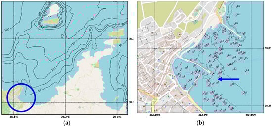
Figure 1.
(a) The nearshore area of Sitia in the northeastern part of the Crete island. (b) The port of Sitia including the enclosed touristic marina (map tiles: © OpenStreetMap contributors 2019; https://www.openstreetmap.org/copyright, bathymetric data: GEBCO Compilation Group (2019) GEBCO 2019 Grid).
Furthermore, the modification of the nearshore and onshore wave conditions is a factor that could also have important effects on harbor resonances, as is the case with the enclosed touristic marina of the Sitia port area, shown in Figure 1b. In fact, although the prevailing wave conditions in the considered area are waves from northern and northeastern directions, there is a small population of waves from the eastern directions (indicated by an arrow in Figure 1b) that could lead to the excitation of strong resonance phenomena that lead in turn, to flood events.
Focusing on the port resonant phenomena in the frequency band of wind waves, an important task of the present work was the identification of the wave conditions in the studied nearshore area from data derived from the directional extreme value analysis. Data on wave conditions were obtained by a transformation of offshore wave data. These provide the required information for investigation of possible matching with the marina resonant frequencies. A novel aspect of this work is that the harbor resonances were calculated by means of the Modified Mild Slope wave model, and were formulated in the frequency domain with variable parameters, in order to account for seabed variability. Since the model coefficients were dependent on frequency, the above model led to the formulation of a nonlinear eigenvalue boundary problem, which was treated by a finite element method (FEM) in conjunction with a Galerkin scheme. The present analysis was restricted to incident wave generated from wind and did not account for infragravity excitation or other mechanisms that could excite long-period resonances.
The paper is organized as follows. In Section 2, the bathymetric and coastal data of the extended area were initially presented and discussed. Next, these were employed, in conjunction with the SWAN model, to derive and compare the wave climatology, both offshore and nearshore. Additionally, in the same section, the data sources for the offshore wave conditions were discussed. Next, in Section 3, the offshore and the derived nearshore wave statistics were presented and discussed, including the bivariate wave height, period data, and marginal wave directions. Three nearshore points were considered at depths 55 m, 30 m, and 17 m, where the last point represented conditions outside the Sitia port area. Subsequently, in Section 4, the extreme value analysis of the wave data from all wave directions was presented, from which the most severe conditions affecting the wave field inside the port were found. In the last part of this work (Section 5), a novel FEM model of the modified mild-slope equation (described in [10]) was extended to calculate the resonances in the harbor area, including the eigenfrequencies and the corresponding eigenmodes, taking into account depth variations in the enclosed domain. The results enabled the correlation with wave excitation from specific directions and the derivation of useful conclusions and suggestions concerning the studied area.
2. Geographical and Offshore Wave Data in the Studied Area
The nearshore area of Sitia is located in the northeastern part of the Prefecture of Lassithi, Crete, on the west side of the homonymous gulf; see Figure 2. The southern part of the coastal area is a 2-km-long beach with a variable width of a maximum value around 35 m, and exhibited a typical U-shape in the NW-SE orientation. Due to the shape and orientation of the beach, the wave action is confined to the north and northeastern directions, which is the primary factor for the movement of sediments. At the western part of the beach, there is a homonymous port that can accommodate both small fishing vessels and larger merchant and passenger vessels. The town of Sitia has become a tourist attraction, mainly during the summer period, while tourist infrastructures (e.g., hotels, restaurants), and in general human activities, place pressure on the coastal environment. The smaller enclosed harbor constitutes a protected basin that also serves as a touristic marina.
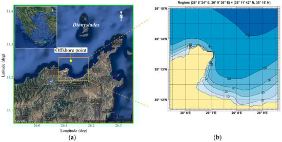
Figure 2.
(a) Aerial map of the Sitia gulf from Google Earth, showing the location of the ERA-Interim offshore grid point; and (b) Bathymetry and coastline data used for the offshore-to-nearshore transformation of wave data.
2.1. Offshore Wave and Wind Data
Various sources of offshore wave and wind data are available covering the sea area of interest. The most complete databases come from application of wave models that are operationally run at meteorological and oceanographic centers and from dedicated long-term hindcasts. Moreover, satellite data with good spatial coverage of offshore waters around the world are available. Concerning wave model data, a limiting factor is the accuracy of input wind fields, to which the model results are sensitive. In-situ data from buoy wave measurement networks are very accurate; however, these are relatively few and spatially very sparse. The offshore data used in the present study are described below.
Regarding the wave climatology of the study area, the analysis relies on a long-term time series, between 01/1979 and 12/2014, at the offshore point (see Figure 2) with geographical coordinates (35.25° Ν–26.125° Ε) and a water depth of 107 m, derived from the European Centre for Medium-Range Weather Forecasts (ECMWF) Re-Analysis Interim (ERA-Interim) database [11]. The relevant information includes significant wave height , energy wave period , and mean wave direction (measured clockwise from north), with a 6-h temporal resolution. The dataset also contains wind speed () and mean wind direction. The basic statistical measures concerning wave characteristics (i.e., , , and ) at the offshore point, including sample size (N), mean value (m), standard deviation (s), minimum (min) and maximum (max) values, skewness (Sk), and kurtosis (Ku) coefficients, are presented in Table 1. For a linear variable, say , skewness and kurtosis are defined as and , respectively. For a directional variable, say , circular skewness and circular kurtosis are estimated by and , respectively.

Table 1.
Statistics of wave parameters from offshore time-series between 01/1979 and 12/2014.
On average, the wave intensity was characterized as low, with mean values m, s and deg. The most intense waves occurred with m, during a two-day storm. The skewness coefficient of offshore wave height data indicated that the data were left-skewed, while the value of kurtosis indicated a sharp peak of the distribution. The offshore waves were concentrated to northern–northwestern directions, while a secondary peak was also observed from the western directions. The marginal distributions of offshore wave data and the bivariate distribution are presented in Figure 3, as obtained using standard parametric and non-parametric models; for more details, see [12].
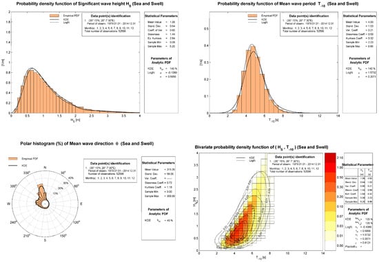
Figure 3.
Offshore wave data at a Sitia offshore point (35.35° N, 26.125° E); depth 107 m.
2.2. Bathymetry and Coastline Data
For the present study, the bathymetric data used in the SWAN wave model for the offshore-to-nearshore transformation of wave conditions in the extended geographical area were created by the combination of the European Marine Observation and Data Network (EMODnet) Bathymetry Consortium and data from the maps of the Greek Navy Hydrographic Service for areas near the coast. EMODnet Digital Bathymetry (DTM 2016) was based upon more than 7700 bathymetric data sets from various countries near the European Seas and it is provided on a grid resolution of 1/8 by 1/8 arc minute of longitude and latitude [13]. The database used for the coastline was the Global, Self-consistent, Hierarchical, High-resolution Shoreline Database (GMT–GSHHS) provided under the GNU Lesser General Public License; see [14].
3. Offshore-to-Nearshore Wave Transformation
Offshore-to-nearshore sea-state transformation techniques enable us to derive wave information in the domain from offshore wave data. In the present work, the methodology described in [15] was used. Results were stored for the three indicated nearshore target points shown in Figure 4, located at depths 58 m, 29 m and 17 m, and consecutively numbered. The location of the offshore point was displayed by a red dot.
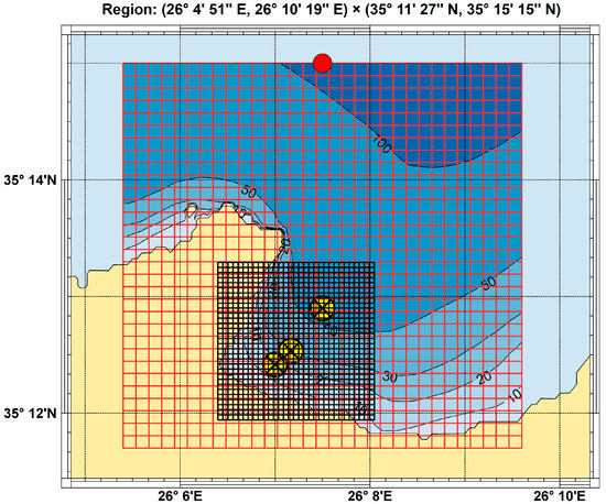
Figure 4.
Bathymetric data in the area of interest and the set-up of the SWAN model for calculating the offshore-to-nearshore wave transformation. Results are stored for the three indicated nearshore target points. The offshore point is shown by a red dot.
The offshore time-series of wave data (significant wave height, mean energy period and mean wave direction) were used as uniform boundary conditions applied to the northern offshore boundary of the considered domain, for calculating the wave propagation in the region, using the spectral wave model SWAN [4,5]. Additional information concerning wind speed and mean wind direction that was available from the offshore data, was also used as a uniform forcing, all over the modelled region. A uniform grid (of average size ~ 450 m) covering the region was used for the numerical simulation, as shown in Figure 4. In addition, a nested grid with a much finer resolution (mean gridsize ~150 m) was used around the three nearshore target points, as depicted in Figure 4. After the simulation covering the 36-year period of offshore wave data, the time series of directional wave spectra were derived for all three nearshore target points, from which the spectral parameters were calculated. More details concerning the offshore-to-nearshore wave transformation by the above model, including spatial plots of wave height and direction are presented in Appendix A.
Wave Climatology in the Sitia Gulf Area
The offshore and nearshore wave univariate distributions concerning the significant wave height (), mean energy wave period (), mean wave direction (), and the bivariate variables distribution are presented comparatively in Figure 3, Figure 5, Figure 6 and Figure 7, respectively. In addition to the histograms (empirical distribution), analytical probability models fitting the data using standard parametric and non-parametric univariate and bivariate models are also shown; see [8]. In particular, the results shown in Figure 7 represent the wave conditions near the mouth of the Sitia port area.
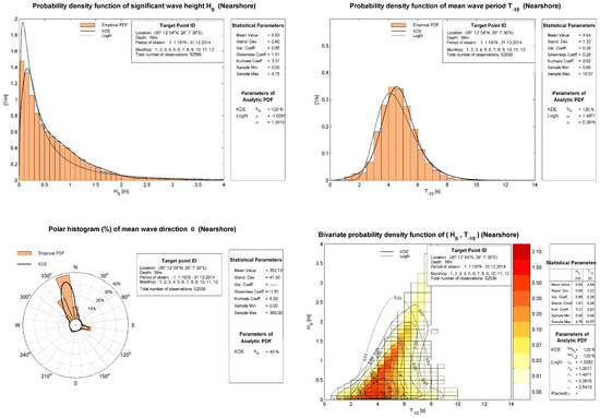
Figure 5.
Wave data in the Sitia Bay area at nearshore point 1, at a depth of 58 m.

Figure 6.
Wave data in the Sitia Bay area at nearshore point 2, at a depth of 29 m.

Figure 7.
Wave data in the Sitia Bay area at nearshore point 3, at a depth of 17 m.
It can be observed in Figure 3 that the prevailing offshore waves in the region were from north-northwestern and western directions, while at the nearshore area, the wave conditions were modified as follows:
- (i)
- At nearshore point 1, the wave directions concentrated around the north-northwestern directions, due to the effects of refraction, diffraction, and sheltering by the Sitia peninsula. However, a secondary population of waves from the eastern directions also appeared, which were mainly attributed to wind from eastern directions.
- (ii)
- Moving closer to the shore, the effects of refraction due to bathymetric variations become more significant. These are clearly depicted in Figure 6, Figure 7 (which presents the wave statistics based on the wave data calculated at nearshore points 2 and 3, respectively), and, in particular, in the corresponding wave-rose diagrams. As a result, there was a concentration of the majority of the waves in the northeastern sector. Moreover, a secondary peak of waves from the eastern directions appeared.
- (iii)
- As we move closer to the entrance of the port area of Sitia, at nearshore point 3, a secondary peak of waves from the eastern directions was present.
The mean values of the calculated wave parameters concerning the significant wave height , the mean energy period , the primary peak, and secondary peak of the distribution of wave directions are comparatively listed in Table 2. Although the wave conditions in the nearshore area (as derived from the above analysis) were significantly more mild and the mean wave heights were reduced to 33% of the corresponding offshore values, the results from the directional extreme value analysis (which is presented in more detail in the next section) indicate that incidents with increased energy from the east were not rare. The latter could excite resonance in the enclosed protected port and were potentially responsible for the flooding events that were observed in the past years.
Table 2.
Basic statistics of the wave parameters at offshore and nearshore points.
4. Directional Extreme Wave Data Analysis at Offshore and Nearshore Points
In order to ensure that offshore and coastal structures are reliable both in terms of structure and economic viability, it is of paramount importance to accurately estimate the behavior of the extreme values of the involved environmental variables during the design process and risk assessment. The literature on extreme value modeling of wave parameters is rich; e.g., [16,17,18]. Typical wave parameters that are analyzed in the context of extreme value analysis through statistical approaches are wave height and wave period, which are mainly obtained through long-term (of the order of 30 years or more) hindcast databases and measurements with constant statistical properties in time. However, there are some factors that affect wave regimes and violate the assumption of stationarity since spatial, temporal or directional variations might take place in the long-term study of a phenomenon. The dependence of direction on the variability of a specific parameter is also evident; a typical example is the generation of higher waves at particular directional sectors, compared to others at an offshore location. This is clearly also the case of the present study since refraction and diffraction in conjunction with wind forcing produce an excitation at the entrance of the enclosed basin of the Sitia marina.
In order to incorporate the directional characteristics in the extreme value model, different approaches have been examined. After selecting the appropriate values of significant wave height above a certain threshold for the extreme value analysis, they are binned into sectors, either arbitrarily based on the directionality of the data or fixed, usually into eight sectors, assuming homogeneity within the sectors, in both cases. Then, for each directional sector, extremal analysis is performed to estimate the design values for a given return period. Another approach is to model the extreme values as a function of all directions. For the description of the latter model, it is expected that the extreme value parameters vary smoothly with direction. In the next part of this section, the directional extreme value model will be described and comparison of the results between the offshore and all nearshore points will be presented and discussed.
4.1. Directional Model and Parameter Estimation
Let us consider a sample with values of significant wave height along with the corresponding values for the wave direction . Assuming that the Generalized Pareto (GP) distribution describes the extreme observations above a threshold , which is considered to be independent of the directional variable, the cumulative distribution function is given by
where and both unknown parameters (i.e., and ) are expressed as functions of .
In the context of estimating the unknown parameters, as noted by [19], it is expected that they vary smoothly with direction; thus, a Fourier series expansion is used for the description of this (angular) dependence, which assures a periodic behavior of the estimates in terms of the direction. In this context, the general form of the Fourier series is for the unknown parameters and
respectively, where denotes the order of the Fourier model, and , is the cosine and sine function, respectively. It is evident that the more complex the directional dependence that characterize the data sample, the higher is the model order [20].
The unknown parameters and , and are estimated by applying maximum likelihood estimation. The likelihood of the corresponding data sample , where is the number of observation exceeding the threshold , is given by
and the negative log-likelihood
The maximum likelihood estimates are determined by using the numerical optimization technique of Nelder–Mead [21], as is employed by the ‘extRemes’ package, version 2.0–10, in R [22]. This software facilitates the fitting of extreme value distributions with the covariates in the parameters.
The a priori selection of a suitable threshold implies the existence of an additional unknown parameter for GP distribution, which might affect the validity of the estimates and is still an open issue with no established approach. This selection is a trade-off between bias and variance. A low threshold would result in large bias and low variance, leading to incorrect results for the obtained estimates since less representative extreme data are taken into account, whereas a high threshold would result in a small bias and large variance, leading to unreliable results, due to the smaller sample size.
A plethora of statistical techniques has been proposed for the determination of the appropriate threshold; see [23] for more details. In this study, the 90th percentile of the data has been used for the selection of the extreme values of .
All examined locations were fitted with the first-order Fourier model, which seemed to be sufficient for the description of directional dependence. Indicatively, for the offshore point, the values of the estimated parameters are provided in Table 3, along with the corresponding confidence intervals by applying the percentile bootstrap method.
Table 3.
Estimates and confidence intervals for the offshore point.
In the left column of Figure 8, the functional forms of the Fourier models are presented for both parameters, with regards to offshore point and nearshore points 2 and 3. In addition, the estimates obtained from the data of successive directional sectors of width 45° are presented. Directional sectors with a sample size less than 20 were considered unreliable for fitting the GP distribution; hence, they were excluded from the standard directional analysis. As was already mentioned, nearshore points 2 and 3 were dominated by north and northeastern wave directions, due to the surrounding topography; thus, only three-directional sectors had sufficient amount of data to proceed with the statistical analysis.
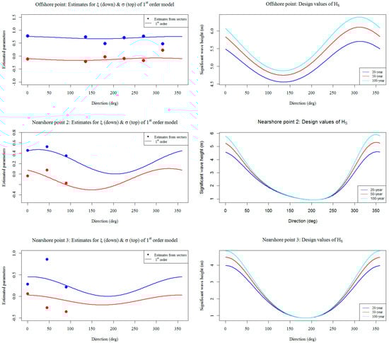
Figure 8.
Results of directional extreme analysis at offshore point and nearshore points 2 and 3.
4.2. Design Values
After obtaining the estimated parameters, the return level (that is exceeded on average once in years) by direction was obtained by
where is the observation years.
In the right column of Figure 8, the 20-, 50- and 100-year design values of are presented in terms of wave direction. The offshore point exhibited the highest extreme values of at , which was close to . With regards to the nearshore point 3, the significant wave height design values showed increased waves from the northern directions up to 4.8 m (for the 100-year period), and up to 2 m for the eastern directions. A similar behavior was presented for nearshore point 2.
In Figure 9a, the bivariate histogram of peak wave periods and significant wave heights is provided, for directions in the sector at nearshore point 3, with regards to the entire time-series. For the more energetic sea states characterized by m, shown by using a dashed box in Figure 9a, the mean energy periods were s, and the corresponding values of the peak period were s. The latter conditions were studied in connection with the possible excitation of resonance in the enclosed protected port, in the next section.

Figure 9.
(a) Conditional distribution of wave periods and wave heights at nearshore point 3 in the eastern wave sector 75°105°, and; (b) corresponding distribution of wave periods at the same point, as calculated by offshore-to-nearshore transformation.
5. Study of Port Resonances in the Enclosed Small Port of Sitia, Crete
An aerial photo of the site is shown in Figure 10 and photos of the parts of enclosed small port and the marina are presented in Figure 11, respectively.

Figure 10.
Aerial photo of the Sitia port area.
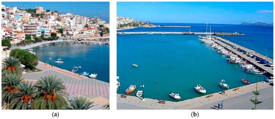
Figure 11.
(a) The western part, and (b) the eastern part of the enclosed port/marina.
The detailed bathymetry of the Sitia port and the coastal area is based on data from local nautical maps (scale 1:5000) and subsequently processed to derive a local digital bathymetric model, as presented in Figure 12a, with the location of the nearshore point 3 indicated by a circle, where wave data are available from offshore-to-nearshore transformation, as described in previous sections. In addition, the detailed bathymetry inside the enclosed small marina area is shown in Figure 12b.
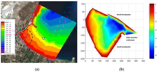
Figure 12.
(a) Bathymetry (depth in meters) of the Sitia port and the nearshore/coastal area. The location of nearshore point 3, where the wave data were calculated by using the offshore-to-nearshore wave transformation was indicated by using a circle; and (b) detailed bathymetry and solid-wall boundaries in the enclosed port, including the small marina. Horizontal distances are in meters.
Standard methods to treat the problems of basin oscillations in closed or semi-closed domains are based on variants of the Helmholtz equation; e.g., [24,25]. In the case of relatively small water depths, and with regards to the first larger eigenperiods, shallow-water models were also applicable. However, for moderate wave periods, as in the present case of port resonances excited by the nearshore waves in the variable bottom topography, the mild-slope equations were preferred, since they took into account the dispersion effects.
A standard model describing the propagating-refracted-diffracted wavefield over a general bathymetry domain, which is characterized by slowly varying depth , is the modified mild-slope (MMS) equation:
where is the domain; see [26,27]. In the above equation, is the phase velocity and is the corresponding group velocity, where the angular frequency of the monochromatic incident wave is denoted by and the local wavenumber by . The latter, at specific frequency , is obtained from the water-wave dispersion relation,
formulated at the local depth, with being the acceleration of gravity. Moreover, the function involves terms associated with bottom slope and curvature and can be found in [26] (Equation (34)); see also [27]. The mild-slope model was successfully applied to similar problems of water-wave propagation, and diffraction in the presence of bathymetric inhomogeneities and structures in general bathymetry regions by [10], using a parameter-free perfectly matched layer (PML)-FEM formulation. Notably, the MMS Equation (6) could be extended to account for dissipation mechanisms, such as seabed friction and wave breaking, by including an appropriate imaginary part in the wavenumber [26,28]. However, this was outside the scope of the present work. Moreover, in order to account for nonlinear transformations taking place in the surf zone, such as, breaking, run-up, and wave–wave interaction, more advanced Boussinesq-type models [29] or fully dispersive models need to be considered [30].
For studying the port resonances in the enclosed basin, Equation (6) was supplemented by appropriate boundary conditions along the boundary . The latter consists of the homogeneous Neumann condition , along the solid walls and homogeneous Dirichlet condition along the marina entrance; see Figure 10b. The latter are considered more appropriate for the studied problem; see [24,31,32,33].
In the present work, the eigenvalue problem formulated by means of the MMS model was considered for the study of port eigenfrequencies. A major difficulty arose from the fact that the coefficients of Equation (6) were dependent on the local depth and frequency, which introduced nonlinearity. In order to tackle such complexity and solve the non-linear eigenvalue problem, a viable numerical strategy was to employ a linear solution calculated for the domain of interest, assuming constant depth, along with a Galerkin scheme that was applied to calculate the port eigenfrequencies, using the MMS model over the realistic bathymetry. Thus, the linear Laplace eigenvalue problem was initially solved in the domain by means of low-order FEM, employing linear triangular elements. The eigenvalues and eigenmodes were calculated in the enclosed port domain satisfying the following boundary conditions on the solid walls and the port entrance, respectively,
For illustration purposes, an intermediate mesh of triangular elements, which was used to derive the Laplace eigenvalues and eigenmodes, is shown in Figure 13. The first Laplace eigenvalues and corresponding eigenfrequencies in the Sitia small harbor, calculated for the mean constant depth m are listed in Table 4. Additionally, the first four Laplace eigenmodes in the Sitia enclosed port as calculated by the present FEM model are plotted in Figure 14.
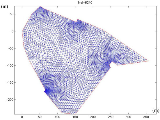
Figure 13.
Intermediate finite element method (FEM) mesh in the enclosed Sitia port (no. of elements was 6240). Horizontal distances are in meters.
Table 4.
First Laplace eigenvalues and corresponding eigenfrequencies in the Sitia small harbor domain as calculated for the mean constant depth m.

Figure 14.
Calculated (a) first; (b) second; (c) third; (d) fourth eigenmode in the Sitia enclosed port area. Horizontal distances are in meters.
Next, by exploiting the basic properties of the calculated eigensystem (8), the solution of the nonlinear eigenvalue problem was searched in the following form
where are coefficients and the number of the retained terms in the expansion Equation (9) is sufficiently large. Using the above representation in the MMS Equation (6), the latter was finally put in the form,
where
Subsequently, Equation (10) was projected on the basis and the following homogeneous algebraic system was derived
where . The matrix coefficient of the above system is
and the non-trivial solutions of Equation (12) are obtained by requiring the determinant to be zero
The roots of the above equation, with respect to the frequency ω, were calculated by a direct search method, which provided the numerical solution of the considered nonlinear eigenvalue problem.
In the scope of the present work, the analysis focused on the range of periods that correspond to the low-frequency band of wind-generated waves, obtained from the previous incident wave data analysis. The calculated MMS eigenperiods in the Sitia enclosed port, in the range , as obtained from the MMS model using the FEM–Galerkin scheme with Nelem = 24960, are shown in Figure 15, using open circles. The bars in the figure indicate the peak periods obtained from the analysis of wave data at nearshore point 3 in front of the entrance of the Sitia port, corresponding to the energetic sea states from the eastern directions, which could excite port resonances. The closest MMS eigenperiods of the enclosed port obtained from the solution of Equation (14) were {9.92 s, 9.50 s, 8.66 s, 8.49 s, 8.34 s}; shown in Figure 15, using rectangles. The corresponding calculated eigenmodes in the port area are plotted in Figure 16. It was noted, however, that the wave periods calculated from the wave transformation were dependent on frequency discretization of the models, and the matching should have been performed using a small bandwidth permitting overlapping with the identified eigenperiods.
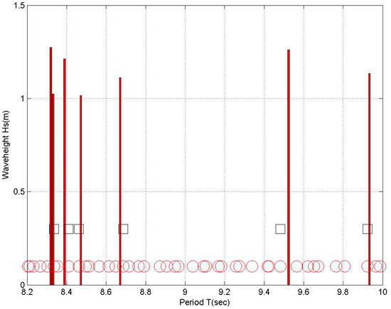
Figure 15.
Calculated modified mild-slope (MMS) eigenperiods in the Sitia enclosed port in the range , denoted by open circles. The bars indicate peak periods obtained from the analysis of wave data at nearshore point 3 in front of the entrance of the Sitia port, corresponding to the energetic sea states from east, which could excite port resonances. The closest eigenperiods of the enclosed port were {9.92 s, 9.50 s, 8.66 s, 8.49 s, 8.34 s}; denoted by rectangles.
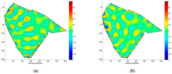

Figure 16.
The calculated eigenmodes corresponding to the eigenperiods (a) 9.92 s; (b) 9.48 s; (c) 8.68 s; (d) 8.46 s; (e) 8.33 s; (f) 8.30 s in the enclosed port, as obtained from the MMS model, using FEM with Nelem = 24,960. Horizontal distances are in meters.
The findings suggest that the incoming eastern waves through the open entrance were likely to excite port resonances. The results depicted in Figure 16 showed that resonant matching could potentially lead to flooding events in the west port wall (Figure 16a,b,f), posing a threat to the nearby hospitality infrastructure, as well as degradation of the southern pier/marina (Figure 16c,e). Both events would have a detrimental effect on the touristic value of the area; c.f. Figure 11a and b, respectively.
Except for direct forcing by wind waves, resonances in and near harbors could be due to a number of factors, as indirect forcing due to wind–wave interactions, and other long-period basin forcing and tides. Notably, the present analysis was restricted to incident wind generated waves, neglecting infragravity wave excitation and their generation mechanisms. Infragravity wave effects and their potential role to harbor resonances are documented in the literature [34,35,36,37]. The nonlinear shoaling, wave–wave interactions, and wind forcing were not addressed in the scope of the present work but they suggest interesting future extensions [38]. Finally, tidal effects in the extended geographical area of the Southern Aegean Sea and Cretan Sea were negligible; see, [39].
6. Conclusions
In the present work, the identification of wave directions from a directional extreme value model that could result in intense resonance phenomena inside the port of Sitia was examined. After transforming the available offshore wave conditions to the nearshore in the Bay of Sitia by means of the SWAN model, the obtained wave information was used for the estimation of extreme wave heights as a function of direction. Given the sets of wave heights and directions at one offshore and three nearshore locations, it was assumed that the extreme wave heights could be described by applying a Generalized Pareto distribution, with its parameters varying smoothly with direction. Design values of wave heights that also varied with direction were presented for all examined locations. The obtained results for the nearshore point at the entrance of the port (i.e., nearshore point 3) revealed that apart from the prevailing northern directions, the eastern waves could produce relatively high sea states. Then, the port resonances were investigated, taking into account the variable bathymetry of the enclosed basin, which corresponded to the principal frequency of the wave excitation in the eastern directions. The modified mild-slope equation was implemented for the description of combined refraction–diffraction effects, from which the eigenperiods were calculated by means of an FEM-Galerkin scheme. The results from the resonance analysis indicated that the western wall of the port could be affected by flood events from waves coming from the eastern sector.
Ports are vulnerable to the changes in the wave regime with the extreme events causing interruptions to port operations and in some cases even causing disruptions regarding connectivity with the neighboring infrastructure. The presented methodology provides a valuable tool for a detailed estimates of extreme wave heights and for assessing the effectiveness of common countermeasures, such as partial dredging and the installation of barriers that would alter the bathymetry within the port basin. The present analysis was restricted to incident wave generated from wind and did not account for other mechanisms of excitation, especially in the low-frequency band, which could be important. Interesting future extensions of the present work concern the treatment of infragravity wave excitation, along with other mechanisms that could excite long-period port resonances, along with the collection of required data, which were presently not available.
Author Contributions
The main draft of the text was handled by F.K. and K.B. Numerical simulations concerning wave transformation were carried out by T.G. and those concerning port resonances were carried out by A.K. and K.B. All authors have read and agreed to the published version of the manuscript.
Funding
This research received no external funding.
Conflicts of Interest
The authors declare no conflict of interest.
Appendix A. Offshore-to-Nearshore (OtN) Wave Transformation Technique
Offshore wave conditions, represented by appropriate spectral parameters (significant wave height, mean wave period, and mean wave direction), were considered to be known, all along the seaward boundary from which the directional spectrum was reconstructed, using the JONSWAP frequency spectrum, in conjunction with a hyperbolic-cosine spreading function [34]
where is the linear frequency and ω is the angular frequency, is the peak frequency estimated as , g = 9.81 m/s2 is the acceleration due to gravity, the parameter is defined by means of the formula,
and the parameter and the function are given by
The spreading function is defined by
where
The offshore wave conditions represent the main forcing of the examined system, and are continuously distributed all along the seaward boundary; for more details see [15] (Figure 1). Given the offshore boundary conditions, the phase-averaged model SWAN [4,5] was applied to calculate the wave conditions inside the computational domain, with a sufficient spatial resolution. The basic equation used in the SWAN model was the radiative transfer equation expressing action balance
in which denoted the wave action density , expressed as a function of frequency (, where k is the wavenumber modulus, g is the gravitational acceleration and is the water depth), and the wave direction . In Equation (A6), are the propagation velocity components in the physical and the Fourier-parameter spaces, respectively. The left-hand-side term of Equation (A1) represents, respectively, the local rate of change of action density in time, the propagation of action in and geographical directions, the frequency shifting due to depth variation and currents, and the depth- and current-induced refraction. Thus, the above formulation uses linear wave theory for wave propagation and accounts for diffraction effects. The forcing term is the energy source term. This term is decomposed to a number of separate source terms, as follows:
where represents the effects of generation of wave energy by wind, is the dissipation of wave energy due to white-capping (deep-water wave breaking), wave-bottom interactions, and depth-induced wave breaking in very shallow water, and represents the wave energy transfer, due to conservative nonlinear four- and three-wave interactions. Furthermore, wind generation was described in SWAN by the sum of linear and exponential growth terms [15]. The dissipation term was composed by the contributions of white-capping, bottom friction, and depth-induced breaking. With regards to the non-linear interactions, the computation of quadruplet wave–wave interactions was carried out using the discrete interaction approximation (DIA) and for triad wave–wave interactions, the Lumped Triad Approximation (LTA) was used; see [40]. The numerical integration of the action balance Equations (A6) and (A7) was implemented in SWAN, using the finite difference schemes in all five dimensions (time, geographic space, and Fourier space). In the geographical space, the discrete scheme was based on a first order upwind difference scheme. In the Fourier space, a mixed upwind/central difference scheme was used.
The OtN wave transformation model was applied to the cases characterized by bathymetry variations and its predictions were compared against calculations from more accurate phase-resolving models and experimental data [41], showing good agreement. The numerical parameters used in the present model, which were found to be sufficient for convergence of the results, were: (i) discretization of physical-space grid size for both the global and local nested grid 31 × 31 (see Figure 4), (ii) discretization of frequency-direction space 18x24, with the lowest value of the discrete frequency set at 0.6fp and the highest value at 3fp. Furthermore, the rest of parameters used in SWAN were as follows—(i) bed roughness 0.0015, (ii) wave breaking constants—rate of dissipation 0.5, breaker parameter 0.668, and (iii) for wave–wave interaction proportionality coefficient 0.25 and maximum frequency 2.50 (default values). More details about the SWAN model formulation, implementation, and validation can be found in [4,5,15].

Figure A1.
The OtN wave transformation technique—spatial distributions of (a) significant wave height with mean direction and (b) mean wave period with mean direction in the studied area for offshore wave data .

Figure A2.
Spatial distributions of (a) significant wave height with mean direction and (b) mean wave period with mean direction in the offshore wave data of the studied area (same as in Figure A1), but from the east .
Two selected results are presented in Figure A1 and Figure A2, concerning the spatial distributions of the calculated (a) significant wave height with mean direction and (b) mean wave period with mean direction in the studied area, with specified offshore boundary wave data and wind forcing in the domain. We first noted the effect of distribution of offshore wave data on the boundary, which became zero as the coast was approached. The first case shown in Figure A1 corresponded to the most probable values of offshore wave conditions, considered on the northern boundary. We observed that due to the diffraction phenomena from the peninsula, the wave energy at the nearshore points was smaller, explaining the reduction of the mean value of the significant wave height distribution from the offshore value 1.06 m to 0.63 m at the nearshore point 1, with a depth of 58 m.
In the second case presented in Figure A2, incident waves, same as that of the offshore wave data in the northern boundary, were considered but from the eastern direction , corresponding to the secondary peak of the derived nearshore wave roses. In this example it could be seen that, the wave height near the entrance of the harbor was significantly reduced, however, the wave period remained at levels of the same order. In the present work, the latter period data were used to investigate matching with port eigenfrequencies, focusing on the wave periods in the range of 8–10 s, corresponding to the low-frequency band of wind waves in the examined site.
References
- Stefanakos, C.N.; Eidnes, G. Transferring Wave Conditions from Offshore to Nearshore. The Case of Nordfold. In Proceedings of the 33rd International Conference on Ocean, Offshore and Arctic Engineering OMAE 2014, San Francisco, CA, USA, 8–13 June 2014. [Google Scholar]
- Ly, N.T.H.; Hoan, N.T. Determination of Nearshore Wave Climate using a Transformation Matrix from Offshore Wave Data. J. Coast. Res. 2018, 81, 14–21. [Google Scholar]
- Camus, P.; Mendez, F.J.; Medina, R.; Tomas, A.; Cristina Izaguirre, C. High resolution downscaled ocean waves (DOW) reanalysis in coastal areas. Coast. Eng. 2013, 72, 56–68. [Google Scholar] [CrossRef]
- Booij, N.; Ris, R.C.; Holthuijsen, L.H. A third-generation wave model for coastal regions. 1. Model description and validation. J. Geophys. Res. 1999, 104, 7649–7666. [Google Scholar] [CrossRef]
- Ris, R.C.; Holthuijsen, L.H.; Booij, N. A third-generation wave model for coastal regions. 2. Verification. J. Geophys. Res. 1999, 104, 7667–7681. [Google Scholar] [CrossRef]
- Foteinis, S.; Synolakis, C.E. Beach erosion threatens Minoan beaches: A case study of coastal retreat in Crete. Shore Beach 2015, 83, 53–62. [Google Scholar]
- Karathanasi, F.E.; Belibassakis, K.A. A cost-effective method for estimating long-term effects of waves on beach erosion with application to Sitia bay, Crete. Oceanologia 2019, 61, 276–290. [Google Scholar] [CrossRef]
- Uda, T. Japan’s beach erosion: Reality and future measures. In Advanced Series on Ocean Engineering; Liu, P.L.-F., Ed.; World Scientific: Singapore, 2010; Volume 31, pp. 7–308. [Google Scholar]
- Tsoukala, V.K.; Katsardi, V.; Hadjibiros, K.; Moutzouris, C.I. Beach Erosion and Consequential Impacts Due to the Presence of Harbours in Sandy Beaches in Greece and Cyprus. Environ. Process. 2015, 2 (Suppl. 1), 55–71. [Google Scholar] [CrossRef]
- Karperaki, A.; Papathanasiou, T.K.; Belibassakis, K.A. An optimized, parameter-free PML-FEM for wave scattering problems in the ocean and coastal environment. Ocean Eng. 2019, 179, 307–324. [Google Scholar] [CrossRef]
- Dee, D.P.; Uppala, S.M.; Simmons, A.J.; Berrisford, P.; Poli, P.; Kobayashi, S. The ERA-Interim reanalysis: Configuration and performance of the data assimilation system. Q. J. R. Meteorol. Soc. 2011, 137, 553–597. [Google Scholar] [CrossRef]
- Athanassoulis, G.A.; Belibassakis, K.A. Probabilistic description of metocean parameters by means of kernel density models. Part 1: Theoretical background and first results. Appl. Ocean Res. 2002, 24, 1–20. [Google Scholar] [CrossRef]
- EMODnet Bathymetry Consortium. EMODnet Bathymetry Consortium (2016): EMODnet Digital Bathymetry (DTM); EMODnet Bathymetry Consortium: Nootdorp, The Netherlands, 2016. [Google Scholar]
- Wessel, P.; Smith, W.H.F. A global, self-consistent, hierarchical, high-resolution shoreline database. J. Geogr. Res. 1996, 101, 8741–8743. [Google Scholar] [CrossRef]
- Athanassoulis, G.A.; Belibassakis, K.A.; Gerostathis, T.P. The POSEIDON nearshore wave model and its application to the prediction of the wave conditions in the nearshore/coastal region of the Greek Seas. Glob. Atmos. Ocean Syst. 2002, 8, 101–117. [Google Scholar] [CrossRef]
- Callaghan, D.P.; Nielsen, P.; Short, A.; Ranasinghe, R. Statistical simulation of wave climate and extreme beach erosion. Coast. Eng. 2008, 55, 375–390. [Google Scholar] [CrossRef]
- Vanem, E. A regional extreme value analysis of ocean waves in a changing climate. Ocean Eng. 2017, 144, 277–295. [Google Scholar] [CrossRef]
- Hiles, C.E.; Robertson, B.; Buckham, B.J. Extreme wave statistical methods and implications for coastal analyses. Estuar. Coast. Shelf Sci. 2019, 223, 50–60. [Google Scholar] [CrossRef]
- Robinson, M.E.; Tawn, J.A. Statistics for extreme sea currents. Appl. Stat. 1997, 46, 183–205. [Google Scholar] [CrossRef]
- Jonathan, P.; Ewans, K.C. The effect of directionality on extreme wave design criteria. Ocean Eng. 2007, 34, 1977–1994. [Google Scholar] [CrossRef]
- Nelder, J.A.; Mead, R.A. Simplex Method for Function Minimization. Comput. J. 1965, 7, 308–313. [Google Scholar] [CrossRef]
- Gilleland, E.; Katz, R.W. extRemes 2.0: An Extreme Value Analysis Package in R. J. Stat. Softw. 2016, 72, 1–39. [Google Scholar] [CrossRef]
- Scarrott, C.; MacDonald, A. A Review of Extreme Value Threshold Estimation and Uncertainty Quantification. Revstat.-Stat. J. 2012, 10, 33–60. [Google Scholar]
- Rabinovich, A.B. Seiches and Harbor Oscillations. In Handbook of Coastal and Ocean Engineering; Young, C.K., Ed.; World Scientific: Singapore, 2009; pp. 193–236. [Google Scholar]
- Yalciner, A.C.; Pelinovsky, E. A short cut numerical method for determination of periods of free oscillations for basins with irregular geometry and bathymetry. Ocean Eng. 2006, 34, 747–757. [Google Scholar] [CrossRef]
- Massel, S.R. Extended refraction-diffraction equation for surface waves. Coast. Eng. 1993, 19, 97–127. [Google Scholar] [CrossRef]
- Miles, J.W.; Chamberlain, P.G. Topographical scattering of gravity waves. J. Fluid Mech. 1998, 361, 175–188. [Google Scholar] [CrossRef]
- Belibassakis, K.A.; Athanassoulis, G.A. A Coupled-mode technique for the prediction of wave-induced set-up invariable bathymetry Domains and groundwater circulation in permeable beaches. In Proceedings of the 17th International Offshore and Polar Conference and Exhibition, ISOPE2007, Lisbon, Portugal, 1–6 July 2007. [Google Scholar]
- Kennedy, A.B.; Chen, Q.; Kirby, J.T.; Dalrymple, R.A. Boussinesq modeling of wave transformation, breaking and runup. I: 1D. J. Waterw. Port Coast. 2000, 126, 39–47. [Google Scholar] [CrossRef]
- Papathanasiou, T.K.; Papoutsellis, C.E.; Athanassoulis, G.A. Semi-explicit solutions to the water-wave dispersion relation and their role in the non-linear Hamiltonian coupled-mode theory. J. Eng. Math. 2019, 114, 87–114. [Google Scholar] [CrossRef]
- Papathanasiou, T.K.; Belibassakis, K.A. Resonances of enclosed shallow water basins with slender floating elastic bodies. J. Fluid Struct. 2018, 82, 538–558. [Google Scholar] [CrossRef]
- Papathanasiou, T.K.; Karperaki, A.E.; Belibassakis, K.A. On the resonant hydroelastic behaviour of ice shelves. Ocean Model. 2019, 133, 11–26. [Google Scholar] [CrossRef]
- Mei, C.C. The Applied Dynamics of Ocean Surface Waves; World Scientific: Singapore, 1994. [Google Scholar]
- Massel, S. Ocean Surface Waves: Their Physics and Prediction; World Scientific: Singapore, 1996. [Google Scholar]
- Okihiro, M.; Guza, R.T.; Seymour, R.J. Bound infragravity waves. J. Geoph. Res. 1992, 97, 232–238. [Google Scholar] [CrossRef]
- Okihiro, M.; Guza, R.T. Observations of seiche forcing and amplification in three small harbors. J. Waterw. Port Coast. 1996, 122, 232. [Google Scholar] [CrossRef]
- Raubenheimer, B.; Guza, R.T.; Elgar, S. Wave transformation across the inner surf zone. J. Geoph. Res. 1996, 101, 25589–25597. [Google Scholar] [CrossRef]
- Elgar, S.; Guza, R. Observations of bispectra of shoaling surface gravity waves. J. Fluid Mech. 1985, 161, 425–448. [Google Scholar] [CrossRef]
- Lozano, G.J.; Candela, J. The M2 tide in the Meditteranean Sea: Dynamic analysis and data assimilation. Oceanol. Acta 1995, 14, 419–441. [Google Scholar]
- Komen, G.J.; Cavaleri, L.; Donelan, M.; Hasselman, K.; Hasselman, S.; Janssen, P.A.E.M. Dynamics and Modelling of Ocean Waves; Cambridge University Press: Cambridge, UK, 1994. [Google Scholar]
- Gerostathis, T.; Belibassakis, K.A.; Athanassoulis, G.A. A coupled-mode model for the transformation of wave spectrum over steep 3d topography. A Parallel-Architecture Implementation. J. Offshore Mech. Arct. 2008, 130, 011001. [Google Scholar] [CrossRef]
© 2020 by the authors. Licensee MDPI, Basel, Switzerland. This article is an open access article distributed under the terms and conditions of the Creative Commons Attribution (CC BY) license (http://creativecommons.org/licenses/by/4.0/).