Assessment of Extreme and Metocean Conditions in the Swedish Exclusive Economic Zone for Wave Energy

Abstract

Here, accessibility to near-shore and offshore marine sites is evaluated based on wave and ice conditions. High-resolution third-generation wave model results are used to examine the operation and maintenance conditions for renewable energy sources with a focus on wave energy. Special focus is given to the wave field and ice characteristics for areas within the Swedish Exclusive Economic Zone including analysis of return levels for extreme values for significant wave height, which provides guidance for dimensioning wave energy converters. It is shown that the number of weather windows and accessibility are influenced by distance from the coast and sea-ice conditions. The longest waiting periods for the closest weather window that is available for Operation and Maintenance (O&M) is in ice-free conditions shown to be strongly correlated with the fetch conditions. The sheltered Baltic Sea is shown to have very high accessibility if marine infrastructure and vessels are designed for access limits of significant wave height up to 3 m. In the northern basins, the waiting periods increase significantly, if and when the ice-conditions are found to be critical for the O&M activity considered. The ice-conditions are examined based on compiled operational sea-ice data over a climatic time period of 34 years. The results are location specific for the Swedish Exclusive Economic Zone, but the analysis methods are transferable and applicable to many other parts of the world, to facilitate assessment of the most promising areas in different regions.

1. Introduction

The global renewable energy resource is to a large part stored in the oceans. To accelerate decarbonization and at the same time meet future energy demands, to be on track to meet long-term climate goals, a diversified set of energy sources is needed. Utilizing wave energy for renewable electric power generation has several potential advantages [1]. Technological breakthroughs have enabled wave energy device development to accelerate, and testing has shown promising results [2]. However, the costs to implement modern Wave Energy Converters (WECs) are currently higher than those of other renewable energy technologies [3]. A large part of the costs in a wave energy project can be associated with so-called Operations and Maintenance (O&M) activities [4] and therefore needs further study.

A spatio-temporal energy resource assessment for ocean waves is an important part of the initial planning for WEC sites and has recently been carried out for the Baltic Sea region with a special focus on the Swedish Exclusive Economic Zone (SEEZ) [5,6,7] and a study of sea level variability [8]. Assessments of the wave resource, or wave energy potential, have also been carried out in many other recent studies, e.g., for coastal ocean areas [9,10], for seas [11,12], and for Lake Erie [13]. Additional references on wave energy resource assessments are also found listed by country or region in Chen et al. [14], and an overview of the global distribution of wave resources was discussed in Kasiulis et al. [15]. Several other wave energy resource assessments and exploitability studies for enclosed basins also include [16,17,18,19,20,21,22,23].

A second step toward identifying sites for WEC placement typically involves an availability analysis [4,24] because of the advantages and reduced costs associated with having fair weather conditions; for deployment, maintenance, and removal of equipment from sites. The reliability of wave energy converters to not break in certain wave conditions is also very important [25] as the equipment needs to be built to handle the loads and forces involved. To maintain a good profitability, they should not be over-dimensioned far outside the range of what extreme metocean conditions reasonably can occur for the basin in which they will be deployed.

The Baltic Sea is a relatively large semi-enclosed sea, and the wave conditions for this basin have been extensively studied in earlier work using measurements (e.g., [26,27,28]) and modeling (e.g., [29,30,31]), describing also the seasonal dependence (e.g., [30,32]). Some studies of extreme conditions have also been carried out [33], and recently through high-resolution modeling over a long time period of 52 years, the work in [31] studied high percentile significant wave height results. When it comes to assessment of O&M activities in the Baltic Sea, quite a limited number of studies have been done for wind energy (e.g., the Baltic-InteGrid project [34]) and less for wave energy purposes partly because the wave energy potentials from a European and global perspective can be considered as relatively low [15,24]. It was however pointed out in [24] that the accessibility of this region may be high and conditions for extreme waves may be reduced for sheltered seas, which can act positively for wave energy profitability. The effects of seasonal sea-ice conditions were nevertheless not considered in [24], which was also the case for a number of previous wave hindcast studies [12,35]. Other studies have focused on areas that are generally ice-free [36,37,38]. The seasonal ice-cover of the Baltic Sea [39,40] is, however, known to influence the wave climate, and Tuomi et al. [41] suggested ways to calculate different types of statistics taking the ice-time into account. In practice, experience from both the WESA (Wave Energy for a Sustainable Archipelago) project [42,43,44] and several field tested deployment strategies [45,46] of wave energy equipment have increased the awareness of wave energy as an available potential renewable energy source in the region. Wave energy converters are, however, not very likely to be deployed if the presence of sea-ice is consistent for long periods of time every year. Mapping of sea-ice conditions for the study area is hence important and will be one of our aims.

Our aims are to analyze the extreme wave conditions, as well as the conditions typically considered when estimating Weather Windows (WWs) and accessibility to sites for renewable energy purposes including sea-ice. This study focuses on general WWs availability without choosing a specific technology or procedure to be used for O&M at different sites. As such, the study does not describe the many possible procedures, but instead uses indicator variables and performs a large set of different calculations that can be argued to apply for different types of technologies. This high-resolution mapping of metocean conditions of practical importance for O&M activity planning are, as far as we know, new for the Swedish Exclusive Economic Zone shown in Figure 1. The subdivision of SEEZ into 11 smaller basins was done in [6] based on studying the variations of several parameters including wave power, wave height, mean wave direction, and water depth to be able to discuss general characteristics and differences between areas in a simpler way compared to only using geographical markers or coordinate positions for each occasion in the manuscript. Since our current study belongs to the same wave energy project and partly uses the same high-resolution datasets as [6], we choose to use the same subdivision here throughout the manuscript when discussing variations in sea-ice and metocean conditions. The results are presented together with results on the wave power resource [6] and wave climate statistics in terms of several Suitability Indexes (SI) to emphasize the need to take into account additional aspects in the placement of wave energy converters. The focus area will here be limited to the SEEZ, as it is an integral part of an ongoing broad multi-disciplinary project SWERM (Swedish Wave Energy Resource Mapping) [5], which will also consider aspects such as environmental factors, geotechnical information about the seafloor conditions, and state-of-the-art simulated electric energy conversion using a generic approach including transmission losses to the shore [7], among other relevant aspects for wave energy site selection. The results are location specific for the SEEZ and Baltic Sea region, but the analysis methods are transferable and applicable to many other parts of the world, to facilitate assessment of the most promising areas in different regions.

The paper is structured as follows: In Section 2, the wave hindcast data and ice data used are introduced. This is followed by introducing methods for assessing O&M conditions, extreme value analysis, and formulating suitability indexes in Section 3, before results are presented in Section 4. The results are discussed in Section 4, and this is followed by the summary and conclusions in Section 5.

2. Wave Hindcast and Seasonal Sea-Ice Data

2.1. Wave Hindcast Data

The main wave hindcast dataset used in this study was from a recent high-resolution wave climate modeling effort [6] performed for the Baltic Sea, Skagerrak and Kattegat area, using the WAMCycle 4.5.1 model [47,48,49]. It provided significant wave height, several wave periods, and mean wave direction at a horizontal resolution of about 1.1 km and hourly time resolution for the time period 1998 to 2013 for the entire Swedish Exclusive Economic Zone (more than 124,000 nodes or grid points). An extensive validation effort for significant wave height using decades of wave measurements in or near the SEEZ was used in [6]. It showed only small systematic differences in bias between geographical regions and an overall bias of −0.06 m, average root mean squared error of 0.26 m, and linear correlation coefficient of 0.92. The error statistics was found to be similar compared to other third-generation wave modeling results [31,41,50], and overall, a good level of agreement between measurements and hindcast results was thus found for the SEEZ.

Some results were derived and compared to similar, longer, but more low-resolution datasets to test the sensitivity for off-shore statistics, but usually was not included here as the results obtained were quite similar and did not add much extra value. In the case of assessing extreme wave conditions, longer datasets are typically useful, and we included some results and discussions based on data from two previous wave hindcast datasets. The publications from Reistad et al. [51] (also used in [33]) and Weisse et al. [52,53] gave more detail on the specific model setups of those studies, and we only give a brief summary here to the specifics relating to our study.

Weisse et al. [52] conducted a fairly high-resolution wave modeling study for the Baltic Sea region with about 5.5 km horizontal resolution, exactly five times lower compared to [6], but carried out the calculations over a long climatic time period between 1958 to 2002. This 45 year dataset of hourly values of significant wave height and other variables was used for, e.g., wave climate studies outside the coast of Poland [54] and wave energy applications in the German Exclusive Economic Zone [55], but not for energy applications in the SEEZ. To the best of our knowledge, this dataset has not been validated for the Baltic Sea, but appeared to produce reasonable and similar results for mean statistics as in [6]. We took advantage of this dataset mostly to compare and discuss the results from several datasets for the 100 year return level of significant wave height since it was clearly advantageous to use long climatic datasets for the assessment of such a statistic. Changes to the extreme wave conditions and metocean conditions over the coming century, as a response to climate change, is an interesting research topic that could be further explored by studying the ocean and wave field response to wind fields under different emission scenarios.

The other long-term wave hindcast dataset we used was a coarser resolution WAM modeling effort on a rotated spherical grid and about 10-11 km resolution from Reistad et al. [51], also used for extreme value analysis in [33]. Here, we used the data for a 44 year period between 1958 to 2001 for the same purpose as the Weisse et al. [52] model results. That was to estimate the 100 year return period. The results from both longer datasets was interpolated to the grid of Nilsson et al. [6] using a 2D linear interpolation function called grid data in MATLAB© version 9.6.0.1072779 (R2019a) that was found to handle interpolation of scattered data efficiently.

2.2. Wind and Sea-Ice Data

Sea-ice in the Baltic Sea is important from several perspectives, and here, we aim to elucidate a few aspects on its variations with regards to concentration, thickness, and wind speed during ice classes. The ice data used was formed using the operational ice charts produced by the Swedish Ice Service at the Swedish Meteorological and Hydrological Institute (SMHI), based on a combination of satellite information and in situ observations. It was further described in [5,6] and compared with purely derived satellite observations by Uiboupin et al. [56]. The so-called IceMap dataset was based on software called IceMap, in which an operator manually draws a large number of polygons on a computer screen. Each polygon was assigned ice attributes, such as level ice thickness and ice concentration. The resulting ice chart in its digitized form was saved on 2D grids of about 4 km resolution in its original form in various comma-separated values (CSV) formats, but was here reformatted and interpolated to the WAM model grid at about 1.1 km resolution and daily data in NetCDF (Network Common Data Form) format before further calculations of ice and combined wind/ice statistics were carried out. This allowed for cross-correlation of many wave energy aspect results and ice statistics on a common grid.

The resulting ice dataset used in this study covered the time period between 1980 until the end of 2013. We selected this time period to also combine the presence of ice conditions with wind speed conditions in Beaufort classes adapted from Barua et al. [57] based on a wind speed at a 10 m height provided every 3 h from dynamical down-scaling using the HIRLAM model (High Resolution Limited Area Model [58]), which was more detailed than global reanalysis data. The atmospheric reanalysis dataset generated using HIRLAM that was being used in this project was called EURO4M (The European Reanalysis and Observations for Monitoring) and was further described in Dahlgren et al. [59]. Some small errors in coastal zones may be present in both the wave modeling setup and the generation of the interpolated ice datasets, because the ice data and wind data were of coarser spatial resolution than the wave model grid. A few near-shore nodes in the northern basins (about 0.8% of those covered by water) were either showing less than 1 m water depth and were ignored in the wave modeling or showing reduced presence of ice in comparison to what was typical for its latitude because of inadequacies in the interpolation routines during the WAM wave modeling. These nodes were for convenience provided the median result across 5 km latitude bands before combined statistics, maps, and cross-correlation of different aspects was generated/performed. The work in [40] showed for a limited time period of four ice-seasons that wave simulations using ice chart data, as was done in [6], had slightly better accuracy than using modeled ice concentrations, but overall, the differences were small for the mean statistics of significant wave height for the different approaches.

One of the issues of generating a homogenous dataset of sea-ice is the lack of continuous observations in space and time [39], and it is worth commenting that some variation existed over time in the number of files per ice-season with available data. Between the winters of 1979 to 2005, the underlying original data were available on average every fourth day and starting from autumn 2005 until spring 2015 about every second day. Although we did not use data after December 2013 in this study, it is being used operationally at SMHI and is now usually available every day, resulting in little need for interpolation. We note that it was difficult to know if short periods of reduced ice-conditions at the daily or sub-daily time scale between two observations of ice may have occurred, but given the lack of further information, linear interpolation to daily data was applied because we considered a slowly varying sea-ice concentration and sea-ice thickness as the best approximation we could make in such situations. Data were never available more frequently than daily, and hence, no or little interpolation over time would likely be needed if the currently constructed dataset were extended with additional newer data. Overall, the resulting datasets provided a useful way to assess the presence and extent of different categories of ice conditions for the SEEZ.

3. Methods

3.1. Assessment of Operations and Maintenance Conditions Using Time-Series Analysis

In this work, we followed the methodology of Guanche et al. [24] to assess O&M conditions by means of indicators including representative sea state parameters, significant wave height $H_s$, and ice conditions. We used the high-resolution model data from [6] to achieve the best possible spatial coverage for the SEEZ after having done some preliminary tests using a longer dataset that showed overall similar results for conditions about 10 km from coasts, but with no predictions for near-shore regions. We analyzed data for 24 h weather windows because O&M activities may often take place in this amount of time, and if daylight conditions needed to be considered for the specific O&M activity, shorter weather windows may also need to consider this aspect depending on latitude and season in a more sophisticated way. If needed for a specific project or analysis, further calculations based on shorter WWs of for instance a 6 or 12 h length following [24] could also be completed. This was due to computational expense not performed for the entire SEEZ in this study, and the sea-ice data was also not available at higher temporal resolution than daily time scale. There were limiting working wave heights or access limits [60] depending on the type of vessel used and the type of offshore structure to be boarded (wind turbines, WECs, etc.). Because we did not choose a specific technology to be used here, we made calculations for a range of wave heights at 0.5 m intervals between 0.5 m and 4.0 m that covered and extended beyond the range typically discussed in for instance [24,60,61,62]. Guanche et al. [24] ignored regions influenced by sea-ice in their global analysis; however, it is well-known that the Baltic Sea obtains seasonal ice-conditions, and we formulated two types of statistics for each wave height limit. The two types of statistics were based on if any time the wave model saw ice, that hour was considered as acceptable or not acceptable weather conditions for O&M activities and hence counted or not as part of a WW. This provided a consistent good overview of how the number of weather windows per year was reduced due to sea-ice, but depended on the ice-concentration limit of 30% set during the wave modeling [6] following [41]. This limit as an inhibiting factor for O&M activities was of course uncertain, but wave modeling at many different ice limits for long time periods was considered outside the scope of this study. The sea-ice conditions for many other types of ice-conditions were however also explored (in Section 4.1), and in a relative classification of which sites could be considered better and worse with regards to sea-ice within the SEEZ, we shall see that the results were not very sensitive to this modeling choice.

The basic method to assess weather windows was based on time-series analysis and involved moving step-wise through the time-series of each year of data at each node with wave model results. If the hour was assessed to have significant wave height below the access limit for $H_s$ considered and no ice (or if ice was present and not considered inhibiting for O&M), a counter was added by 1, and if it reached 24, a WW was defined, the counter reset to zero, and the procedure continued. Another counter for the number of weather windows for the year was added by one simultaneously. If the hour of wave model results reached above the limit for $H_s$ or if ice was present and considered inhibiting for O&M, the inner counter was reset to zero, and no WW was added. Once the results were calculated for each year, the average and standard deviation of the number of weather windows per year were calculated and saved for each node.

Apart from WWs, also the mean waiting period and 99th percentile waiting period was assessed for each season. This was achieved for each node by counting the number of hours until the next 24 h WW was defined. All such Waiting Periods (WPs) with the starting time in each season defined a distribution for each access limit and if ice was considered inhibiting or not. From these distributions, the mean and 99th percentile were calculated for each node [24].

To ease the interpretation and increase clarity, results were selected and shown for $H_s$ limits of 1, 2, and 3 m, but all results were saved and available also for other access limits (0.5, 1.5, 2.5, 3.5, and 4 m) together with other data of sea-ice, wave height, wave period, and wave power distributions in the metocean datasets compiled for the SEEZ. We also chose to discuss mainly the wintertime waiting periods starting in December to February because, typically, waiting periods were shorter for other seasons.

A choice of threshold of 3 m or higher for the significant wave height should be recognized as a fairly high threshold, and crews and divers would likely avoid operating above 1.5 m to 2 m, even if the marine vessel used was capable of operating in those conditions. However, it may be possible that more of the required O&M for near-shore and offshore energy devices would be performed using Remotely Operated Vehicle (ROV) robotics and Autonomous Underwater Vehicles (AUVs) in the future [45,63,64], so that higher threshold values could be useful to consider. Based on experiences from the Lysekil research site on the west coast of Sweden, a comparative study on the use of divers and ROVs found economic advantages for ROVs starting from seven deployed devices or more [45]. The cost of divers was also found to increase significantly in deeper water deployments than 30 m. At a project level, studying several access limits would likely be needed and based on the specific choices of technology, as well as the conditions on the site or area of interest. A mapping of the conditions for WWs as was done here was beneficial for these purposes.

3.2. Estimating Extreme Conditions Using the Peak-Over-Threshold Method

The return levels for the significant wave height were obtained using methods of extreme value theory. In this paper, the Peaks-Over-Threshold (POT) method was used; see, e.g., Coles [65] for details. Starting from the time series of $H_s$, a threshold u was selected to exclude non-extreme values of $H_s$. Among the threshold-exceeding values of $H_s$, a declustering technique was used to extract independent events, also called clusters. A minimum separation time was selected, and events were only counted as independent if $H_s$ dropped below u for a duration equal to or greater than the minimum separation time. In this paper, the 99th percentile was used as a threshold [66], and the minimum separation time was set to 48 h following [33].

Once the sets of clusters was identified, the maximum value of each cluster was selected, and a Generalized Pareto (GP) distribution was fitted to this set of cluster maxima. The GP distribution had the cumulative distribution function:

$$H\left(y\right)=\left\{\begin{array}{cc}1-{\left(1+{\displaystyle \frac{\xi y}{\sigma }}\right)}^{-1/\xi }\hfill & \mathrm{if}\xi \ne 0\hfill \\ 1-exp\left(-{\displaystyle \frac{y}{\sigma }}\right)\hfill & \mathrm{if}\xi =0,\hfill \end{array}\right.$$

where $y=H_s-u>0$ is the independent variable that describes the threshold exceedances and $\xi$ and $\sigma$ are the parameters of the GP distribution. Owing to its simplicity and generality, the maximum likelihood method was used to estimate the GP parameters. Once the parameters were estimated, it was straightforward to estimate specific return levels, e.g., the 100 year event. The T year return level $y_T$ is computed as:

$$y_T=\left\{\begin{array}{cc}u+{\displaystyle \frac{\sigma }{\xi }}\left[{\left(T\alpha \right)}^{\xi }-1\right]\hfill & \mathrm{if}\xi \ne 0\hfill \\ u+\sigma log\left(T\alpha \right)\hfill & \mathrm{if}\xi =0,\hfill \end{array}\right.$$

where the yearly cluster rate $\alpha$ can be estimated as $n_c/N$, where $n_c$ is the total number of clusters (independent extreme events) and N is the total number of years.

In addition to the POT method, the Annual Maxima (AM) method (see, e.g., [65]) was tested for comparison with the results of the POT method. In the AM method, annual extremes were extracted from the time series, and a Generalized Extreme Value (GEV) distribution was fitted to the annual extremes. Similar to the case with the GP distribution, once the GEV parameters were estimated, the specific return levels could be estimated.

3.3. Formulating Suitability Index for Metocean Conditions Based on Geo-Spatial Data

A large set of geo-spatial data containing information about both wave, wind, and ice conditions was compiled and interpolated to the Swedish seawater within the Swedish Exclusive Economic Zone. A method to assess the relative suitability and independence of many of these aspects needs to be able to make informed decisions about which sites can be considered the best and worse with respect to each aspect or combined aspects.

When it comes to individual technologies, limits of acceptable meteorological and oceanographic conditions may sometimes exist in which case it makes sense as a first step to simply decide a classification based on whether a certain potentially critical condition has occurred or not. We considered that sometimes, no occurrence of an event happened in very long datasets, which indicated that the risk of encountering those conditions could be considered reasonably low. A flag for non-critical conditions could be introduced for such a case. This procedure described schematically by the upper assessment strategy in Figure 2 was used extensively on many types of data with results described in Section 4.1 and Section 4.2. The averaging of such yes/no or 0/1 conditions to a final Average Suitability Index (ASI) implied that it became possible to identify directly regions where more or less individual types of potentially critical conditions had at some point occurred. High values thus indicated that for most limits considered, the suitability would be acceptable, but for low values, extra concern would need to be given to assure that the metocean conditions overall were good enough for the intended O&M activity or establishment of the WEC site (or whatever other marine activity is being considered). We should note that although we used the terminology average suitability index, this does not need to describe average conditions of waves, winds, or sea-ice. Average only means that arithmetic averaging was used for the individual Suitability Indexes (SI), zero or one, which may at times represent quite extreme ice conditions (e.g., presence of 90 to 100% ice concentration).

The presence, if certain conditions occurred or not, did not give information about how often (or how long) the considered conditions typically occurred. We may also want to discuss using a relative scale for the variations that occurred between sites in terms of the average number of days with ice per year. Placing such data from all sites, which had some presence of the ice conditions under consideration, on a relative scale based on percentiles of 5, 25, 50, 75, and 95 for the ice-time was found to be useful when comparing different aspects to each other for correlation. For this type of relative assessment strategy, illustrated schematically in the lower part of Figure 2, it was useful to assign a perfect score one to the areas showing for instance no-occurrence of the ice conditions under consideration. This was because these areas did not technically become a part of the distribution that defined the percentiles, but were still non-critical conditions.

The averaging of the assigned values $s_i$ to a final average relative suitability index (ARSI) would illustrate in a more differentiated way areas that were for most individual SI considered to be the best (close to one) or worst (closer to zero) with regards to the aspect studied. As stated previously, the maps of average relative suitability did not need to represent average conditions depending on what was being studied. Similar ranking of suitability scores ranging from zero and one was applied in multi-criteria evaluation of wave energy projects on the southeast Australian coast [67], but it is here described how it could be applied also to regions experiencing sea-ice. The correlation between individual indexes on this normalized form would also show if results were sensitive to specific choices/thresholds or if similar regions could be identified as more or less suitable independent of the studied limits defining the SI.

3.4. Correlation Analysis within and between Aspects

To identify similarity within a single aspect, we used the individual relative suitability indexes and made extensive use of the Pearson linear correlation coefficient:

$${\rho }_{A,B}=\frac{1}{N-1}\sum _{i=1}^N\left(\frac{A_i-{\mu }_A}{{\sigma }_A}\right)\left(\frac{B_i-{\mu }_B}{{\sigma }_B}\right).$$

Here, A and B represent the two random variables, for instance corresponding to the relative suitability index for ice thickness above two given limits. The mean and standard deviation of the fields are respectively denoted by ${\mu }_A$, ${\mu }_B$ and ${\sigma }_A$, ${\sigma }_B$. We also study the similarity between different aspects using the average relative suitability index, the correlation coefficient, and other accompanying statistics in Section 4.4.

4. Results and Discussion

4.1. Metocean Conditions within SEEZ

Swedish seawater located roughly between latitude 55 and ${66}^{\circ }$N includes a variety of sea-ice conditions that can be considered essentially ice-free in the south (at least far from coasts) to occurrences in the north that are several months long [39], typically starting with thin ice-cover some time in November/December and lasting in some regions on rare occasions all the way until March/April.

How much percentage of the nodes within SEEZ that have at some point between 1980 and 2013 experienced different types of ice conditions is illustrated in Figure 3. It shows that almost all of SEEZ had some type of sea-ice and that ice concentration classes below 50% and wind speed classes up to about 11 m/s were common and occurred in above 95% of the SEEZ. For the ice thickness aspect, it displays a more continuous decrease, but very thin ice-covers of 5, 10, and 15 cm occurred in about 86% of the SEEZ at some point. For the 20 cm thickness class, less than 70% of the nodes had at some point experienced this, and less than 50% had ice thickness of 30 cm. It is also notable that wind speeds above about 16–17 m/s during sea-ice were fairly uncommon for the SEEZ. The wind speed was used as an important indicator for the overall metocean conditions, and it was typically connected to the current speed [68,69] and speed of drift-ice [70]. What is important to remember about this graph is that it shows any presence of different types of sea-ice conditions, but does not say if these conditions occurred only for a single day or a several month long time period.

We continue with the assessment of the typical (and less typical) ice and wind conditions during ice in Figure 4, which shows the 5th, 25th, 50th, 75th, and 95th percentile values for average number of days per year with regards to selected ice thickness classes (in a), ice concentration classes (in b), and wind speed classes during ice conditions (in c). These statistics were based on the distribution of all the nodes that had ice conditions in the category under consideration (here called icy area) and were used to calculate the type of SI described in Section 3.3.

It is worth noting from Figure 4a that some areas could have ice more than 100 days per year on average, and some of these could have ice thicker than 0.5 m up to 40–50 days per year according to the climatology. This was largely consistent with the results presented in [39] discussing maximum extents of ice-periods up to even seven months in extreme cases. The spatial extent of these regions was however small, as will be further discussed later, and may be poor candidates for wave energy converter deployments unless the deployment were intended for testing the limits of survivability of new techniques and devices. More commonly, any ice conditions averaged to 10 days per year, as shown by the median (50th percentile).

For ice concentrations (in b), a similar pattern was seen as for thickness with decreasing number of days per year as the limits for ice-concentration increased. The compact drift-ice category (ice concentration $>90\%$) may appear to have higher average number of days per year than lower categories, but this was because the spatial extent decreased and the percentile values formed only for the area that still had ice with this classification (90% to 100%).

For the wind speed classes during ice, we note that essentially the same result was obtained for all wind speeds up to 5.45 m/s because these were all very common wind speeds for the area, implying that during the 34 years studied, some ice conditions and these lower wind speed categories occurred almost everywhere (in Section 4.1.3, we discuss the spatial pattern more). The average number of days with ice and wind speed above 7.95 m/s and higher wind speed classes was decreasing significantly, and in fact, very small areas had more than one day per year with ice and wind speed above 13.85 m/s, corresponding to moderate gale conditions, and only a few places had ice during strong gale conditions (above 20.75 m/s). Such rare compound events may have a probability to occur only in order of magnitude once per decade, and specifying the locations for where this happens was difficult based on the current assessment and existing datasets. However, obviously, places with frequent occurrence of ice conditions were more likely candidates also for those compound events. Here, it is important to note, however, the difference between hourly mean wind speed conditions studied here and the gustiness of wind, which made the probability of having ice and short episodes of high wind speed significantly higher.

The wave climate and wave power conditions had to some extent already been discussed in detail for the SEEZ region [6,7,36,37], but it is convenient here to further study the percentiles of significant wave height and wave power and formulate relative suitability indexes also for these parameters. This was important when studying the accessibility and ice conditions considering that a significant anti-correlation was expected between these different aspects, emphasizing the need for studying multiple aspects in site selection processes.

Figure 5a shows that more than 95% of the SEEZ had a median hourly significant wave height below 1 m and a 75th percentile below about 1.6 m, which are common wave conditions in sheltered seas. Higher waves did, however, occur as the higher percentile lines show, with some, but few regions where the 99th percentile significant wave height exceeded 4 m. It was, however, more common than not that the 99.9th percentile was above 4 m with some (approximately 5% of the area) having the 99.9th percentile above 6 m. These wave conditions could be considered intermediately high, but would for many wave power technologies not necessarily reach the threshold level associated with the survival modes of WECs. Guanche et al. [24] referenced [72] regarding the Pelamis survival mode at $H_s=8$ m and the C5-600 Wave Star prototype working up to 6 m [73]. The SEAREV (Système Electrique Autonome de Récupération de l’Energie des Vagues) and AWS (Archimedes Wave Swing) devices reported survival limits up to $H_s=8$ m and $H_s=6.5$ m, respectively, according to [74]. These wave energy devices may not be well suited for the Baltic Sea, but information about the presence of high significant wave heights is important as design parameters for survivability.

The distributions of hourly wave power P showed a wide range of values of more than four orders of magnitude, and in Figure 5b, we show the percentile values with the y-axis on a logarithmic scale. The 50th percentile line shows that at least 95% of the area had hourly ice-free wave power values below 2 kW/m most of the time, and the 75th percentiles were below 7 kW/m. It is worth noting that the mean wave power for the SEEZ of about 3.2 kW/m [6] was hence in many places achieved by the less frequent higher percentile conditions, which could have orders of magnitude higher wave power resource values compared to the median or mean. For instance, the 99th percentile line showed above 7 kW/m for more than 95% of the SEEZ and above 72 kW/m for some areas (about 5%). The 99.9th percentile wave power range for the 5th to 95th percentile was between about 18 kW/m and up to about 170 kW/m.

4.1.1. Suitability Index Based on Ice Concentration

Figure 6a shows that only a small area marked by yellow color in the southeastern part of the SEEZ did not, according to the compiled ice dataset, experience any sea-ice conditions during the time period considered between 1980 and 2013. The orange area has at some occasion experienced ice, but of less than 30% ice concentration, and the dark blue area that dominates the results shows that most regions had at least at some time experienced all types of World Meteorological Organization (WMO) ice-classes. In the average SI, any presence was counted regardless of how short it was, and many areas below ${59}^{\circ }$N often had quite short-lived ice events. Figure 6 in [5] showed for instance a larger area of the Baltic Sea region as “open-water” when less than 1% of time with ice concentration above 30% was considered. It hence became appropriate to also consider the percent of time with various ice conditions when formulating a relative classification or suitability index, as we show averaged results for in Figure 6b. This allowed differentiating better between more ice-covered and less ice-covered areas.

The results of formulating relative suitability indexes using different ice concentration limits corresponding to different WMO ice classes [71] ranging from ice-free to the most severe category of considering compact drift ice, with ice concentration above 90%, turned out to show strong similarity in the results. For the relative suitability index, the lowest correlation between the pattern for above 70% ice concentration and 90% ice concentration was still as high as 0.90. The highest linear correlation coefficient of 0.99 was found between the pattern of above 30% and above 50%, giving nearly identical patterns. This indicated a non-sensitivity in the overall relative classification result to the specific limit chosen, which could be interpreted as a consequence that regions with higher occurrence of any ice also typically had higher occurrence of ice with ice concentrations above a given threshold. This result held regardless if this threshold was 30%, 50%, 70%, or 90% ice concentration. The pattern shown in Figure 6b did hence not change very much if any one of the selected thresholds and individual suitability indexes were used to classify ice-conditions based on higher and lower occurrence or if a combination of all of them was used.

4.1.2. Suitability Index Based on Ice Thickness

The average suitability index for ice thickness in Figure 7a shows in comparison to the ice concentration aspect a more varied index south of latitude ${60}^{\circ }$ N because the ice that exists here (except for some coastal regions) is typically thin, less than 15 cm in the orange-colored areas and less than 25 to 30 cm in the greenish/light blue colored areas. In the northern basins, most areas had on the other hand at some point experienced ice thicker than 40 to 50 cm, and hence, we obtain the dark blue colors in the average SI. As previously noted, we used the term “average” suitability index here because it was the mean of the values (zero or one) corresponding to the individual SI considered. These maps would, however, in fact represent the presence of conditions above threshold limits, which could for some thresholds be considered as extreme (or at least thick) sea-ice.

To obtain a further differentiation relative suitability indexes were formed, and the average of these for ice thickness is shown in Figure 7b. Places with many categories of ice-free or near ice-free conditions such that they belong to the 5% best conditions with regards to ice thickness obtained high values and yellow or orange colors, which included most places south of latitude ${60}^{\circ }$ N. Further north, there was a differentiation between the results in most of Basins 3 and 4 showing mostly more greenish colors compared to Basins 1 and 2 showing more bluish colors, indicating that in the relative sense, they had the largest occurrence of thicker sea-ice.

Obviously, there was a strong correlation between this pattern relating to ice-thickness and the previous average relative suitability index for ice concentration, but we wait on discussing this further until Section 4.4 and here instead discuss only the within aspect correlations. As can be expected, two neighboring ice thickness classes (above 30 and above 35 cm) showed the highest linear correlation coefficient of 0.99, and the lowest correlations were found between the SI for the above 50 cm ice thickness and the suitability indexes for categories including ice conditions with less than 15 cm ice-thickness. The lowest correlation of 0.77 was with the above 10 cm ice thickness class. This may be interpreted to be a consequence of that thin ice, of less than 15 cm thickness, being frequently encountered and fairly wide spread within the SEEZ. For large parts of the area, it may be advisable to make sure that marine infrastructure and vessels are always constructed to handle such thin ice build-up. The forces on WECs during sea-ice are in need of further study, although successful operations of periods up to 400 days have been achieved [42,43,44] and of course will depend also on prevailing wind, current, ice, and wave conditions.

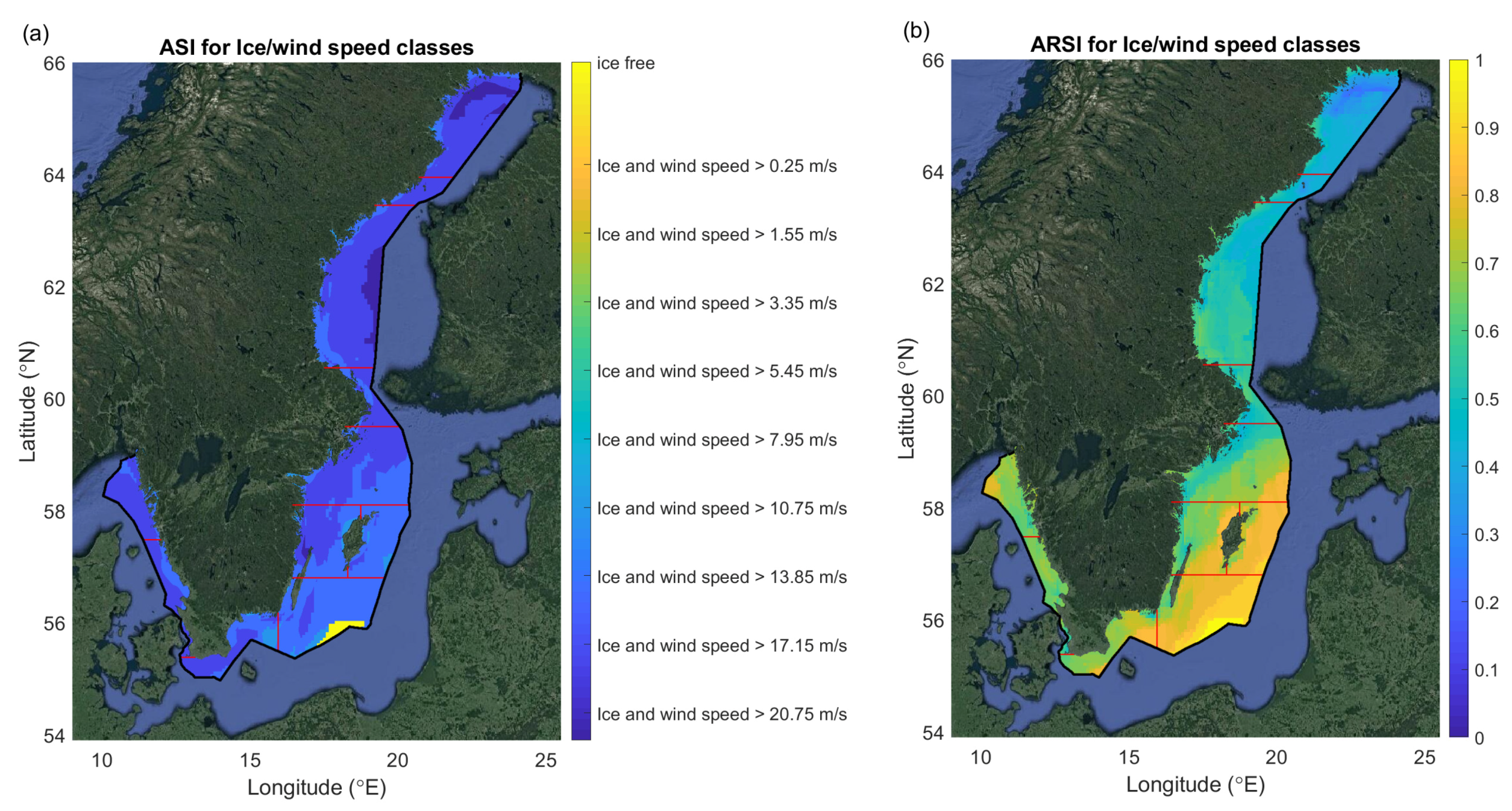
4.1.3. Suitability Index Based on Ice/Wind Speed Classes

The average suitability index for ice/wind speed categories in Figure 8a partly resembles the ASI for ice concentration in Figure 6a in the sense that only a small area in the southeastern SEEZ with yellow color is completely ice-free and hence always assigned a suitability index value of one regardless of the wind speed. Other areas have various shades of blue colors with only a few regions having more greenish color. This is because most areas had at some point in time between 1980 and 2013 wind speeds up to above moderate and fresh breeze conditions during some type of ice condition. The average suitability index would hence for many of the ice/wind speed categories be marked as potentially critical in this type of assessment; however, this type of information did not reflect how often the conditions took place, and a relative scale was also useful to study. The information provided by the ASI was however that wind speeds up to about 8 to 11 m/s were fairly common during ice-condition and that marine infrastructure should be designed to hold for the potential loads these conditions could imply. For the higher ice/wind speed categories corresponding to gale and storm conditions, they were more uncommon and because of this reason also difficult to predict the probability of, but areas of higher occurrence of sea-ice would have a higher risk of obtaining these types of compound events that impose some of the harshest metocean conditions in the Baltic Sea region.

The average relative suitability index in Figure 8b also shows a fairly consistent picture with the assessment of the ice thickness and ice concentration ARSI emphasizing that south of latitude ${60}^{\circ }$ N or ${59}^{\circ }$ N, the best conditions for most ice/wind speed categories are found in a relative sense. This is due to less average ice-time essentially regardless of which category is considered. Some coastal regions will however experience more frequent occurrences and can receive classifications similar to what is typical in Basins 3 and 4.

Correlation analysis was conducted between the individual suitability indexes of different ice/wind speed categories, and for neighboring categories, high correlations were typically obtained, with the light air and light breeze category having the highest 0.99, implying non-sensitivity for results in exact choices between two categories of different, but fairly similar wind speed. The only category for which the individual relative suitability index did not show good correlation with other categories was for the strong gale and ice conditions because these were rare and only occurred over small areas. The correlations ranged between 0.20 for the strong gale category to the light air category up to 0.32 between the fresh and strong gale relative SI. For the relative suitability index of fresh gale and ice, which was also a rare occurrence category, the correlation to the light air results was still 0.61 and to the neighboring moderate gale results as high as 0.81. The results for moderate gale to lower wind speed results gave correlation coefficients between 0.73 and 0.89. This meant that the average relative SI results in Figure 8b could be argued to some extent to represent the overall view of the ice/wind speed aspect of individual suitability indexes, apart from the rare compound events of winds above fresh or strong gale force during ice conditions, which may need further study outside the scope of this investigation.

4.1.4. Suitability Index Based on Significant Wave Height and Wave Power

The average relative suitability index for significant wave height is shown in Figure 9a and for wave power in (b) based on the percentiles shown in Figure 5. The two ARSI were highly correlated and showed in general a very similar picture as shown by the mean wave power statistic for SEEZ and Baltic Sea region in Figure 4 in [6]. This aspect was thoroughly examined and discussed for the SEEZ in terms of the physical dependence of wave power resource on distance from coast, fetch, dominant wave directions, etc., for different basins in [6].

Here, we investigated further how well different percentile results of the distributions could be used to formulate suitability indexes that represented the described overall picture. It may be important to discuss because different wave energy technologies may take advantage of different ranges of the wave heights and power distributions, and hence, we may ask to what extent similarity in relative suitability existed and whether results and conclusions drawn from an average suitability pattern could be representative for individual SI or not. Individual suitability indexes may of course be easier to formulate once specific choices on technology have been made, but for this study of prevailing metocean conditions within the SEEZ, we avoided to as large extent as possible making specific choices about technologies because there exists a wide variety of different types of technologies (e.g., [1,2]) suitable for a wide variety of different marine conditions.

In metocean studies, it is common to study the percentiles of wave height or so-called combined power matrices of wave heights and wave periods. Such data have also been derived for the SEEZ region and have been used in the SWERM project for a more specific study of technical wave energy potential [7]. It should be noted that here, we chose to display the significant wave height results with the notion that it was a positive aspect to have high waves, because we considered that for sites within fairly sheltered seas with 99.9th percentiles typically below 6–7 m, these ranges of wave heights would likely not threaten the survivability of wave energy converters, at least not for some of the technologies mentioned in Section 4.1. Even lower wave heights would, however, as we will later see, affect the number of weather windows and waiting periods for O&M activities, but these aspects will be studied separately in the following sections.

The correlation analysis of all relative suitability indexes for the significant wave height aspect revealed a high degree of similarity for all categories with the lowest linear correlation coefficient being 0.87 between the 25th and 99.9th percentile results. The highest correlation of 0.99 was found between the 90th and 95th percentile essentially indicating the same relative suitability classification for the same areas with regards to the significant wave height aspect. For the wave power investigation, the results were found to be very similar to the lowest correlation of 0.85 also found between the 25th and 99.9th percentile results, indicating a large degree of similarity.

4.2. Operations and Maintenance Conditions within SEEZ

From previous sections, it was clear that ice conditions occurred in especially the northern parts and some coastal regions of the SEEZ, and it became reasonable to consider some ice conditions as potentially critical for O&M activities in addition to if the significant wave heights were high. As discussed in [4,24], different access limits applied for different WECs and marine vessels, and the work in [61] discussed that different types of boat landings or motion-compensating landing systems could be utilized, making limits in the range of 0.5 to 3 m significant wave height relevant to discuss for defining weather windows and waiting periods for wind energy purposes. Less studied is wave energy with regards to these aspects, but the work in [24] used a limit of 2 m significant wave height in a global overview of accessibility around the coasts of the world. Here, we apply several limits ranging between 0.5 and 4 m, but for clarity show results for 1, 2, and 3 m and for simplicity illustrate the differences between if the conditions when the wave model sees ice (>30% concentration) are considered as critical or not for the O&M activity. The access limit of 3 m significant wave height is as previously discussed a fairly high threshold for sea operations for crews and divers, but may in the future not be limiting for ROVs and AUVs. No definition of what ice conditions is surely critical has been established, and further research is needed to determine this, but is considered outside the scope of the present study. The no-ice statistics will hence illustrate a pattern with higher accessibility depending on the ice-free distributions of wave conditions only, and this is useful as it can be combined with other choices of ice aspects and their suitability indexes (see Section 4.4) at a later stage, if found applicable. The ice-included statistic directly illustrated a reduction in weather windows and an increase in waiting periods as expected for some regions and gave a more direct combined view on which basins were affected significantly by ice, and which were not.

Figure 10a shows the average number of 24 h long weather windows per year as a function of the spatial percentile for the SEEZ, indicating how many percentage points of of the region had the presented number of WW. For increasing significant wave heights considered as critical conditions, the number of WWs increased, and the ice conditions of course decreased the number of days. It is worth noting that for both considering ice and no-ice, the number of weather windows when a significant wave height limit of 3 m was considered at least 75% of the SEEZ region would have more than about 330 WWs per year on average. If wave heights less than 3 m were considered critical for the O&M activities, the number of weather windows decreased significantly in most areas, and this indicated that to achieve good accessibility to sites in most places with limited ice, the marine infrastructure should be designed to handle these conditions when possible; otherwise, the risk of long waiting periods for the next WW to occur also increased significantly.

Figure 10b illustrates how long the mean waiting periods became for different access limits chosen on significant wave height and if ice was considered as an inhibiting factor or not. Regardless if ice was considered or not, the mean waiting periods were typically short, about 2.1 days, for at least 75% of the SEEZ if significant wave heights less than 2 m were considered as acceptable weather conditions. A limit of 2 m is also used at the Swedish Meteorological and Hydrological Institute when guiding and providing route planning for naval cargo vessels in the Baltic Sea operationally. Lower waves are typically of little concern to cargo and maintenance vessels, but as discussed, operation safety for crew and divers may be concerned with this limit. Lower wave conditions are more frequent (see Figure 5) and became relevant to consider as potentially critical also for smaller rubber boats and recreational vessels. Warnings for severe and extreme wave conditions in the Baltic Sea from the Finnish Meteorological Institute are also issued together with other meteorological warnings seven times a day, or more often when needed. The thresholds used are 2.5 m, 4 m, and 7 m significant wave height [75], where the 7 m wave height is considered dangerous for all ships and the lowest threshold is important for smaller boats.

When it comes to waiting periods, it does of course not only become relevant to note what the average waiting period is, but also in what a higher percentile (see Figure 10c) corresponding to a type of extreme case scenario may result. If ice was assumed to not be an inhibiting factor for the O&M activities, 75% of the SEEZ region had a 99th percentile waiting period of less than about three days for a significant wave height limit of 3 m, but increased to about 6.4 (24.5) days for a limit of 2 (1) m. If equipment fails and needs to be repaired, these longer waiting periods may cause unnecessary production loss of wave energy converters. Site accessibility may thus be significantly reduced if marine vessels not dimensioned for intermediately high wave conditions are being used. For the scenario with ice as an inhibiting factor, the waiting periods increased; however, 50% of the SEEZ region had less than 10 (6) days as their 99th percentile waiting period at access limits of 2 (3) m, and the results were, as we will later see, latitude dependent.

4.2.1. Weather Windows and Accessibility

For the assessment of weather windows, it could make sense to formulate suitability indexes directly to illustrate if there are any regions with very many 24 h weather windows, which is highly advantageous over areas with less frequent opportunity to site visits and O&M activities. If we chose a threshold of more than 347 weather windows per year on average, this implied that 95% of the time, the site should be accessible. Doing so and taking the average of those SI for the different studied choices (1, 2 and 3 m) resulted in Figure 11a,c for if ice was considered as an inhibiting factor or not, respectively. Some areas around coastlines showed yellow colors, indicating that even when 1 m access limits were considered, the number of weather windows was above 347 days per year. This was an effect of the low wave climate at these sites, but in terms of accessibility, this could be viewed as a positive aspect. Even larger areas shown in green indicated regions in which at least 347 weather windows per year were found on average if marine infrastructure and vessels were used that could handle 2 m significant wave heights. A clear distinction was here recognized between Figure 11a,c with a large reduction in green areas above about latitude ${59}^{\circ }$ N in (a) when ice was considered as an inhibiting factor. For a choice of technology that could utilize conditions with significant wave heights, also up to 3 m further expanded the areas assessed to reach 347 weather windows per year to all the light blue colored areas. This choice almost covered the entire non-coastal SEEZ region when ice was not considered an inhibiting factor (in c). There were only a few dark blue areas left in the southeastern part of the SEEZ in the Baltic proper basin and in the outer edges of the SEEZ region in Basin 11 on the Swedish west coast. Hence, a high accessibility was reached essentially everywhere when ice was not a concern; however, from (a), we note that especially Basins 1 and 2 and the northern part of Basin 3 indicated less accessibility related to the ice-cover. This was also indicated around very near-shore coastal regions on especially the less wind-exposed east coast of Sweden, which was expected and in agreement with the general picture given by the various average relative suitability indexes for ice conditions presented in Section 4.1.

To further differentiate between which areas that were in a relative sense better and worse when it came to the number of weather windows (and thereby accessibility), we formulated relative suitability indexes for all choices of inhibiting limits in terms of significant wave height and if ice was to be considered inhibiting or not. The ARSI with ice as the inhibiting factor and not is shown in Figure 11b,d, respectively.

From Figure 11d, a clear picture emerges with high values of up to one near coasts due to the low wave climate of those sites, but we can also note clearly the difference between the east and west coast due to the higher near-shore wave climate on the west coast of Sweden related to the predominant southwesterly wind directions [6] as a feature of the synoptic weather situation of the Baltic Sea region. Only further offshore in the southeastern part of the SEEZ in Basin 5 and on the west coast region of Basin 11, darkish blue colored areas showed up as a consequence of the higher wave climate with also higher wave power (see Figure 9). Given that this was a relative classification, we should recognize from Figure 11c that high accessibility of more than 95% could in fact likely be reached also for these regions if infrastructure, marine vessels, and operation safety requirements are not limited by wave heights less than 3 m. On a relative scale like this, which is useful to identify sites that are better and worse, we note that high similarity was reached between the individual suitability indexes ranging from 0.93 to 0.97 in the linear correlation coefficient, implying the method to classify sites was not sensitive if only wave height distributions were a concern and not ice conditions.

The results of Figure 11b, when ice was taken into account as an inhibiting factor in addition to the choices of wave height access limits, show a fairly similar pattern as in (d), but with the northern Basins 1 and 2 and part of 3 recognized together with some coastal areas as less suitable in terms of the studied accessibility aspect. With these regions recognized as in a relative sense less good, some of the other areas would switch to higher relative suitability and even become recognized to be in the top 95th percentile in terms of the number of weather windows and hence be assigned yellow color in the figure. There were some larger differences between especially the pattern emerging from the choice of 1 m significant wave height and the other choices, but for the choice of 2 and 3 m, the linear correlation coefficient between their respective suitability indexes was fairly high, 0.82, indicating quite strong similarity in patterns for these wave heights. These conditions may also be reasonable to consider the accessibility when it comes to O&M activities given that many marine vessels can operate in these circumstances and few would be limited by as low wave heights as 1 m.

4.2.2. Waiting Periods

Site accessibility is governed partly by how long of a time marine vessels need to wait for acceptable weather conditions to perform the desired O&M activity. It is hence advantageous to have short waiting periods both in the mean and in extreme cases. If ice was assumed as not inhibiting activities, the significant wave height was mainly governing the assessment of acceptable conditions. In Figure 12a,c, we assigned a value of one if mean waiting periods for the winter season (December to February) were less than three days and else a value of zero for each SI and then averaged across all indexes. We considered the winter period here as it was the season with the longest waiting periods both because of more ice conditions, as well as in some regions a higher probability for higher wave conditions due to increased extra-tropical cyclone activity. Other seasons almost exclusively showed results of very high site accessibility (not shown here) except for some occurrences with stormy weather starting in November followed by either early ice formation or further high wave conditions in the winter season.

From Figure 12c, we note that when ice was not an inhibiting factor, all wave height limitations, even the one corresponding to 1 m, would not make mean waiting periods longer than three days. For the green areas, the mean waiting periods were longer than three days for such a low significant wave height limit of 1 m, but not for the 2 and 3 m results. From Figure 12a, the results changed around some coastlines and in the northern basins as ice was considered as an additional limiting factor. For the dark blue areas, the ice conditions implied longer than a three day mean waiting period even for all wave height limits considered (1, 2, and 3 m), but more importantly, we note that quite large areas of yellow and green colors remained with unchanged results and a high accessibility with mean waiting periods below three days even during the winter.

The average relative SI with regards to mean waiting periods in Figure 12b,d recognized largely the same areas, as better and worse, as the results previously shown for weather windows. Overall, the same areas south of latitude ${59}^{\circ }$ N were assigned the yellow or orange colors corresponding to values close to one, but when ice was a limiting factor, the results in the northern basins that typically had lower wave heights obtained a different pattern, shown in (b).

When it comes to waiting periods in winter-time, not only the mean behavior is of interest to discuss, but also the risk of having longer, but more rare events when ice and wave conditions cause long waiting periods of several weeks. We chose to study this aspect using the 99th percentile waiting period for December to January following Guanche et al. [24] in Figure 13 and repeated the analysis conducted for the mean waiting period.

The average suitability indexes in Figure 13a,c were formulated based on if the 99th percentile waiting period was longer or shorter than three weeks. The yellow colors in (c) hence implied that if ice was not an inhibiting factor, the 99th percentile waiting periods were always less than three weeks even for the case of considering 1 m as the limiting significant wave height. The green areas showed less than three weeks for the 99th percentile waiting period if 2 m significant wave heights were acceptable weather conditions for defining a WW. If ice was a limiting factor, the picture changed quite dramatically north than about latitude ${59}^{\circ }$ N with most places showing a 99th percentile waiting period greater than three weeks for any of our choices of significant wave height limits (1, 2, and 3 m), indicated by the dark blue area. As in previous results, the southern basins were however much less affected, and increases in waiting periods took place mostly around some coastal regions, while many other areas remained with unchanged results and low risk of long waiting periods. The average relative SI based on the 99th percentile waiting periods shown in Figure 13b,d showed similar results as for mean waiting periods (in Figure 12), implying a non-sensitivity to the analysis results and relative assessment of better and worse regions when it came to the aspect of waiting periods. Correlation analysis of the individual relative suitability indexes also showed linear correlation for no ice conditions between 0.88 and 0.96, and for ice as an inhibiting factor, the correlation between the 2 m and 3 m results was also very high between 0.91 and 0.95, indicating that the picture did not differ much in a relative classification of sites dependent on these choices.

4.3. Extreme Value Analysis with a Focus on the SEEZ

Figure 14 reveals that uncertainty existed with regards to 100 year return values for significant wave heights. The methods applied showed some areas with high return values (above 10 m) in both the shorter (16 year) and the longer (44 and 45 year) datasets indicated by red lines (marked A and D). The exact locations that showed return levels above a given threshold differed somewhat both depending on the model setup that generated the different datasets, as well as for some regions, but smaller differences depending on if the POT method or annual maxima method was used (not shown). The high-resolution dataset showed some regions close to the coast with a higher than 10 m return level (marked B, C, and F), which the other coarser resolution datasets did not show. The dataset from Weisse et al. [52] showed some higher wave conditions in the eastern part of the central Baltic Sea (marked E), which the other two datasets did not show. Nevertheless, some areas both on the Swedish west coast in Basin 11 and in the southern part of Basin 8 showed consistently estimated 100 year return levels above 10 m and locally up to 12 m.

These should be considered high values considering the highest observed significant wave height in the Baltic Sea of 8.3 m, and the highest probable may have reached up to 9.5 m during the wind storm Gudrun in 2005 [75,76]. The evaluation of 95th percentile values of significant wave height within or near the SEEZ also revealed a small overestimation in [6], but we are not aware of the evaluation of the dataset from Weisse et al. [52] and Reistad et al. [51] considering extreme values in the Baltic Sea. When the modeled datasets included such high values (of 8 or 9 m) and the datasets were only 16 or even 45 years long, fitting the GEV distribution or GP distribution would, however, result in higher values estimated for a 100 year return level. This is useful information that can be used conservatively in design criteria. In such a context, it is often important to use a higher than observed value conservatively considering that the life-time of offshore structures may often be about 20 to 30 years and measurement records are typically shorter.

The 100 year return level is also sometimes used in the site selection process [67]. Here, we could use a multi-model ensemble to estimate the likely areas to have higher extreme waves and classify these on some relative scale to formulate a suitability index. However, this may become too restrictive in the sense that the areas of highest extreme waves also often coincide with areas of high wave energy potential within the SEEZ [6]. Instead, it is noted that overall, the estimated extreme values for the SEEZ were actually relatively low in comparison to for instance the North Atlantic Ocean [33] or Irish and Scottish coastlines, and given that many wave energy converters are developed to handle those more severe conditions, a 100 year return level of 12 m may be considered not necessarily to impose much of a restriction for many developed technologies. To reach more certain estimates of extreme values within the SEEZ and the Baltic Sea, further work would be needed with high-resolution modeling for very long time periods and potentially using ensembles to better account for uncertainties in models.

Given the differences between model datasets (and smaller differences between methods) to estimate extremes, it may be worth noting that the 8 m return level from any dataset appeared to encapsulate almost all the areas with 10 m estimates that different models showed (except for some small areas often close to the coast). With the lack of additional information and taking a conservative approach, many areas with shown return levels above 8 m may actually be considered to have a risk of significant wave heights also up to 10 m, when taking into account the confidence levels and modeling uncertainties of extreme conditions.

4.4. Correlation and Joint Analysis between Different Aspects

We observed in previous sections that correlation existed between several different aspects, and here, we quantify this using the linear correlation coefficient between the average relative suitability index for different aspects shown in the elements below the diagonal in

Table 1. The correlation (below diagonal) and percentage of nodes within the SEEZ with the average relative suitability index above 0.4 (above diagonal) for both combined aspects given by the first row and first column. The aspects considered are: scaled Relative Classes from Nilsson et al. [6] (RC), wave Power (P), Ice Concentration (IC), Ice Thickness (IT), Ice/Wind Speed (IWS), significant wave height (${\mathit{H}}_{\mathit{s}}$), Weather Windows (WW), weather windows (ignoring ice) (${\mathit{WW}}_{\mathit{ni}}$), mean Waiting Periods (WP), and mean waiting periods (ignoring ice) (${\mathit{WP}}_{\mathit{ni}}$).

	RC	P	IC	IT	IWS	${\mathit{H}}_{\mathit{s}}$	WW	${\mathit{WW}}_{\mathit{ni}}$	WP	${\mathit{WP}}_{\mathit{ni}}$
RC	-	45%	46%	47%	48%	44%	38%	23%	46%	23%
P	0.60	-	67%	70%	75%	77%	62%	53%	69%	53%
IC	0.66	0.75	-	75%	75%	66%	65%	50%	74%	50%
IT	0.69	0.70	0.96	-	82%	70%	72%	56%	77%	57%
IWS	0.65	0.64	0.94	0.91	-	75%	80%	69%	78%	69%
${\mathit{H}}_{\mathit{s}}$	0.58	0.99	0.74	0.69	0.63	-	62%	52%	68%	53%
WW	−0.04	−0.40	0.07	0.22	0.11	−0.42	-	65%	69%	65%
${\mathit{WW}}_{\mathit{ni}}$	−0.59	−0.98	−0.75	−0.70	−0.65	−0.99	0.40	-	53%	74%
WP	0.29	0.55	0.55	0.68	0.51	0.14	0.76	−0.16	-	53%
${\mathit{WP}}_{\mathit{ni}}$	−0.63	−0.81	−0.81	−0.77	−0.71	−0.97	0.32	0.98	−0.24	-

. It is important to note both aspects that were highly correlated (0.99) such as the wave Power (P) and significant wave height ($H_s$) and strongly negatively correlated (−0.98) such as wave power and weather windows for the scenario of ignoring sea-ice ($W{W}_{ni}$), so-called no-ice statistics. This is a consequence of two diametrically opposed aspects as high waves are advantageous because of the increase in wave power this results in, but disadvantageous if this results in a large reduction in the number of weather windows available for O&M activities. For such a case, one possibility is to study the variation in one aspect conditional on the other aspect. This was done in [6] for the aspect of wave power and distance from the coast with the creation of a relative classification based on the amount of annual mean wave power compared to typical at a given distance from coast. We included here in the analysis also this Relative Classification (RC) aspect, but for consistency, we divided the relative classes by a factor five to place it in a range from zero to one. The relative wave power resource classification is also shown in Figure 15, with the colored lines explained later.

Studying the correlation between different aspects, we note that aspects related to different ice properties (concentration, thickness, and ice/wind speed) were all highly correlated (between 0.91 to 0.96), which implied to a large extent that there was not always a large independence between these aspects, and areas could be assessed for relative suitability based on one aspect alone and expect to reach a similar result from the other aspects. This was also reflected in their connection to other aspects, for instance the correlation between ice aspects and relative classes had a reasonably high correlation in the range of 0.65 to 0.69 and a low correlation with the number of weather windows (0.07 to 0.22). There was however a fairly high correlation between the ARSI for ice concentration and wave power of 0.75, which reduced to 0.70 for ice thickness and 0.64 for the ice/wind speed aspect. This may partly be expected because the wave modeling used ice concentration in determining if ice existed or not during its modeling, but not information of ice thickness or high wind speed ice conditions. Hence, it made sense in an overall assessment of metocean conditions to include many aspects when possible as some degree of independence existed.

If no or little independence existed between two aspects, we could simplify and use one aspect when identifying areas that were in a relative sense more suitable for wave energy than others because the same areas would be identified by both suitability indexes. In the above diagonal elements of Table 1, we display the percentage of nodes in the Swedish Exclusive Economic Zone that had ARSI above 0.4 for both the aspect given by the first row and first column. That corresponded roughly to the area that was remaining after ignoring some of the (in relative terms) worst conditions based on two aspects alone and keeping both the better and more typical average conditions. It became evident when studying these percentages that the weather windows and waiting period aspects especially when formulated to ignore the ice conditions would typically reduce the percentages significantly. As an example, combining the Relative Classification (RC) with the weather window no-ice aspect ($W{W}_{ni}$) or similar waiting period aspect ($W{P}_{ni}$) would reduce the number of remaining nodes to 23%. This was a consequence of the previously mentioned opposing effects of high waves being both advantageous and disadvantageous, consistent with the fairly strong negative correlations between these aspects of −0.59 and −0.63, respectively. Some aspects combined in this way however left a high remaining amount of area, which was expected, for instance 82% between ice thickness and ice/wind speed classes, which signified that they were identifying more or less the same areas as having worse and better ice conditions. The 80% remaining nodes between the aspects of weather windows and ice/wind speed conditions may at first be less intuitive, but was a consequence of mainly two things. Firstly, the number of weather windows was significantly reduced by ice, and secondly, the areas that had less WW due to high waves in the offshore open sea conditions usually had higher wind speed as well.

When combining all studied aspects as a preliminary analysis of better and worse overall conditions for wave energy, the requesting ARSI to be above 0.4, and the relative wave power resource from [6] to have Class 3 or higher, we obtained the areas encircled by black lines in Figure 15. These areas were inclusive of almost all the areas encircled by red lines previously discussed in [6] when it came to the Baltic Sea. For the west coast of Sweden in Basin 11, we noticed however that this approach would exclude many areas that were not very close to the coast. This was because the areas with the highest wave conditions would have reduced the relative suitability with respect to WWs and waiting periods. On the west coast of Sweden, there were more fairly high waves closer to the coast, and because of this, the black lines would only encircle a small area. We should remember however that if safety requirements were met and naval vessels and marine infrastructure were designed to deal with conditions of significant wave height of 3 m, the waiting periods were typically short, and the number of weather windows was in fact quite appealing everywhere for the sheltered seas of Sweden. It may therefore make more sense to remove the limitations imposed by the $W{P}_{ni}$ and $W{W}_{ni}$ aspects. The areas identified after doing this remained with an unchanged inner border close to coasts (as the black line) because of multiple drawbacks of increased ice conditions and reduced wave power. However, the identified area extended outward to the blue line because only areas with even higher waves than this would have a similar level of reduction in weather windows and an increase in mean waiting periods, as was caused by sea-ice in the northern basins and along some coastal regions.

We note that with this choice based on an ARSI of above 0.4 for all aspects (that took ice into account), also the previously discussed smaller areas encircled by red lines from [6] were included on the west coast of Sweden, as well as fully included in the Baltic Sea basins. This illustrated the interesting point that when looking at aspects in a relative sense, certain basins may appear less or more suitable depending on the presence of how conditions were in another basin. It therefore became important to note that if the areas outside of the blue lines were deemed to have reasonably good accessibility, not too large transmission losses [7], and acceptable extreme wave conditions that could be handled by the specific technology and infrastructure planned for in a wave energy project, then also these regions could be further considered because they had some of the highest wave energy potential within the SEEZ [6,7].

The areas encircled by the red lines should hence be seen as mainly illustrating a case of near-shore suitable areas that was based on the previous experience from pilot sites being located closer than 20 km from the coast. In the sheltered conditions of the Baltic Sea region, also less restrictive choices may potentially prove useful, but also environmental factors, sea-floor conditions, and several technical aspects are further studied within the SWERM project. A final weighting of different aspects as in for instance [67] will also be applied at a later stage within the SWERM project, possibly ranking sites for their overall average suitability as wave energy sites.

5. Summary and Conclusions

The metocean conditions for the Swedish Exclusive Economic Zone were investigated with regards to multiple aspects relevant for establishment of wave energy.

• Both a high-resolution one-kilometer wave hindcast dataset and two lower resolution datasets of 5.5 km and about 10–11 km were used to study extreme wave conditions within the SEEZ. The relatively high 100 year return level values for significant wave height of above 10 m predicted for some areas by all datasets could be used as a conservative estimate of the design criteria of WECs and other marine infrastructure.
• Except for these extreme wave conditions, the investigation of the 99.9th percentiles of significant wave height showed that most sites would very rarely reach threshold limits corresponding to the survival modes of WECs of about 6 m or higher in the sheltered seas of the SEEZ.
• A strong similarity in the relative suitability was found with regards to ice concentration occurrence within the SEEZ, as well as a high correlation between different ice aspects (concentration, thickness, and ice/wind speed classes). This signified some insensitivity about the final results on the thresholds used in the investigation.
• Thin ice of less than about 15 cm thickness is fairly frequently encountered over wide-spread areas of the SEEZ, and it is advisable that marine infrastructure and vessels be adapted to handle these situations even if intended to operate only in the southern basins of the Baltic Sea.
• Wind speeds up to about 8 to 11 m/s during ice conditions are fairly common in the Baltic Sea region, which could be expected as winter months typically have higher wind speeds prevailing due to the extra-tropical cyclone activity on the middle-latitudes. Higher wind speed categories corresponding to gale and storm strengths are uncommon in combination with sea-ice; however, the probability of such compound events is difficult to assess, and further study is needed as these conditions impose some of the harshest metocean conditions of the Baltic Sea.
• Excellent accessibility with many weather windows and short waiting periods could be achieved at most sites for the study area if marine infrastructure were designed for access limits for significant wave heights up to 3 m and safety requirements for operations at sea could be met at those wave heights.
• A joint analysis of average relative suitability indexes for multiple aspects illustrated a methodology that could be used in the site selection process, but only preliminary results were shown here, as additional aspects are being studied within the national Swedish Wave Energy Resource Mapping (SWERM) project. These will also include technical wave energy aspects, environmental factors, and geotechnical assessment of sea-floor conditions, among other things. The methods, results, and the large number of geo-spatial data fields generated and presented here could be used to answer questions about the prevailing metocean conditions of the SEEZ and are useful information for planning of energy projects both as pilot sites or on a larger commercial-scale, as well as useful for planning of other marine activities.

References

1. Drew, B.; Plummer, A.R.; Sahinkaya, M.N. A review of wave energy converter technology. Proc. Inst. Mech. Eng. Part A J. Power Energy 2009, 223, 887–902. [Google Scholar] [CrossRef] [Green Version]
2. Rusu, E.; Onea, F. A review of the technologies for wave energy extraction. Clean Energy 2018, 2, 10–19. [Google Scholar] [CrossRef] [Green Version]
3. Magagna, D.; Uihlein, A. Ocean energy development in Europe: Current status and future perspectives. Int. J. Mar. Energy 2015, 11, 84–104. [Google Scholar] [CrossRef]
4. Walker, R.T.; van Nieuwkoop-McCall, J.; Johanning, L.; Parkinson, R.J. Calculating weather windows: Application to transit, installation and the implications on deployment success. Ocean Eng. 2013, 68, 88–101. [Google Scholar] [CrossRef]
5. Strömstedt, E.; Haikonen, K.; Engström, J.; Götman, M.; Sundberg, J.; Nyberg, J.; Zillén-Snowball, L.; Nilsson, E.; Dingwell, A.; Rutgersson, A. On defining wave energy pilot sites in Swedish Seawaters. In Proceedings of the 12th European Wave and Tidal Energy Conference (EWTEC), Cork, Ireland, 27 August–1 September 2017. [Google Scholar]
6. Nilsson, E.; Rutgersson, A.; Dingwell, A.; Björkqvist, J.V.; Pettersson, H.; Axell, L.; Nyberg, J.; Strömstedt, E. Characterization of Wave Energy Potential for the Baltic Sea with Focus on the Swedish Exclusive Economic Zone. Energies 2019, 12, 793. [Google Scholar] [CrossRef] [Green Version]
7. Engström, J.; Göteman, M.; Eriksson, M.; Bergkvist, M.; Nilsson, E.; Rutgersson, A.; Strömstedt, E. Energy absorption from parks of point-absorbing wave energy converters in the Swedish exclusive economic zone. Energy Sci. Eng. 2020, 8, 38–49. [Google Scholar] [CrossRef]
8. Castellucci, V.; Strömstedt, E. Sea level variability in the Swedish Exclusive Economic Zone and adjacent seawaters: Influence on a point absorbing wave energy converter. Ocean Sci. 2019, 15, 1517–1529. [Google Scholar] [CrossRef] [Green Version]
9. Morim, J.; Cartwright, N.; Etemad-Shahidi, A.; Strauss, D.; Hemer, M. Wave energy resource assessment along the Southeast coast of Australia on the basis of a 31-year hindcast. Appl. Energy 2016, 184, 276–297. [Google Scholar] [CrossRef]
10. Bernardino, M.; Rusu, L.; Soares, C.G. Evaluation of the wave energy resources in the Cape Verde Islands. Renew. Energy 2017, 101, 316–326. [Google Scholar] [CrossRef]
11. Akpınar, A.; Bingölbali, B.; Vledder, G.P.V. Long-term analysis of wave power potential in the Black Sea, based on 31-year SWAN simulations. Ocean Eng. 2017, 130, 482–497. [Google Scholar] [CrossRef]
12. Kovaleva, O.; Eelsalu, M.; Soomere, T. Hot-spots of large wave energy resources in relatively sheltered sections of the Baltic Sea coast. Renew. Sustain. Energy Rev. 2017, 74, 424–437. [Google Scholar] [CrossRef]
13. Farhadzadeh, A.; Hashemi, M.R.; Neill, S. Characterizing the Great Lakes hydrokinetic renewable energy resource: Lake Erie wave, surge and seiche characteristics. Energy 2017, 128, 661–675. [Google Scholar] [CrossRef] [Green Version]
14. Chen, X.; Wang, K.; Zhang, Z.; Zeng, Y.; Zhang, Y.; O’Driscoll, K. An assessment of wind and wave climate as potential sources of renewable energy in the nearshore Shenzhen coastal zone of the South China Sea. Energy 2017, 134, 789–801. [Google Scholar] [CrossRef] [Green Version]
15. Kasiulis, E.; Kofoed, J.P.; Povilaitis, A.; Radzevičius, A. Spatial Distribution of the Baltic Sea Near-Shore Wave Power Potential along the Coast of Klaipėda, Lithuania. Energies 2017, 10, 2170. [Google Scholar] [CrossRef] [Green Version]
16. Liberti, L.; Carillo, A.; Sannino, G. Wave energy resource assessment in the Mediterranean, the Italian perspective. Renew. Energy 2013, 50, 938–949. [Google Scholar] [CrossRef]
17. Langodan, S.; Viswanadhapalli, Y.; Dasari, H.P.; Knio, O.; Hoteit, I. A high-resolution assessment of wind and wave energy potentials in the Red Sea. Appl. Energy 2016, 181, 244–255. [Google Scholar] [CrossRef]
18. Besio, G.; Mentaschi, L.; Mazzino, A. Wave energy resource assessment in the Mediterranean Sea on the basis of a 35-year hindcast. Energy 2016, 94, 50–63. [Google Scholar] [CrossRef]
19. Aboobacker, V.; Shanas, P.; Alsaafani, M.; Albarakati, A.M. Wave energy resource assessment for Red Sea. Renew. Energy 2017, 114, 46–58. [Google Scholar] [CrossRef]
20. Amirinia, G.; Kamranzad, B.; Mafi, S. Wind and wave energy potential in southern Caspian Sea using uncertainty analysis. Energy 2017, 120, 332–345. [Google Scholar] [CrossRef]
21. Kamranzad, B. Persian Gulf zone classification based on the wind and wave climate variability. Ocean Eng. 2018, 169, 604–635. [Google Scholar] [CrossRef]
22. Bozzi, S.; Besio, G.; Passoni, G. Wave power technologies for the Mediterranean offshore: Scaling and performance analysis. Coast. Eng. 2018, 136, 130–146. [Google Scholar] [CrossRef]
23. Yang, S.; Fan, L.; Duan, S.; Zheng, C.; Li, X.; Li, H.; Xu, J. Long-term assessment of wave energy in the China Sea using 30-year hindcast data. Energy Explor. Exploit. 2020, 38, 37–56. [Google Scholar] [CrossRef] [Green Version]
24. Guanche, R.; de Andrés, A.; Losada, I.; Vidal, C. A global analysis of the operation and maintenance role on the placing of wave energy farms. Energy Convers. Manag. 2015, 106, 440–456. [Google Scholar] [CrossRef]
25. Gray, A.; Dickens, B.; Bruce, T.; Ashton, I.; Johanning, L. Reliability and O&M sensitivity analysis as a consequence of site specific characteristics for wave energy converters. Ocean Eng. 2017, 141, 493–511. [Google Scholar] [CrossRef]
26. Kahma, K.; Pettersson, H.; Tuomi, L. Scatter diagram wave statistics from the northern Baltic Sea. MERI Rep. Ser. Finn. Inst. Mar. Res. 2003, 49, 15–32. [Google Scholar]
27. Pettersson, H.; Jönsson, A. Wave Climate in the Northern Baltic Sea in 2004; Technical Report, HELCOM Indicator Fact Sheets; Institute of Marine Research: Helsinki, Finland, 2005; Available online: https://helcom.fi/media/documents/Wave-climate-in-the-northern-Baltic-Sea-in-2004.pdf (accessed on 24 February 2020).
28. Broman, B.; Hammarklint, T.; Kalev, R.; Soomere, T.; Valdmann, A. Trends and extremes of wave fields in the north-eastern part of the Baltic Proper. Oceanologia 2006, 48, 165–184. [Google Scholar]
29. Jönsson, A.; Broman, B.; Rahm, L. Variations in the Baltic Sea wave fields. Ocean Eng. 2003, 30, 107–126. [Google Scholar] [CrossRef]
30. Räämet, A.; Soomere, T. The wave climate and its seasonal variability in the northeastern Baltic Sea. Est. J. Earth Sci. 2010, 59, 100–113. [Google Scholar] [CrossRef]
31. Björkqvist, J.V.; Lukas, I.; Alari, V.; van Vledder, G.P.; Hulst, S.; Pettersson, H.; Behrens, A.; Männik, A. Comparing a 41-year model hindcast with decades of wave measurements from the Baltic Sea. Ocean Eng. 2018, 152, 57–71. [Google Scholar] [CrossRef] [Green Version]
32. Soomere, T. Extremes and Decadal Variations of the Northern Baltic Sea Wave Conditions. In Extreme Ocean Waves; Pelinovsky, E., Kharif, C., Eds.; Springer: Dordrecht, The Netherlands, 2008; pp. 139–157. [Google Scholar]
33. Aarnes, O.J.; Breivik, Ø.; Reistad, M. Wave Extremes in the Northeast Atlantic. J. Clim. 2012, 25, 1529–1543. [Google Scholar] [CrossRef] [Green Version]
34. Report: Towards a Baltic Offshore Grid: Connecting Electricity Market through Offshore Wind Farms. 2018. Available online: www.baltic-integrid.eu (accessed on 24 January 2020).
35. Soomere, T.; Eelsalu, M. On the wave energy potential along the eastern Baltic Sea coast. Renew. Energy 2014, 71, 221–233. [Google Scholar] [CrossRef]
36. Bernhoff, H.; Sjöstedt, E.; Leijon, M. Wave energy resources in sheltered sea areas: A case study of the Baltic Sea. Renew. Energy 2006, 31, 2164–2170. [Google Scholar] [CrossRef]
37. Henfridsson, U.; Neimane, V.; Strand, K.; Kapper, R.; Bernhoff, H.; Danielsson, O.; Leijon, M.; Sundberg, J.; Thorburn, K.; Ericsson, E.; et al. Wave energy potential in the Baltic Sea and the Danish part of the North Sea, with reflections on the Skagerrak. Renew. Energy 2007, 32, 2069–2084. [Google Scholar] [CrossRef]
38. Kasiulis, E.; Punys, P.; Kofoed, J.P. Assessment of theoretical near-shore wave power potential along the Lithuanian coast of the Baltic Sea. Renew. Sustain. Energy Rev. 2015, 41, 134–142. [Google Scholar] [CrossRef]
39. Löptien, U.; Dietze, H. Sea ice in the Baltic Sea - revisiting BASIS ice, a historical dataset covering the period 1960/1961–1978/1979. Earth Syst. Sci. Data 2014, 6, 367–374. [Google Scholar] [CrossRef] [Green Version]
40. Tuomi, L.; Kanarik, H.; Björkqvist, J.V.; Marjamaa, R.; Vainio, J.; Hordoir, R.; Höglund, A.; Kahma, K.K. Impact of Ice Data Quality and Treatment on Wave Hindcast Statistics in Seasonally Ice-Covered Seas. Front. Earth Sci. 2019, 7, 166. [Google Scholar] [CrossRef] [Green Version]
41. Tuomi, L.; Kahma, K.; Pettersson, H. Wave hindcast statistics in the seasonally ice-covered Baltic Sea. Boreal Environ. Res. 2011, 16, 451–472. [Google Scholar]
42. Strömstedt, E.; Savin, A.; Heino, H.; Antbrams, K.; Haikonen, K.; Götschel, T. Project WESA (Wave Energy for a Sustainable Archipelago)—A Single Heaving Buoy Wave Energy Converter Operating and Surviving Ice Interaction in the Baltic Sea. In Proceedings of the 10th European Wave and Tidal Energy Conference (EWTEC 2013), Aalborg, Denmark, 2–5 September 2013. [Google Scholar]
43. Savin, A.; Temiz, I.; Strömstedt, E.; Leijon, M. Statistical analysis of power output from a single heaving buoy WEC for different sea states. Mar. Syst. Ocean Technol. 2018, 13, 103–110. [Google Scholar] [CrossRef] [Green Version]
44. Savin, A.; Strömstedt, E.; Leijon, M. Full-Scale Measurement of Reaction Force Caused by Level Ice Interaction on a Buoy Connected to a Wave Energy Converter. J. Cold Reg. Eng. 2019, 33, 04019001. [Google Scholar] [CrossRef]
45. Remouit, F.; Chatzigiannakou, M.; Bender, A.; Temiz, I.; Sundberg, J.; Engström, J. Deployment and Maintenance of Wave Energy Converters at the Lysekil Research Site: A Comparative Study on the Use of Divers and Remotely-Operated Vehicles. J. Mar. Sci. Eng. 2018, 6, 39. [Google Scholar] [CrossRef] [Green Version]
46. Chatzigiannakou, M.A.; Ulvgård, L.; Temiz, I.; Leijon, M. Offshore deployments of wave energy converters by Uppsala University, Sweden. Mar. Syst. Ocean Technol. 2019. [Google Scholar] [CrossRef] [Green Version]
47. The Wamdi Group. The WAM Model-A Third Generation Ocean Wave Prediction Model. J. Phys. Oceanogr. 1988, 18, 1775–1810. [Google Scholar] [CrossRef] [Green Version]
48. Komen, G.J.; Cavaleri, L.; Donelan, M.; Hasselmann, K.; Hasselmann, S.; Janssen, P.A.E.M. Dynamics and Modelling of Ocean Waves; Cambridge University Press: Cambridge, UK, 1994. [Google Scholar] [CrossRef]
49. Guenther, H.; Hasselmann, S.; Janssen, P. The WAM Model Cycle 4; Technical Report; Deutsches KlimaRechenZentrum: Hamburg, Germany, 1992. [Google Scholar]
50. Iuppa, C.; Cavallaro, L.; Vicinanza, D.; Foti, E. Investigation of suitable sites for wave energy converters around Sicily (Italy). Ocean Sci. 2015, 11, 543–557. [Google Scholar] [CrossRef] [Green Version]
51. Reistad, M.; Breivik, Ø.; Haakenstad, H.; Aarnes, O.; Furevik, B. A High-Resolution Hindcast of Wind and Waves for the North Sea, the Norwegian Sea and the Barents Sea; Technical Report, Norwegian Meteorological Institute Research Report No. 2009/14; Meteorologisk Institutt: Oslo, Norway, 2009. [Google Scholar]
52. Weisse, R.; von Storch, H.; Callies, U.; Chrastansky, A.; Feser, F.; Grabemann, I.; Günther, H.; Pluess, A.; Stoye, T.; Tellkamp, J.; et al. Regional Meteorological-Marine Reanalyses and Climate Change Projections. Bull. Am. Meteorol. Soc. 2009, 90, 849–860. [Google Scholar] [CrossRef] [Green Version]
53. Weisse, R.; Gaslikova, L.; Geyer, B.; Groll, N.; Meyer, E. coastDat—Model Data for Science and Industry. Die Küste 2014, 81, 5–18. [Google Scholar]
54. Różyński, G. Long-term evolution of Baltic Sea wave climate near a coastal segment in Poland; its drivers and impacts. Ocean Eng. 2010, 37, 186–199. [Google Scholar] [CrossRef]
55. Bömer, J.; Brodersen, N.; Hunke, D.; Schüler, V.; Günther, H.; Weisse, R.; Fischer, J.; Schäffer, M.; Gaßner, H. Ocean Energy in Germany. Executive Summary. 2010. Available online: https://www.coastdat.de/imperia/md/content/coastdat/ecofys_2010_ocean_energy_in_germany.pdf (accessed on 24 February 2020).
56. Uiboupin, R.; Axell, L.; Raudsepp, U.; Sipelgas, L. Comparison of operational ice charts with satellite based ice concentration products in the Baltic Sea. In Proceedings of the 2010 IEEE/OES Baltic International Symposium (BALTIC), Riga, Latvia, 25–27 August 2010; pp. 1–8. [Google Scholar] [CrossRef]
57. Barua, D.K. Beaufort Wind Scale. In Encyclopedia of Coastal Science; Springer: Dordrecht, The Netherlands, 2005; p. 186. [Google Scholar] [CrossRef]
58. Undén, P.; Rontu, L.; Järvinen, H.; Lynch, P.; Calvo, J.; Cats, G.; Cuaxart, J.; Eerola, K.; Fortelius, C.; Garcia-Moya, J.; et al. HIRLAM-5 Scientific Documentation; Technical Report, HIRLAM-5 Project, S-601767; SMHI: Norrköping, Sweden, 2002. [Google Scholar]
59. Dahlgren, P.; Kållberg, P.; Landelius, T.; Undén, P. EURO4M Project Report, D 2.9 Comparison of the Regional Reanalyses Products with Newly Developed and Existing State-of-the Art Systems; Technical Report; SMHI: Norrköping, Sweden, 2014. [Google Scholar]
60. O’Connor, M.; Lewis, T.; Dalton, G. Weather Window Analysis of Irish and Portuguese Wave Data with Relevance to Operations and Maintenance of Marine Renewables. In Proceedings of the ASME 2013 32nd International Conference on Ocean, Offshore and Arctic Engineering, Nantes, France, 9–14 June 2013. [Google Scholar]
61. Tveiten, C.K.; Albrechtsen, E.; Heggset, J.; Hofmann, M.; Jersin, E.; Leira, B.; Norddal, P.K. Hse Challenges Related to Offshore Renewable Energy; Report, A18107; SINTEF Technology and Society: Trondheim, Norway, 2011. [Google Scholar]
62. O’Connor, M.; Lewis, T.; Dalton, G. Weather window analysis of Irish west coast wave data with relevance to operations & maintenance of marine renewables. Renew. Energy 2013, 52, 57–66. [Google Scholar] [CrossRef]
63. Antonelli, G.; Fossen, T.I.; Yoerger, D.R. Underwater Robotics. In Springer Handbook of Robotics; Springer: Berlin/Heidelberg, Germany, 2008; pp. 987–1008. [Google Scholar] [CrossRef]
64. Sivčev, S.; Coleman, J.; Omerdić, E.; Dooly, G.; Toal, D. Underwater manipulators: A review. Ocean Eng. 2018, 163, 431–450. [Google Scholar] [CrossRef]
65. Coles, S. An Introduction to Statistical Modeling of Extreme Values; Springer Series in Statistics; Springer: London, UK, 2001. [Google Scholar] [CrossRef]
66. Gutjahr, O.; Heinemann, G. A model-based comparison of extreme winds in the Arctic and around Greenland. Int. J. Climatol. 2018, 38, 5272–5292. [Google Scholar] [CrossRef] [Green Version]
67. Flocard, F.; Ierodiaconou, D.; Coghlan, I.R. Multi-criteria evaluation of wave energy projects on the south-east Australian coast. Renew. Energy 2016, 99, 80–94. [Google Scholar] [CrossRef]
68. Weber, J.E. Steady Wind- and Wave-Induced Currents in the Open Ocean. J. Phys. Oceanogr. 1983, 13, 524–530. [Google Scholar] [CrossRef] [Green Version]
69. Chang, Y.C.; Chen, G.Y.; Tseng, R.S.; Centurioni, L.R.; Chu, P.C. Observed near-surface currents under high wind speeds. J. Geophys. Res. Ocean. 2012, 117. [Google Scholar] [CrossRef]
70. Park, H.S.; Stewart, A.L. An analytical model for wind-driven Arctic summer sea ice drift. Cryosphere 2016, 10, 227–244. [Google Scholar] [CrossRef] [Green Version]
71. World Meteorological Organization. WMO Sea-Ice Nomenclature, Terminology, Codes and Illustrated Glossary; Technical Report, (WMO/OMM/BMO 259, TP 145); World Meteorological Organization: Geneva, Switzerland, 1970. [Google Scholar]
72. Rashid, A.; Hasanzadeh, S. Status and potentials of offshore wave energy resources in Chahbahar area (NW Omman Sea). Renew. Sustain. Energy Rev. 2011, 15, 4876–4883. [Google Scholar] [CrossRef]
73. Wavestar. 2015. Available online: http://wavestarenergy.com/ (accessed on 28 April 2015).
74. Saulnier, J. Deliverable 6: Annual Variability of Wave Energy; Technical Report, Marie Curie Actions, MRTN-CT-2004-50166; Instituto Nacional de Engenharia, Tecnologia e Inovação, I.P: Lisboa, Portugal, 2007. [Google Scholar]
75. Björkqvist, J.V.; Tuomi, L.; Tollman, N.; Kangas, A.; Pettersson, H.; Marjamaa, R.; Jokinen, H.; Fortelius, C. Brief communication: Characteristic properties of extreme wave events observed in the northern Baltic Proper, Baltic Sea. Nat. Hazards Earth Syst. Sci. 2017, 17, 1653–1658. [Google Scholar] [CrossRef] [Green Version]
76. Soomere, T.; Behrens, A.; Tuomi, L.; Nielsen, J.W. Wave conditions in the Baltic Proper and in the Gulf of Finland during windstorm Gudrun. Nat. Hazards Earth Syst. Sci. 2008, 8, 37–46. [Google Scholar] [CrossRef]
Figure 1. Subdivision of the Swedish Exclusive Economic Zone (SEEZ) into 11 smaller basins indicated by the number and different colors following [6].
Atmosphere 11 00229 g001
Figure 2. Sketch of the methodology going from geo-spatial data to classifications based on either yes/no (potentially critical/non-critical) conditions or on a relative scale based on the frequency of occurrence or intensity of the aspect considered. For the relative scale, a value of one can be assigned to all areas for which a non-occurrence of the aspect considered has taken place, to result in an Suitability Index (SI) ranging between zero and one, or six classes can be presented based on percentile limits. Averaging across suitability indexes corresponding to many different choices to formulate an average SI is advantageous as a first assessment of metocean conditions for a region, before specific choices about technology and marine infrastructure to be used in a project have been made. All individual SI results for different choices will however also be saved for a full description of metocean conditions, which may be needed at a project level.
Atmosphere 11 00229 g002
Figure 3. Percent of SEEZ that had presence of different types of ice conditions. Three aspects (ice thickness, ice concentration, and wind speed classes during ice) are represented with three different x-axes in blue, red, and black, respectively.
Atmosphere 11 00229 g003
Figure 4. Percentile values for the average number of days per year with regards to selected ice thickness classes (in (a)), ice concentration (conc.) classes (in (b)), and wind speed classes during ice conditions (in (c)). The wind speed classes were created based on an adapted Beaufort scale [57], and ice concentration classes were based on the WMO sea-ice classes [71], while ice thickness categories were created for every 5 cm; however, only selected lines corresponding to the lowest and thickest considered ice classes are shown here to increase the clarity of the figure.
Atmosphere 11 00229 g004
Figure 5. Percentile values for ice-free significant wave height (in (a)) and wave power P (in (b)) are shown against the spatial percentile for the SEEZ indicating how many percentage points of the region have the presented significant wave height or wave power conditions.
Atmosphere 11 00229 g005
Figure 6. The Average Suitability Index (ASI) for Ice Concentration (IC) based on considering any presence of ice classes (in (a)) represents the presence of their maximum ice concentration category over 34 years. The percentile limits of Figure 4b are used to formulate the Average Relative Suitability Index (ARSI) in (b), which takes into account the amount of time of various ice concentration categories. A value of one indicates ice-free or non-critical ice concentration conditions for all categories considered, and low values imply the presence of potentially critical ice concentration conditions for many of the categories (or thresholds) considered. Sub-basin borders following Figure 1 are marked with red lines.
Atmosphere 11 00229 g006
Figure 7. The Average Suitability Index (ASI) for Ice Thickness (IT) based on considering any presence of ice thickness categories (in (a)) represents the presence of their maximum ice thickness category over 34 years. The percentile limits are used to formulate the Average Relative Suitability Index (ARSI) in (b), which takes into account the amount of time of various ice thickness categories. A value of one indicates ice-free or non-critical ice thickness conditions for all categories considered, and low values imply the presence of potentially critical ice thickness conditions for many of the categories considered. Sub-basin borders following Figure 1 are marked with red lines.
Atmosphere 11 00229 g007
Figure 8. The ASI for the ice/wind speed aspect based on considering any presence of ice and wind speed categories (in (a)) and considering the percentile limits (in Figure 4c) to formulate the ARSI in (b). A value of one indicates ice-free or non-critical wind speed during ice conditions for all categories considered, and low values imply the presence of potentially critical wind speed during ice conditions for many of the categories considered. Sub-basin borders following Figure 1 are marked with red lines.
Atmosphere 11 00229 g008
Figure 9. The ARSI for ice-free significant wave height (in (a)) and for ice-free wave power resource (in (b)) formulated based on the percentile limits in Figure 5. A value of one indicates that the area has been classified to have the 5% highest waves and wave power in all categories considered, and low values indicate the areas that have the lowest wave heights and wave power values for many of the categories considered. Sub-basin borders following Figure 1 are marked with red lines.
Atmosphere 11 00229 g009
Figure 10. The number of 24 h weather windows (in (a)), length of mean waiting periods (in (b)), and 99th percentile waiting periods (in (c)) shown as a function of the spatial percentile for the SEEZ, indicating how many percentage points of the region that have the considered number of weather windows and length of waiting periods. Different significant wave height limits are used together with assumptions that ice conditions are considered as inhibiting (blue lines) or not (black lines) for the assessment of weather windows.
Atmosphere 11 00229 g010
Figure 11. The ASI for weather windows based on considering if the number of weather windows was above or below 347 per year for each of the categories (in (a,c)) and considering the percentile limits to formulate the ARSI in (b,d). The sub-plots (a,b) refer to considering the ice seen by the wave model as inhibiting for defining weather windows, and (c,d) are the corresponding figures assuming ice is not inhibiting O&M activities. A value of one indicates the best weather window conditions for all categories considered, and low values imply the presence of a reduced number of weather windows (WW) for many of the categories considered.
Atmosphere 11 00229 g011
Figure 12. The ASI for mean Waiting Periods (WP) based on considering if the length of mean waiting periods was above or below three days for each of the categories (in (a,c)) and considering the percentile limits to formulate the ARSI in (b,d). The sub-plots (a,b) refer to considering the ice seen by the wave model as inhibiting when defining waiting periods, and (c,d) are the corresponding figures assuming ice is not inhibiting O&M activities. A value of one indicates the best mean waiting period conditions for all categories considered, and low values imply the presence of longer waiting period for many of the categories considered.
Atmosphere 11 00229 g012
Figure 13. The ASI for 99th percentile waiting periods based on considering if the length of the waiting periods was above or below three weeks for each of the categories (in (a,c)) and considering the percentile limits to formulate the ARSI in (b,d). The sub-plots (a,b) refer to considering the ice seen by the wave model as inhibiting when defining waiting periods, and (c,d) are the corresponding figures assuming ice is not inhibiting O&M activities. A value of one indicates the best regions with regards to the 99th percentile waiting periods for all categories considered, and low values imply the presence of longer waiting period for many of the categories considered.
Atmosphere 11 00229 g013
Figure 14. The 100 year return value for the significant wave height from a Peaks-Over-Threshold (POT) method is shown for the SEEZ region with red iso-lines marking values above 10 m and black above 8 m. The background colored field and dashed lines show the results from the high-resolution dataset from [6]. The red and black full lines show the results from a 45 year dataset from [52] and dotted lines from a 44 year dataset from [51]. Some places are marked with symbols A-F for further discussion in the main text.
Atmosphere 11 00229 g014
Figure 15. Relative classification of the wave power resource [6] in five categories comparing the power at sites relative to typical annual mean values for its given distance from the coast. Red lines correspond to the identified areas based on the criteria used in [6]; black lines encircle larger identified areas when including the choices for average relative suitability index for weather windows and waiting periods ignoring ice. This area extends further offshore to the blue line if those choices are excluded from the analysis. See Section 4.4 for further discussion.
Atmosphere 11 00229 g015