Article

Radar-Based Precipitation Climatology in Germany—Developments, Uncertainties and Potentials

1
Institute of Physical Geography and Landscape Ecology, Leibniz Universität Hannover, Schneiderberg 50, 30167 Hannover, Germany
2
Institute of Bio- and Geosciences IBG-3, Forschungszentrum Jülich GmbH, 52425 Jülich, Germany
3
Leibniz Centre for Agricultural Landscape Research ZALF, Eberswalder Straße 84, 15374 Müncheberg, Germany
*
Author to whom correspondence should be addressed.
Atmosphere 2020, 11(2), 217; https://doi.org/10.3390/atmos11020217
Submission received: 30 January 2020 / Revised: 11 February 2020 / Accepted: 19 February 2020 / Published: 21 February 2020
(This article belongs to the Special Issue Radar Hydrology and QPE Uncertainties)

Abstract

:
Precipitation is a crucial driver for many environmental processes and weather radars are capable of providing precipitation information with high spatial and temporal resolution. However, radar-based quantitative precipitation estimates (QPE) are also subject to various potential uncertainties. This study explored the development, uncertainties and potentials of the hourly operational German radar-based and gauge-adjusted QPE called RADOLAN and its reanalyzed radar climatology dataset named RADKLIM in comparison to ground-truth rain gauge data. The precipitation datasets were statistically analyzed across various time scales ranging from annual and seasonal aggregations to hourly rainfall intensities in regard to their capability to map long-term precipitation distribution, to detect low intensity rainfall and to capture heavy rainfall. Moreover, the impacts of season, orography and distance from the radar on long-term precipitation sums were examined in order to evaluate dataset performance and to describe inherent biases. Results revealed that both radar products tend to underestimate total precipitation sums and particularly high intensity rainfall. However, our analyses also showed significant improvements throughout the RADOLAN time series as well as major advances through the climatologic reanalysis regarding the correction of typical radar artefacts, orographic and winter precipitation as well as range-dependent attenuation.

1. Introduction

Precipitation is one of the main drivers of hydrologic and energy cycles and induces a variety of environmental processes such as runoff, erosion or floods and has been acknowledged as an Essential Climate Variable. Due to the high spatiotemporal variability of precipitation, a spatially distributed quantitative estimation of rainfall rates is a challenging task. Thus, the “unbiased estimation of high temporal resolution precipitation amount, especially over the oceans, and over areas of complex orography” [1] has been identified as an outstanding scientific and technological challenge.
Direct rainfall measurements with rain gauges on the ground can only provide local point scale information. As rain gauges are scarce in many regions, this approach is not sufficient to capture spatial rainfall distribution, especially for smaller-scale convective storm events [2,3,4]. In the last decades, ground-based weather radar and space-borne satellite observations have emerged as alternative measurement techniques capable of producing temporally and spatially highly resolved gridded precipitation estimates. Despite their undisputed potential to satisfy the increasing demand of research and planning institutions, insurance companies, policy and operational communities for reliable, highly resolved precipitation data, these data also cause new uncertainties [5]. Both remote sensing-based products are estimates derived from indirect measurements, which are subject to various potential sampling errors causing systematic bias and random errors [6]. Consequently, there are numerous studies that have evaluated radar [7,8,9,10,11,12,13] and satellite [14] products against rain gauges, conducted comparisons between radar and satellite products [15,16,17,18] or between all three methods [19,20].
An excellent overview of radar basics and the main sources of uncertainty is given in [21], whereas [22] provides an overview of the basics and uncertainties of satellite observations. However, up to now, satellite-based quantitative precipitation estimates (QPE) have been less suitable for climatological analyses due to their comparably low spatial and/or temporal resolution [23].
The uncertainties in QPE derived from C-Band radars in the midlatitudes include various different effects, many of them causing an underestimation of rainfall depth. The attenuation of the radar beam by heavy precipitation or a wet radome can lead to a decrease in reflectivity with increasing distance from the radar. The conversion from the measured reflectivity to precipitation depths is hampered by the vertical variability of the drop size distribution and the non-uniform vertical profile of reflectivity. Moreover, the radar beam can be (partially) blocked by obstacles such as buildings or mountains, which cause linear artifacts of regions with underestimated rainfall, the so-called negative spokes. In areas with a diverse and in some regions, complex terrain such as Germany and especially during the winter season, precipitation quantification is a challenge due to differing hydrometeor types, bright-band effects and overshooting. The higher proportion of snow and ice particles at higher altitudes and during wintertime can cause bright-band effects at the melting layer and lead to strong reflectivity signals, whereas the signal above the bright-band may decrease significantly. Moreover, especially rainfall of stratiform and orographic character can be underestimated due to overshooting, which is a source of uncertainty in mountainous areas and at long ranges from the radar caused by the increasing height of observation due to the beam elevation angle and the Earth’s curvature [9,24].
Besides the main sources of uncertainty and various potentials of radar data for hydrological applications, Berne and Krajewski [21] also stated in 2013 that radar data are not used as extensively in the field of hydrology as one would expect. This also holds true for the operational radar-based and gauge-adjusted German QPEs, which have been operationally derived and continuously further developed by the German Weather Service (Deutscher Wetterdienst, DWD) since June 2006 within the RADOLAN (“Radar Online Adjustment”) programme [25]. Despite the fact that these temporally (up to 5 min) and spatially (1 km2) highly resolved data have been available for fourteen years now, RADOLAN is still sparsely used in scientific studies. Studies using RADOLAN comprise the analysis of extreme flash floods and heavy rainfalls [26,27], forecasting of water levels and floods [12,28], the intercomparison to satellite-based QPEs [16,18] and the estimation of rainfall erosivity [29,30]. However, an increased use of RADOLAN data could be observed as most of these studies have been published within the last four years. This tendency might go along with an improvement of data quality since the correction and adjustment algorithms used for RADOLAN have been continuously further developed. In 2018, the radar-based QPE time series was extended back to the year 2001 and reanalyzed using consistent processing techniques and several new correction algorithms. The resulting dataset called RADKLIM (“Radar Climatology”) should open up new climatological application fields for radar composite data such as statistical heavy rainfall analyses, erosion modelling and the use of aggregated precipitation sums for precipitation statistics or as model inputs. Up to now, this dataset has primarily been used by the DWD itself for studies on heavy rainfall frequency and extent [31,32], but also for rainfall erosivity analyses [33,34].
However, to the best of the authors’ knowledge, no nationwide evaluation of the RADOLAN and RADKLIM composites and their inherent error structure has been published yet. This study provides a nationwide comparative evaluation of the recently published RADKLIM dataset in comparison to RADOLAN and rain gauge data. The aim was not to provide a quantitative error matrix, which would require much more independent reference data. Instead, we wanted to map out the differences, developments, advantages and shortcomings of the compared datasets and gain a better understanding of the systematic and random error structure of the RADKLIM and RADOLAN radar composite datasets.
The goal of this study was to support a user’s decision on which of the datasets is best suited depending on the individual study area, time period and intended application and to raise awareness of the potential bias that varies in space and time. Special attention was paid to developments in the RADOLAN processing routines and their impact on data quality as well as to the impacts of the additional correction algorithms applied to derive the RADKLIM dataset.
Resulting from the issues outlined above, the following research questions were addressed and discussed in this study:
  • Which developments in the German radar-based QPE derivation procedure have taken place since the launch of the RADOLAN programme in 2006 and how did they affect data quality?
  • How did the additional climatological correction algorithms used for RADKLIM affect the data quality compared to RADOLAN and the gauge dataset?
  • Which challenges, advantages and limitations do users need to take into account when using RADKLIM and RADOLAN in comparison to gauge data?

2. Materials and Methods
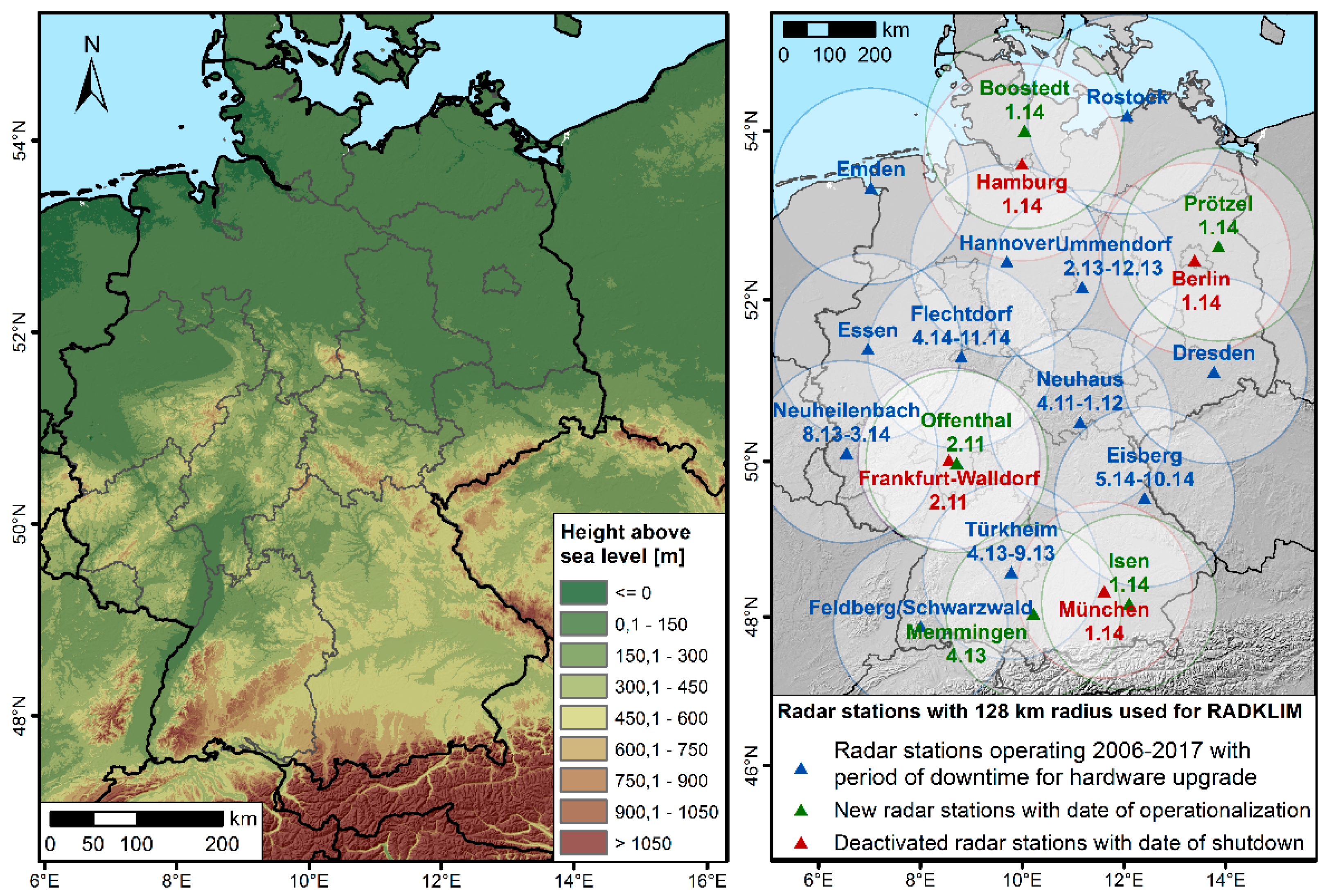
2.1. Study Area

The investigated area for this study comprises the state territory of Germany (see Figure 1), which covers about 357,021 km2 extending from 47° N to 55° N and from 5° E to 16° E. Consequently, the country is located in the humid midlatitudes in a transition zone between a maritime climate in the western part and a humid continental climate in the east. Atmospheric circulation and, thus, the distribution of precipitation is influenced by humid westerly winds, which decrease towards the eastern part of Germany. Additionally, the distribution of precipitation amounts is characterized by the diverse topography of the study area with the summits and foothills of the Alps in the south, a variety of low mountain ranges in the central part and lowlands in the north.

2.2. Data Basis

2.2.1. RADOLAN

The German Weather Service (DWD) operates a network of currently 17 ground-based C-Band radar stations. The reflectivity data obtained by this network have been processed to QPEs on a nationwide 900 km × 900 km grid in 1 km2 resolution within the operational RADOLAN (“Radar Online Adjustment) programme since June 2006.
Data processing and correction algorithms include:
  • The elimination of clutter pixels;
  • Orographic shading correction;
  • Smoothing with gradient filters;
  • A transformation of the reflectivity Z to rain rates R using a custom refined Z-R-relation;
  • Merging the local radar station data to a national gridded composite;
  • The adjustment of the radar-based rain rates to ground-truth automated rain gauge measurements using a weighted average of adjustment differences and factors [25].
The final RADOLAN product RW has an hourly resolution and is freely available at the Open Data DWD server [35] with the most recent interval being provided within 30 min after the end of the measurement interval. The composite with the highest temporal resolution (5 min) is the RY product, which is neither adjusted to gauges nor freely available online.
However, the RADOLAN routine as well as the radar network have been continuously developed, which causes significant changes in the data quality throughout the time series. The first major change in the processing routine took place in December 2007. It comprised the inclusion of foreign gauges and German gauges located close to the border beyond any radar radius as well as a gauge-based interpolation of gaps in the RW product. Two other important changes were the increase of the radar radius from 128 km to 150 km in March 2010 [36,37] and the use of RY data for the derivation of the RW product since May 2010, which introduced additional quality checks for clutter removal and replaced the “push”-method for composite creation by the more mitigating “pull”-method [38,39]. When converting the local radar data in polar projection to a Cartesian composite grid, the size of the polar grid cells becomes larger at longer ranges from the radar. Consequently, close to the radar, several polar cells are located in one Cartesian cell, whereas, at long ranges from the radar, several Cartesian cells may be located within one polar cell. Moreover, in areas with overlapping polar grids, one value has to be selected for the Cartesian grid cell. The “push”-method uses a search radius of one cell in each direction to fill gaps and selects the maximum value of all available values. As a consequence, high values may be spread to all adjacent cells and a characteristic cross-shaped artefact is visible on the composite. The “pull”-method does not apply a search radius and directly selects the value of the closest polar cell. In case of overlaps, the maximum value is selected [40]. In August 2016, a further software update introduced additional clutter corrections, a filter that prevents biased rain gauge values from being used for adjustment, a reduction of edges and inconsistencies at radar borders and additional rain gauges in the Czech Republic for adjustment [41]. Finally, the use of new polarimetric radar data as an input for all composite products since October 2017 constituted the latest major change in the RADOLAN routine [42].

2.2.2. RADKLIM

In 2018, the DWD published a reanalyzed version of their radar reflectivity data archive dating back to the year 2001 using consistent processing techniques and more rain gauges for adjustment [43]. Additionally, new climatological algorithms for the detection and correction of radar-specific artefacts such as clutter and spokes as well as for the correction of signal reduction with distance and height have been developed and applied. In this context, the radius of local radar data used for the composite has been reduced to 128 km. Moreover, the first major change in the RADOLAN routine has been partly revoked for RADKLIM, so that gaps in the radar data are not filled with interpolated gauge data anymore. Instead, gaps are contained in the dataset as no data values. In contrast to the RADOLAN RY product in 5-min resolution, the RADKLIM counterpart called YW [44] has been quasi-adjusted based on the RW product to improve its precipitation quantification. Moreover, the height of the composite has been extended by 200 rows, 100 each in the north and south, and the grid has been shifted eastwards by 80 km in order to cover the entire country and to provide some additional buffer to each side [45].
Table 1 provides an overview of the four final RADOLAN and RADKLIM composite products. Due to the unavailability of the RADOLAN RY product, this study only evaluated the hourly RW products.

2.2.3. Rain Gauge Data

Rain gauge data in 1-min resolution were used as ground-truth precipitation data for validation. These data are freely available in the DWD Open Data Portal [46]. For more details on these data, the processing and the applied quality checks, please refer to [47].

2.3. Methodology

2.3.1. Data Preparation

For the analysis of all precipitation datasets, a processing framework consisting of ArcGIS and Python developed by Kreklow [48] using the radproc version 0.1.4 [49] was used. Moreover, parts of the analyses of this study were based on a rainfall data intercomparison geodataset of RADKLIM, RADOLAN and rain gauge data [50], which provided data pairs of each station and radar pixel for a wide range of precipitation statistics and additional parameters relevant for data quality evaluation.

2.3.2. Dataset Completeness and Outliers

The completeness of the dataset and the occurrence of outliers are two major properties determining the reliability and usability of a dataset as well as the additional effort necessary for raw data processing and data preparation. Both may cause strongly biased precipitation statistics.
In order to assess dataset completeness, the NoData counts, that is, the number of hourly intervals with NoData values, for all 997 gauge-radar data pairs were statistically analyzed.
The occurrence of outliers and their effect on annual precipitation sums were also evaluated based on the intercomparison dataset. Following the definition by Tukey [51], Kreklow et al. [47] defined outliers as annual precipitation sums lying outside 1.5× Interquartile Range (IQR) and calculated cleaned mean annual precipitation (MAP) sums without these outliers. In order to assess the effect of this cleaning process as well as the spatial and temporal distribution of outliers in the datasets, we calculated the differences between cleaned MAP and original MAP.

2.3.3. Precipitation Statistics and Interrelations to Potential Error Sources

Many typical weaknesses of radar measurements such as clutter, spokes and underestimations with increasing distance from the radar and increasing altitude only become apparent through the aggregation of longer time periods. Moreover, the reliable mapping of precipitation amounts is a key requirement for a dataset that is to be used for climatological applications. We put particular emphasis on investigating the seasonal differences between the datasets in order to evaluate the improvements of RADKLIM in quantifying precipitation in winter, when there is a higher prevalence of snowfall.
Thus, precipitation sums and means for varying periods including years, hydrologic half-years, months and days were calculated for each dataset in order to map typical spatial distributions and assess temporal variability. For direct quantitative comparisons, the ratios between RADKLIM and RADOLAN as well as between RADKLIM and gauge data were calculated. All comparative analyses were conducted either for RADKLIM–gauge data pairs (n = 997) or for RADKLIM–RADOLAN pixel pairs (n = 392,529).
In order to assess the level of consistency between the datasets as well as the impacts of altitude and distance from the radar on the QPEs, linear regression models were fitted to the data pairs using the ordinary least squares method and the Pearson correlation coefficient r was calculated for the respective data pairs with the following formula:
r = i = 1 n ( X i X ¯ ) ( Y i Y ¯ ) i = 1 n ( X i X ¯ ) 2   i = 1 n ( Y i Y ¯ ) 2
where X and Y are the respective observed precipitation sums, Y ¯ and X ¯ are the mean precipitation sums, n is the total number of data pairs and i denotes the i th data pair. For the correlation analyses between precipitation sums and altitude or distance from radar, the former is the dependent variable Y and the latter is the independent variable X .
The coefficient of determination r2 was used to evaluate the model fit since it is a measure for the proportion of the variance in the data that can be explained by the model.
r 2 = Model   Sum   of   Squares Total   Sum   of   Squares = i = 1 n ( Y ^ i Y ¯ ) 2 i = 1 n ( Y i Y ¯ ) 2
where Y ^ i is the modeled or predicted value associated to Y i .
For perfect linearity between the datasets, both parameters equal the value 1, whereas values close to 0 indicate a very weak correlation or none at all.
Furthermore, the Root Mean Squared Error (RMSE) was calculated to represent the average magnitude of the error, whereby higher weight is given to larger errors, that is, deviations between the datasets.
RMSE = 1 n i = 1 n ( X i Y i ) 2

2.3.4. Rainfall Detection and Intensity

In addition to the long-term precipitation statistics, the capability to detect rainfall as well as to capture different rainfall intensities up to heavy rainfall was investigated on a daily and hourly time scale for the different precipitation datasets.
On a daily scale, the precipitation detection rate of each precipitation dataset was inferred by counting the days with precipitation sums greater than 1 mm and by calculating the mean precipitation amounts of these rainy days. As an indicator for the capability of a dataset to detect heavy rainfall occurrence, the number of days with precipitation amounts greater than 20 mm and their mean precipitation sums were calculated.
Moreover, the distribution of hourly rainfall intensities was analyzed for RADKLIM and the gauge dataset in order to assess their capability to detect rainfall and to capture rainfall of high intensity. First, the gauge data were resampled from minute to hourly resolutions. Second, all hourly intervals of the resampled gauge dataset and the RADKLIM RW product were classified according to their rainfall intensity and the frequency per class was counted. Finally, the absolute and relative differences of the class frequencies between both datasets were calculated.

3. Results

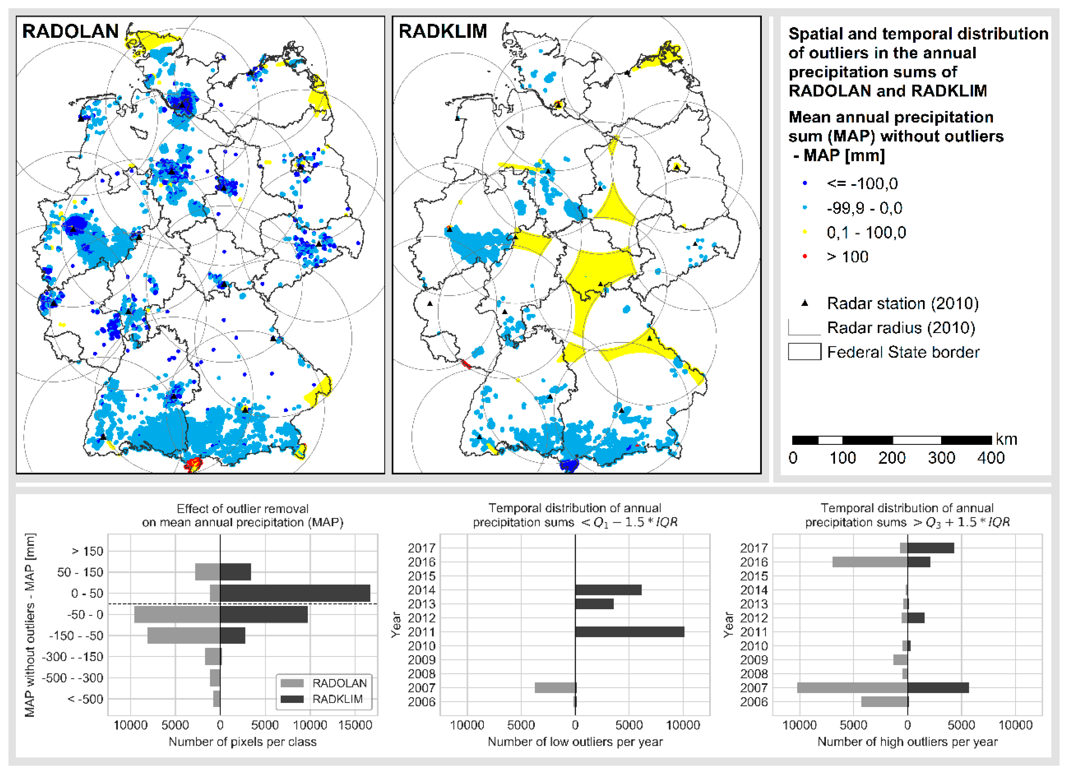
3.1. Spatiotemporal Distribution and Impacts of Outliers and Missing Data

The distribution of outliers varies considerably in space and time as well as between the two datasets. The original RADOLAN data suffer from many high outliers actually causing a positive bias in the mean annual precipitation sum (MAP, see Figure 2). Outliers are particularly frequent at close range around the radars, but also tend to occur in mountainous areas. Visual inspection of the spatial distributions of outliers and wind energy plants revealed that many of the outliers are related to the presence of wind energy plants at the respective pixel if the latter is located at close range to the radar or at mountain ranges. There, the radar beam has a relatively low height above ground and the wind turbine rotors can disturb the radar signal by causing constant noise. These effects could be reduced significantly in RADKLIM.
Figure 2 also shows large areas of low outliers in RADKLIM, which are clearly delineated by radar borders. The occurrence of these data gaps is limited to the years 2011, 2013 and 2014, which correspond to the periods during which some of the radars were replaced by Dual-Pol radars (see Figure 1). These gaps do not occur in RADOLAN since the 150 km radar radia overlap in these areas and there were no temporary backup radars installed while upgrading the operational radars. However, since the radius was reduced to 128 km and the gaps were not filled with interpolated data in RADKLIM, these gaps occur as NoData periods in the RADKLIM dataset. Further reasons for missing data in both radar datasets include radar downtimes due to hardware maintenance work, which is usually conducted during the night in periods without rainfall, as well as several azimuth angles, that may not be scanned by any radar due to radiation protection regulations.
In RADOLAN, low outliers are limited to areas close to the national border that are not covered by any radar. Like the majority of high outliers, they only occur in the years 2006 and 2007, which shows the improvement achieved by the use of additional gauges and the filling of gaps with data interpolated from gauge measurements since December 2007. However, a large portion of the high outliers in RADOLAN and all high outliers in RADKLIM in the very wet year of 2007 can be attributed to a series of heavy rainfall events in central and northern Germany (Figure 2: Light blue dots in RADKLIM map in range of the radars Essen and Hannover) in August and September 2007 [52]. A further decrease of high outliers in RADOLAN could be achieved in 2010 since additional quality checks for clutter removal were introduced and high reflectivity values are no longer spread to the adjacent pixels by the “push”-method when merging and converting local radar data to the gridded Cartesian composite.
The strikingly high number of high outliers in 2016 in both radar datasets, however, was not caused by any changes in the radar data processing but actually by a year of extraordinarily large differences in precipitation distribution. While the overall annual precipitation amount over Germany only reached 93% of the long-term average, Southern Germany suffered from a series of extreme rainfall events in May and June, which caused several flash floods and also casualties. Consequently, most of the light blue pixels in Figure 2 located in the two southernmost Federal States Bavaria (Southeast) and Baden-Württemberg (Southwest) can be associated to these events in 2016, which significantly raised the annual precipitation amount [53].
Similarly, most of the high outliers in RADKLIM in 2017, which are primarily located in Southern Bavaria were caused by a series of heavy rain and snowfall events throughout the entire year and not by radar errors [53]. However, despite the indisputable impact of the heavy rainfalls in Bavaria in the years 2016 and 2017, the increase of values flagged as outliers in this mountainous area in the RADKLIM dataset (especially compared to RADOLAN in 2017) may also be attributed to a better quantification of precipitation in higher altitudes of the Alps, which was additionally improved by a better coverage through the new radar that was established in Memmingen in 2013.

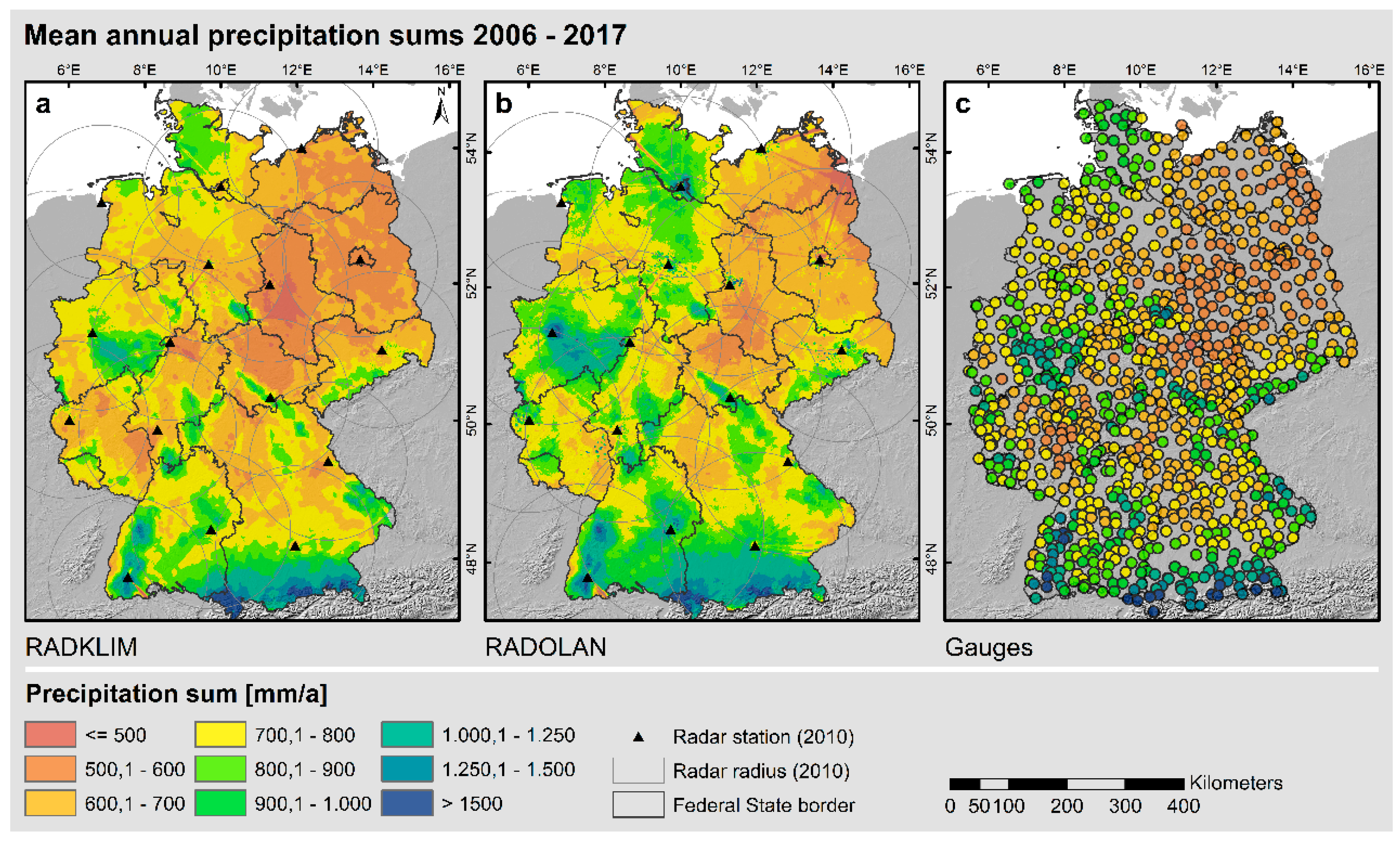
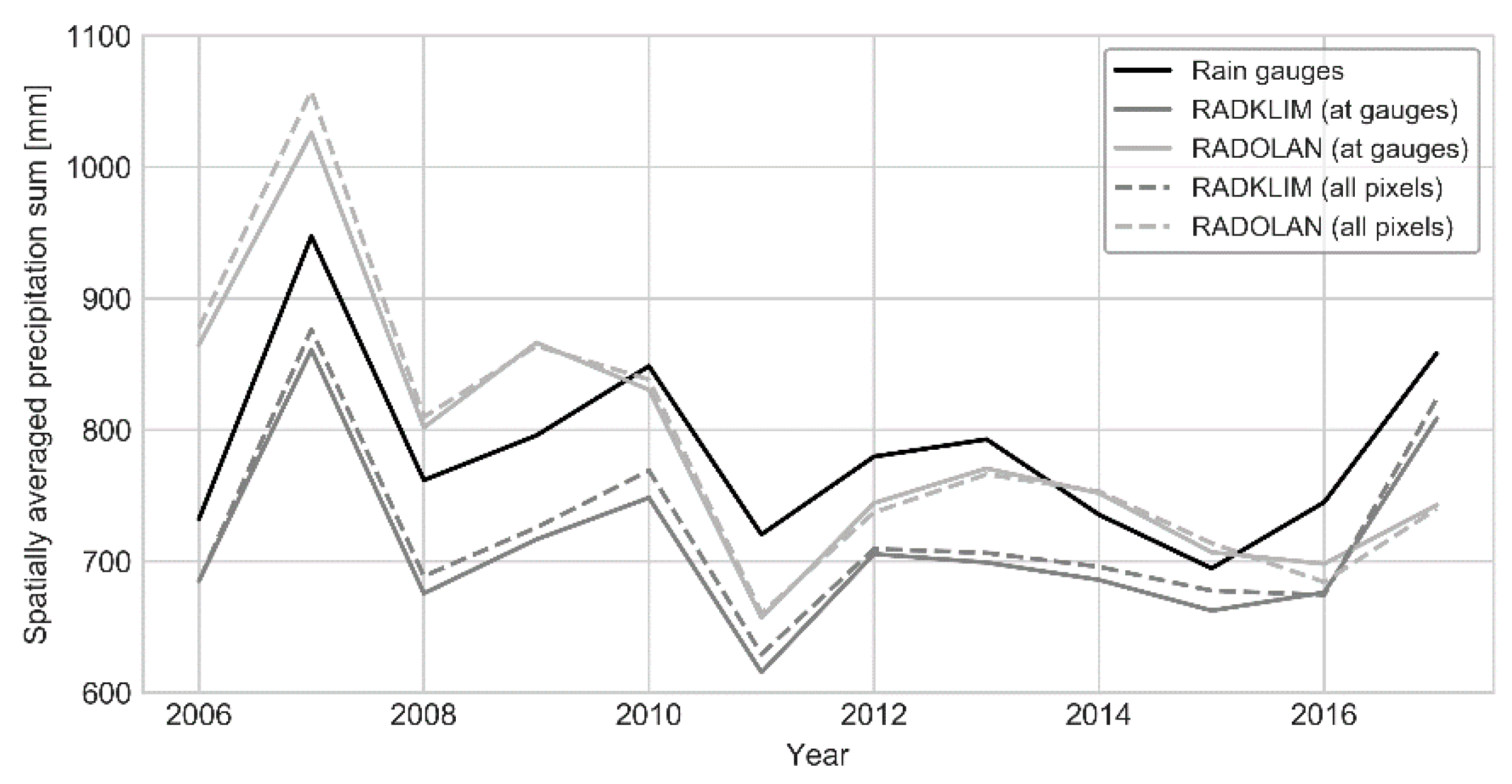
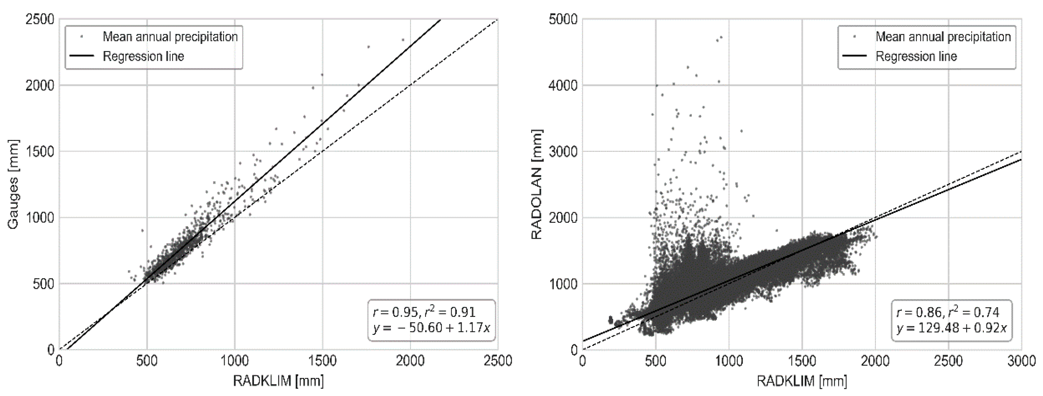
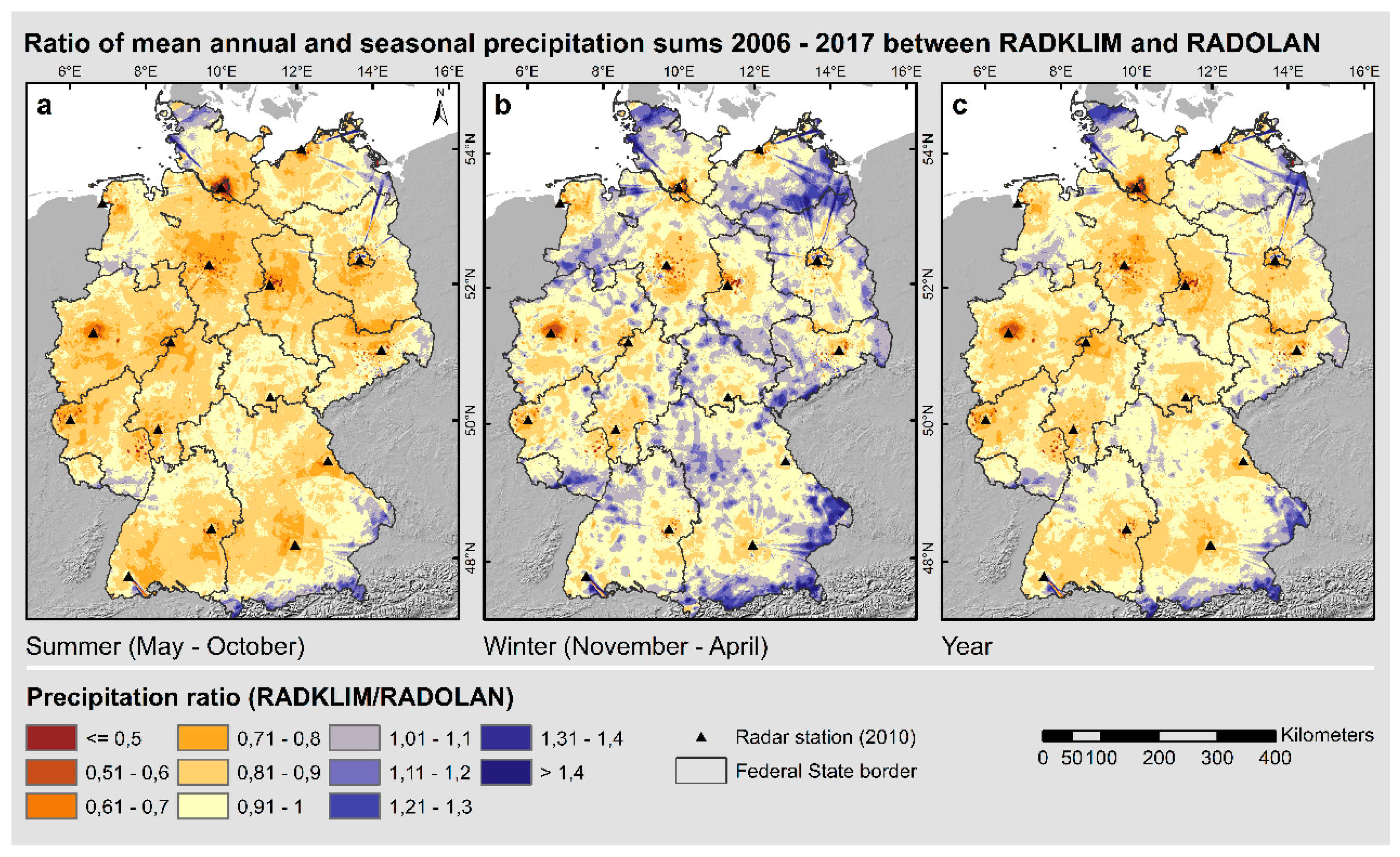
3.2. Annual and Seasonal Precipitation Sums

The overall spatial distribution of the MAP of all three precipitation datasets show similar patterns with mountainous areas being clearly visible and also the transition from a maritime climate in the northwest to a more continental climate with lower precipitation amounts towards the south and east of Germany is well mapped (see Figure 3). However, the actual precipitation amounts differ considerably between the datasets. Taking the gauge MAP of 784.6 mm as a ground-truth, RADKLIM on average underestimates the MAP by 7.9%, whereas RADOLAN overestimates it by 0.9%. The very close match for RADOLAN, however, results from averaging values, which vary heavily in space and time. The temporal development (see Figure 4) shows a significant decrease of precipitation amounts between 2006 and 2011 for RADOLAN, which was caused by the changes in the processing routine discussed above. However, the errors and clutter in the first years of the time series caused such an extreme bias that the maximum MAP in RADOLAN still amounts to 7533 mm and many pixels with very high MAP are located at close range from the radars. These biased MAP values, which could be completely removed in RADKLIM, are also clearly visible in Figure 5.
RADKLIM, on the contrary, shows a much lower MAP, especially in lowland areas in the east and south of Germany. The data gaps identified in the previous section are also clearly visible and explain the very low minimum MAP of 180.9 mm. Moreover, many of the high clutter values around the radars visible in RADOLAN, which are particularly pronounced around the radars in Hannover, Dresden and Frankfurt, were corrected and show below-average values in RADKLIM. In return, many of the spokes, which are clearly visible in RADOLAN, could be successfully corrected in RADKLIM. As a consequence, the overall RADKLIM image shows significantly fewer radar artefacts than RADOLAN. The effects of both corrections (clutter pixels and spokes) became particularly evident by calculating the ratio between RADKLIM and RADOLAN MAP (see Figure 6). The ratio also revealed that almost nationwide the mean summer precipitation sum in RADKLIM is lower than in RADOLAN with the largest differences in close proximity to the radars. During the winter half-year, though, there is a much more differentiated distribution of the ratio. At greater distances from the radars, the ratio becomes positive, so the RADKLIM winter precipitation sums are higher than in RADOLAN. This effect is particularly pronounced in mountainous areas far from the radars. This indicates that the underestimation of precipitation due to attenuation and the lower reflectivity of snowflakes, which are common problems of radar measurements, could be reduced significantly in RADKLIM. Both effects are investigated in more detail in the following section.

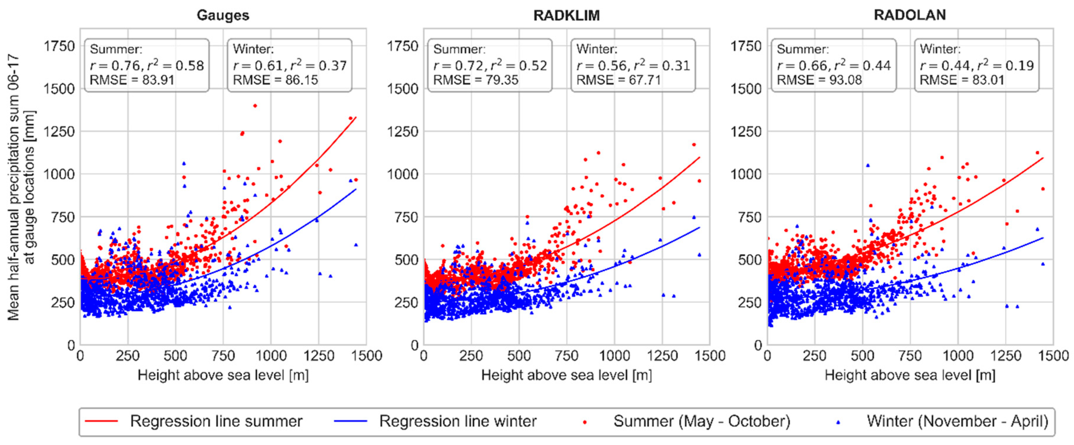
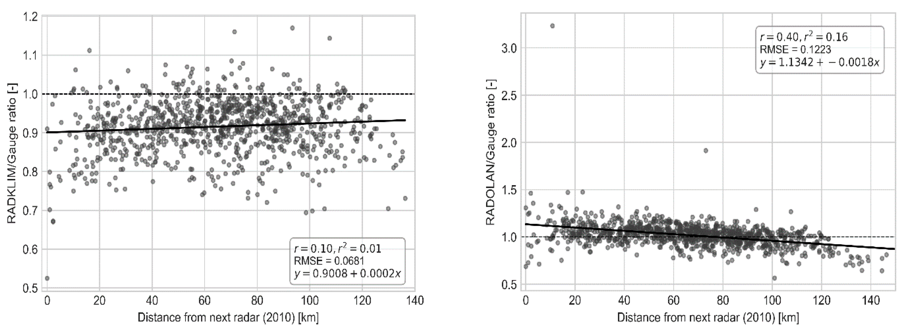
3.3. Impacts of Elevation and Distance from Next Radar

For all three datasets, a quadratic linear regression was best suited to describe the relation between heights above sea level and seasonal precipitation sums (see Figure 7). The better fit of the quadratic model is due to the extraordinarily high elevation of the Alps compared to the rest of Germany, which has a significant positive impact on the precipitation sums. All datasets show higher precipitation sums and correlation coefficients for the summer half-year than for the winter half-year. RADKLIM and the gauge data actually show similar correlation coefficients with a slightly better fit for the gauges and also the RMSEs are almost similar for the summer precipitation sum. For winter, however, the RADKLIM regression line has a more moderate slope and a much lower RMSE indicating less variability in the RADKLIM data. Especially at lower elevations up to about 550 m, the winter precipitation sums of the gauge data tend to be higher than the RADKLIM sums. Both regression lines are less steep for RADKLIM, which indicates that the increase of precipitation amounts with increasing altitude is slightly underestimated in RADKLIM. Furthermore, the higher spread between the summer and winter regression lines shows that this effect is somewhat stronger in winter than in summer. However, these effects are not very pronounced and the overall distributions of gauges and RADKLIM show very similar patterns and both map the increase of precipitation with increasing elevation. The results for RADOLAN, however, show a much poorer performance and coincide with the observations shown in Figure 6. There is a much stronger underestimation of winter precipitation at higher altitudes with a very weak coefficient of determination r2 = 0.19. In summer, the overall relation between precipitation and altitude is comparable to RADKLIM, but less reliable for the individual pixel as the high RMSE indicates.
The impact of the distance from the radar was assessed using the MAP ratios between the radar products and the gauges since these are independent from the actual precipitation amounts. The regression analysis (see Figure 8) showed a significant difference between RADKLIM and RADOLAN in terms of attenuation correction. The RADOLAN/gauge ratio decreases considerably with increasing distance from the next radar. The turning point from a predominantly positive to a predominantly negative ratio is located at an approximately 70 km distance from the radar. Besides some extreme outliers close to the radars, an additional drop of the ratio beyond about 120 km distance from the radar became apparent. In order to assess the impact of the larger radius used for RADOLAN, we removed all 19 value pairs beyond a 128 km distance from the radar and recalculated the regression (not shown). The slope of the recalculated regression line (y = 1.1214 − 0.000015x) differed only slightly from the original regression using the entire value range. The coefficient of determination decreased to r2 = 0.11 and the turning point from predominantly positive to predominantly negative values shifted to an about 80 km distance from the radar. Thus, the larger radius for RADOLAN does have a slight impact on the decrease of radar rainfall at far ranges from the radar, but this decrease is governed by a systematic bias in the RADOLAN data. In contrast to this, with a coefficient of determination of r2 = 0.01, the RADKLIM/gauge ratio shows no correlation at all to the distance from the radar. Instead, independently from the distance to the radar, the ratio averages almost constantly at about 0.91. Consequently, the additional attenuation correction algorithms developed for the radar climatology in conjunction with the decrease of the radar radius to 128 km led to a significant improvement in data quality.

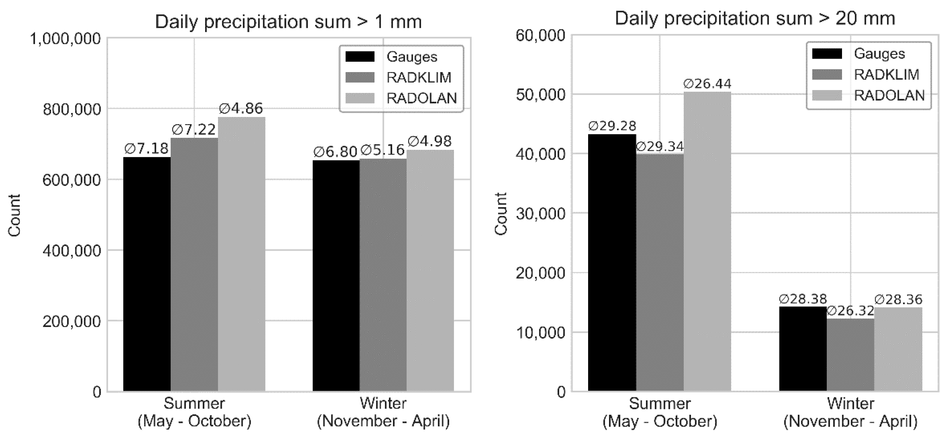
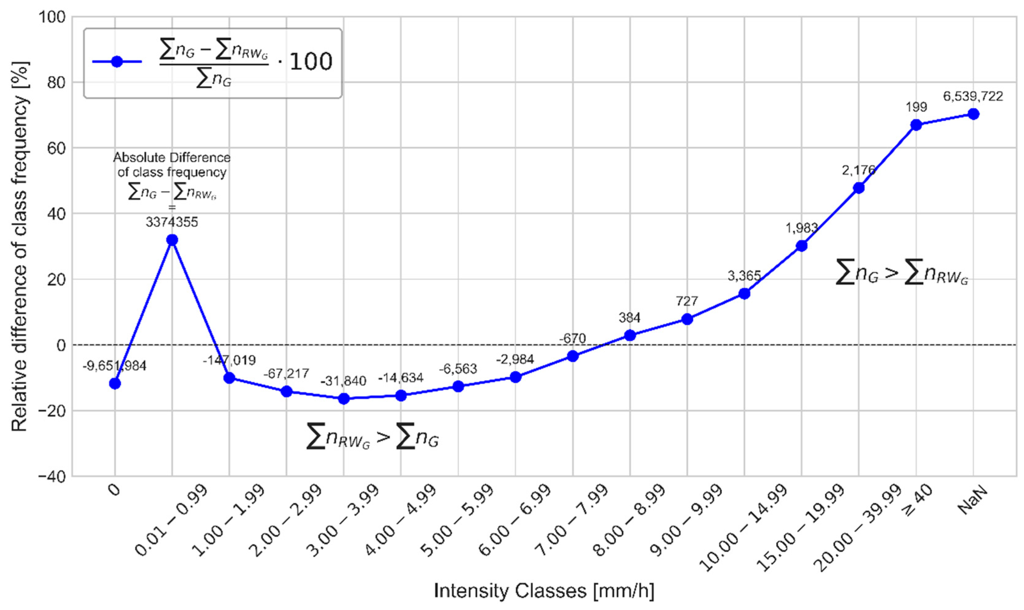
3.4. Rainfall Detection Rates, Heavy Rainfall Days and Rainfall Intensities

In the summer half-year, RADKLIM and RADOLAN detected more days with rainfall > 1 mm than in winter, whereas the gauge dataset showed very little difference between seasons in terms of count and average precipitation (see Figure 9, left). In RADKLIM, however, the mean precipitation per rainy day is almost 40% higher in summer than in winter, which, again, indicates an underestimation of winter precipitation. RADOLAN showed the highest count in both seasons but by far the lowest precipitation average, especially in summer. On the one hand, this is due to the clutter in the first years of the time series, which are characterized by frequent weak radar echoes caused by, for example, wind energy plants, that are converted into many intervals with very weak precipitation. On the other hand, the count of rainfall days is influenced by the unequal completeness of the time series. While RADOLAN has very few NoData intervals due to the filling of gaps with interpolated data, RADKLIM has the clearly outlined gaps caused by the reduction of the radar radius. The gauge dataset suffers additionally from a relatively incomplete time series due to frequent changes in the gauge network. For a more detailed discussion of the reasons for the much higher number of missing data in the rain gauge dataset, which becomes apparent in Figure 10, please refer to [47].
The analysis of heavy rainfall days (see Figure 9, right) showed, as expected, much higher counts in the summer half-year, during which more small-scale convective heavy rainfall events add to large-scale frontal systems that occur throughout the entire year. More surprisingly, the mean precipitation per heavy rainfall day is largely similar between all datasets as well as between seasons. However, despite the almost identical average precipitation in summer and the lower NoData count, RADKLIM counted fewer heavy rainfall days than the gauge dataset. This can be partly explained by the distribution of hourly rainfall intensities (see Figure 10) and the related differences in spatial scale of both measurement methods. In the intensity classes between 1 and 8 mm, more intervals were recorded in RADKLIM than in the gauge dataset. On the one hand, chances are higher that rainfall occurs anywhere within the air column above the 1 km2 area of the radar pixel than within the 200 cm2 small opening of the gauge. On the other hand, this is a logical consequence of the higher NaN count of the gauges, which lack rainfall intervals in return. The divergent ratio for the lowest class < 1 mm can most likely be attributed to an erroneous filtering of low reflectivities during clutter correction and to a shading of light precipitation, e.g., behind other rainfall cells. However, in the classes ≥ 8 mm, the gauges contained more intervals and there was a constantly increasing difference between the datasets.
It has to be mentioned that, despite careful data cleaning, the gauge data might still contain several values representing aggregations of longer time periods due to temporary malfunctions of the gauges. This could slightly overemphasize the difference between datasets for the high intensity classes, but the amount of questionable values is too small to bias the overall distribution in a significant way. Instead, the latter results from the difference in measurements scales and methods. While the radar covers a larger area, the final value of the pixel actually represents the average precipitation of the entire 1 km2 pixel area. Consequently, the different spatial measurement scales inevitably cause deviations between the recorded precipitation intensities. The chance to detect precipitation is higher within the radar pixel, but the averaging of the larger area is likely to cause a lower intensity compared to the gauges. In addition, especially for heavy rainfall events, the radar underestimates rainfall intensity due to signal loss behind heavy rainfall cells. According to [27], the underestimation caused by path-integrated rainfall-induced attenuation along the radar beam can reach a factor of three for uncorrected reflectivity during extreme rainfall events, which is hard to correct adequately.

4. Discussion

All three datasets analyzed in this study showed different advantages and disadvantages, but also positive developments throughout the last years. For example, the considerable improvements in the RADOLAN routines, especially in terms of clutter removal, have to be highlighted. An additional improvement is to be expected due to the polarimetric information added to the precipitation estimation procedure since October 2017, which could not be addressed in this study. Dual-polarised Doppler radar systems allow a better distinction between meteorological and non-meteorological signals (e.g., insects, birds, airplanes, buildings, terrain) and help to classify different hydrometeor types such as raindrops, hail and snow [21,54]. On the one hand, since RADOLAN is an operational QPE product for which time series consistency is not a primary issue, it allows a steady implementation of new technologies and research results. On the other hand, features such as the attenuation correction and additional disaggregated gauge data for adjustment, which require long-term observations and need to be applied retrospectively, cannot be implemented into the RADOLAN routines. Consequently, for operational applications related to heavy rainfall and flood monitoring, precipitation nowcasting, and also as input data for Numerical Weather Prediction, which all require spatially highly resolved, near real-time information, the latest RADOLAN data are undoubtedly a good choice. Still, a certain underestimation of precipitation quantity has to be taken into account when using recent RADOLAN data. However, RADOLAN is not suited for climatological applications and aggregated precipitation statistics, due to the very inconsistent time series and the extreme uncertainties in quantitative precipitation estimations in the first years of the time series.
RADKLIM has been developed in order to provide a longer and largely consistent time series next to the operational data, which can, in return, not profit to the same extent as RADOLAN from recent technological developments since the Dual-Pol information is not available for large portions of the time series. The most striking result concerning RADKLIM’s data quality is the universal underestimation of precipitation, which is evident at all analyzed temporal scales. RADKLIM underestimates the mean annual precipitation sum by about 7.9% (9.1% for gauge-pixel pairs) compared to the gauges and shows fewer hourly intervals of high intensity than the gauge dataset. Only about 0.3 percentage points of the MAP underestimation can be attributed to the radar gaps due to the reduced radius, so that there is quite a systematic negative bias in the data. Most other studies on radar-based QPE evaluations also revealed underestimations of precipitation totals [9,55,56,57,58], but a few authors reported an overestimation [56,59]. However, such results are hard to compare due to large differences in radar hardware, correction algorithms and evaluation methods in the studies. Still, the observed underestimation is rather surprising since a lot emphasis was laid on the correction of attenuation and spokes during the development of RADKLIM, which should, in theory, reduce underestimation and increase precipitation sums. Regarding attenuation, spokes and orographic precipitation, our analyses showed significant improvements, which should indicate an increase in precipitation depth. Nevertheless, the RADKLIM MAP is considerably lower than the RADOLAN MAP throughout the entire study period and the RADKLIM/RADOLAN ratio (see Figure 6) revealed that RADKLIM suffers from an almost ubiquitous negative bias, which is particularly pronounced at close range from the radar. Supported by the very low number of RADKLIM intervals between 0.1 and 1 mm/h (see Figure 10), these findings suggest that low reflectivity signals might be overcorrected and, hence, light rainfall is likely to be suppressed by the RADKLIM routines. In addition, high intensity rainfall is also underestimated, most likely due to the averaging of the pixel area and path-integrated rainfall-induced attenuation. The latter effect is very hard to account for sufficiently during reanalysis because it varies strongly in space and time. As a consequence, the RADKLIM data show many improvements concerning typical radar-related errors, but in return, new errors were induced that offset the positive developments at least to some degree. Regarding the degree of underestimation, however, it has to be noted that, especially with a higher prevalence of snow, the weighing gauge type used by DWD also tends to underestimate precipitation sums due to wind drift [60,61]. Taking this into account, the underestimation of the actual precipitation by the radar products is most likely to be even higher than shown in the analyses.
Depending on the application the radar data is intended to be used for, the underestimation may need to be corrected. For erosion modelling, Fischer et al. [33] already suggested correction factors to account for different methods and spatiotemporal scales. More research on this topic and evaluation studies will be needed in order to further increase the usability of radar data and the reliability and transferability of such correction approaches.
An additional distortion and challenge for the usage of the German radar products arises from the custom polar-stereographic projection, which is used for the datasets. This custom projection is equal of angle while focusing on the North Pole, which is quite unusual for the spatial representation of Germany. Problems occur, when radar composite data are combined with geodata in official projections in GIS such as Digital Elevation Models (DEM) or land use data. Official coordinate systems, like ETRS89, UTM or Gauss–Krüger, are based on a transverse Mercator projection with a Cartesian coordinate grid. Transformations of polar stereographic radar data into Cartesian grids lead to rectangular cells with raster widths of e.g., 944 m horizontally and 955 m vertically. Blending such outcomes with quadratic raster data, e.g., DEM, leads to unavoidable three-dimensional distortions and loss of information. Comprehensive reprojection of the RADKLIM cells on a vector basis at high spatial resolution, including subsequent assignment of the radar data by zonal statistics, is then required to minimize the loss of value and spatial offset.
Despite the shortcomings and uncertainties discussed above, the high spatiotemporal resolution and nationwide coverage of RADKLIM and RADOLAN are major advantages over the point-scale resolution of gauges, which have a disputable spatial representativity especially for capturing local small-scale precipitation events. On the one hand, this high resolution of the radar datasets comes along with large data volumes and challenges in efficient processing of the proprietary binary data files used by DWD. On the other hand, the uniform, centralized dataset derivation of the radar climatology implies a high spatial and temporal consistency, completeness, reliability and documentation, whereas documentation on the gauge data is very insufficient and metadata are distributed over many different files. Consequently, a proper data quality check to account for erroneous entries in the gauge data becomes a very time-consuming task, which is unspecified in most studies using rain gauge data. Moreover, emerging open source software projects help to overcome the challenge of processing and visualizing the radar composite data [48].
Finally, it has to be noted that the direct comparison of radar and gauge data inevitably leads to discrepancies because of the different measurement methods and scales explained above. Moreover, both radar datasets and the gauge data are not entirely independent since some of the gauges are used for adjustment. Both limitations were accepted by the authors due to a lack of representative alternative data for evaluation. Further, more independent approaches for data evaluation and the impacts of the identified errors could include hydrological rainfall-runoff modelling and validation using discharge measurements. However, modelling also inevitably introduces new uncertainties related to model parameterization and input data resolution and quality [62].

5. Conclusions

In this study, the German radar-based QPE products RADOLAN and RADKLIM were compared and evaluated against rain gauge data in order to assess their inherent bias and errors and to assess their recent developments, differences and potentials. With regard to the research questions posed for this study, the key outcomes can be summarized as follows:
1. The modifications in the radar hardware network as well as changes in the RADOLAN processing routines are clearly visible in the RADOLAN time series and lead to a successive increase in data reliability. Clutter and extreme high outliers could be reduced significantly especially since 2010, whereas the quantification of orographic precipitation and range-dependent attenuation remain major error sources. All in all, this causes a decrease in precipitation totals throughout the rather inconsistent RADOLAN time series.
2. The additional correction algorithms implemented for RADKLIM lead to a much more plausible spatial distribution of precipitation totals compared to RADOLAN. RADKLIM shows much fewer typical radar artefacts, an improved representation of orography with the greatest changes during the winter half-year and an efficient correction of range-dependent path-integrated attenuation at longer time scales. However, the latter improvement comes along with a reduced radar radius, which causes several temporary gaps during hardware updates in the otherwise consistent dataset. Moreover, despite the very positive developments in mapping the spatial precipitation distribution, there is an overall negative bias in the RADKLIM precipitation totals, which might be caused by overcorrection of low reflectivities and an underestimation of high intensity rainfall due to spatial averaging and rainfall-induced attenuation of the radar beam.
3. The high spatiotemporal resolution of the radar QPEs is a crucial advantage over the point-scale rain gauge data. Certainly, the higher resolution and spatial coverage require a more automated and efficient data processing approach, but first software solutions for this have already been developed by the radar user community. Moreover, the good documentation of the radar data and, in the case of RADKLIM also the high degree of consistency regarding hardware and data processing, increase their reliability compared to the sparsely documented gauge data, which require a thorough treatment of data gaps and erroneous values. In order to combine RADKLIM data more easily with official geodata, a projection should be sought that can be transformed into official projection systems, e.g., ETRS89, free of distortion and loss of value. This should be done in the framework of future reanalysis runs by DWD.
Certainly, users need to be aware of the outlined weaknesses of the radar-based QPEs in order to interpret their results properly. However, radar QPE products are the precipitation data with the highest spatiotemporal resolution for Germany. In addition to the high degree of consistency and the time series reaching a length that starts to become eligible for climatological analyses, this makes the radar climatology a very promising dataset for various applications.

Author Contributions

Conceptualization, J.K. and B.T.; methodology, J.K.; software, J.K.; validation, J.K. and B.T.; formal analysis, J.K.; data curation, J.K.; writing—original draft preparation, J.K.; writing—review and editing, B.T., G.K., B.B. and J.K.; visualization, J.K.; supervision, G.K., B.B. and B.T. All authors have read and agreed to the published version of the manuscript.

Funding

This research was partially funded by the Hessian Agency for Nature Conservation, Environment and Geology (HLNUG) within the project “KLIMPRAX–Starkregen”, working package 1.4. The publication of this article was funded by the Open Access Fund of the Leibniz Universität Hannover.

Acknowledgments

The authors are grateful to DWD for providing open access radar and rain gauge data. Thanks to Angie Faust for proofreading and to the three anonymous reviewers for their fast and proficient reviews that helped improve the manuscript.

Conflicts of Interest

The authors declare no conflicts of interest. The funders had no role in the design of the study; in the collection, analyses, or interpretation of data; in the writing of the manuscript, or in the decision to publish the results.

References

  1. Global Climate Observing System (GCOS). The Global Observing System for Climate: Implementation Needs; WMO-Pub GCOS-200; GCOS: Geneva, Switzerland, 2016; Available online: https://unfccc.int/sites/default/files/gcos_ip_10oct2016.pdf (accessed on 14 February 2019).
  2. Kidd, C.; Becker, A.; Huffman, G.J.; Muller, C.L.; Joe, P.; Skofronick-Jackson, G.; Kirschbaum, D.B. So, how much of the Earth’s surface is covered by rain gauges? Bull. Am. Meteorol. Soc. 2017, 98, 69–78. [Google Scholar] [CrossRef] [PubMed]
  3. Lochbihler, K.; Lenderink, G.; Siebesma, A.P. The spatial extent of rainfall events and its relation to precipitation scaling. Geophys. Res. Lett. 2017, 44, 8629–8636. [Google Scholar] [CrossRef]
  4. Sun, X.; Mein, R.G.; Keenan, T.D.; Elliott, J.F. Flood estimation using radar and raingauge data. J. Hydrol. 2000, 239, 4–18. [Google Scholar] [CrossRef]
  5. Thorndahl, S.; Einfalt, T.; Willems, P.; Nielsen, J.E.; ten Veldhuis, M.-C.; Arnbjerg-Nielsen, K.; Rasmussen, M.R.; Molnar, P. Weather radar rainfall data in urban hydrology. Hydrol. Earth Syst. Sci. 2017, 21, 1359–1380. [Google Scholar] [CrossRef] [Green Version]
  6. Villarini, G.; Mandapaka, P.V.; Krajewski, W.F.; Moore, R.J. Rainfall and sampling uncertainties: A rain gauge perspective. J. Geophys. Res. 2008, 113. [Google Scholar] [CrossRef]
  7. Abon, C.C.; Kneis, D.; Crisologo, I.; Bronstert, A.; David, C.P.C.; Heistermann, M. Evaluating the potential of radar-based rainfall estimates for streamflow and flood simulations in the Philippines. Geomat. Nat. Hazards Risk 2015, 7, 1390–1405. [Google Scholar] [CrossRef]
  8. Cole, S.J.; Moore, R.J. Hydrological modelling using raingauge- and radar-based estimators of areal rainfall. J. Hydrol. 2008, 358, 159–181. [Google Scholar] [CrossRef]
  9. Hazenberg, P.; Leijnse, H.; Uijlenhoet, R. Radar rainfall estimation of stratiform winter precipitation in the Belgian Ardennes. Water Resour. Res. 2011, 47, 257. [Google Scholar] [CrossRef]
  10. Jessen, M.; Einfalt, T.; Stoffer, A.; Mehlig, B. Analysis of heavy rainfall events in North Rhine–Westphalia with radar and raingauge data. Atmos. Res. 2005, 77, 337–346. [Google Scholar] [CrossRef]
  11. Kitchen, M.; Blackall, R.M. Representativeness errors in comparisons between radar and gauge measurements of rainfall. J. Hydrol. 1992, 134, 13–33. [Google Scholar] [CrossRef]
  12. Meißner, D.; Gebauer, S.; Schumann, A.H.; Pahlow, M.; Rademacher, S. Analyse radarbasierter Niederschlagsprodukte als Eingangsdaten verkehrsbezogener Wasserstandsvorhersagen am Rhein. Hydrol. Und Wasserbewirtsch. Hywa 2012, 56, 16–28. [Google Scholar]
  13. Seo, B.-C.; Krajewski, W.F. Scale Dependence of Radar Rainfall Uncertainty: Initial Evaluation of NEXRAD’s New Super-Resolution Data for Hydrologic Applications. J. Hydrometeor 2010, 11, 1191–1198. [Google Scholar] [CrossRef]
  14. Satgé, F.; Ruelland, D.; Bonnet, M.-P.; Molina, J.; Pillco, R. Consistency of satellite-based precipitation products in space and over time compared with gauge observations and snow- hydrological modelling in the Lake Titicaca region. Hydrol. Earth Syst. Sci. 2019, 23, 595–619. [Google Scholar] [CrossRef] [Green Version]
  15. Crisologo, I.; Warren, R.; Mühlbauer, K.; Heistermann, M. Enhancing the consistency of spaceborne and ground-based radar comparisons by using quality filters. Atmos. Meas. Tech. Discuss. 2018, 1–20. [Google Scholar] [CrossRef]
  16. Ramsauer, T.; Weiß, T.; Marzahn, P. Comparison of the GPM IMERG Final Precipitation Product to RADOLAN Weather Radar Data over the Topographically and Climatically Diverse Germany. Remote Sens. 2018, 10, 2029. [Google Scholar] [CrossRef] [Green Version]
  17. Pejcic, V.; Tromel, S.; Muhlbauer, K.; Saavedra, P.; Beer, J.; Simmer, C. Synergy of GPM and ground-based radar observations for precipitation estimation and detection of microphysical processes. Int. Radar Symp. 2018, 1–8. [Google Scholar]
  18. Pejcic, V.; Saavedra Garfias, P.; Mühlbauer, K.; Troemel, S.; Simmer, C. Evaluation of Germany’s network radar Composite Rain Producs with GPM Near Surface Precipitation Estimations; Earth and Space Science Open Archive: San Francisco, CA, USA, 2019. [Google Scholar]
  19. Gilewski, P.; Nawalany, M. Inter-Comparison of Rain-Gauge, Radar, and Satellite (IMERG GPM) Precipitation Estimates Performance for Rainfall-Runoff Modeling in a Mountainous Catchment in Poland. Water 2018, 10, 1665. [Google Scholar] [CrossRef] [Green Version]
  20. Kidd, C.; Bauer, P.; Turk, J.; Huffman, G.J.; Joyce, R.; Hsu, K.-L.; Braithwaite, D. Intercomparison of High-Resolution Precipitation Products over Northwest Europe. J. Hydrometeor 2012, 13, 67–83. [Google Scholar] [CrossRef] [Green Version]
  21. Berne, A.; Krajewski, W.F. Radar for hydrology: Unfulfilled promise or unrecognized potential? Adv. Water Resour. 2013, 51, 357–366. [Google Scholar] [CrossRef]
  22. Kidd, C.; Levizzani, V. Status of satellite precipitation retrievals. Hydrol. Earth Syst. Sci. 2011, 15, 1109–1116. [Google Scholar] [CrossRef] [Green Version]
  23. Keupp, L.; Winterrath, T.; Hollmann, R. Use of Weather Radar Data for Climate Data Records in WMO Regions IV and VI; WMO: Geneva, Switzerland, 2017. [Google Scholar]
  24. Overeem, A.; Holleman, I.; Buishand, A. Derivation of a 10-Year Radar-Based Climatology of Rainfall. J. Appl. Meteor. Climatol. 2009, 48, 1448–1463. [Google Scholar] [CrossRef]
  25. Bartels, H.; Weigl, E.; Reich, T.; Lang, W.; Wagner, A.; Kohler, O.; Gerlach, N. MeteoSolutions GmbH: Projekt RADOLAN—Routineverfahren zur Online-Aneichung der Radarniederschlagsdaten Mit Hilfe Von Automatischen Bodenniederschlagsstationen (Ombrometer); Zusammenfassender Abschlussbericht für die Projektlaufzeit von 1997 bis 2004; DWD: Offenbach, Germany, 2004. [Google Scholar]
  26. Hänsel, P.; Kaiser, A.; Buchholz, A.; Böttcher, F.; Langel, S.; Schmidt, J.; Schindewolf, M. Mud Flow Reconstruction by Means of Physical Erosion Modeling, High-Resolution Radar-Based Precipitation Data, and UAV Monitoring. Geosciences 2018, 8, 427. [Google Scholar] [CrossRef] [Green Version]
  27. Bronstert, A.; Agarwal, A.; Boessenkool, B.; Crisologo, I.; Fischer, M.; Heistermann, M.; Köhn-Reich, L.; López-Tarazón, J.A.; Moran, T.; Ozturk, U.; et al. Forensic hydro-meteorological analysis of an extreme flash flood: The 2016-05-29 event in Braunsbach, SW Germany. Sci. Total Environ. 2018, 977–991. [Google Scholar] [CrossRef] [PubMed]
  28. Johann, G.; Ott, B.; Treis, A. Einfluss von terrestrisch gemessenen und radarbasierten Niederschlagsdaten auf die Qualität der Hochwasservorhersage. Korresp. Wasserwirtsch. 2009, 9, 487–493. [Google Scholar]
  29. Fischer, F.; Hauck, J.; Brandhuber, R.; Weigl, E.; Maier, H.; Auerswald, K. Spatio-temporal variability of erosivity estimated from highly resolved and adjusted radar rain data (RADOLAN). Agric. For. Meteorol. 2016, 223, 72–80. [Google Scholar] [CrossRef]
  30. Fischer, F.K.; Kistler, M.; Brandhuber, R.; Maier, H.; Treisch, M.; Auerswald, K. Validation of official erosion modelling based on high-resolution radar rain data by aerial photo erosion classification. Earth Surf. Process. Landf. 2018, 43, 187–194. [Google Scholar] [CrossRef]
  31. Winterrath, T.; Brendel, C.; Junghänel, T.; Klameth, A.; Lengfeld, K.; Walawender, E.; Weigl, E.; Hafer, M.; Becker, A. An overview of the new radar-based precipitation climatology of the Deutscher Wetterdienst—Data, methods, products. In Proceedings of the UrbanRain18, 11th International Workshop on Precipitation in Urban Areas, Urban Areas, Zürich, Switzerland, 5–7 December 2018. [Google Scholar]
  32. Lengfeld, K.; Winterrath, T.; Junghänel, T.; Becker, A. Characteristic spatial extent of rain events in Germany from a radar-based precipitation climatology. In Proceedings of the UrbanRain18, 11th International Workshop on Precipitation in Urban Areas, Urban Areas, Zürich, Switzerland, 5–7 December 2018. [Google Scholar]
  33. Fischer, F.K.; Winterrath, T.; Auerswald, K. Temporal- and spatial-scale and positional effects on rain erosivity derived from point-scale and contiguous rain data. Hydrol. Earth Syst. Sci. 2018, 22, 6505–6518. [Google Scholar] [CrossRef] [Green Version]
  34. Auerswald, K.; Fischer, F.K.; Winterrath, T.; Brandhuber, R. Rain erosivity map for Germany derived from contiguous radar rain data. Hydrol. Earth Syst. Sci. 2019, 23, 1819–1832. [Google Scholar] [CrossRef] [Green Version]
  35. Deutscher Wetterdienst Open Data Portal. Historische Stündliche RADOLAN-Raster der Niederschlagshöhe (Binär). Available online: https://opendata.dwd.de/climate_environment/CDC/grids_germany/hourly/radolan/historical/bin/ (accessed on 7 October 2019).
  36. Weigl, E. RADOLAN Information Nr. 13. Available online: https://www.dwd.de/DE/leistungen/radolan/radolan_info/radolan_info_nr_13.pdf?__blob=publicationFile&v=3 (accessed on 8 October 2019).
  37. Weigl, E. RADOLAN Information Nr. 15. Available online: https://www.dwd.de/DE/leistungen/radolan/radolan_info/radolan_info_nr_15.pdf?__blob=publicationFile&v=3 (accessed on 8 October 2019).
  38. Weigl, E.; Winterrath, T. Radargestützte Niederschlagsanalyse und—Vorhersage (RADOLAN, RADVOR-OP). Promet 2009, 35, 78–86. [Google Scholar]
  39. Weigl, E. RADOLAN-Information Nr. 17. Available online: https://www.dwd.de/DE/leistungen/radolan/radolan_info/radolan_info_nr_17.pdf?__blob=publicationFile&v=3 (accessed on 17 June 2019).
  40. Stephan, K. Erfahrungsbericht zur Verwendung des PULL-Kompositverfahrens zur Erstellung des Radolan-Komposits (RZ-Komposit). 2007; Unpublished work. [Google Scholar]
  41. Weigl, E. RADOLAN-Information Nr. 41. Available online: https://www.dwd.de/DE/leistungen/radolan/radolan_info/radolan_info_nr_41.pdf;jsessionid=65C71E4F45253E6B3CE3F24F443D3E2B.live11044?__blob=publicationFile&v=2 (accessed on 17 December 2019).
  42. Weigl, E. RADOLAN-Information Nr. 45. Available online: https://www.dwd.de/DE/leistungen/radolan/radolan_info/radolan_info_nr_45.pdf;jsessionid=65C71E4F45253E6B3CE3F24F443D3E2B.live11044?__blob=publicationFile&v=3 (accessed on 17 December 2019).
  43. Winterrath, T.; Brendel, C.; Hafer, M.; Junghänel, T.; Klameth, A.; Lengfeld, K.; Walawender, E.; Weigl, E.; Becker, A. Radar Climatology (RADKLIM) Version 2017.002 (RW). Gridded Precipitation Data for Germany; Available online: https://opendata.dwd.de/climate_environment/CDC/grids_germany/hourly/radolan/reproc/2017_002/bin (accessed on 25 June 2019).
  44. Winterrath, T.; Brendel, C.; Hafer, M.; Junghänel, T.; Klameth, A.; Lengfeld, K.; Walawender, E.; Weigl, E.; Becker, A. Radar Climatology (RADKLIM) Version 2017.002 (YW). Gridded Precipitation Data for Germany; Available online: https://opendata.dwd.de/climate_environment/CDC/grids_germany/5_minutes/radolan/reproc/2017_002/bin/ (accessed on 25 June 2019).
  45. Winterrath, T.; Brendel, C.; Hafer, M.; Junghänel, T.; Klameth, A.; Walawender, E.; Weigl, E.; Becker, A. Erstellung Einer Radargestützten Niederschlagsklimatologie. Berichte des Deutschen Wetterdienstes No. 251; 2017; Available online: https://www.dwd.de/DE/leistungen/pbfb_verlag_berichte/pdf_einzelbaende/251_pdf.pdf?__blob=publicationFile&v=2 (accessed on 29 March 2019).
  46. Deutscher Wetterdienst Open Data Portal. Rain Gauge Precipitation Observations in 1-Minute Resolution. Available online: https://opendata.dwd.de/climate_environment/CDC/observations_germany/climate/1_minute/precipitation/ (accessed on 10 January 2019).
  47. Kreklow, J.; Tetzlaff, B.; Kuhnt, G.; Burkhard, B. A Rainfall Data Intercomparison Dataset of RADKLIM, RADOLAN, and Rain Gauge Data for Germany. Data 2019, 4, 118. [Google Scholar] [CrossRef] [Green Version]
  48. Kreklow, J. Facilitating radar precipitation data processing, assessment and analysis: A GIS-compatible python approach. J. Hydroinformatics 2019, 21, 652–670. [Google Scholar] [CrossRef] [Green Version]
  49. Kreklow, J. Radproc—A Gis-Compatible Python-Package for Automated Radolan Composite Processing and Analysis; Zenodo: Geneva, Switzerland, 2018; Available online: https://zenodo.org/record/2539441 (accessed on 25 June 2019).
  50. Kreklow, J.; Tetzlaff, B.; Kuhnt, G.; Burkhard, B. A Rainfall Data Inter-Comparison Dataset for Germany: Version 1.0; Zenodo: Geneva, Switzerland, 2019; Available online: https://zenodo.org/record/3262172 (accessed on 29 June 2019).
  51. Tukey, J. Exploratory Data Analysis; Addison-Wesley: Boston, MA, USA, 1977. [Google Scholar]
  52. Deutscher Wetterdienst. Jahresrückblick 2007 des Deutschen Wetterdienstes. Gefährliche Wetterereignisse Und Wetterschäden in Deutschland; Offenbach am Main: Offenbach, Germany, 2007. [Google Scholar]
  53. Deutscher Wetterdienst. Jahresbericht 2016. 2017. Available online: https://www.dwd.de/DE/leistungen/jahresberichte_dwd/jahresberichte_pdf/jahresbericht_2016.pdf?__blob=publicationFile&v=3 (accessed on 18 December 2019).
  54. Grazioli, J.; Tuia, D.; Berne, A. Hydrometeor classification from polarimetric radar measurements: A clustering approach. Atmos. Meas. Tech. 2015, 8, 149–170. [Google Scholar] [CrossRef] [Green Version]
  55. Goudenhoofdt, E.; Delobbe, L. Generation and Verification of Rainfall Estimates from 10-Yr Volumetric Weather Radar Measurements. J. Hydrometeor 2016, 17, 1223–1242. [Google Scholar] [CrossRef]
  56. Fairman, J.G.; Schultz, D.M.; Kirshbaum, D.J.; Gray, S.L.; Barrett, A.I. A radar-based rainfall climatology of Great Britain and Ireland. Weather 2015, 70, 153–158. [Google Scholar] [CrossRef] [Green Version]
  57. Smith, J.A.; Baeck, M.L.; Villarini, G.; Welty, C.; Miller, A.J.; Krajewski, W.F. Analyses of a long-term, high-resolution radar rainfall data set for the Baltimore metropolitan region. Water Resour. Res. 2012, 48, 616. [Google Scholar] [CrossRef]
  58. Schleiss, M.; Olsson, J.; Berg, P.; Niemi, T.; Kokkonen, T.; Thorndahl, S.; Nielsen, R.; Nielsen, J.E.; Bozhinova, D.; Pulkkinen, S. The Accuracy of Weather Radar in Heavy Rain: A Comparative study for Denmark, the Netherlands, Finland and Sweden. Hydrol. Earth Syst. Sci. Discuss. 2019, 1–42. [Google Scholar] [CrossRef] [Green Version]
  59. Marra, F.; Morin, E. Use of radar QPE for the derivation of Intensity–Duration–Frequency curves in a range of climatic regimes. J. Hydrol. 2015, 531, 427–440. [Google Scholar] [CrossRef]
  60. Boudala, F.S.; Isaac, G.A.; Filman, P.; Crawford, R.; Hudak, D.; Anderson, M. Performance of Emerging Technologies for Measuring Solid and Liquid Precipitation in Cold Climate as Compared to the Traditional Manual Gauges. J. Atmos. Ocean. Technol. 2017, 34, 167–185. [Google Scholar] [CrossRef]
  61. Kochendorfer, J.; Rasmussen, R.; Wolff, M.; Baker, B.; Hall, M.E.; Meyers, T.; Landolt, S.; Jachcik, A.; Isaksen, K.; Brækkan, R.; et al. The quantification and correction of wind-induced precipitation measurement errors. Hydrol. Earth Syst. Sci. 2017, 21, 1973–1989. [Google Scholar] [CrossRef] [Green Version]
  62. Heistermann, M.; Kneis, D. Benchmarking quantitative precipitation estimation by conceptual rainfall-runoff modeling. Water Resour. Res. 2011, 47, 301. [Google Scholar] [CrossRef] [Green Version]
Figure 1. Height above sea level (m) of Germany based on a SRTM Digital Elevation Model (left map) and German radar station network with 128 km radius as used for RADKLIM (right map).
Atmosphere 11 00217 g001
Figure 2. Spatiotemporal distribution of outliers in the annual precipitation sums of RADOLAN and RADKLIM. Blue values represent high outliers (MAP > cleaned MAP), yellow and red values represent low outliers (cleaned MAP > MAP).
Atmosphere 11 00217 g002
Figure 3. Mean annual precipitation sums for the period 2006 to 2017 derived from (a) RADKLIM, (b) RADOLAN and (c) gauge data.
Atmosphere 11 00217 g003
Figure 4. Mean annual precipitation sums of Germany between 2006–2017.
Atmosphere 11 00217 g004
Figure 5. Comparison of mean annual precipitation sums from the 997 rain gauges and the corresponding RADKLIM pixels (left plot) as well as from the 392529 RADOLAN-RADKLIM pixel pairs (right plot).
Atmosphere 11 00217 g005
Figure 6. Ratio of mean annual and seasonal precipitation sums 2006–2017 between RADKLIM and RADOLAN.
Atmosphere 11 00217 g006
Figure 7. Quadratic regression between seasonal precipitation sums and altitude for gauges (left plot), RADKLIM (centre) and RADOLAN (right).
Atmosphere 11 00217 g007
Figure 8. Linear regression between the distance from the next radar and the RADKLIM/gauge MAP ratio (left plot) as well as the RADOLAN/gauge MAP ratio (right plot).
Atmosphere 11 00217 g008
Figure 9. Number of days with precipitation amounts >1 mm (left plot) and >20 mm (right plot) in summer and winter half-years for gauges, RADKLIM and RADOLAN data. The numbers above the bars indicate the average daily precipitation sum of all days exceeding the respective threshold.
Atmosphere 11 00217 g009
Figure 10. Difference of intensity class frequency between all point-pixel data pairs (n = 997) of the period 2006–2017 of gauge data ( n G ) and RADKLIM RW product ( n R W G ).
Atmosphere 11 00217 g010
Table 1. Overview of the final RADKLIM and RADOLAN composite datasets.
Radar ProductOpen AccessTime PeriodTemporal Resolution [min]Radar Radius [km]National Grid [km]
RADKLIM RWYes2001–2018601281100 × 900
RADKLIM YWYes2001–201851281100 × 900
RADOLAN RWYesSince June 200560125/150900 × 900
RADOLAN RYNoSince June 20055125/150900 × 900

