Article

A Four Dimensional Variational Data Assimilation Framework for Wind Energy Potential Estimation

by
Elias D. Nino-Ruiz
1,*,†,
Juan C. Calabria-Sarmiento
1,2,†,
Luis G. Guzman-Reyes
1,† and
Alvin Henao
3,†
1
Applied Math and Computer Science Laboratory, Department of Computer Science, Universidad del Norte, Barranquilla 080001, Colombia
2
Department of Computer Science, Universidad Simon Bolivar, Barranquilla 080001, Colombia
3
Industrial Engineering Department, Universidad del Norte, Barranquilla 080001, Colombia
*
Author to whom correspondence should be addressed.
These authors contributed equally to this work.
Atmosphere 2020, 11(2), 167; https://doi.org/10.3390/atmos11020167
Submission received: 6 November 2019 / Revised: 20 December 2019 / Accepted: 2 January 2020 / Published: 5 February 2020
(This article belongs to the Special Issue Climate Modeling for Renewable Energy Resource Assessment)

Abstract

:
In this paper, we propose a Four-Dimensional Variational (4D-Var) data assimilation framework for wind energy potential estimation. The framework is defined as follows: we choose a numerical model which can provide forecasts of wind speeds then, an ensemble of model realizations is employed to build control spaces at observation steps via a modified Cholesky decomposition. These control spaces are utilized to estimate initial analysis increments and to avoid the intrinsic use of adjoint models in the 4D-Var context. The initial analysis increments are mapped back onto the model domain from which we obtain an estimate of the initial analysis ensemble. This ensemble is propagated in time to approximate the optimal analysis trajectory. Wind components are post-processed to get wind speeds and to estimate wind energy capacities. A matrix-free analysis step is derived from avoiding the direct inversion of covariance matrices during assimilation cycles. Numerical simulations are employed to illustrate how our proposed framework can be employed in operational scenarios. A catalogue of twelve Wind Turbine Generators (WTGs) is utilized during the experiments. The results reveal that our proposed framework can properly estimate wind energy potential capacities for all wind turbines within reasonable accuracies (in terms of Root-Mean-Square-Error) and even more, these estimations are better than those of traditional 4D-Var ensemble-based methods. Moreover, large variability (variance of standard deviations) of errors are evidenced in forecasts of wind turbines with the largest rate-capacity while homogeneous variability can be seen in wind turbines with the lowest rate-capacity.

1. Introduction

Data Assimilation (DA) is the process by which an imperfect numerical forecast { x k b } k = 0 G is adjusted according to real noisy observations { y k } k = 0 G [1,2], where x k b R n × 1 and y k R m × 1 are the background state and the observations at step k, for 0 k G , respectively, n is the model size (model resolution), m denotes the number of observations per assimilation step, and G is the size of the assimilation window (the number of times wherein observations are available). In strong constraint Four-Dimensional Variational (4D-Var) methods, cost functions of the form [3,4]:
J x 0 = 1 2 · x 0 x 0 b B 0 1 2 + 1 2 · k = 0 G y k H x k R k 1 2 ,
are employed to perform the assimilation process, where B 0 R n × n and R k R m × m are the covariance matrix of the initial background errors and the estimated data error covariance matrix at step k, respectively. Likewise,
x f = M t f 1 t f x f 1 , for 1 f G ,
where M : R n × 1 R n × 1 is a numerical model which, for instance, mimics the behavior of the ocean and/or the atmosphere and even more, we assume that the model can predict wind components (or wind speeds). We then seek the initial condition which best fit the data:
x 0 a = arg min x 0 J ( x 0 ) , subject to ( 2 ) .
To solve the optimization problem (3), for instance, we can make use of adjoint models (i.e., transpose of linearization of the numerical model) or an ensemble of model realizations. Regardless of which one is chosen, the initial condition (3) can provide a forecast of relevant physical variables (depending on the numerical model) such as wind components, temperature, and humidity. Forecasts of wind components can be exploited in the context of Wind Turbine Generators (WTGs) to estimate the potential energy capacities of wind turbines and then to employ green sources of energy in cities, countries, and even more, remote places wherein these are the unique option. Hence, we can make use of numerical models and 4D-Var optimization problems to estimate wind components (in particular, wind speeds since they are key inputs to size WTG), then by using parameters from wind turbines such as cut-in speed, cut-out speed, and rated wind speed, we can estimate their potential wind power capacity for a specific place. WTG parameters allow choosing the best WTG for a specific place according to its wind-speed values. This can be exploited in places such as the Latin American and the Caribbean (LAC) countries since these are widely known for their large power generation capacity using renewable energies. This makes them highly attractive for clean energy investment [5]. Recent studies indicate that the full deployment of this capacity can be almost seven times larger than the current world installed one, and even more, it can constitute a near-zero carbon emissions option for developing countries [6]. This could provide substantial societal benefits, including energy security, local and global environmental benefits, domestic job creation, and improved balance of payments, amongst others [7]. Given LAC geography, wind turbines (wind farms) can be exploited as clean energy sources. The economic benefits of wind farms are better than those of traditional sources such as solar farms, which make the first option desirable for long-term plans at national levels. The proper planning and scheduling of wind power systems can lead to almost no impact on LAC ecosystems, neither visual or audible. Besides, this can serve as a complement of the hydro-dominated electricity grids [8], as the winds are stronger during the dry season when hydroelectric generation is most limited. Moreover, wind farms can provide a full or complementary source of energy in some areas of difficult access; the application of wind turbines is primarily in windmills that are used to generate electricity [9]. These wind turbines can be used to avail off-grid electricity in remote regions (i.e., some islands).
The structure of this paper is as follows: Section 2 discusses DA formulations and wind turbine generators (WTG). In Section 3, we propose a novel framework for electrical power estimation via WTGs and 4D-Var ensemble DA. In Section 4, numerical simulations are employed to show how our framework can be employed; we generate synthetic scenarios by using an Atmospheric General Circulation Model. Lastly, Section 5 states the conclusions of this research.

2. Preliminaries

In this section, we briefly discuss concepts related to 4D-Var ensemble DA and wind turbine generators. We primarily focus on the necessary topics for the derivation of our 4D-Var ensemble-based method.

2.1. Data Assimilation

To solve the optimization problem (3), we can employ adjoint models to approximate gradients and to condunct optimization steps via, for instance, line-search or trust region methods. However, these models can be labor-intensive to develop and computationally expensive to run. For instance, the adjoint model of the High Resolution Limited Area Modelling (HIRLAM) 4D-Var [10,11] was developed in 10 years in which most of the time was spent to detect and to fix errors in the tangent and the adjoint models [12]. To avoid the use of adjoint models, we can employ an ensemble of model realizations [13] as follows [14,15]:
X k b = x k b [ 1 ] , x k b [ 2 ] , , x k b [ N ] R n × N
where x k b [ e ] R n × 1 stands for the e-th ensemble member, for 1 e N , at time k, for 0 k G . Then, the ensemble mean:
x ¯ k b = 1 N · e = 1 N x k b [ e ] R n × 1 ,
and the ensemble covariance matrix:
P k b = 1 N 1 · Δ X k b · Δ X k b T R n × n ,
act as estimates of the forecast state x k b and the forecast error covariance matrix B k , respectively, where the matrix of member deviations reads:
Δ X k b = X k b x ¯ k b · 1 T R n × N .
The model trajectory in (1) can be constrained to the space spanned by the background ensemble members (4a), this is:
x k = x ¯ k b + Δ X k · w ,
where w R N × 1 is a vector in redundant coordinates to be determined later. This is equivalent to:
x k x ¯ k b range Δ X k range B k 1 / 2 ,
therefore, the estimation of analysis increments is performed onto the sub-space given by a low-rank square root approximation of the background error covariance matrices (4c) at observation times (times where observations are available). By replacing (5) into the Equation (1) one obtains [16]:
J ( x 0 ) = J x ¯ 0 b + Δ X 0 · w = J ^ ( w ) = ( N 1 ) 2 · w 2 + 1 2 · k = 0 G d k Q k · w R k 1 2 ,
where d k = y k H k · x ¯ k b R m × 1 is the innovation vector and Q k = H k · Δ X k b R m × N . Note that, this cost function does not rely in the numerical model (2) anymore. The optimal value of the control variable w is then seek:
w * = arg min w J ^ ( w ) .
The gradient of (6) equals:
w J ^ ( w ) = ( N 1 ) · w k = 0 G Q k T · R k 1 · d k Q k · w = ( N 1 ) · I + k = 0 G Q k T · R k 1 · Q k · w k = 0 G Q k T · R k 1 · d k R N × 1 ,
and from here, the optimal weight (7a) can be approximated as follows:
w * = ( N 1 ) · I + k = 0 G Q k T · R k 1 · Q k 1 · k = 0 G Q k T · R k 1 · d k R N × 1 ,
from which the initial analysis state can be estimated:
x ¯ 0 a = x ¯ 0 b + Δ X 0 b · w * .
Since in (5), x k a represents an approximation rather than an exact analysis trajectory, the initial analysis is recovered and then, it is evolved in time by using the numerical model (2) from which we obtain an estimate of the optimal trajectory of (3):
x ¯ f a = M t f 1 t f x ¯ f 1 a , for 1 f G .
Notice, in the 4D-EnKF, all computations are performed onto the ensemble space (5) and therefore, the computational cost of estimating (7d) is linearly bounded regadring n and m [17]:
O N · n · m + N 2 · m .
Readily, posterior ensemble members at the initial time can be estimated via the implicit covariance matrix in (7c):
x ¯ 0 a ( e ) = x ¯ 0 b + Δ X 0 b · w ( e ) , for 1 e N ,
where:
w ( e ) N w * , ( N 1 ) · I + k = 0 G Q k T · R k 1 · Q k 1 .
In practice, model dimensions range in the order of millions while ensemble sizes are constrained by the hundreds and as a direct consequence, undersampling degrades the quality of analysis corrections onto the space spanned by (4d). To counteract the effects of sampling noise, localizations methods are commonly employed [18,19], in practice. For instance, methods such as covariance matrix localization ( B -localization) [20], domain localization, and observation localization ( R -localization) [21,22,23] are employed in operational DA scenarios. Yet another possible choice is to make use of precision matrix estimation. In this context, for instance, the use of the spatial-predecessors concept can be employed to obtain sparse estimators of precision matrices [24]. The predecessors of model component i, from now on Π ( i , δ ) , for 1 i n and a radius of influence δ Z + , are given by the set of components whose labels are lesser than that of the i-th one. Of course, this will depend on the format employed to label components on a numerical grid. In practice, column major and row major format are commonly employed. This idea is exploited in the EnKF formulation proposed in [25,26] wherein the following estimator is employed to approximate precision matrices [27]:
B ^ k 1 = V ^ k T · Γ ^ k 1 · V ^ k R n × n ,
where the Cholesky factor L k R n × n is a lower triangular matrix,
V ^ k i , g = β i , g , k , g P ( i , δ ) 1 , i = g 0 , o t h e r w i s e ,
whose (sub-diagonal) elements β i , g , k are estimated by fitting linear models:
x [ i ] T k = g Π ( i , δ ) β i , g , k · x [ g ] T k + γ i k R N × 1 , 1 i n ,
where x [ i ] T k R N × 1 denotes the model component i from the ensemble (4a). Likewise, γ i k R N × 1 N 0 , σ 2 · I , where the variance σ k 2 is unknown, and the diagonal matrix Γ k R n × n holds the variance of residuals:
Γ k i , i = var ^ x [ i ] T k g Π ( i , δ ) β i , g , k · x [ j ] T k 1 var γ i k 1 = 1 σ k 2 > 0 , with Γ k 1 , 1 = var ^ x [ 1 ] T k 1 ,
where the empirical and the actual variances are denoted by var ^ ( ) and var ( ) , respectively.

2.2. Wind Energy Potential

The effects of climate change have triggered alarms to employ alternatives and to reduce Carbon Dioxide ( C O 2 ) emissions around the world. In many countries, regulation and C O 2 reduction goals promote the substitution of fossil energy sources with Renewable Energy Sources (RES) [28]. For instance, China, the largest energy consumer worldwide, has an economic motivation to execute such substitution [29]: traditional power systems (mainly composed of nuclear, hydro, and thermal generators) are drastically decreasing, and now, they are trying to integrate RES as a shock absorber of this situation. However, RES integration is not straightforward since it brings new issues and challenges that need to be analyzed and addressed. One of the main challenges comes from the intermittency of RES [30]. Intermittency combines variability and uncertainty. The former is produced by the movement of large cloud systems owing to high and low-pressure areas. Uncertainty, also known as unpredictability, comes from the forecast error, which in turn depends on the numerical model (2). Thus, uncertainty amplification relies on model errors (i.e., physics simplifications to make numerical models computationally feasible to run). For instance, if the accuracy of the numerical model is poor, and no Data Assimilation is performed, the bias on the resulting estimate will be large concerning the actual wind speed. Thus, wind speeds can be poorly estimated, and as a direct consequence, wind energy potentials can be underestimated. Hence, Data Assimilation can be employed in this context to mitigate the impact of poor potential energy estimations via real noisy observations of wind speeds. The potential energy p ( v ) in MegaWatts ( M W ) of a wind turbine given a wind speed v ( k m / h ) can be estimated as follows:
p ( v ) = P n o m · v 3 v c 3 v r 3 v c 3 v c v v r P n o m v r v v f 0 otherwise ,
where v c , v r , v f , and v p are the cut-in wind speed, the rated wind speed, the cut-out wind speed, and the rated power of wind turbine, respectively. Table 1 shows the 12 wind turbine generators types assumed and utilized in many case studies [31]. The outage rate of each wind turbine reads 0.04. Commonly, the useful life of a wind turbine is about 25 years, this does not depend on its size. We also report the capital cost, and the maintenance and operating cost for each turbine, these are taken from [32,33].
Based on the Table 1, places with wind speeds below 10 km/h do not have the chance to generate electrical power from wind speeds since these are lower than the minimum cut-in wind speed across all Wind Turbine Generators (WTGs). Similarly, places with wind speeds greater than 90 km/h cannot produce electrical power because wind speeds exceed the maximum cut-out wind speed (i.e., WTG 6). Although, we do not consider economic impacts of wind-farm placements, it is important to note that wind-speed constraints have economic implications. For instance, for a place with bimodal wind speeds of 40 km/h and 11 km/h, WTGs 1 and 2 can be employed while the rest of them must be discarded in spite of the last are cheaper.

3. Proposed Framework

In this section, we develop an adjoint-free 4D-Var framework for potential energy estimation. The framework is divided into four stages. First, we build an ensemble of snapshots at observation times by employing a numerical model which can forecast wind components. Second, these snapshots are employed to build control spaces via a modified Cholesky decomposition. Third, the control spaces are utilized to obtain initial conditions whose wind forecasts fit a set of time spaced observations. Lastly, forecasts of wind components are employed to estimate forecasts of wind speeds, which in turn allow us to forecast potential energies of Wind Turbine Generators (WTGs). Since, in practice, model resolutions range in the order of the millions, we develop a matrix-free analysis formulation to avoid the direct inversion of linear systems during assimilation steps. All these stages are clearly detailed next.

3.1. Building an Ensemble of Snapshots

Initially, we choose a numerical model which mimics the dynamics of wind components in places of interest. For this purpose, numerical models such as the Atmospheric General Circulation Model (AT-GCM Speedy) [34] and the Weather Research Forecast (WRF) Model [35,36] can be employed. Once the numerical model is chosen, snapshots of an ensemble of model realizations (4a) are taken at G + 1 observation times. At step k, for 0 k G , the background ensemble X k b (4a) is employed to estimate a full-rank square-root approximation of the precision matrix of background errors B k 1 via a modified Cholesky decomposition (8a):
B ^ k 1 / 2 = V ^ k T · Γ ^ k 1 / 2 R n × n .
At this step, we choose a radius of influence (localization radius) δ to compute the factor V ^ k T . Beyond the scope of this radius (and the predecessors of model components) all components of V ^ k T are assumed zero. We exploit the fact that, when the error correlations of two model components are conditionally independent (given a radius of influence δ ), their corresponding entry in the precision matrix of background errors is zero. This results in a sparse Cholesky factor V ^ k T and even more, a localized square-root precision matrix. In this manner, the impact of sampling errors can be mitigated in the square-root approximations (10). Some structures of V ^ k are shown in Figure 1 for a one dimensional grid and different values of δ , cyclic boundary conditions are assumed for physics/dynamics.
The square-root approximations (10) serve as control spaces onto which analysis increments can be estimated, therefore, the analysis increment at observation time k can be written as follows:
x k x ¯ k b range B ^ k 1 / 2 ,
or equivalently:
x k = x ¯ k b + B ^ k 1 / 2 · α R n × 1 ,
where B ^ k 1 / 2 = V ^ k T · Γ ^ k 1 / 2 1 R n × n , and α R n × 1 is a vector in redundant coordinates to be determined later. We assume that:
range V ^ k T · Γ ^ k 1 / 2 1 range B k 1 / 2 .
Note that, since the square root approximations (10) are full-rank, the dimension of the spaces (11) equal those of the range of B 1 / 2 . This differs from what is usually employed in the literature: a control space whose dimension equals the ensemble size (5) and therefore, analysis increments can be highly impacted by sampling noise. We then expect to capture all error dynamics onto the spaces (10).
Since the initial background error covariance matrix B 0 onto the control space (11) is nothing but the identity matrix, the following error statistics hold for the prior weights α b ( e ) :
α b ( e ) N 0 , I , for 1 e N .
Due to this, the 4D-Var cost function (1) onto the control space (11) can be written as follows:
J x 0 = J x ¯ 0 b + B ^ 0 1 / 2 · α = J ˜ α = 1 2 · α 2 + 1 2 · k = 0 G d ˜ k Q ˜ k · α R k 1 2 ,
where d ˜ k = y k H · x ¯ k b R m × 1 , and Q ˜ k = H · B ^ k 1 / 2 R m × n . Again, this cost function does not rely on the numerical model (2).

3.2. Adjoint-Free 4D-Var Optimization

Once the control spaces are estimated across observation times, the adjoint-free optimization problem to solve reads:
α a = arg min α J ˜ α .
The gradient of this cost function can be written as follows:
α J ˜ α = I + k = 0 G Q ˜ k T · R k 1 · Q ˜ k · α k = 0 G Q ˜ k T · R k 1 · d ˜ k ,
whose root reads:
α a = I + k = 0 G Q ˜ k T · R k 1 · Q ˜ k 1 · k = 0 G Q ˜ k T · R k 1 · d ˜ k ,
and therefore an estimate of the initial analysis state (3) can be computed as follows:
x ¯ 0 a = x ¯ 0 b + B ^ 0 1 / 2 · α a ,
whose model trajectory provides a forecast which accounts for the given data into the assimilation window. Note that, the closed form expression (13b) for the optimal weights (13a) is possible since we consider linear observation operators in our formulation. The posterior ensemble onto the control space can then be built by using a square root approximation of the information matrix in (13b), it can be easily shown that the posterior error statistics read:
α a [ e ] N α a , I + k = 0 G Q ˜ k T · R k 1 · Q ˜ k 1 , for 1 e N ,
with corresponding analysis members in the model space:
x 0 a [ e ] = x ¯ b + B ^ 0 1 / 2 · α a [ e ] .
Then, the analysis members of the initial ensemble are propagated in time
x f a [ e ] = M t f 1 t f x f a [ e ] , for 1 f G and 1 e l e N ,
from which an estimate of the optimal trajectory
x k a x ¯ k a = 1 N · e = 1 N x k a [ e ] ,
and his uncertainty (i.e., by employing a modified Cholesky decomposition on the ensemble members at time k) can be obtained. Note that, the posterior mode (13c) can be written as follows:
x ¯ 0 a x ¯ 0 b = B ^ 0 1 / 2 · I + k = 0 G Q ˜ k T · R k 1 · Q ˜ k 1 · k = 0 G Q ˜ k T · R k 1 · d ˜ k ,
which is nothing but a linear transformation of the prior increment to the posterior one. In this sense, the analysis step is similar to that of square root filter formulations. However, we compute the analysis increments of the initial ensemble members by using synthetic data, which is statistically consistent with the posterior error distribution:
x ¯ 0 a [ e ] x ¯ 0 b [ e ] = V ^ T · Γ ^ 1 / 2 · α a + I + k = 0 G Q ˜ k T · R k 1 · Q ˜ k 1 / 2 · ξ [ e ] , with ξ [ e ] N 0 , I .
Readily:
x ¯ 0 a x ¯ 0 b = E 1 N · e = 1 N x ¯ 0 a [ e ] x ¯ 0 b [ e ] ,
and therefore, in spite of the posterior mode of the analysis distribution can be estimated via a linear transformation of the initial background increments, the analysis increments of the initial ensemble are actually computed by employing synthetic data. This places our proposed filter formulation into the family of stochastic formulations of data assimilation methods.
Notice, given the special structure of our estimator B k 1 / 2 , the Woodbury matrix identity can be exploited to avoid direct inversions [37]. We denote this filter implementation Four Dimensional Variational Data Assimilation via a Modified Cholesky Decomposition (4D-Var-MC).

3.3. Post-Processing of Data, Potential Energy Estimation

Once the model trajectory is computed for each ensemble member, we proceed to map wind fields to wind energy potentials in two steps:
  • whenever is necessary, the wind components of ensemble members are mapped to wind-speeds,
  • this subset of information is exploited to estimate the wind energy potential of each analysis ensemble member:
    x ^ k a [ e ] = w x k a [ e ] , for 1 e N , and 0 k G ,
    where w : R n × 1 R h × 1 is a function that maps model states to potential energy states (this is, for each ensemble member, its wind-speed components are mapped to wind energy potentials), where h is the number of wind-speed components (with h n ), and x ^ k a [ e ] R h × 1 is the k-th transformed member. The mapping process depends on the wind turbine employed, for instance, one can consider the wind turbines discussed in Section 2.2.
Note that, the empirical moments of the samples (16) can be exploited to estimate mean and standard deviations of wind energy potential capacities. Besides, covariances of such samples can be estimated via a modified Cholesky decomposition to understand better (and to estimate) their uncertainties.

3.4. Further Comments: Matrix-Free Formulation of the 4D-Var-MC

In practice, the number of model components n range in the order of the millions and therefore, matrix computations can be constrained by computational resources. For instance, the direct inversion of (13b) is prohibitive. Thus, it is mandatory to count with a matrix-free implementation of any data assimilation process. Following the ideas discussed in [38], we can develop a matrix-free equation for the analysis step of the 4D-Var-MC implementation. We can proceed as follows, consider:
Ω = Ω 0 , Ω 1 , , Ω G R n × O
where Ω k = Q ˜ k · R k 1 / 2 R n × m , and O = m · G , the precision matrix in (14) can be written as follows,
A ^ 1 = I + Ω · Ω T = T T · C · T + Ω · Ω T = T T · C · T + o = 1 O · ω [ o ] · ω [ o ] T ,
where ω [ o ] R n × 1 is the o-th column of matrix Ω , for 0 o O , and I = T T · C · T is the Cholesky decomposition of I (all factors equal the identity matrix). Consider the sequence of matrices,
A ^ ( 0 ) = V ( 0 ) T · Γ ( 0 ) · V ( 0 ) = T T · C · T = I , A ^ ( 1 ) = A ^ ( 0 ) + ω [ 1 ] · ω [ 1 ] T = V ( 1 ) T · Γ ( 1 ) · V ( 1 ) , A ^ ( 2 ) = A ^ ( 1 ) + ω [ 2 ] · ω [ 2 ] T = V ( 2 ) T · Γ ( 2 ) · V ( 2 ) , A ^ ( O ) = A ^ ( O 1 ) + ω [ O ] · ω [ O ] T = V ( O ) T · Γ ( O ) · V ( O ) = V ^ T · Γ ^ · V ^ = A ^ 1 ,
where V ( 0 ) R n × n and Γ ( 0 ) R n × n are the factors of the Cholesky decomposition of the identity matrix I . Among iteration steps o, for 0 o O , one can see that:
A ^ ( o ) = V ( o 1 ) T · Γ ( o 1 ) · V ( o 1 ) + ω [ o ] · ω [ o ] T = V ( o 1 ) T · Γ ( o 1 ) + γ ( o ) · γ ( o ) T · V ( o 1 ) ,
where V ( j 1 ) T · γ ( j ) = ω [ j ] R n × 1 . Via the Cholesky factors of,
Γ ( o 1 ) + γ ( o ) · γ ( o ) T = V ˜ ( o 1 ) T · Γ ( o ) · V ˜ ( o 1 ) ,
and, by considering Equation (18), the matrix A ^ ( j ) can be decomposed as follows,
A ^ ( o ) = V ˜ ( o 1 ) · V ( o 1 ) T · Γ ( o ) · V ˜ ( o 1 ) · V ( o 1 ) = V ( o ) T · Γ ( o ) · V ( o ) ,
where V ( o ) = V ˜ ( o 1 ) · V ( o 1 ) R n × n . By taking a close look at Equation (19), the elements of factors V ˜ ( o 1 ) and Γ ˜ ( o ) can be easily related to those of Γ ( o 1 ) and γ ( o ) via the Dolittle’s method for matrix factorization, for instance, we can note that:
V ˜ ( o 1 ) T · Γ ( o ) · V ˜ ( o 1 ) i , b = δ i , b · Γ i , i ( o 1 ) + γ i ( o ) · γ b ( o ) ,
and therefore, the next relations hold:
Γ n , n ( o ) = γ n ( o ) 2 + Γ n , n ( o 1 ) ,
V ˜ i , b ( o 1 ) = 1 Γ i , i ( o ) · γ i ( o ) · γ b ( o ) q Π ( i , δ ) Γ q , q ( o ) · V ˜ q , i ( o 1 ) · V ˜ q , b ( o 1 ) ,
and
Γ i , i ( o ) = γ i ( o ) 2 + Γ i , i ( o 1 ) q Π ( i , δ ) Γ q , q ( o ) · V ˜ q , i ( o 1 ) 2 ,
for 1 i n 1 and b Π ( i , δ ) , where the Kronecker delta function δ i , j equals 1 for i = j and 0 otherwise, and the diagonal entries of matrix V ˜ ( o 1 ) are all equal to one. In Algorithm 1, we show how the Cholesky factors V ( o ) and Γ ( o ) can be updated with the information brought by the rank-one matrix ω [ o ] · ω [ o ] T , the general updating process of factors V ^ ( 0 ) and Γ ( 0 ) for the estimation of A ^ 1 are detailed in Algorithm 2. The number of long computations is reported as well for each step of our proposed updating process. We let by φ the largest number of non-zero elements per row in the V ( o ) factor. This value will depend on chosen radius of influence δ during assimilation steps, and intuitively φ n . Note that, V ( o 1 ) and V ˜ ( o 1 ) hold the same structure since this is given by the predecessors of i. Thus, the structure (form) of V ( o 1 ) is preserved in V ( o ) . Consequently, we can hold a desired structure in the resulting estimator V ^ , for instance, this can be equal to that of V . Note that, the number of long computations in the 4D-Var-MC reads:
O φ 2 · O · n + O · φ ,
which increases linearly regarding the number of model components. This makes the proposed filter implementation attractive in operational scenarios where the number of model components ranges in the order of millions.
Algorithm 1 Rank-one update of factors V ( o 1 ) and Γ ( o 1 ) via Doolittle’s method.
1: function Update_Rank_One( V ( o 1 ) , Γ ( o 1 ) , ω [ o ] )COST
2:    Solve V ( o 1 ) T · p ( o ) = ω [ o ] . O φ · n
3:    Compute Γ n , n ( o ) via Equation (20a). O 1
4:    for i = n 1 1 do O φ 2 · n
5:        Let V ˜ i , i ( o 1 ) 1 . O 1
6:        for k Π ( i , δ ) do O φ 2
7:           Compute V ˜ i , k ( o 1 ) according to (20b). O φ
8:        end for
9:        Compute Γ i , i ( o ) via Equation (20c). O φ
10:    end for
11:    Let V ( o ) V ˜ ( o 1 ) · V ( o 1 ) . O φ 2 · n
12:    return V ( o ) , Γ ( o )
13: end function
Algorithm 2 Computing the posterior factors V ^ and Γ of A ^ 1 = V ^ T · Γ · V ^ = I + k = 0 G Q ˜ k T · R k 1 · Q ˜ k .
1: function Compute_Posterior_Cholesky_Factors( V ( 0 ) , Γ ( 0 ) , H , R ) COST
2:    Let Ω H 0 T · R 0 1 / 2 , H 1 T · R 1 1 / 2 , , H G T · R G 1 / 2 . O φ · n
3:    Let O m · G
4:    for j = 1 O doO times line 4, O φ 2 · O · n
5:        Let [ V ( j ) , Γ ( j ) ] U p d a t e _ R a n k _ O n e V ( j 1 ) , Γ ( j 1 ) , ω [ j ] O φ 2 · n
6:    end for
7:    return V ( O ) as V ^ , Γ ( O ) as Γ .
8: end function
Now, we are ready to test our proposed framework.

4. Numerical Results

In this section, we employ our proposed framework by using the Atmospheric General Circulation Model (AT-GCM) Speedy [39]. This model is a general circulation model that mimics the behavior of the atmosphere across different pressure levels [40]. The number of numerical layers in this model is 7, and we employ a T-30 spectral model resolution ( 96 × 48 grid components) for the space discretization of each model layer [41,42]. The number of physical variables is 5. These are detailed in the Table 2 with their corresponding units and number of numerical layers.
Note that the total number of model components to be estimated reads n = 133,632 . We let the number of model realizations (ensemble size) as N = 30 for all experimental scenarios. In this case, the model resolution is approximately 4454 times larger than the sample size ( n N ), which is very common in operational DA scenarios. Additional details of the experimental settings are described below, some of them are similar to those detailed in [43]:
  • Starting with a system in equilibrium, the model is integrated over a long time period to obtain an initial condition whose dynamics are consistent with those of the SPEEDY model.
  • The initial condition is perturbed N times and propagated over a long-time period from which the initial background ensemble is obtained.
  • We employ the trajectory of the initial condition as the reference one. This reference trajectory serves to build synthetic observations. Besides, we will consider that the actual potential capacities of WTGs are based on this solution.
  • We let the standard deviations of errors in the observations as follows:
    -
    Temperature 1 K.
    -
    Zonal Wind Component 1 m/s.
    -
    Meridional Wind Component 1 m/s.
    -
    Specific Humidity 10 3 g/kg.
    -
    Pressure 100 hPa.
  • 50 % of model components are observed during assimilation steps. This linear observation operator is shown in Figure 2.
  • Observations are available every six hours (6 h).
  • The experiments are performed under perfect model assumptions.
  • The number of assimilation steps reads G = 15 . Thus, the simulation times is 7.5 days.
  • We use the wind turbines discussed in Section 2.2 for computing wind potential energies.
  • To estimate wind speeds, the wind fields (zonal and meridional components) are taken from the numerical grid at the pressure level 100 mb.
  • Our results are compared with those obtained by the 4D-EnKF formulation.
  • We employ the L 2 error norm as a measure of accuracy for the estimation of wind energy potential:
    ζ k = p k ( v ) p k * ( v ) ,
    where p * ( v ) k is the reference wind energy potential, and p k ( v ) is the estimated one by a filter implementation. Likewise, k stands for observation time and v for wind speed.
  • The Root-Mean-Square-Error (RMSE) provides an estimate of the performance of a filter for a given assimilation window:
    R M S E = 1 G · ζ k 2 .
  • We estimate the potential energy capacities of Wind Turbines Generators (WTGs) discussed in Section 2.2.
  • Our numerical results are compared with those of the 4D-EnKF formulation discussed in Section 2.

4.1. Results with p = 50 % of Observations from the Model State

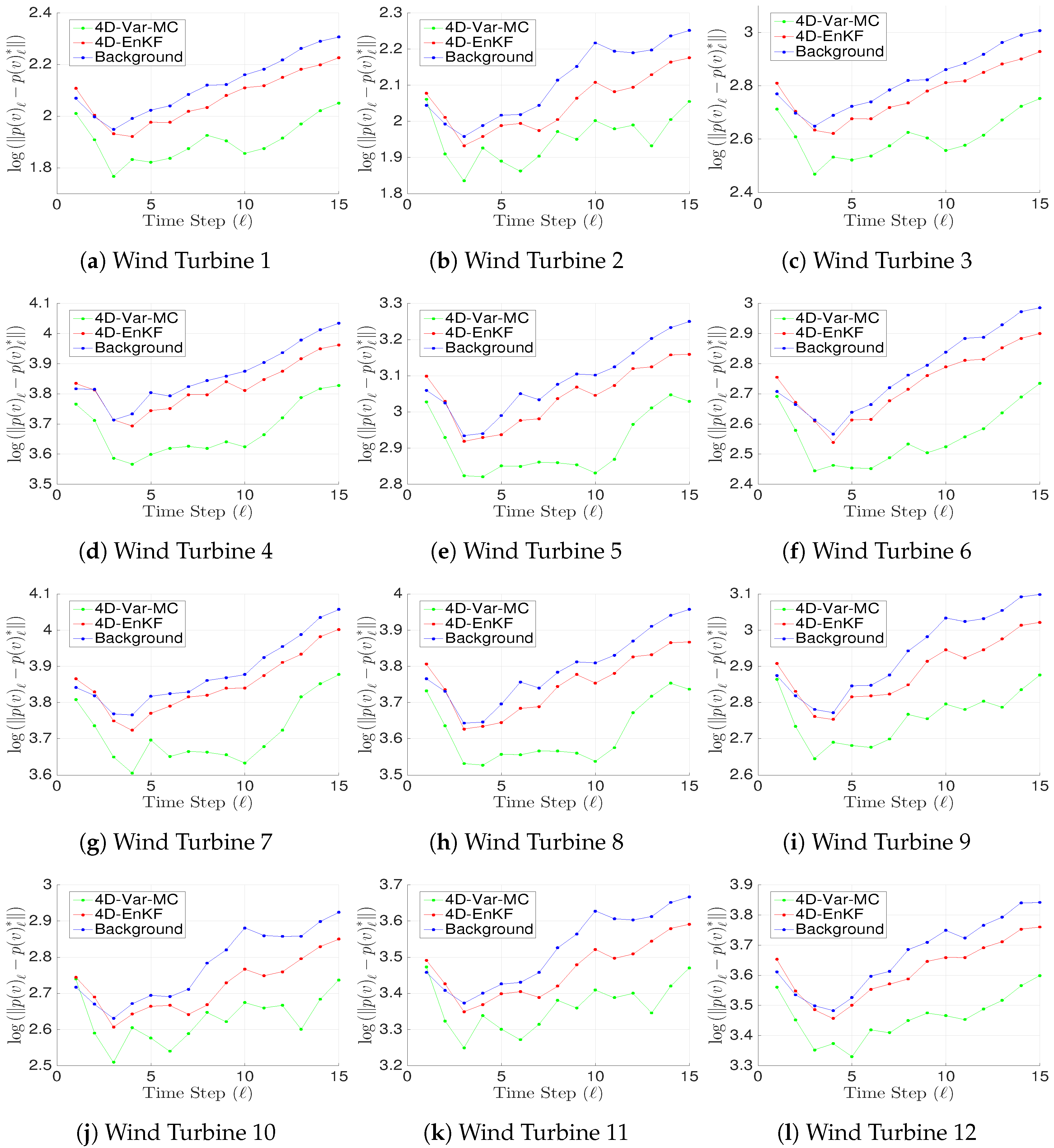
The L 2 error norms (21) of wind-energy-potential estimations for an ensemble size of N = 20 is shown in Figure 3. We employ a log scale in the y axis to render the text easier to read. As can be seen, for all WTGs, the compared filter implementations provide better estimates of potential generations than those obtained by pure forecasts, as should be expected. Thus, regardless of the employed DA method, the accuracy of forecasts can be improved by injecting real observations of the dynamical system. This can be beneficial for taking actions on whether to employ or not green sources of energy during, for instance, industrial operations. In all cases, on average, the estimated analysis trajectories in the 4D-Var-MC context outperform those computed by the 4D-EnKF formulation. In the 4D-Var-MC, the dimension of control spaces equals those of model one; therefore, we have enough degrees of freedom to capture most of the directions where errors grow faster. This allows our proposed implementation to properly correct initial background states with the information brought by observations in time. Besides, the initial analysis state (initial condition of the initial value problem) relies on the quality of the estimated background error correlations:
Δ x 0 a B 0 1 x a x b B ^ 0 1 x a x b V ^ 0 T · Γ ^ 0 1 · V ^ 0 1 2 .
As is proven in [26] [Theorem 1], the precision matrix estimator (8a) converges to the actual precision matrix B 0 1 as long as log ( n ) / N goes to zero. This value, under the current experimental settings, reads ∼0.170, which can explain as well why the accuracy of the 4D-EnKF-MC method is better than that of the 4D-EnKF. On the other hand, the control space in the 4D-EnKF formulation relies on the ensemble size, whose dimension is much lesser than that of the model one. Consequently, this sub-space can be highly sensitive to sampling noise, which can create spurious correlations among distant model components. Besides, there is no guaranty that such sub-space can capture the leading directions where errors grow faster. This results in the poor estimation of the analysis increments of the initial ensemble mean and, as a direct consequence, the analysis members of the initial ensemble. For this reason, the benefits of increasing the number of model realizations are just evident in the 4D-EnKF context; for instance, the accuracy of this formulation improves drastically as the ensemble size increases. The Table 3 provides an overview of the compared filter implementations in terms of performance (RMSE values) and all parameter configurations, RMSE values are computed based on the analysis trajectory (estimated initial condition). It is clear that, on average, our proposed filter implementation outperforms the traditional 4D-EnkF one in terms of accuracy. In general, both filters formulations can improve their performance as the ensemble size is increased.
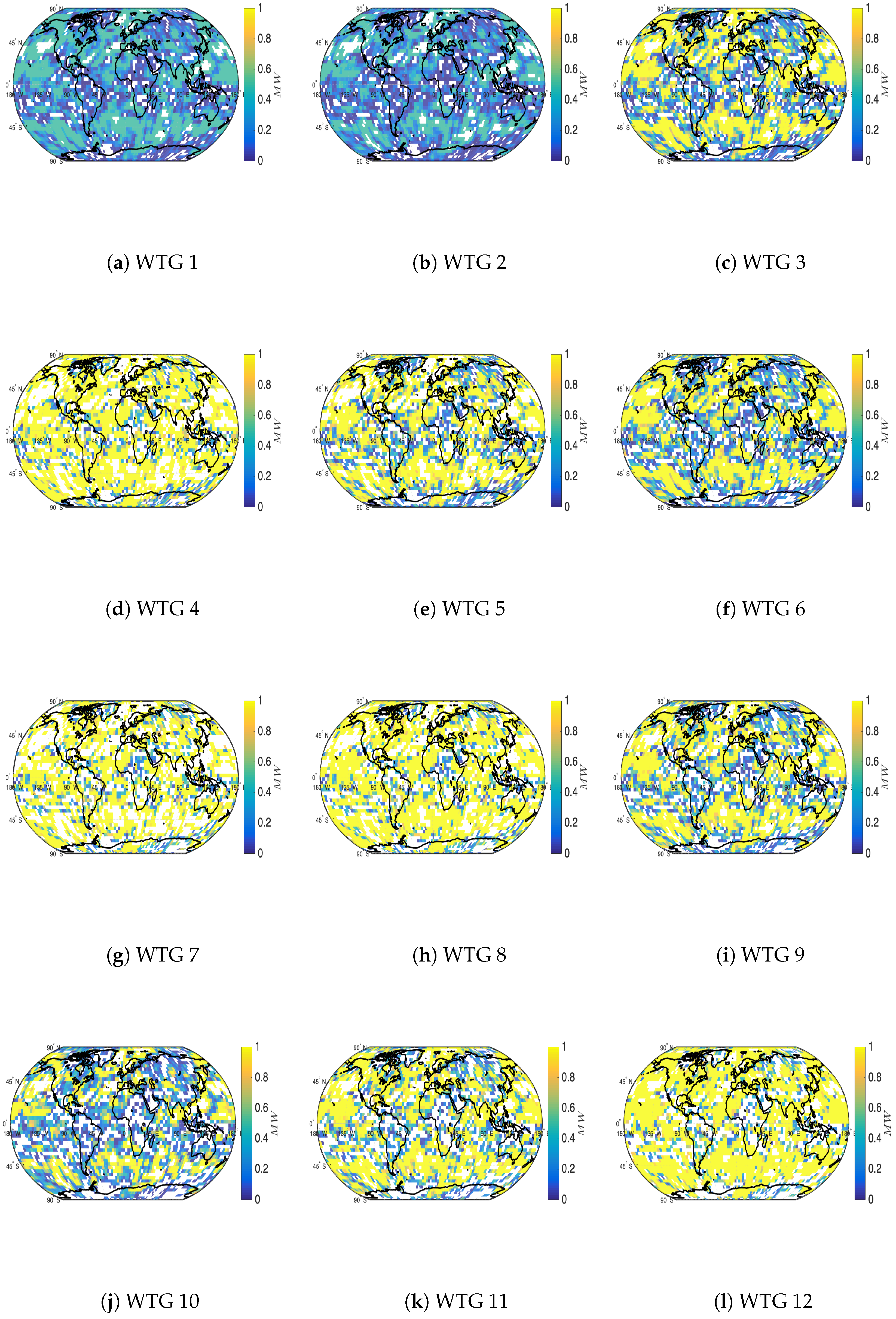
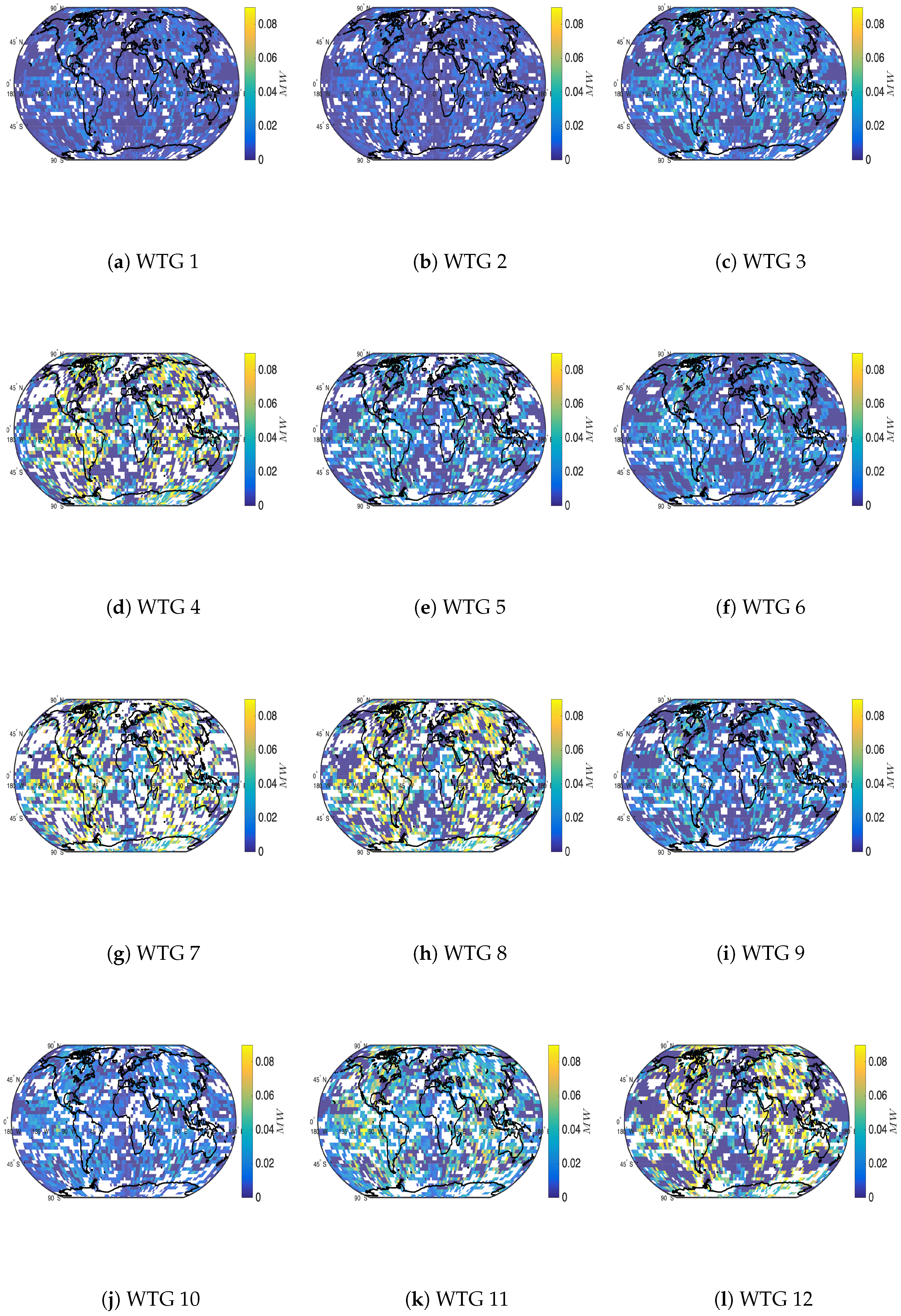
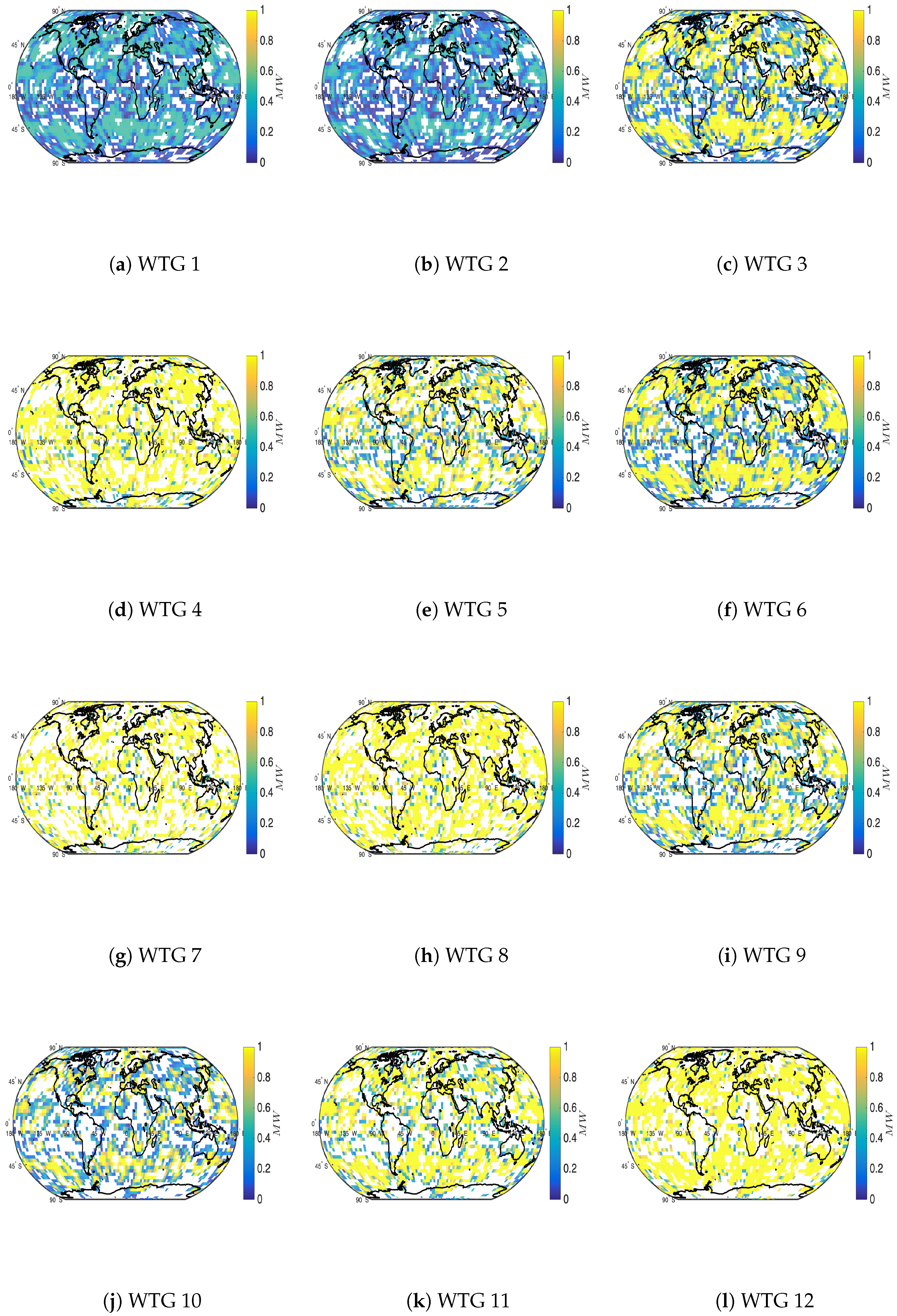
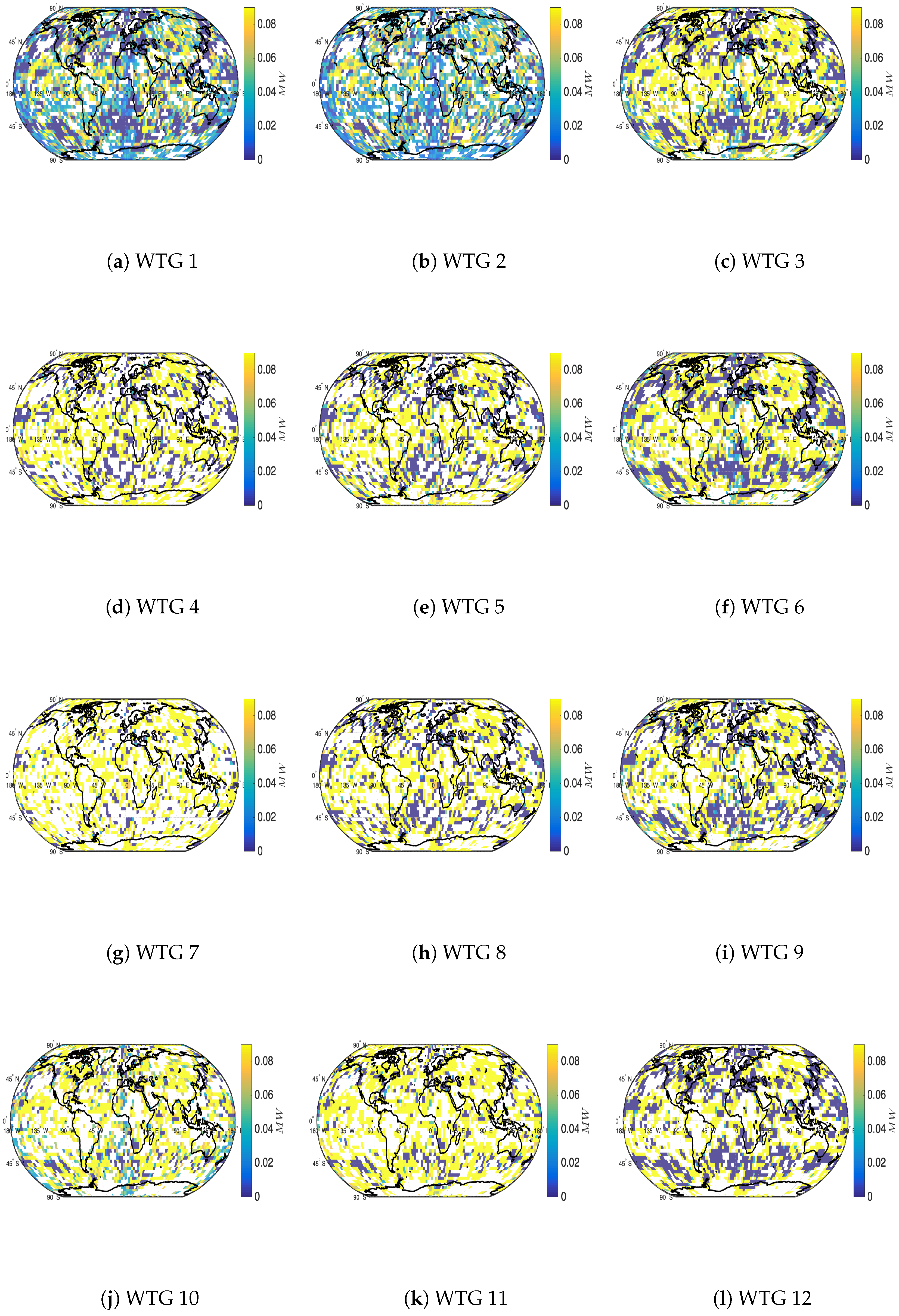
In Figure 4, snapshots of the estimated initial wind-energy-potential are shown for the proposed 4D-Var-MC method. Their corresponding standard deviations of errors (based on analysis ensembles) are shown in Figure 5. Recall that this initial state is our estimate of the initial condition in the optimization problem (3). As can be expected, most of the wind-energy-potential is produced on the ocean where wind speeds get the largest rise for all wind turbines. This serves as a validation test since no wind farms (turbines) can be placed under such a place. However, countries well-known for their potential capacities are just evident in these results, for instance, countries such as those from Latin American and the Caribbean and Africa. Moreover, by taking a close look at standard deviations, one can see that forecasts are obtained with low uncertainties for all filter implementations. This, together with the RMSE results, show that the proposed framework can be employed to estimate wind energy potentials with high accuracy and low variations.
Notice, green sources of energy such as those based on wind speeds are impacted by three observable conditions (which can be implicitly evidenced in our numerical results): variability, unpredictability, and placement. Variability obeys to the fact that as time moves forward, wind speeds can drastically vary, this impacts the potential energy that can be generated by WTGs. Regardless the DA method employed to estimate wind potential capacities, unpredictability is always present: numerical forecasts are imperfect and even more, uncertain. Placement of WTGs is crucial, as can be seen in Figure 4, no all WTGs can properly work in different zones of the globe, this is, electrical power via WTGs can drastically vary from one place to other. We can stood out the importance of employing WTGs as sources of energy based on wind speeds in different regions of the globe but, we cannot argue which turbine is better than others. To do this analysis, we should consider other relevant factors such as wind speed variability, WTGs constraints, and economic considerations, the last two are out of the scope of our analysis.
Consider, again, the WTG parameters reported in the Table 1 and the initial snapshots reported in Figure 4 and Figure 5. Note that, in most places in the globe, WTGs 1 and 2 can be installed to guaranty electrical power from wind speeds; these WTGs are the ones with rate-capacity 0.5. Note that, as the cut-in wind speed and the rate-capacity increase, the electrical energy generation of WTGs can be impacted. For instance, near the poles, the power generation is almost null for WTGs with the largest cut-in wind speed parameters. WTGs with rated-capacity of 1 are the ones that have large variability across different places in the world. Lastly, the largest amount of energy across different places in the domain can be obtained for WTGs with the largest rate-capacity values. However, WTGs with low rate-capacity values are the ones whose numerical forecasts are obtained with lesser variability (i.e., in Figure 5 the standard deviation of errors has a homogeneous behavior across different regions of the domain). As the rate-capacity increases, the variance of the standard deviation of errors increases as well. This means, more variability of errors can be evidenced across different parts of the world. Thus, WTGs with large rate capacities provide forecasts with a large amount of clean energy, but these come with large uncertainties in certain regions of the world, which can difficult decision making.

4.2. Single Observations across Observation Times

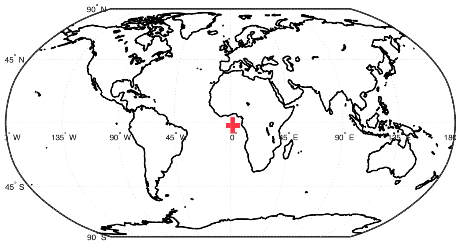
In this section, we briefly discuss the performance of our proposed 4D-EnKF-MC method by using a single observation test. We hold the same experimental settings as those in Section 4.1 and report the estimation errors in the initial conditions via L 2 norms (21). The single observation, across all observation times, is placed as is shown in Figure 6.
In the Table 4, we can clearly seen the advantages of employing the control space (11) instead of the traditional approach based on the ensemble sub-space (5). For instance, for WTG with low rate-capacity, error differences are of one order of magnitude. In Figure 7 and Figure 8, we report the potential energy estimation and the uncertainty of each component (as the standard deviation of errors from the initial members of the analysis ensemble). As can be seen, low-rate capacity WTGs such as the WTG 1 and the WTG2 provide estimates whose error dispersion is small. Again, as the rate-capacity increases, the spread of ensemble members grow. The accuracy of the proposed method obeys to the fact that the precision matrix is full-rank, well-conditioned, and even more localized. Thus, the impact of spurious correlations is mitigated in the analysis increments of the initial ensemble.

5. Conclusions

We propose a 4D-Var ensemble-based data assimilation framework for wind energy potential estimation. In this formulation, in the 4D-Var context, the intrinsic need of adjoint models is avoided via the use of an ensemble of model realizations. These ensembles are employed to build control spaces onto which analysis increments are estimated. Control spaces are built via a modified Cholesky decomposition. The particular structure of this estimator allows for a matrix-free implementation of the proposed filter formulation. Experimental tests are performed, making use of wind turbines catalogs and the Atmospheric General Circulation Model Speedy. The results reveal that our proposed framework can properly estimate wind energy potential capacities within reasonable accuracies in terms of Root-Mean-Square-Error, and even more, these estimations are better than those of traditional 4D-Var ensemble-based methods. Besides, Wind Turbine Generators (WTGs) with low rate-capacity are the ones which provide homogeneous behavior of error estimations around the globe. As the rate-capacity increases, the potential energy increases as well, but the error dispersion of ensemble members grow, which can difficult decision-making processes. Of course, rate-capacity is just a single parameter of many in the WTG context, and we do not consider, for instance, economic aspects in our study, which can be crucial for deciding whether or not to employ green sources of energy.

Author Contributions

E.D.N.-R., and J.C.C.-S. derive the 4D-Var-MC filter and its matrix-free implementation; E.D.N.-R., J.C.C.-S., and L.G.G.-R. conceived and designed the experiments; L.G.G.-R., and J.C.C.-S. performed the experiments; E.D.N.-R., A.H. and J.C.C.-S. analyzed the data; E.D.N.-R., and J.C.C.-S. wrote the paper. All authors have read and agreed to the published version of the manuscript.

Funding

This research received no external funding.

Acknowledgments

This work was supported by the Applied Math and Computer Science Laboratory at Universidad del Norte (AML-CS).

Conflicts of Interest

The authors declare no conflict of interest.

References

  1. Nino-Ruiz, E.D. Implicit surrogate models for trust region based methods. J. Comput. Sci. 2018, 26, 164–274. [Google Scholar] [CrossRef]
  2. Nino-Ruiz, E.D.; Cheng, H.; Beltran, R. A Robust Non-Gaussian Data Assimilation Method for Highly Non-Linear Models. Atmosphere 2018, 9, 126. [Google Scholar] [CrossRef] [Green Version]
  3. Lorenc, A.C. The potential of the ensemble Kalman filter for NWP—A comparison with 4D-Var. Q. J. R. Meteorol. Soc. A J. Atmos. Sci. Appl. Meteorol. Phys. Oceanogr. 2003, 129, 3183–3203. [Google Scholar] [CrossRef]
  4. Lorenc, A.C. Modelling of error covariances by 4D-Var data assimilation. Q. J. R. Meteorol. Soc. A J. Atmos. Sci. Appl. Meteorol. Phys. Oceanogr. 2003, 129, 3167–3182. [Google Scholar] [CrossRef]
  5. Fay, M.; Andres, L.A.; Fox, C.; Narloch, U.; Slawson, M. Rethinking Infrastructure in Latin America and the Caribbean: Spending Better to Achieve More; World Bank Publications: Washington, DC, USA, 2017. [Google Scholar]
  6. Del Río, P.; Burguillo, M. Assessing the impact of renewable energy deployment on local sustainability: Towards a theoretical framework. Renew. Sustain. Energy Rev. 2008, 12, 1325–1344. [Google Scholar] [CrossRef]
  7. Vergara, W.; Isbell, P.; Rios, A.R.; Gómez, J.R.; Alves, L. Societal Benefits from Renewable Energy in Latin America and the Caribbean; Technical report; Inter-American Development Bank: Washington, DC, USA, 2014. [Google Scholar]
  8. Munoz, F.D.; Wogrin, S.; Oren, S.S.; Hobbs, B.F. Economic Inefficiencies of Cost-based Electricity Market Designs. In Proceedings of the Heading Towards Sustainable Energy Systems: Evolution or Revolution? 15th IAEE European Conference International Association for Energy Economics, Vienna, Austria, 3–6 September 2017. [Google Scholar]
  9. Griffith-Jones, S.; Spratt, S.; Andrade, R.; Griffith-Jones, E. Investment in Renewable Energy, Fossil Fuel Prices and Policy Implications for Latin America and the Caribbean. 2017. Available online: https://repositorio.cepal.org/handle/11362/41679 (accessed on 3 January 2020).
  10. Gustafsson, N.; Bojarova, J. Four-dimensional ensemble variational (4D-En-Var) data assimilation for the high resolution limited area model (HIRLAM). Nonlinear Process. Geophys. 2014, 21, 745–762. [Google Scholar] [CrossRef] [Green Version]
  11. Stengel, M.; Undén, P.; Lindskog, M.; Dahlgren, P.; Gustafsson, N.; Bennartz, R. Assimilation of SEVIRI infrared radiances with HIRLAM 4D-Var. Q. J. R. Meteorol. Soc. A J. Atmos. Sci. Appl. Meteorol. Phys. Oceanogr. 2009, 135, 2100–2109. [Google Scholar] [CrossRef]
  12. Gustafsson, N. Discussion on ‘4D-Var or EnKF?’. Tellus A Dyn. Meteorol. Oceanogr. 2007, 59, 774–777. [Google Scholar] [CrossRef] [Green Version]
  13. Nino-Ruiz, E.D.; Sandu, A. Ensemble Kalman filter implementations based on shrinkage covariance matrix estimation. Ocean Dyn. 2015, 65, 1423–1439. [Google Scholar] [CrossRef] [Green Version]
  14. Houtekamer, P.L.; Mitchell, H.L. Data assimilation using an ensemble Kalman filter technique. Mon. Weather Rev. 1998, 126, 796–811. [Google Scholar] [CrossRef]
  15. Stroud, J.R.; Katzfuss, M.; Wikle, C.K. A Bayesian adaptive ensemble Kalman filter for sequential state and parameter estimation. Mon. Weather Rev. 2018, 146, 373–386. [Google Scholar] [CrossRef]
  16. Goodliff, M.; Amezcua, J.; Van Leeuwen, P.J. Comparing hybrid data assimilation methods on the Lorenz 1963 model with increasing non-linearity. Tellus A Dyn. Meteorol. Oceanogr. 2015, 67, 26928. [Google Scholar] [CrossRef]
  17. Nino-Ruiz, E.D.; Sandu, A. A derivative-free trust region framework for variational data assimilation. J. Comput. Appl. Math. 2016, 293, 164–179. [Google Scholar] [CrossRef]
  18. Greybush, S.J.; Kalnay, E.; Miyoshi, T.; Ide, K.; Hunt, B.R. Balance and ensemble Kalman filter localization techniques. Mon. Weather Rev. 2011, 139, 511–522. [Google Scholar] [CrossRef]
  19. Chen, Y.; Oliver, D.S. Cross-covariances and localization for EnKF in multiphase flow data assimilation. Comput. Geosci. 2010, 14, 579–601. [Google Scholar] [CrossRef]
  20. Lei, L.; Whitaker, J.S.; Bishop, C. Improving assimilation of radiance observations by implementing model space localization in an ensemble Kalman filter. J. Adv. Model. Earth Syst. 2018, 10, 3221–3232. [Google Scholar] [CrossRef] [Green Version]
  21. Anderson, J.L. An ensemble adjustment Kalman filter for data assimilation. Mon. Weather Rev. 2001, 129, 2884–2903. [Google Scholar] [CrossRef] [Green Version]
  22. Han, Y.; Zhang, J.; Sun, D. Error control and adjustment method for underwater wireless sensor network localization. Appl. Acoust. 2018, 130, 293–299. [Google Scholar] [CrossRef]
  23. Anderson, J.L. A Nonlinear Rank Regression Method for Ensemble Kalman Filter Data Assimilation. Mon. Weather Rev. 2019, 147, 2847–2860. [Google Scholar] [CrossRef]
  24. Levina, E.; Rothman, A.; Zhu, J. Sparse estimation of large covariance matrices via a nested lasso penalty. Ann. Appl. Stat. 2008, 2, 245–263. [Google Scholar] [CrossRef]
  25. Nino-Ruiz, E.D.; Sandu, A.; Deng, X. A parallel implementation of the ensemble Kalman filter based on modified Cholesky decomposition. J. Comput. Sci. 2017. [Google Scholar] [CrossRef] [Green Version]
  26. Nino-Ruiz, E.D.; Sandu, A.; Deng, X. An Ensemble Kalman Filter Implementation Based on Modified Cholesky Decomposition for Inverse Covariance Matrix Estimation. SIAM J. Sci. Comput. 2018, 40, A867–A886. [Google Scholar] [CrossRef]
  27. Bickel, P.J.; Levina, E. Regularized estimation of large covariance matrices. Ann. Stat. 2008, 36, 199–227. [Google Scholar] [CrossRef]
  28. Kopiske, J.; Spieker, S.; Tsatsaronis, G. Value of power plant flexibility in power systems with high shares of variable renewables: A scenario outlook for Germany 2035. Energy 2017, 137, 823–833. [Google Scholar] [CrossRef]
  29. Liu, Z. China’s strategy for the development of renewable energies. Energy Sources Part B Econ. Plan. Policy 2017, 12, 971–975. [Google Scholar] [CrossRef] [Green Version]
  30. Verzijlbergh, R.; De Vries, L.; Dijkema, G.; Herder, P. Institutional challenges caused by the integration of renewable energy sources in the European electricity sector. Renew. Sustain. Energy Rev. 2017, 75, 660–667. [Google Scholar] [CrossRef] [Green Version]
  31. Xie, K.; Billinton, R. Determination of the optimum capacity and type of wind turbine generators in a power system considering reliability and cost. IEEE Trans. Energy Convers. 2010, 26, 227–234. [Google Scholar] [CrossRef]
  32. Wiser, R. Annual Report on US Wind Power Installation, Cost, and Performance Trends: 2007; Technical report; EERE Publication and Product Library: Washington, DC, USA, 2008. [Google Scholar]
  33. Masters, G.M. Renewable and Efficient Electric Power Systems; John Wiley & Sons: New York, NY, USA, 2013. [Google Scholar]
  34. Amezcua, J.; Kalnay, E.; Williams, P.D. The effects of the RAW filter on the climatology and forecast skill of the SPEEDY model. Mon. Weather Rev. 2011, 139, 608–619. [Google Scholar] [CrossRef] [Green Version]
  35. Michalakes, J.; Dudhia, J.; Gill, D.; Henderson, T.; Klemp, J.; Skamarock, W.; Wang, W. The weather research and forecast model: Software architecture and performance. In Use of High Performance Computing in Meteorology; World Scientific: Singapore, 2005; pp. 156–168. [Google Scholar]
  36. Michalakes, J.; Chen, S.; Dudhia, J.; Hart, L.; Klemp, J.; Middlecoff, J.; Skamarock, W. Development of a next-generation regional weather research and forecast model. In Developments in Teracomputing; World Scientific: Singapore, 2001; pp. 269–276. [Google Scholar]
  37. Nino-Ruiz, E.D.; Sandu, A.; Anderson, J. An efficient implementation of the ensemble Kalman filter based on an iterative Sherman–Morrison formula. Stat. Comput. 2015, 25, 561–577. [Google Scholar] [CrossRef] [Green Version]
  38. Nino-Ruiz, E. A matrix-free posterior ensemble kalman filter implementation based on a modified cholesky decomposition. Atmosphere 2017, 8, 125. [Google Scholar] [CrossRef] [Green Version]
  39. Bracco, A.; Kucharski, F.; Kallummal, R.; Molteni, F. Internal variability, external forcing and climate trends in multi-decadal AGCM ensembles. Clim. Dyn. 2004, 23, 659–678. [Google Scholar] [CrossRef]
  40. Miyoshi, T. The Gaussian approach to adaptive covariance inflation and its implementation with the local ensemble transform Kalman filter. Mon. Weather Rev. 2011, 139, 1519–1535. [Google Scholar] [CrossRef]
  41. Molteni, F. Atmospheric simulations using a GCM with simplified physical parametrizations. I: Model climatology and variability in multi-decadal experiments. Clim. Dyn. 2003, 20, 175–191. [Google Scholar] [CrossRef]
  42. Kucharski, F.; Molteni, F.; Bracco, A. Decadal interactions between the western tropical Pacific and the North Atlantic Oscillation. Clim. Dyn. 2006, 26, 79–91. [Google Scholar] [CrossRef]
  43. Miyoshi, T.; Kondo, K.; Imamura, T. The 10,240-member ensemble Kalman filtering with an intermediate AGCM. Geophys. Res. Lett. 2014, 41, 5264–5271. [Google Scholar] [CrossRef]
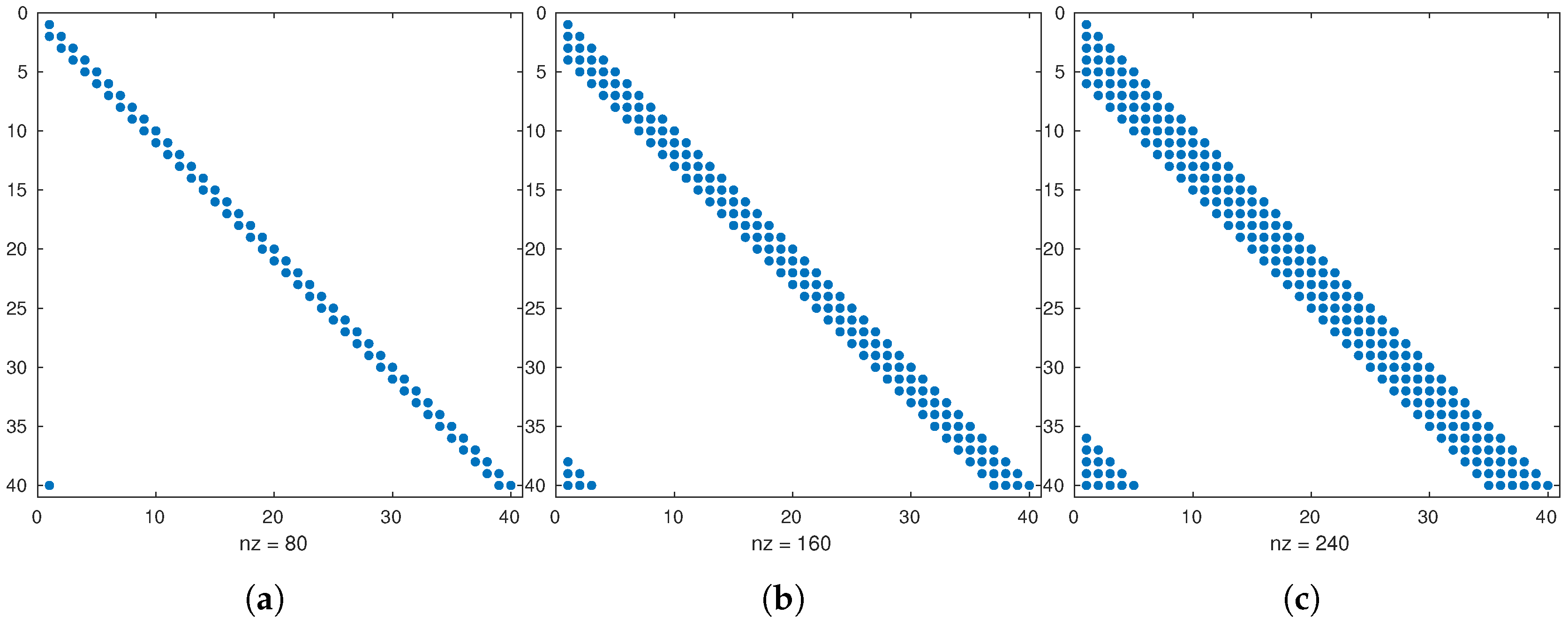
Figure 1. Structure of the Cholesky factor V ^ k as a function of the localization radius δ . (a) δ = 1 ; (b) δ = 3 ; (c) δ = 5 .
Atmosphere 11 00167 g001
Figure 2. Linear observation operator during assimilation steps. Shaded regions denote observed components (observations) from the model state. The operator is replicated across all numerical layers.
Atmosphere 11 00167 g002
Figure 3. Error norms of wind energy potential estimations for the compared filter implementations. The ensemble size reads N = 20 . 12 wind turbines are employed for the experiments. Units are in MW. (a) Wind Turbine 1; (b) Wind Turbine 2; (c) Wind Turbine 3; (d) Wind Turbine 4; (e) Wind Turbine 5; (f) Wind Turbine 6; (g) Wind Turbine 7; (h) Wind Turbine 8; (i) Wind Turbine 9; (j) Wind Turbine 10; (k) Wind Turbine 11; (l) Wind Turbine 12.
Atmosphere 11 00167 g003
Figure 4. Mean of wind energy potentials for the 4D-Var-MC implementations. The number of ensemble members N = 20 . White regions denote no wind-energy-potential generation. (a) WTG 1; (b) WTG 2; (c) WTG 3; (d) WTG 4; (e) WTG 5; (f) WTG 6; (g) WTG 7; (h) WTG 8; (i) WTG 9; (j) WTG 10; (k) WTG 11; (l) WTG 12.
Atmosphere 11 00167 g004
Figure 5. Mean of wind energy potentials for the 4D-Var-MC implementations. The number of ensemble members N = 20 . White regions denote no wind-energy-potential generation. (a) WTG 1; (b) WTG 2; (c) WTG 3; (d) WTG 4; (e) WTG 5; (f) WTG 6; (g) WTG 7; (h) WTG 8; (i) WTG 9; (j) WTG 10; (k) WTG 11; (l) WTG 12.
Atmosphere 11 00167 g005
Figure 6. Observation operator across assimilation steps. A single observation (red cross) is placed during the experiments.
Atmosphere 11 00167 g006
Figure 7. Mean of wind energy potentials for the 4D-Var-MC implementations. The number of ensemble members N = 20 . White regions denote no wind-energy-potential generation. The number of observations reads 1. (a) WTG 1; (b) WTG 2; (c) WTG 3; (d) WTG 4; (e) WTG 5; (f) WTG 6; (g) WTG 7; (h) WTG 8; (i) WTG 9; (j) WTG 10; (k) WTG 11; (l) WTG 12.
Atmosphere 11 00167 g007
Figure 8. Mean of wind energy potentials for the 4D-Var-MC implementations. The number of ensemble members N = 20 . White regions denote no wind-energy-potential generation. The number of observations reads 1. (a) WTG 1; (b) WTG 2; (c) WTG 3; (d) WTG 4; (e) WTG 5; (f) WTG 6; (g) WTG 7; (h) WTG 8; (i) WTG 9; (j) WTG 10; (k) WTG 11; (l) WTG 12.
Atmosphere 11 00167 g008
Table 1. WTG Unit Parameters.
TypeRated Capacity (MW) v c (km/h) v r (km/h) v f (km/h)Capital Cost M & O
WTG 10.5104080135036
WTG 20.5104570135036
WTG 31124080125035
WTG 42123055112030
WTG 51133360122033
WTG 61144090125032
WTG 72153350110035
WTG 82153360110030.5
WTG 91153770120032
WTG 101184870125032
WTG 112184570110030
WTG 122183575110030
Table 2. Physical variables of the AT-GCM Speedy model.
NameNotationUnitsNumber of Layers
TemperatureTK7
Zonal Wind Componentum/s7
Meridional Wind Componentvm/s7
Specific HumidityQg/kg7
PressureTK1
Table 3. Root-Mean-Square-Error values of wind energy potential estimations. Two ensemble sizes are tried during the experiments.
N
2040
Wind Turbine Generator (WTG)4D-EnKF4D-Var-MC4D-EnKF4D-Var-MC
WTG 10.117130.099270.112110.10098
WTG 20.114810.103910.111430.10596
WTG 30.236080.200080.225970.20354
WTG 40.675970.585240.650880.59049
WTG 50.310100.270930.296920.27475
WTG 60.228080.190580.218760.19488
WTG 70.694120.606090.671700.61034
WTG 80.629010.549010.602320.55692
WTG 90.265030.233050.255540.23756
WTG 100.224250.204660.217970.20872
WTG 110.472210.426310.458240.43497
WTG 120.550060.470310.529810.47967
Table 4. L 2 error norms of wind energy potential estimations at the initial analysis member. Two ensemble sizes are tried during the experiments.
Data Assimilation Method
Wind Turbine Generator (WTG)4D EnKf4D EnKf-Cho
WTG 110.44528.5893
WTG 210.31498.4186
WTG 321.057017.3117
WTG 458.118649.0419
WTG 527.298622.9304
WTG 620.438816.4551
WTG 759.429650.3057
WTG 855.322046.4524
WTG 923.526519.2920
WTG 1020.234216.5172
WTG 1142.430834.6328
WTG 1248.375640.4795