Article

Spring Season in Western Nepal Himalaya is not yet Warming: A 400-Year Temperature Reconstruction Based on Tree-Ring Widths of Himalayan Hemlock (Tsuga dumosa)

1
Friedrich-Alexander-Universität Erlangen-Nürnberg, Institut für Geographie, Wetterkreuz 15, 91058 Erlangen, Germany
2
Key Laboratory of Tropical Forest Ecology, Xishuangbanna Tropical Botanical Garden, Chinese Academy of Sciences, Mengla 666303, China
3
Warnell School of Forestry and Natural Resources, University of Georgia, 180 East Green Street Athens, Athens, GA 30602, USA
4
Nepal Academy of Science and Technology, Khumaltar, Lalitpur 44700, Nepal
5
Forest Research and Training Centre, Babarmahal, Kathmandu 44600, Nepal
6
Key Laboratory of Alpine Ecology, Institute of Tibetan Plateau Research, Chinese Academy of Sciences, Beijing 100101, China
*
Author to whom correspondence should be addressed.
Atmosphere 2020, 11(2), 132; https://doi.org/10.3390/atmos11020132
Submission received: 9 January 2020 / Accepted: 21 January 2020 / Published: 24 January 2020
(This article belongs to the Special Issue Climates of the Himalayas: Present, Past and Future)

Abstract

:
The Himalayan region has already witnessed profound climate changes detectable in the cryosphere and the hydrological cycle, already resulting in drastic socio-economic impacts. We developed a 619-yea-long tree-ring-width chronology from the central Nepal Himalaya, spanning the period 1399–2017 CE. However, due to low replication of the early part of the chronology, only the section after 1600 CE was used for climate reconstruction. Proxy climate relationships indicate that temperature conditions during spring (March–May) are the main forcing factor for tree growth of Tsuga dumosa at the study site. We developed a robust climate reconstruction model and reconstructed spring temperatures for the period 1600–2017 CE. Our reconstruction showed cooler conditions during 1658–1681 CE, 1705–1722 CE, 1753–1773 CE, 1796–1874 CE, 1900–1936 CE, and 1973 CE. Periods with comparably warmer conditions occurred in 1600–1625 CE, 1633–1657 CE, 1682–1704 CE, 1740–1752 CE, 1779–1795 CE, 1936–1945 CE, 1956–1972 CE, and at the beginning of the 21st century. Tropical volcanic eruptions showed only a sporadic impact on the reconstructed temperature. Also, no consistent temperature trend was evident since 1600 CE. Our temperature reconstruction showed positive teleconnections with March–May averaged gridded temperature data for far west Nepal and adjacent areas in Northwest India and on the Southwest Tibetan plateau. We found spectral periodicities of 2.75–4 and 40–65 years frequencies in our temperature reconstruction, indicating that past climate variability in central Nepal might have been influenced by large-scale climate modes, like the Atlantic Multi-decadal Oscillation, the North Atlantic Oscillation, and the El Niño-Southern Oscillation.

1. Introduction

The impact of climate change in the central Himalayan region of Nepal is more pronounced compared to other regions at similar latitudes [1] and hence Nepal is experiencing higher rates of temperature increase than the global average [1,2,3,4]. However, the observed warming rates show significant spatial variability, with a more pronounced warming trend in higher altitudes [1,5]. According to the Fourth Assessment Report (AR) of the Intergovernmental Panel on Climate Change (IPCC), climate change has significant effects on natural systems as well as on human societies worldwide [6]. Almost every climate model indicates a further pronounced warming trend in the future, associated to a corresponding change in the hydro-climate and in the frequency, severity, and nature of extreme events, such as drought and heavy precipitation [7,8]. Biodiversity, as an important component of the environment, is not unaffected by these impacts. Extreme climatic events are now accepted to play a major role in current and future ecosystem dynamics [9,10]. Additionally, the impact of climate change can already be monitored in changes in species distribution, population structures, ecological zone shifts, species composition of ecosystems, phenology, and growing season on a regional as well as on a global scale [2,3,11,12,13,14,15].
Nepal is a mountainous country with a limited number of available meteorological stations. Available stations are mostly situated at lower elevations and have only a short temporal coverage of a few decades (longest instrumental data available from the 1950s from the Kathmandu airport) [16]. These deficiencies in the available instrumental datasets lead to an insufficient ability to quantify long-term trends and recent impacts of climate change on the local level, which are of great importance for policy and decision makers [1,17]. To fill these data gaps, there are prospects of using different proxy data, among which tree rings have been proven to be one of the most promising [18]. This holds especially true for Nepal, which hosts many tree species with proven dendrochronological potential [19,20,21] in high-elevation ecosystems, which are the crucial region for detecting climate change patterns on regional scales [22]. However, to date, only four temperature reconstructions [19,23,24], one precipitation and four moisture index [25,26,27,28,29] reconstructions, have been conducted for the central Nepalese Himalaya. Although available temperature reconstructions used different tree species from different locations, they share common low-frequency variations. However, in terms of high-frequency variations, they are quite heterogeneous. For instance, Cook et al. [19] and Sano et al. [23] reported a decrease in summer temperatures in the recent decades, whereas Thapa et al. [24] found a warming trend. The extreme and complex topography of Nepal leads to substantial spatial variations in climatic variables, such as radiation, air temperature, and precipitation [30], resulting in a high variability of local climatic conditions. Therefore, single climate reconstructions are not capable of capturing the geographical heterogeneity of the country, making further dendroclimatic studies essential to gain deeper insight into the spatio-temporal picture of climate change in Nepal.
The Himalayan Hemlock (Tsuga dumosa, Eichl.) is a native Himalayan conifer tree species disseminated in a wide area from northern India to Southwestern Sichuan (China) and northern Myanmar [31]. It generally grows in the humid cloud forest belt at an elevation range of 2400 to 3000 m a.s.l. [31]. Hemlocks are a slow-growing, long-living, and shade-tolerant species being sensitive to persistent drought [32]. T. dumosa has well-marked growth rings formed by a sharp change in small-celled darker latewood and large-celled light early-wood [31]. The first tree-ring chronology of T. dumosa was established by Bhattacharyya et al. [21]. Cook et al. [19] included this species in a multi-species composite chronology for the whole of Nepal used for February–June temperature reconstruction. In the same study, Cook et al. [19] presented the longest Hemlock chronology from eastern Nepal, spanning from 856–1996 CE (1141 years). Recently, Bhandari et al. [28] reconstructed a 307-year-long standardized precipitation-evapotranspiration index (SPEI) series from far-western Nepal based on a tree-ring chronology of T. dumosa. In Yunnan (China), T. dumosa chronologies were used for the reconstruction of PDSI-based (Palmer drought severity index) drought variability for March–May [33] and May–June [34], and the relative humidity of the spring season (February–April) [35]. Recently, Borgaonkar et al. [36] reconstructed the summer (July–September) temperature from Sikkim, India. In summary, the climate–growth correlations of T. dumosa indicate that this species is very suitable for studying multiple climatic parameters while the dominant growth-controlling climatic factor depends on the local climatic conditions.
Despite its high dendroclimatic potential, to date, a temperature reconstruction for the central Nepal Himalaya based on ring-width variations of T. dumosa is missing. The present study, therefore, aimed (i) to assess proxy climate relationships of the species in the central Nepalese Himalaya, (ii) to reconstruct past temperature variations in the central Nepalese Himalaya to further contribute to a better understanding of past climate variability in this climatically sensitive region, and (iii) to contribute to a tree-ring chronology network of T. dumosa covering the Himalaya and adjacent mountain regions.

2. Methods

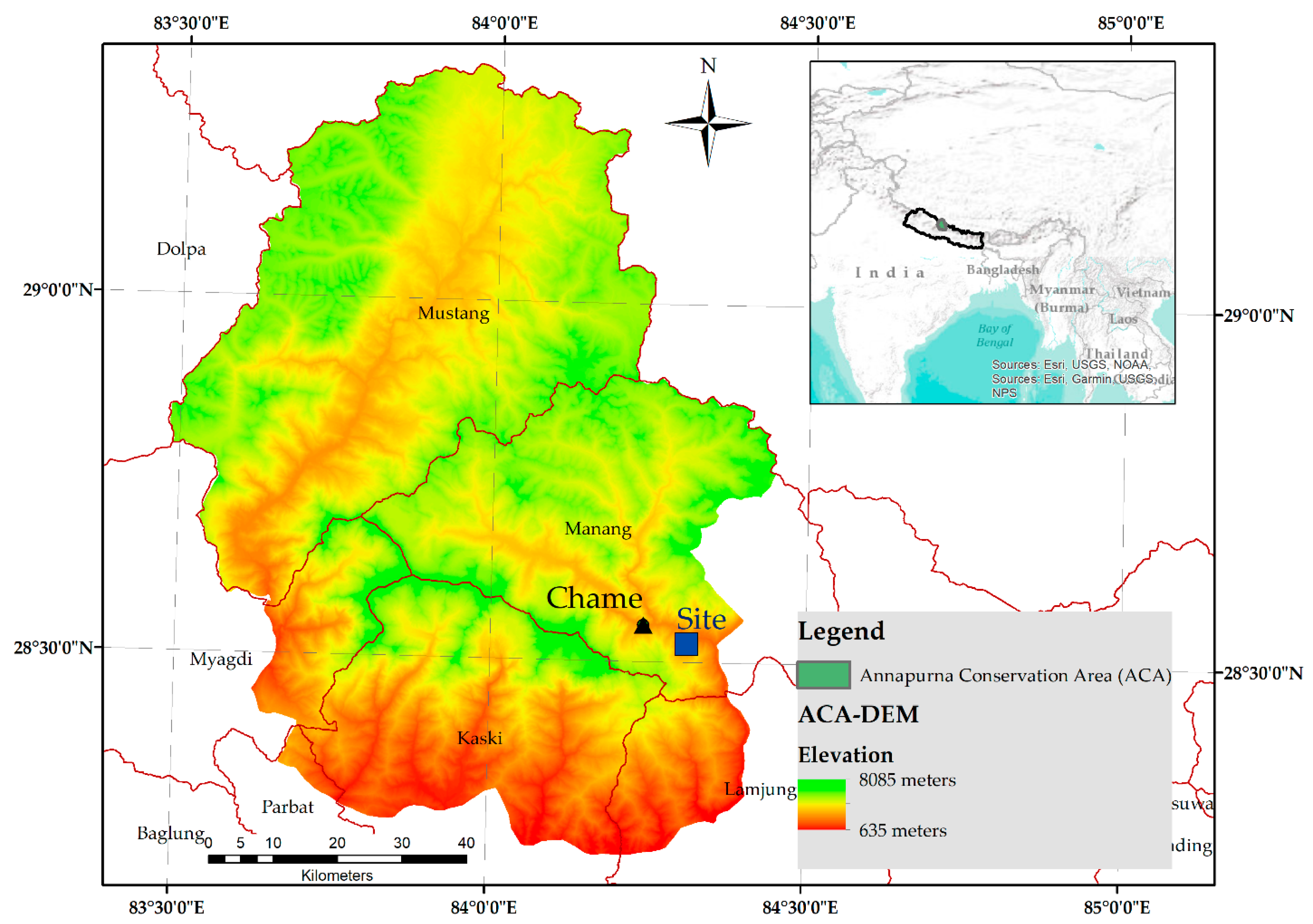
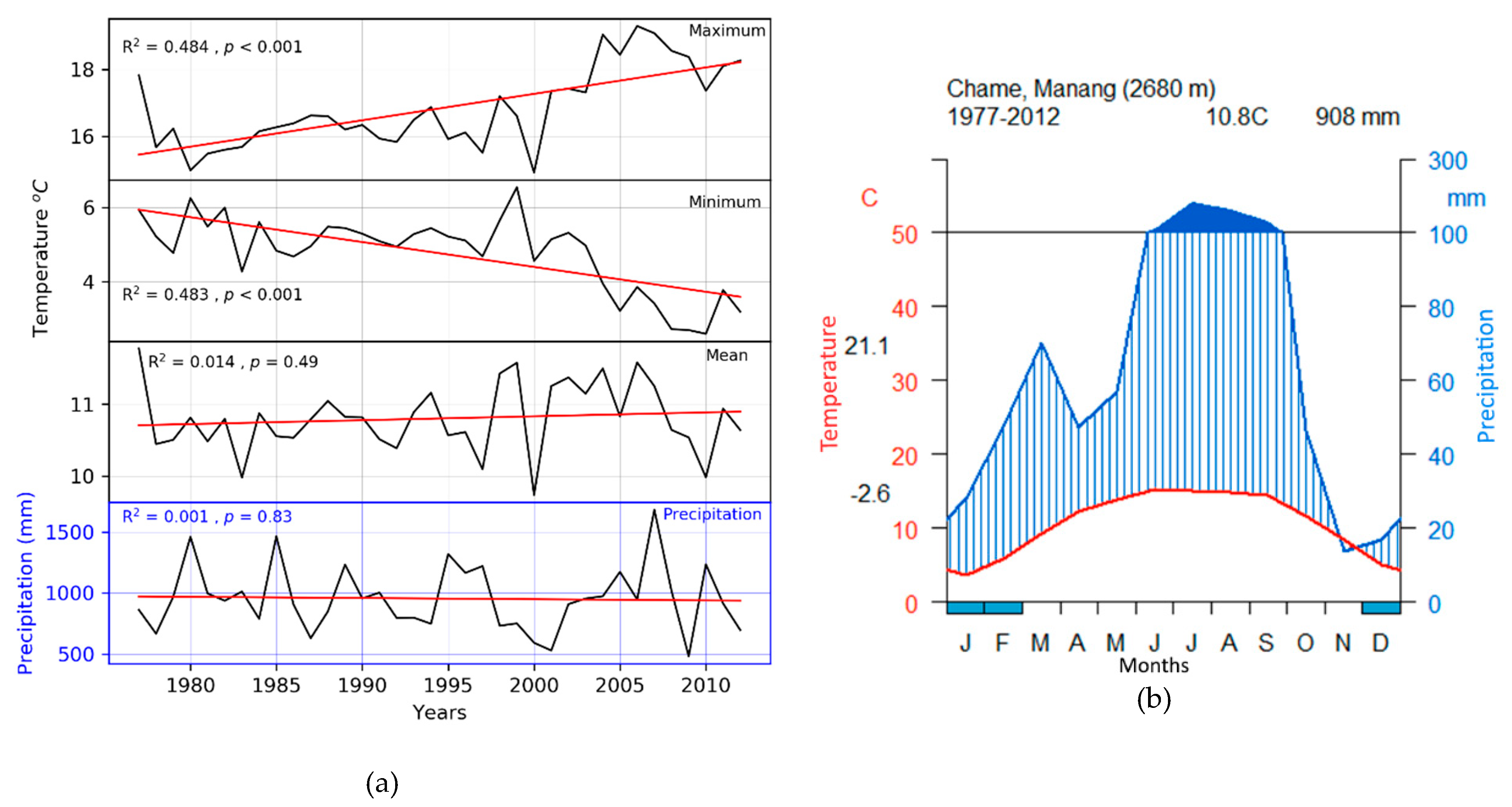
2.1. Study Site and Climate Conditions

The study site is located at the elevation of 2700 m a.s.l. in Timang village (28.52° N, 84.30° E) in the Annapurna Conservation Area (ACA), Manang district, western Nepal (Figure 1). The ACA is the largest protected area of Nepal, with an area of 7629 km2 [37]. This part of ACA is a habitat for different conifer species, including Picea smithiana Boiss., Pinus wallichiana A.B. Jacks, Abies spectabilis (D. Don) Spach, and Taxus sp. mixed with T. dumosa [38]. The sample site is an upper temperate mixed broad-leaved forest at the marginal area between the Trans-Himalayan and High Himalayan regions. The study site is situated in the center of the ACA, about 7 km north of the municipality of Chame.
The northern part of the Manang Himalaya/Manang valley is characterized by a temperate climate with dry winters and warm summers [30]. The analysis of 35-year-long climatic data from the nearest climatic station in Chame shows an average annual temperature and annual total precipitation of 10.8 °C and 908 mm, respectively (Figure 2a). The study area has a pronounced warm and dry spring (March–May) season, followed by a warm and humid summer monsoon season from June to September (Figure 2b). Maximum temperatures in summer can reach 21.1 °C in June, whereas minimum temperatures of −2.6 °C occur in January (Figure 2b). During recent years, there is a marked increase in the average annual maximum temperatures, whereas contemporaneously average annual minimum temperatures showed a decreasing trend (Figure 2a). An analysis of the GIMMS-NDVI dataset for the period 1982 to 2006 indicated an advancement of the vegetation period by 0.31 days per year in the Western Himalayan conifer forest [17].

2.2. Sample Preparation, Ring-Width Measurement, and Development of Chronology

Tree-ring samples were collected during two field visits in April and October 2017 from a mixed conifer forest at a north-east exposed slope. The site consisted of old and evenly aged T. dumosa trees. We aimed to collect two cores from each tree where possible using an increment borer (Haglof, Sweden) at breast height (1.3 m). We avoided the disturbed and unhealthy trees and selected only healthy trees reaching up to the canopy. Due to steep slope angles, taking two cores from each tree was not always possible. In total, 51 tree core samples from 40 trees were collected (Table 1).
Tree-ring width (TRW) was measured under a stereo-microscope and dated with the known date of formation of the outermost ring according to the sampling date. Tree-ring measurement was done using a LINTAB measurement system at a resolution of 0.01 mm with TSAP software (RINNTECH Inc.) [39]. After the measurement of all samples, we used the alignment plot technique to crossdate the individual series by visual matching of tree-ring patterns and the statistical parameters Gleichläufigkeit (GLK., sign test) and t-value [39]. The crossdating quality was checked using the computer program COFECHA [40,41] and, if necessary, tree-ring series were corrected by inserting missing rings in some series. In total, the number of missing rings in our chronology account for 0.158% of all measured rings. Broken samples or samples having individual growth properties caused by local disturbances were discarded from further analysis. For standardization, the individual raw series were first power transformed for variance stabilization [42]. Then, to minimize the removal of any long-term climatic variance, detrending was carried out by applying a signal-free negative exponential curve fitting approach [42] choosing the residual function in RCSigFree 45_v2b (www.ldeo.columbia.edu). The chronology statistics, such as the expressed population signal (EPS), mean correlation between trees (Rbar), and signal to noise ratio (SNR), were considered as a basis for judging the suitability for the further utility of our chronology. Hence, statistics were calculated using a ‘dplR’ [43] package based on R Software [44]. Afterward, the master chronology was calculated using a bi-weight robust mean from all detrended series. The oldest part of our chronology (1399–1599 CE) had to be truncated at the commonly used threshold limit of EPS > 0.85 [45]. Hence, we considered the chronology from 1600–2017 CE, which is reliably replicated for studying climate–growth relationships.

2.3. Climate–Growth Analysis and Climate Reconstruction

The precipitation and temperature data of Chame meteorological station were used for the calibration of the derived growth–climate models. In order to establish a relationship between tree growth and climate variables, we calculated correlation functions and seasonal correlations using the “treeclim” [46] package based on R software.
Based on the results of the growth–climate relationship analysis, we developed a climate reconstruction model using a linear regression model (transfer function) for the reconstruction [47]. As the available instrumental climate data from the nearest station are relatively short, we used the leave-one-out [48] cross-validation test in R software [44] to verify the calibration results. The reconstructed and observed climate data were subject to various statistical tests, i.e., reduction of error (RE) and F-value statistics. A positive value of RE indicates the validity and stability of the reconstruction model. We further calculated the chronology and calibration error [49]. For the chronology error, all the standardized indices of the individual year were sampled with replacement 1000 times, and two-tailed 95% confidence limits of the 1000 bootstrapped mean was estimated. The residual standard error of regression of the chronology against the observed March–May temperature provided a measure of the calibration error.
We identified relatively cold and warm periods in our reconstructed temperature series in relation to the mean temperature over the whole reconstructed period (1600–2017 CE). To test for possible teleconnections between the reconstructed temperature in our study with the global circulation system and climate modes, correlations with the North Atlantic Oscillation (NAO), El Niño (NINI3.4), and Atlantic Multi-decadal Oscillation (AMO) were calculated. The data for AMO, NAO, and NINO3.4 were extracted from the National Oceanic and Atmospheric Administration (NOAA) databank (www.esrl.noaa.gov). The spatial representation of our reconstructed temperature was analyzed by computing spatial correlation analyses with Climate Research Unit (CRU) gridded climate data of the reconstructed season using the KNMI-Climate Explorer (https://crudata.uea.ac.uk/cru). Further, we tested the correlation of our reconstructed temperature with the CHELSA (Climatology at high resolution for the Earth land surface areas) [50] temperature for the corresponding season. The CHELSA dataset represents high resolution (30 arc-sec, ~1 km) climate (temperature and precipitation) data for the years 1979–2013 CE [50]. We also compared our newly reconstructed spring temperature with other regional- and global-scale reconstructions to investigate the synchrony and spatial extent of different cool and warm episodes among different reconstructions. We used the ‘morlet wavelet analysis’ [51] and ‘redfit’ [52] method for spectral analysis from the dplR package [43].

3. Results

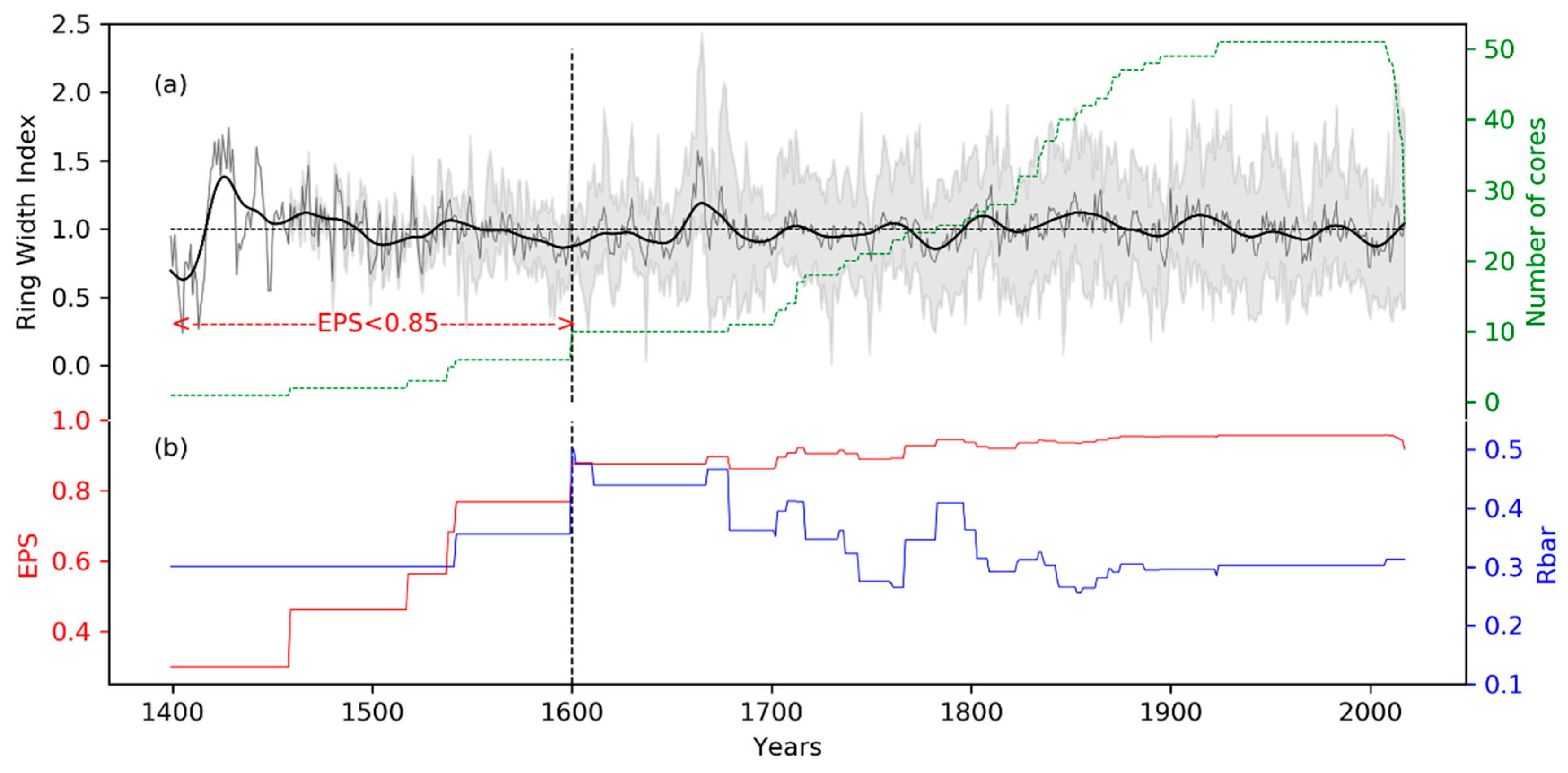
3.1. Ring Width Chronology

Our Timang ring-width chronology of T. dumosa covers 619 years, spanning from 1399 to 2017 CE (Figure 3). The average annual radial growth of trees is 0.927 mm, with a standard deviation of 0.327. The T. dumosa chronology shows a distinct variability in growth over the last six centuries, with a mean inter-series correlation of 0.474, indicating a strong common forcing by environmental parameters on tree growth. The EPS threshold of 0.85 was reached after 1600 CE when the chronology shows a replication with 10 cores (Figure 3a). Other important chronology statistics are displayed in Table 1.

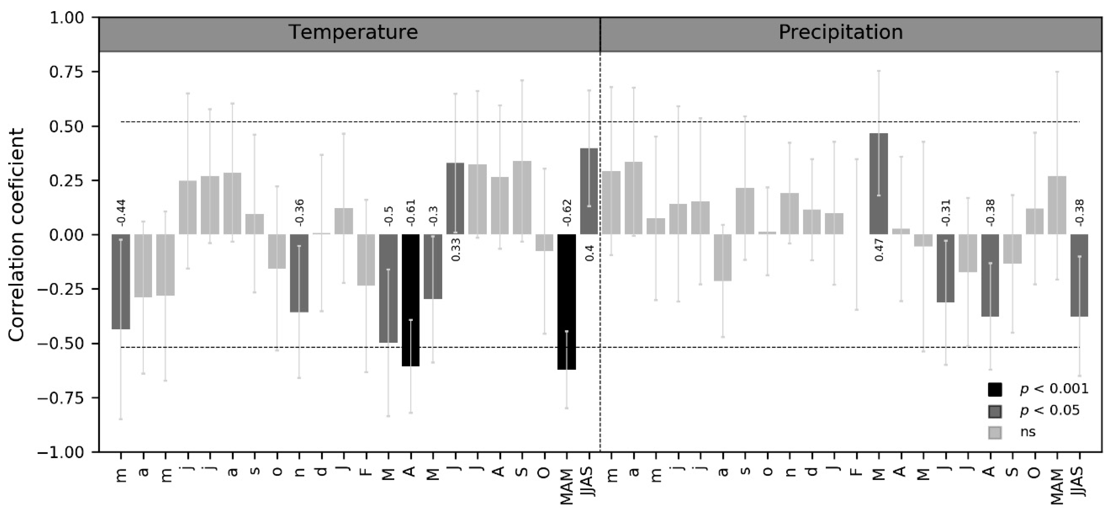
3.2. Relationship Between Radial Tree Growth and Climate

Correlation analyses between our TRW chronology and climate parameters (temperature and precipitation) from Chame station reveal significant (p < 0.05) negative correlations between the tree-ring chronology and March, April, and May temperatures and November (p < 0.05) temperature of the previous growth year. In contrast, a positive correlation occurs with the June temperature of the current year (Figure 4). On the other hand, growth correlated positively with precipitation in March, whereas correlations with current June and August were negative (Figure 4). The correlation of radial growth with seasonal temperatures revealed strong negative correlations for the spring (March–May) temperature (r = −0.62, p < 0.001), and positive correlations with the summer monsoon season (June–September) temperature (r = 0.40). In contrast, correlations with monsoon season precipitation were significantly negative (r = −0.38). The partial correlation analysis of spring temperature and precipitation meant that the correlation between the ring width and temperature was not strongly reduced under the exclusion of precipitation. On the other hand, there was a 48.5% reduction in the correlation with precipitation under the exclusion of temperature (Table 2).

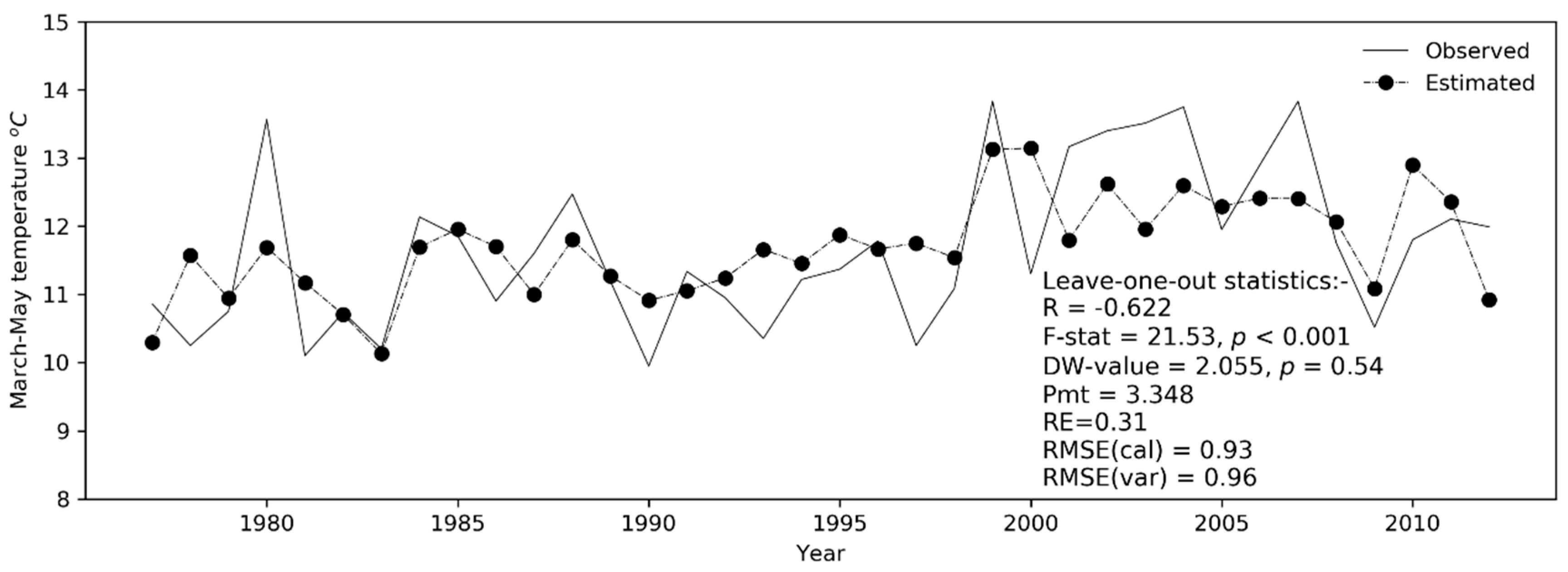
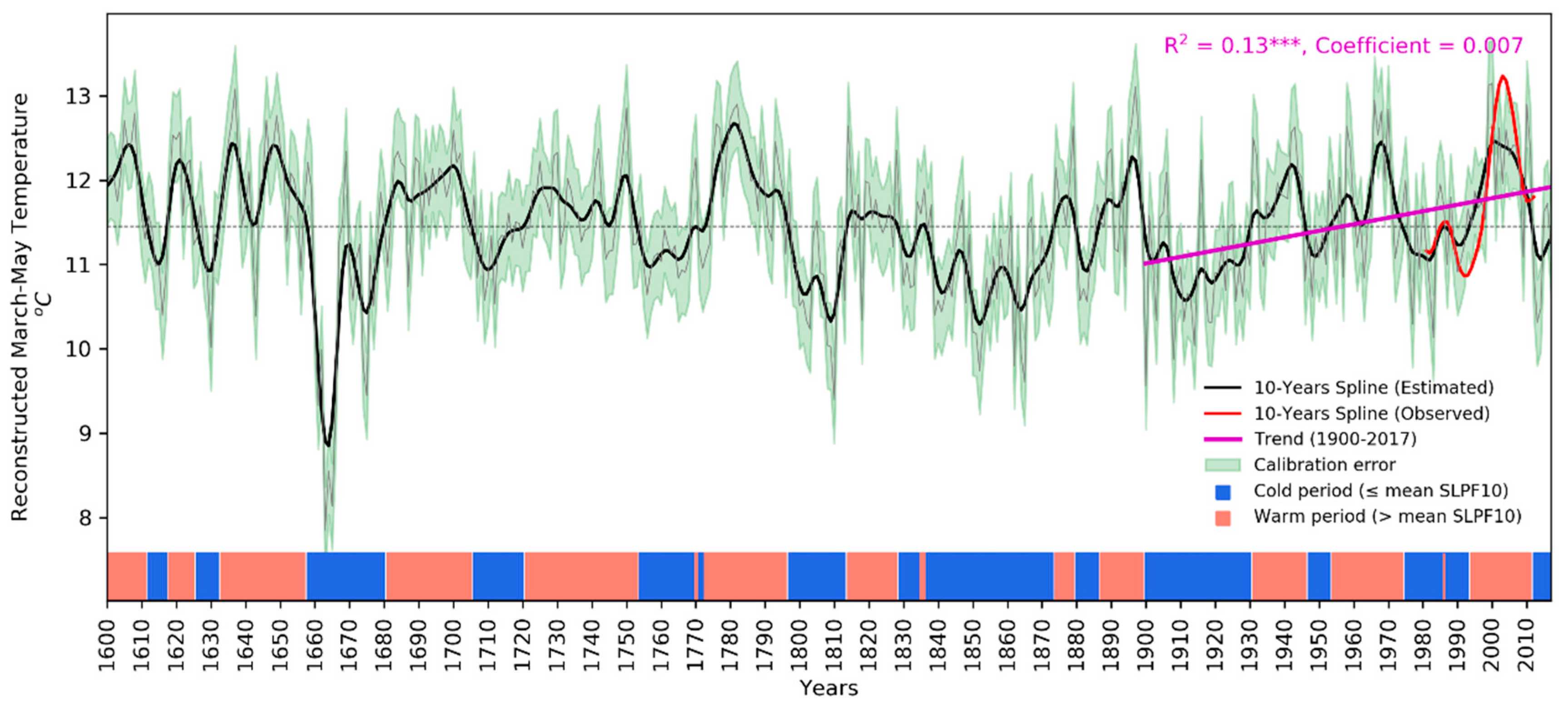
3.3. Spring Temperature Reconstruction

Based on the strongest response of the Timang Tsuga TRW-chronology with March–May temperatures, we reconstructed the spring temperature of the current growth season by applying a linear regression model and tested the robustness of the model with the ‘leave-one-out’ approach (Figure 5). The modeled temperature explained 38.7% of the variations of the actual spring temperature. The F-statistics value was 21.53, which is highly significant (p < 0.001). The model showed a positive value for the reduction of error (RE) (0.31) (Figure 5), indicating the robustness of the reconstruction [18,47]. The root mean square errors (RMSEs) for the calibration and verification periods were 0.93 and 0.96, respectively, which further underlines the robustness of the linear model. The Durbin–Watson statistics’ value was 2.0 (p = 0.54), indicating that the residuals of the regression model are free of autocorrelation (see the statistics of the model in Figure 5).
Using the linear model, a 418-year-long spring (March–May) temperature series was reconstructed, spanning from 1600 to 2017 CE. The reconstruction characteristics revealed an average temperature of 11.45 °C throughout the entire period of reconstruction (Figure 6). The maximum and minimum temperatures were 13.15 and 7.85 °C for 2000 CE and 1663 CE, respectively. Cool and warm periods over the whole reconstructed period are listed in Table 3 and shown in Figure 6b. The overall trend of the spring temperature increased at a rate of 0.07 °C per decade since the beginning of the 20th century (Figure 6).

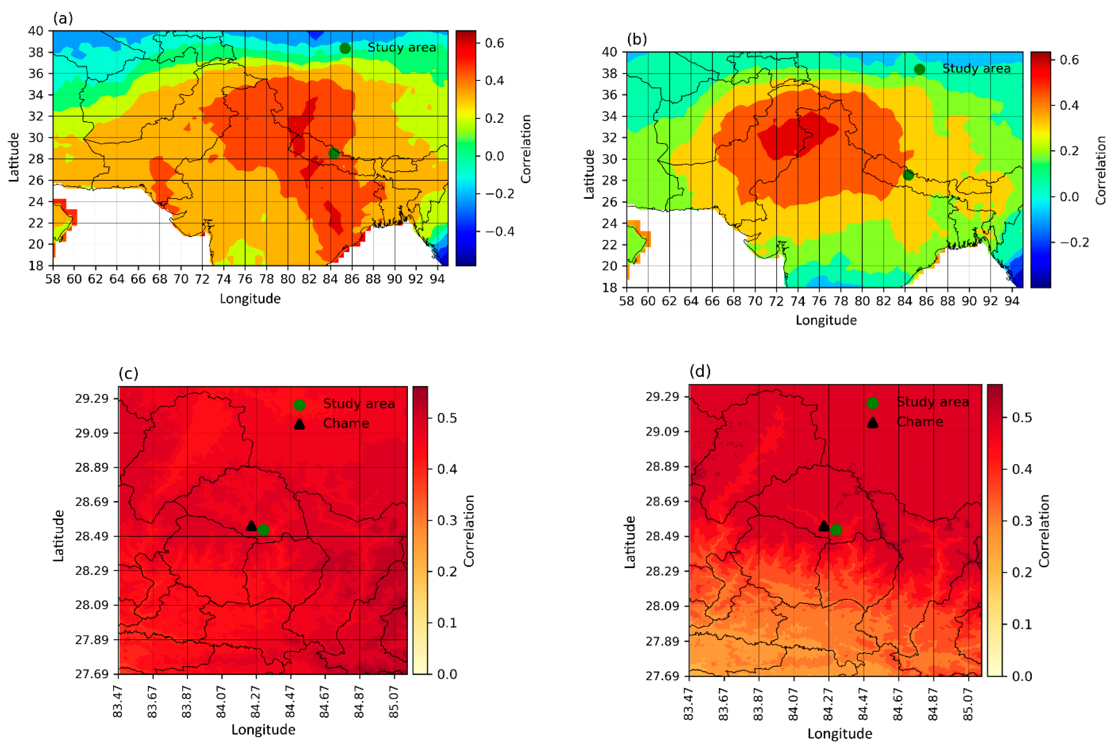
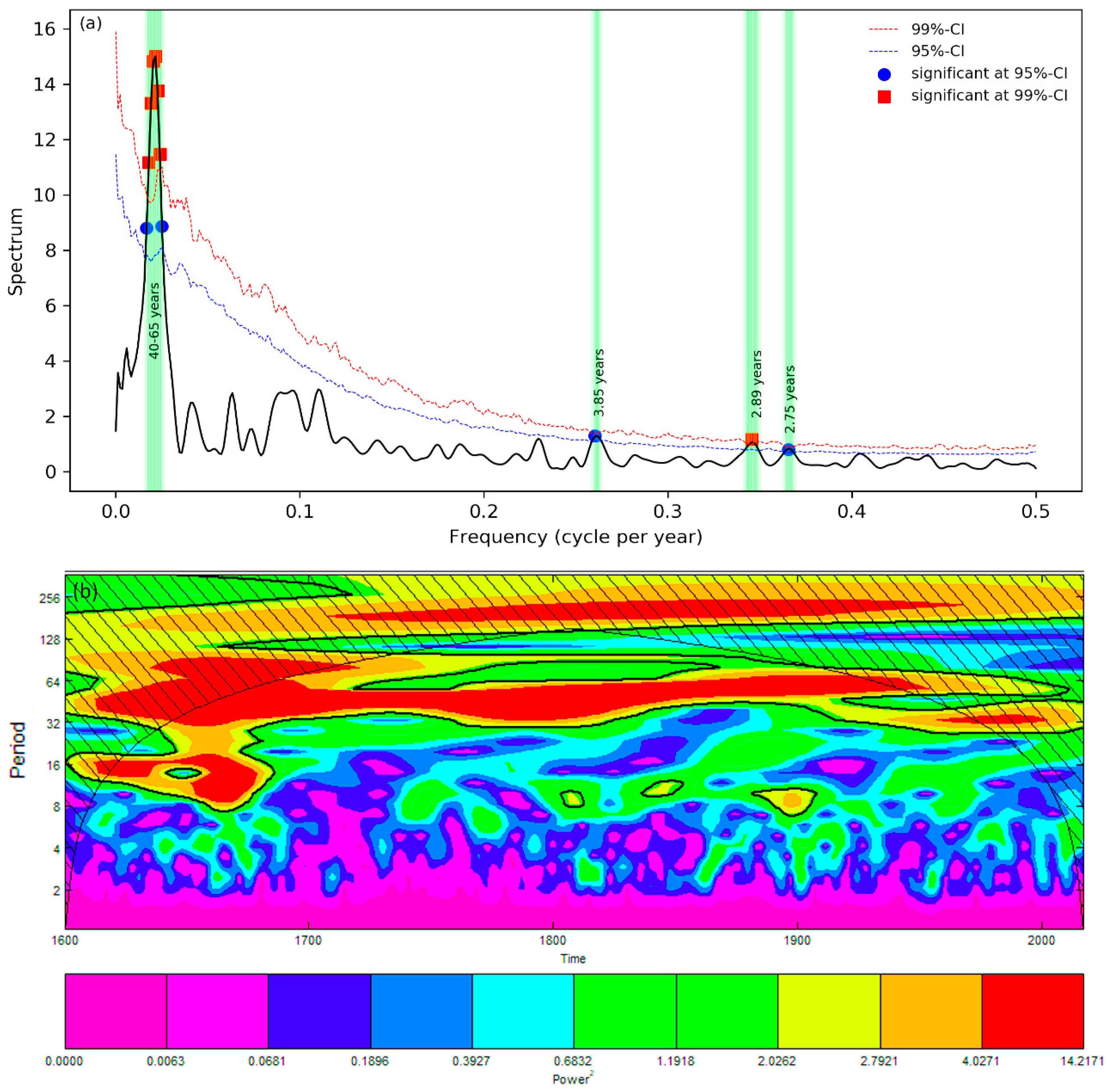
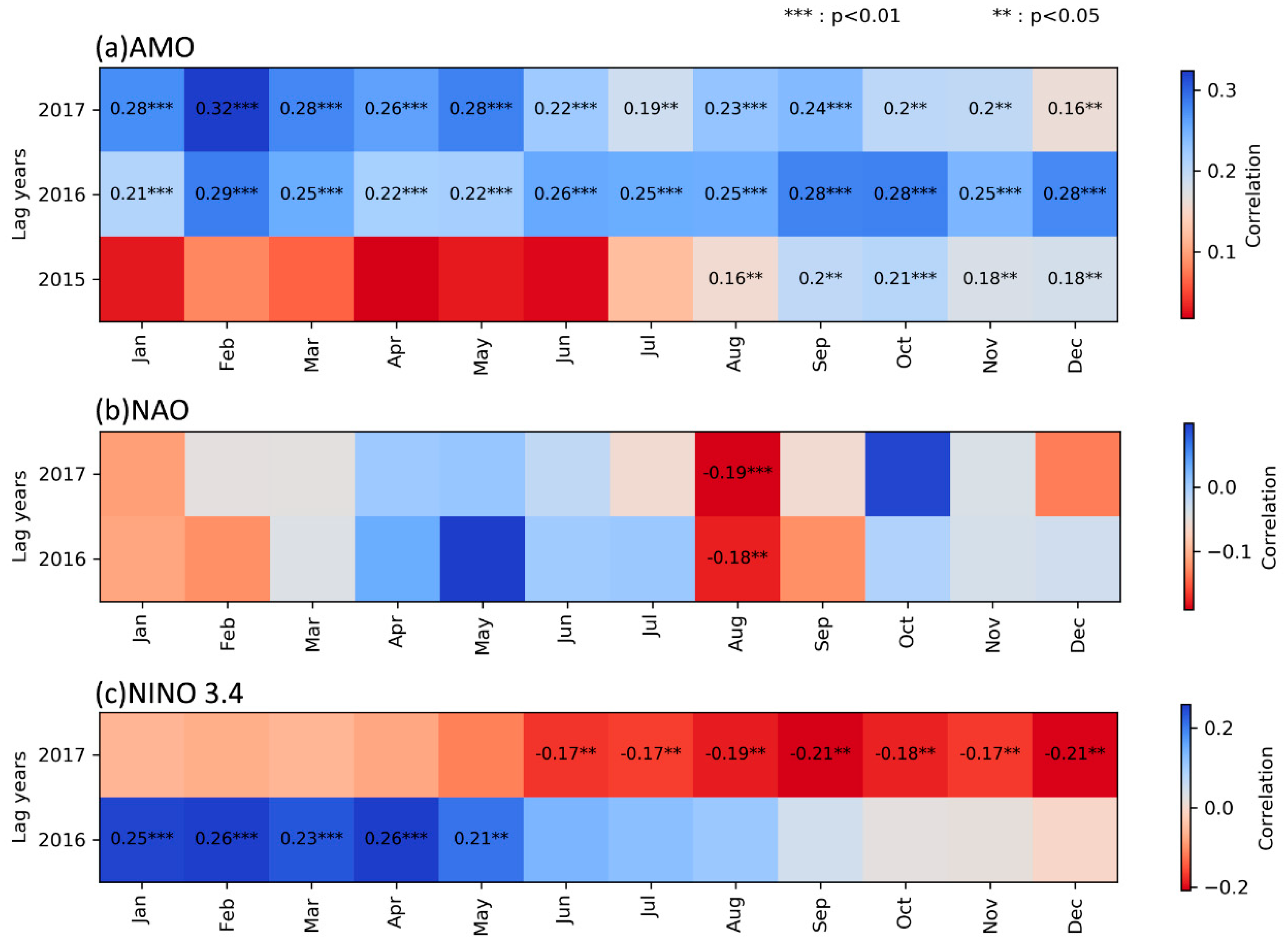
3.4. Spatial Coverage and Teleconnections of the Reconstructed Temperature Series

The reconstructed spring temperatures show strong positive relationships with March–May averaged CRU-gridded temperature data (Figure 7b). The relation was strongest for western Nepal and north-west India (Figure 7a,b). Similarly, CHELSA temperature data with a high spatial resolution of 1 square kilometer show significantly high correlations with the reconstructed temperature at our study site and 200 km around it (Figure 7c,d). Thus, our reconstructed temperature can be regarded as being representative of spring season temperature trends in the western to central Himalaya and neighboring regions.

4. Discussion

4.1. Characteristics of the Timang T. Dumosa Chronology

Nepal harbors many tree species with high dendroclimatic potential [19,20,21]. We built a 618-year-long ring-width chronology of T. dumosa from central Nepal, spanning the period from 1399 to 2017 CE. However, only for 1600–2017 CE, the EPS value was higher than the commonly used threshold value (0.85) [45]. The chronology statistics, the inter-series correlation, standard deviation, running Rbar, SNR, and mean sensitivity, lie within reported optimum levels [18,47]. The inter-series correlation and SNR for this study were higher compared to previous studies of the same species [21,33,34,35], indicating the robustness of our chronology. Similar to most of the tree-ring-width chronologies in Nepal [19,53,54], we also observed a significant growth depression during the 1810s, followed by a distinct increase in growth since 2003 CE. Thapa et al. [54] developed a composite chronology combining 55 tree chronologies from Nepal and mentioned these growth fluctuations as a major milestone for Nepalese tree-ring chronologies regardless of the tree species.
Our ring-width chronology indicates negative correlations with the March–May average temperature and positive relations with March rainfall, which is also considered as the spring season in Nepal. Most of the conifers in the high Himalaya show similar responses to the temperatures in the early growth period [15,19,23,24,26,55,56]. In the high Himalaya, broad-leaved species (Betula utilis D.Don) also show a negative response with spring temperature and a positive relationship with precipitation [53,57,58]. In the subtropical region of Nepal, conifers (Pinus roxburghii Sarg.) showed a similar negative response to spring temperature and positive to spring precipitation [59,60]. In the humid eastern Himalayan region in Sikkim and in Southwest China (Yunnan Province), T. dumosa showed a negative response to spring temperature and positive relationship of precipitation with the spring season [33,34,35,36]. Furthermore, various conifer species in northwest India showed a similar response with spring climate as in our study [61,62,63,64,65,66,67]. This climate–growth relation clearly indicates that there is an additive impact of temperature and precipitation during the spring season on the growth of T. dumosa. However, the partial correlation analysis (Table 2) shows that a great proportion (96.11%) of the correlation is from the temperature, which indicates that the mixed effect is primarily driven by high temperature. In Nepal, temperature increases rapidly after winter, whereas precipitation lags by some months (Figure 2b) because the heating of Tibetan Plateau is essential to trigger the onset of the Asian monsoon circulation [68]. This leads to warm and dry conditions before the onset of summer monsoon precipitation. These conditions create potential water deficits due to increasing evapotranspiration in these months [23,69,70]. Furthermore, the response of T. dumosa was positive with temperature and negative with precipitation during the summer monsoon season (June–September), with ample rainfall. This response is rather site-specific because of the inconsistent responses with the summer temperature and precipitation observed over Nepal. For instance, several studies from different locations in the Nepal Himalaya showed positive relationships with the summer (June–September) temperature and negative relationships with summer precipitation [26,38,71], whereas other studies showed the opposite response [27,29]. During the summer monsoon season, trees generally receive sufficient water; therefore, high temperatures during this period are conducive for photosynthesis and tree growth. An important fact to be considered in high elevations is that high precipitation implies a denser cloud cover, leading to a significant decrease in incoming solar radiation and to lower soil temperatures. This may ultimately retard tree growth [72] and may explain the negative relationships between radial growth and summer monsoon season rainfall at high-elevation sites.

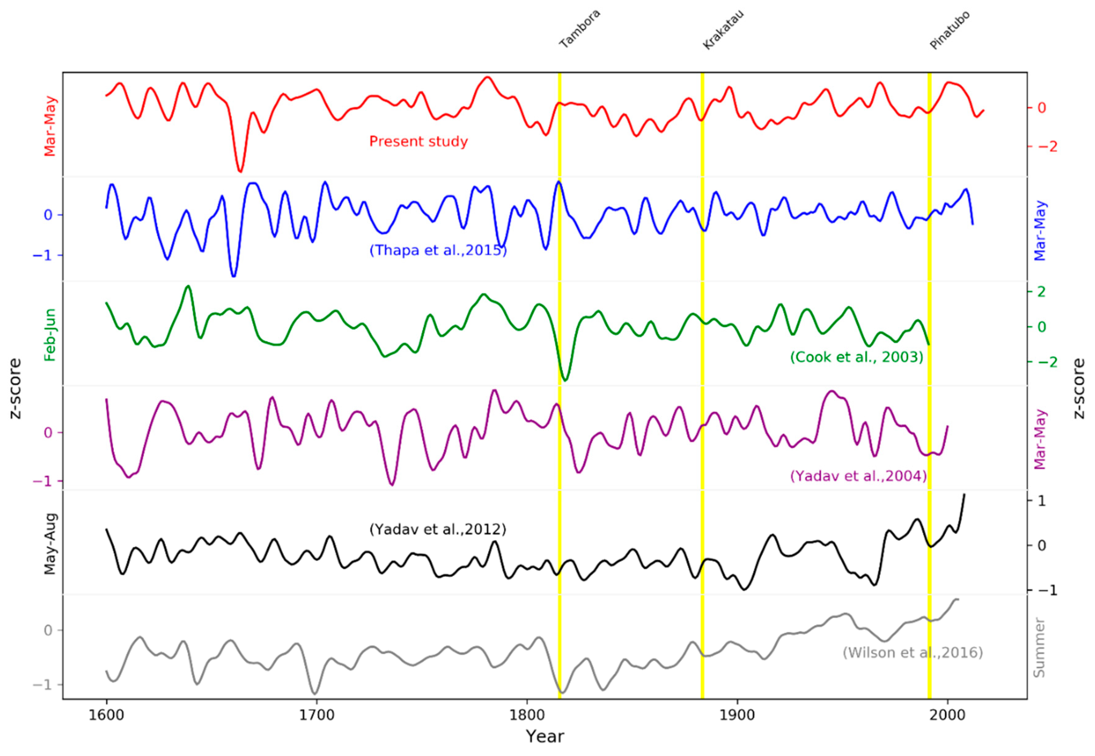
4.2. Long-Term Trend in Spring Temperature and Teleconnections

Our MAM temperature reconstruction showed different warm and cool episodes during the past 418 years. Some of the prominent cool episodes occurred in the 1660s, 1810s, 1880s, 1910s, and 1990s and some of them occurred contemporaneously with major volcanic eruptions (Figure 8). However, the superposed epoch analysis (SEA) did not show any significant effect of volcanic events on the reconstructed temperature (see Figure S1 in the Supplementary Materials). We compared our reconstructed temperature with other regional temperature reconstructions (Figure 8) and found a significant positive correlation (r = 0.23, p < 0.001) with a P. smithiana ring-width-based March–May temperature reconstruction from far-western Nepal by Thapa et al. [24]. The correlation of our temperature with the Februrary–June temperature series reconstructed by Cook et al. [19] was weak but showed higher coherency in low-frequency trends (after 30-year smoothing). We observed a sharp temperature depression during the 1660s, which is also present in the reconstruction of Thapa et al. [24] but absent in other reconstructions. This probably indicates an impact of local climate events or even of non-climatic events. The cool periods in the 1810s, 1880s, and 1910s were also observed in other reconstructions that may be associated with major volcanic eruptions in the tropical region (Figure 8). Although these cool periods during these volcanic eruptions coincide within the local and regional climate reconstructions, the magnitude of cooling differs. This clearly indicates that the local topography and orography are more dominant factors defining the climate in Himalaya. Individual impacts of different volcanic eruptions were reported in previous research [73], and it highlighted that a local tree-ring index should not be used as a direct indicator of volcanic forcing intensity. Studies linking recent volcanic eruptions of the 20th century to instrumental temperature data showed the possibility of differential effects depending on the geographical location (latitude), timing (season) of eruption, composition (sulphur content) of the volcanic gas, and the atmospheric circulation state in the particular year of the eruption (e.g., during El Niño years) [73,74,75,76]. The cold period at the beginning of the 20th century (1900–1936 CE) in our reconstruction reflects the coolest prolonged period in the study area for the last two centuries. Evidence from ice core and tree-ring data reported prolonged cooling at the beginning of 20th century and related this with climate fluctuations at the end of the ‘Little Ice Age’ [77,78,79]. Our reconstructed temperature series shows similar low frequency (multi-decadal) temperature variability with reconstructed temperatures of northwest India [65,80] and the Northern Hemisphere [81], especially during the 1820s, 1880s, and 1990s (Figure 8).
Our reconstruction captures spring temperature variations over a large spatial area of the central and western Himalayas and most parts of the Tibetan Plateau. The time span of instrumental climatic data in western Nepal is not long enough to contribute to CRU gridded data, which has a coarser (0.5°) spatial resolution (https://crudata.uea.ac.uk/cru/data/landstations/crustnsused.txt). That might be the major reason for the weaker correlations of our reconstructed temperature series with the grids closer to the study area. On the other hand, climate data from CHELSA are based on the topo-climate (e.g., orographic effect and wind fields) of small areas (~1 square kilometer resolution), so they better represent the local climatic conditions [50].
Spectral and wavelet analysis of the reconstructed temperature series indicated the presence of periodicities of 48 and 2.75 to 4 years (Figure 9a,b). The 2.75–4-year cycle could be associated with the El Niño Southern Oscillation (ENSO), which has a frequency of about 3–8 years [83]. The 40–65-year climate cycle may be related to the North Atlantic Oscillation (NAO) [84] or to the Atlantic Multi-decadal Oscillation (AMO) [85]. As discussed in previous studies, these climatic cycles have a major impact on the regional climate of Nepal [24,26,36,86]. We further calculated lagged correlation analysis to study the time lag between the occurrence of these climate modes and events and their impact on the climate of the Himalayan region (Figure 10). Our temperature reconstruction showed a positive correlation with the AMO of every month of the current and previous year, implying that AMO has a significant impact on the growth of trees in our study area. Previous studies found that a positive AMO mode extends the duration of the summer monsoon in the southeast and east Asia [87]. Li et al. [85] claimed that the East Asian temperature leads to the occurrence of the positive AMO phase, which creates a positive relationship with temperature and AMO. The effect of the positive NAO index is negative on spring temperature (favoring growth) in our study area. Li et al. [88] reported a positive effect of winter NAO on the spring growth of vegetation in the entire Eurasia. In Asia, a positive winter NAO results in increased temperature, precipitation, and soil moisture during the winter season, accumulating a thin snow cover during spring [88]. The moist soil and early snowmelt provide more moisture favoring plant growth in the spring season. Similarly, previous year January–May El Niño sea surface temperature (SST) (NINO3.4) also has a positive correlation with the reconstructed temperature. The El Niño phenomenon is not only responsible for controlling temperature variations in the equatorial Pacific region but also has an impact on extratropical circulation [89]. High NINO3.4 region SSTs cause warm winters that peak in the following spring season and delays the onset of the Indian Summer Monsoon (ISM), which causes a prolonged hot and dry spring season in Southeast Asia [90,91].

5. Conclusions

We present a new six-century-long chronology of T. dumosa from western Nepal, which showed a strong negative signal to spring (March–May) temperature, consistent with other chronologies from the region. This signal provided the basis to develop the first spring temperature reconstruction for the last four centuries in the Trans-Himalayan region of Nepal. Our new spring temperature reconstruction revealed various warm and cool episodes and a significant warming trend since the beginning of the 20th century, although previous periods had experienced similarly warm episodes. Unlike other regional or global temperature reconstructions, our reconstruction did not show any significant increasing term trend over the last four centuries. The effects of volcanic forcing in the temperature trend in the central Himalayas are not perfectly synchronized between reconstructions from different locations, but some of the cool periods in the reconstructed temperature records coincide with major volcanic eruptions while others do not. This indicates that the local topography and orography effects play a strongly modifying role for temperature variations in the Himalaya on large-scale climatic effects, like, e.g., volcanic forcing. The reconstructed spring temperature series contained periodicities that coincide with the periodicity of broader scale climate modes, such as AMO, NAO, and ENSO. This implies that the temperature in our study area is also regulated by broad-scale atmospheric circulation patterns.

Supplementary Materials

The following are available online at https://www.mdpi.com/2073-4433/11/2/132/s1, Figure S1: Result of Superposed Epoch Analysis of volcanic events in 1815, 1883 and 1991 on reconstructed temperature, Figure S2: Relation of chronology with CRU-TS averaged temperature and precipitation of four grids around study area, Figure S3: Correlation of chronology with maximum and minimum temperature of study area, Figure S4: Correlation of chronology with the climate after removing autocorrelation using 1st difference, Figure S5: Running correlation between reconstructed temperatures by Thapa et al. [24] and in our study, Table S1: Comparison of chronology statistics of different detrending methods, Table S2: Leave-one-out calbration and verification statistics using diffrent detrending methods with Mar-May temperature.

Author Contributions

Conceptualization: N.P.G., S.A., and P.R.; field and laboratory work: N.P.G., S.A., P.R., N.R.P., B.S.; data analysis and interpretation; S.A., N.P.G., N.D. and J.G.; methodology, writing and original draft preparation: all authors; funding acquisition: N.P.G. and A.B. All authors have read and agreed to the published version of the manuscript.

Funding

This research was supported by project titled “Biogeographical aspects of climatic stress resilience of mountain forests of the central Himalaya” funded by Alexander von Humboldt Foundation, and Yunnan Oriented Fund for Post Doctors and ‘The CAS President’s International Fellowship Initiative’ (PIFI) postdoctoral fellowship (2019PC0102) for N.P.G.

Acknowledgments

We express our sincere gratitude to the Department of National Park and Wildlife Conservation, Annapurna Conservation Area for permitting this study in conservation area. We would also like to thank the Department of Hydrology and Meteorology (DHM) of Nepal for providing meteorological data. We are grateful to the people of Timang village for their hospitality and support during sampling.

Conflicts of Interest

The authors declare no conflict of interest.

References

  1. Shrestha, A.B.; Aryal, R. Climate change in Nepal and its impact on Himalayan glaciers. Reg. Environ. Chang. 2011, 11, 65–77. [Google Scholar] [CrossRef]
  2. Xu, J.; Grumbine, R.E.; Shrestha, A.; Eriksson, M.; Yang, X.; Wang, Y.; Wilkes, A. The Melting Himalayas: Cascading Effects of Climate Change on Water, Biodiversity, and Livelihoods. Conserv. Biol. 2009, 23, 520–530. [Google Scholar] [CrossRef]
  3. Climate Change, Glacier Response, and Vegetation Dynamics in the Himalaya: Contributions Toward Future Earth Initiatives; Singh, R.B.; Schickhoff, U.; Mal, S. (Eds.) Springer International Publishing: Cham, Germany, 2016; ISBN 978-3-319-28977-9. [Google Scholar]
  4. Shrestha, U.B.; Shrestha, A.M.; Aryal, S.; Shrestha, S.; Gautam, M.S.; Ojha, H. Climate change in Nepal: A comprehensive analysis of instrumental data and people’s perceptions. Clim. Chang. 2019, 61, 477. [Google Scholar] [CrossRef]
  5. Pepin, N.; Bradley, R.S.; Diaz, H.F.; Baraer, M.; Caceres, E.B.; Forsythe, N.; Fowler, H.; Greenwood, G.; Hashmi, M.Z.; Liu, X.D.; et al. Elevation-dependent warming in mountain regions of the world. Nat. Clim. Chang. 2015, 5, 424–430. [Google Scholar] [CrossRef] [Green Version]
  6. IPCC. Climate Change 2007. Synthesis Report. Contribution of Working Groups I, II and III to the Fourth Assessment Report of the Intergovernmental Panel on Climate Change; Cambridge University Press: Cambridge, UK; New York, NY, USA, 2007; ISBN 92-9169-122-4. [Google Scholar]
  7. IPCC. International Panel of Climate Change. Climate Change 2013: The Physical Science Basis. Contribution of Working Group I to the Fifth Assessment Report of the Intergovernmental Panel on Climate Change; Cambridge University Press: Cambridge, UK; New York, NY, USA, 2013. [Google Scholar] [CrossRef] [Green Version]
  8. Talchabhadel, R.; Karki, R.; Thapa, B.R.; Maharjan, M.; Parajuli, B. Spatio-temporal variability of extreme precipitation in Nepal. Int. J. Climatol. 2018, 38, 4296–4313. [Google Scholar] [CrossRef]
  9. Rangwala, I.; Miller, J.R. Climate change in mountains: A review of elevation-dependent warming and its possible causes. Clim. Chang. 2012, 114, 527–547. [Google Scholar] [CrossRef]
  10. Gottfried, M.; Pauli, H.; Futschik, A.; Akhalkatsi, M.; Barančok, P.; Benito Alonso, J.L.; Coldea, G.; Dick, J.; Erschbamer, B.; Fernández Calzado, M.R.; et al. Continent-wide response of mountain vegetation to climate change. Nat. Clim. Chang. 2012, 2, 111–115. [Google Scholar] [CrossRef]
  11. Theurillat, J.-P.; Guisan, A. Potential impact of climate change on vegetation in the European Alps: A review. Clim. Chang. 2001, 50, 77–109. [Google Scholar] [CrossRef]
  12. Ziaco, E.; Biondi, F.; Rossi, S.; Deslauriers, A. Climatic influences on wood anatomy and tree-ring features of Great Basin conifers at a new mountain observatory. Appl. Plant Sci. 2014, 2. [Google Scholar] [CrossRef]
  13. Gaire, N.P.; Koirala, M.; Bhuju, D.R.; Borgaonkar, H.P. Treeline dynamics with climate change at the central Nepal Himalaya. Clim. Past 2014, 10, 1277–1290. [Google Scholar] [CrossRef] [Green Version]
  14. Carrer, M.; Brunetti, M.; Castagneri, D. The Imprint of Extreme Climate Events in Century-Long Time Series of Wood Anatomical Traits in High-Elevation Conifers. Front. Plant Sci. 2016, 7, 683. [Google Scholar] [CrossRef] [Green Version]
  15. Gaire, N.P.; Koirala, M.; Bhuju, D.R.; Carrer, M. Site- and species-specific treeline responses to climatic variability in eastern Nepal Himalaya. Dendrochronologia 2017, 41, 44–56. [Google Scholar] [CrossRef]
  16. Department of Hydrology and Meteorology. Observed Climate Trend Analysis of Nepal (1971–2014); Department of Hydrology and Meteorology: Kathmandu, Nepal, 2017. Available online: https://www.dhm.gov.np/uploads/climatic/467608975Observed%20Climate%20Trend%20Analysis%20Report_2017_Final.pdf (accessed on 5 September 2019).
  17. Shrestha, U.B.; Gautam, S.; Bawa, K.S. Widespread climate change in the Himalayas and associated changes in local ecosystems. PLoS ONE 2012, 7, e36741. [Google Scholar] [CrossRef] [Green Version]
  18. Speer, J.H. Fundamentals of Tree-Ring Research; The University of Arizona Press: Tucson, Arizona, 2010; ISBN 978-0-8165-2684-0. [Google Scholar]
  19. Cook, E.R.; Krusic, P.J.; Jones, P.D. Dendroclimatic Signals in Long Tree-Ring Chronologies from the Himalayas of Nepal. Int. J. Climatol. 2003, 23, 26–29. [Google Scholar] [CrossRef]
  20. Gaire, N.P.; Bhuju, D.R.; Koirala, M. Dendrochronological studies in nepal: Current status and future prospects. FUUAST J. Biol. 2013, 3, 1–9. [Google Scholar]
  21. Bhattacharyya, A.; Lamarche, V.C.; Hughes, M.K. Tree -ring chronologies from Nepal. Tree-Ring Bull. 1992, 52, 59–66. [Google Scholar]
  22. Esper, J.; Schweingruber, F.H.; Winiger, M. 1300 years of climatic history for Western Central Asia inferred from tree-rings. Holocene 2002, 12, 267–277. [Google Scholar] [CrossRef] [Green Version]
  23. Sano, M.; Furuta, F.; Kobayashi, O.; Sweda, T. Temperature variations since the mid-18th century for western Nepal, as reconstructed from tree-ring width and density of Abies spectabilis. Dendrochronologia 2005, 23, 83–92. [Google Scholar] [CrossRef]
  24. Thapa, U.K.; Shah, S.K.; Gaire, N.P.; Bhuju, D.R. Spring temperatures in the far-western Nepal Himalaya since AD 1640 reconstructed from Picea smithiana tree-ring widths. Clim. Dyn. 2015, 45, 2069–2081. [Google Scholar] [CrossRef]
  25. Sano, M.; Ramesh, R.; Sheshshayee, M.S.; Sukumar, R. Increasing aridity over the past 223 years in the Nepal Himalaya inferred from a tree-ring δ18O chronology. Holocene 2011, 22, 809–817. [Google Scholar] [CrossRef]
  26. Gaire, N.P.; Bhuju, D.R.; Koirala, M.; Shah, S.K.; Carrer, M.; Timilsena, R. Tree-ring based spring precipitation reconstruction in western Nepal Himalaya since AD 1840. Dendrochronologia 2017, 42, 21–30. [Google Scholar] [CrossRef]
  27. Panthi, S.; Bräuning, A.; Zhoua, Z.-K.; Fan, Z.-X. Tree rings reveal recent intensified spring drought in the central Himalaya, Nepal. Glob. Planet. Chang. 2017, 157, 26–34. [Google Scholar] [CrossRef]
  28. Bhandari, S.; Gaire, N.P.; Shah, S.K.; Speer, J.H.; Bhuju, D.R.; Thapa, U.K. A 307-year tree-ring SPEI reconstruction indicates modern drought in western Nepal Himalayas. Tree-Ring Res. 2019, 75, 73–85. [Google Scholar] [CrossRef]
  29. Gaire, N.P.; Dhakal, Y.R.; Shah, S.K.; Fan, Z.-X.; Bräuning, A.; Thapa, U.K.; Bhandari, S.; Aryal, S.; Bhuju, D.R. Drought (scPDSI) reconstruction of trans-Himalayan region of central Himalaya using Pinus wallichiana tree-rings. Palaeogeogr. Palaeoclimatol. Palaeoecol. 2019, 514, 251–264. [Google Scholar] [CrossRef]
  30. Karki, R.; Talchabhadel, R.; Aalto, J.; Baidya, S.K. New climatic classification of Nepal. Theor. Appl. Climatol. 2016, 125, 799–808. [Google Scholar] [CrossRef]
  31. Farjon, A. A Handbook of the World’s Conifers (2 vols.); Brill: Leiden, The Netherlands, 2010; ISBN 978-90-47-43062-9. [Google Scholar]
  32. Havill, N.P.; Campbell, C.S.; Vining, T.F.; LePage, B.; Bayer, R.J.; Donoghue, M.J. Phylogeny and Biogeography of Tsuga (Pinaceae) Inferred from Nuclear Ribosomal ITS and Chloroplast DNA Sequence Data. Syst. Bot. 2008, 33, 478–489. [Google Scholar] [CrossRef]
  33. Fan, Z.-X.; Bräuning, A.; Cao, K.-F. Tree-ring based drought reconstruction in the central Hengduan Mountains region (China) since A.D. 1655. Int. J. Climatol. 2008, 28, 1879–1887. [Google Scholar] [CrossRef]
  34. Guo, G.; Zong-Shan, L.; Qi-Bin, Z.; Ke-Ping, M.; Conglong, M. Dendroclimatological studies of Picea likiangensis and Tsuga dumosa in Lijiang, China. IAWA J. 2009, 30, 435–441. [Google Scholar] [CrossRef] [Green Version]
  35. Jiang, Y.-m.; Li, Z.-S.; Fan, Z.-X. Tree-ring based February–April relative humidity reconstruction since A.D. 1695 in the Gaoligong Mountains, southeastern Tibetan Plateau. Asian Geogr. 2017, 34, 59–70. [Google Scholar] [CrossRef]
  36. Borgaonkar, H.P.; Gandhi, N.; Ram, S.; Krishnan, R. Tree-ring reconstruction of late summer temperatures in northern Sikkim (eastern Himalayas). Palaeogeogr. Palaeoclim. Palaeoecol. 2018, 504, 125–135. [Google Scholar] [CrossRef]
  37. NTNC. National Trust for Nature Conservation, Annual Report December; National Trust for Nature Conservation: Lalitpur, Nepal, 2015. [Google Scholar]
  38. Kharal, D.K.; Thapa, U.K.; St George, S.; Meilby, H.; Rayamajhi, S.; Bhuju, D.R. Tree-climate relations along an elevational transect in Manang Valley, central Nepal. Dendrochronologia 2017, 41, 57–64. [Google Scholar] [CrossRef]
  39. Rinn, F. TSAP-WIN: Time Series Analysis and Presentation Dendrochonology and Related Applications; RINNTECH: Heidelberg, Germany, 2013. [Google Scholar]
  40. Holmes, R.L. Computer-assisted quality control in Tree-ring dating and measurement. Tree-Ring Bull. 1983, 43, 69–78. [Google Scholar]
  41. Grissino-Mayer, H.D. Evaluating crossdating accuracy: A manual and tutorial for the computer program COFECHA. Tree-Ring Res. 2001, 57, 17. [Google Scholar]
  42. Cook, E.R. A time series analysis approach to tree ring standardization. Doctoral Dissertation, University of Arizona, Tucson, AZ, USA.
  43. Bunn, A.G. A dendrochronology program library in R (dplR). Dendrochronologia 2008, 26, 115–124. [Google Scholar] [CrossRef]
  44. R Development Core Team. R: A language and environment for statistical computing; R Foundation for Statistical Computing: Vienna, Austria, 2019. [Google Scholar]
  45. Wigley, T.M.L.; Briffa, K.R.; Jones, P.D. On the Average Value of Correlated Time Series, with Applications in Dendroclimatology and Hydrometeorology. J. Clim. Appl. Meteorol. 1984, 23, 201–213. [Google Scholar] [CrossRef]
  46. Zang, C.; Biondi, F. treeclim: An R package for the numerical calibration of proxy-climate relationships. Ecography 2015, 38, 431–436. [Google Scholar] [CrossRef]
  47. Fritts, H.C. Tree Rings and Climate; Academic Press: New York, NY, USA, 1976; ISBN 0-12-268450-8. [Google Scholar]
  48. Michaelsen, J. Cross-Validation in Statistical Climate Forecast Models. J. Clim. Appl. Meteorol. 1987, 26, 1589–1600. [Google Scholar] [CrossRef] [Green Version]
  49. Esper, J.; Frank, D.; Büntgen, U.; Verstege, A.; Luterbacher, J.; Xoplaki, E. Long-term drought severity variations in Morocco. Geophys. Res. Lett. 2007, 34, 2929. [Google Scholar] [CrossRef] [Green Version]
  50. Karger, D.N.; Conrad, O.; Böhner, J.; Kawohl, T.; Kreft, H.; Soria-Auza, R.W.; Zimmermann, N.E.; Linder, H.P.; Kessler, M. Climatologies at high resolution for the earth’s land surface areas. Sci. Data 2017, 4, 170122. [Google Scholar] [CrossRef] [Green Version]
  51. Torrence, C.; Compo, G.P. A Practical Guide to Wavelet Analysis. Bull. Am. Meteorol. Soc. 1998, 79, 61–78. [Google Scholar] [CrossRef] [Green Version]
  52. Schulz, M.; Mudelsee, M. REDFIT: Estimating Red-noise Spectra Directly from Unevenly Spaced Paleoclimatic Time Series. Comput. Geosci. 2002, 28, 421–426. [Google Scholar] [CrossRef]
  53. Liang, E.; Dawadi, B.; Pederson, N.; Eckstein, D. Is the growth of birch at the upper timberline in the Himalayas limited by moisture or by temperature? Ecology 2014, 95, 2453–2465. [Google Scholar] [CrossRef] [Green Version]
  54. Thapa, U.K.; St George, S.; Kharal, D.K.; Gaire, N.P. Tree growth across the Nepal Himalaya during the last four centuries. Prog. Phys. Geogr. 2017, 41, 478–495. [Google Scholar] [CrossRef]
  55. Thapa, U.K.; Shah, S.K.; Gaire, N.P.; Bhuju, D.R.; Bhattacharya, A.; Thagunna, G.S. Influence of climate on radial growth of Abiea pindrow in western Nepal Himalaya. Banko Janakari 2013, 23, 6. [Google Scholar]
  56. Tiwari, A.; Fan, Z.-X.; Jump, A.S.; Li, S.-F.; Zhou, Z.-K. Gradual expansion of moisture sensitive Abies spectabilis forest in the Trans-Himalayan zone of central Nepal associated with climate change. Dendrochronologia 2017, 41, 34–43. [Google Scholar] [CrossRef]
  57. Dawadi, B.; Liang, E.; Tian, L.; Devkota, L.P.; Yao, T. Pre-monsoon precipitation signal in tree rings of timberline Betula utilis in the central Himalayas. Quat. Int. 2013, 283, 72–77. [Google Scholar] [CrossRef]
  58. Tiwari, A.; Fan, Z.-X.; Jump, A.S.; Zhou, Z.-K. Warming induced growth decline of Himalayan birch at its lower range edge in a semi-arid region of Trans-Himalaya, central Nepal. Plant Ecol. 2017, 218, 621–633. [Google Scholar] [CrossRef]
  59. Aryal, S.; Bhuju, D.R.; Kharal, D.K.; Gaire, N.P.; Dyola, N. Climatic upshot using growth pattern of Pinus roxburghii from western Nepal. Pak. J. Bot. 2018, 50, 579–588. [Google Scholar]
  60. Sigdel, S.; Dawadi, B.; Camarero, J.; Liang, E.; Leavitt, S. Moisture-Limited Tree Growth for a Subtropical Himalayan Conifer Forest in Western Nepal. Forests 2018, 9, 340. [Google Scholar] [CrossRef] [Green Version]
  61. Yadav, R.R.; Park, W.-K.; Bhattacharyya, A. Dendroclimatic Reconstruction of April–May Temperature Fluctuations in the Western Himalaya of India Since A.D. 1698. Quat. Res. 1997, 48, 187–191. [Google Scholar] [CrossRef]
  62. Borgaonkar, H.P.; Pant, G.B.; Kumar, K.R. Tree-Ring Chronologies from Western Himalaya and Their Dendroclimatic Potential. IAWA J. 1999, 20, 295–309. [Google Scholar] [CrossRef]
  63. Yadav, R.R.; Park, W.K.; Bhattacharyya, A. Spring-temperature variations in western Himalaya, India, as reconstructed from tree-rings: AD 1390–1987. Holocene 1999, 9, 85–90. [Google Scholar] [CrossRef]
  64. Yadav, R.R.; Singh, J. Tree-Ring-Based Spring Temperature Patterns over the Past Four Centuries in Western Himalaya. Quat. Res. 2002, 57, 299–305. [Google Scholar] [CrossRef]
  65. Yadav, R.R.; Park, W.-K.; Singh, J.; Dubey, B. Do the western Himalayas defy global warming? Geophys. Res. Lett. 2004, 31. [Google Scholar] [CrossRef]
  66. Shah, S.K.; Shekhar, M.; Bhattacharyya, A. Anomalous distribution of Cedrus deodara and Pinus roxburghii in Parbati valley, Kullu, Western Himalaya: An assessment in dendroecological perspective. Quat. Int. 2014, 325, 205–212. [Google Scholar] [CrossRef]
  67. Sohar, K.; Altman, J.; Lehečková, E.; Doležal, J. Growth-climate relationships of Himalayan conifers along elevational and latitudinal gradients. Int. J. Climatol. 2017, 37, 2593–2605. [Google Scholar] [CrossRef]
  68. Böhner, J. General climatic controls and topoclimatic variations in Central and High Asia. Boreas 2006, 35, 279–295. [Google Scholar] [CrossRef]
  69. Borgaonkar, H.P.; Pant, G.B.; Kumar, K.R. Ring-width variations in Cedrus deodara and its climatic response over the western Himalaya. Int. J. Climatol. 1996, 16, 1409–1422. [Google Scholar] [CrossRef]
  70. Shrestha, K.B.; Hofgaard, A.; Vandvik, V. Tree-growth response to climatic variability in two climatically contrasting treeline ecotone areas, central Himalaya, Nepal. Can. J. For. Res. 2015, 45, 1643–1653. [Google Scholar] [CrossRef]
  71. Chhetri, P.K.; Cairns, D.M. Dendroclimatic response of Abies spectabilis at treeline ecotone of Barun Valley, eastern Nepal Himalaya. J. For. Res. 2016, 27, 1163–1170. [Google Scholar] [CrossRef]
  72. Takahashi, K.; Tokumitsu, Y.; Yasue, K. Climatic factors affecting the tree-ring width of Betula ermanii at the timberline on Mount Norikura, central Japan. Ecol. Res. 2005, 20, 445–451. [Google Scholar] [CrossRef] [Green Version]
  73. Jones, P.D.; Briffa, K.R.; Schweingruber, F.H. Treering evidence of the widespread effects of explosive volcanic eruptions. Geophys. Res. Lett. 1995, 22, 1333–1336. [Google Scholar] [CrossRef] [Green Version]
  74. Robock, A.; Mao, J. The Volcanic Signal in Surface Temperature Observations. J. Clim. 1995, 8, 1086–1103. [Google Scholar] [CrossRef] [Green Version]
  75. Anchukaitis, K.J.; Buckley, B.M.; Cook, E.R.; Cook, B.I.; D’Arrigo, R.D.; Ammann, C.M. Influence of volcanic eruptions on the climate of the Asian monsoon region. Geophys. Res. Lett. 2010, 37. [Google Scholar] [CrossRef]
  76. Li, M.; Huang, L.; Yin, Z.-Y.; Shao, X. Temperature reconstruction and volcanic eruption signal from tree-ring width and maximum latewood density over the past 304 years in the southeastern Tibetan Plateau. Int. J. Biometeorol. 2017, 61, 2021–2032. [Google Scholar] [CrossRef]
  77. Rowan, A.V. The ‘Little Ice Age’ in the Himalaya: A review of glacier advance driven by Northern Hemisphere temperature change. Holocene 2017, 27, 292–308. [Google Scholar] [CrossRef]
  78. Yang, B.; Bräuning, A.; Liu, J.; Davis, M.E.; Yajun, S. Temperature changes on the Tibetan Plateau during the past 600 years inferred from ice cores and tree rings. Global Planet. Chang. 2009, 69, 71–78. [Google Scholar] [CrossRef]
  79. Bräuning, A. Tree-ring evidence of ‘Little Ice Age’ glacier advances in southern Tibet. Holocene 2006, 16, 369–380. [Google Scholar] [CrossRef]
  80. Yadav, R.R.; Braeuning, A.; Singh, J. Tree ring inferred summer temperature variations over the last millennium in western Himalaya, India. Clim. Dyn. 2012, 36, 1545–1554. [Google Scholar] [CrossRef]
  81. Wilson, R.; Anchukaitis, K.; Briffa, K.R.; Büntgen, U.; Cook, E.; D’Arrigo, R.; Davi, N.; Esper, J.; Frank, D.; Gunnarson, B.; et al. Last millennium northern hemisphere summer temperatures from tree rings: Part I: The long term context. Quat. Sci. Rev. 2016, 134, 1–18. [Google Scholar] [CrossRef] [Green Version]
  82. Briffa, K.R.; Jones, P.D.; Schweingruber, F.H.; Osborn, T.J. Influence of volcanic eruptions on Northern Hemisphere summer temperature over the past 600 years. Nature 1998, 393, 450–455. [Google Scholar] [CrossRef]
  83. Yuan, Y.; Yang, S. Impacts of Different Types of El Niño on the East Asian Climate: Focus on ENSO Cycles. J. Clim. 2012, 25, 7702–7722. [Google Scholar] [CrossRef]
  84. Schlesinger, M.E.; Ramankutty, N. Low-frequency oscillation. Nature 1994, 372, 508–509. [Google Scholar] [CrossRef]
  85. Li, S.; Jing, Y.; Luo, F. The potential connection between China surface air temperature and the Atlantic Multidecadal Oscillation (AMO) in the Pre-industrial Period. Sci. China Earth Sci. 2015, 58, 1814–1826. [Google Scholar] [CrossRef]
  86. Bhattacharyya, A.; Yadav, R.R. Climatic reconstructions using tree-ring data from tropical and temperate regions of India -A review. IAWA J. 1999, 20, 311–316. [Google Scholar] [CrossRef]
  87. Lu, R.; Dong, B.; Ding, H. Impact of the Atlantic Multidecadal Oscillation on the Asian summer monsoon. Geophys. Res. Lett. 2006, 33, L08705. [Google Scholar] [CrossRef] [Green Version]
  88. Li, J.; Fan, K.; Xu, Z. Links between the late wintertime North Atlantic Oscillation and springtime vegetation growth over Eurasia. Clim. Dyn. 2016, 46, 987–1000. [Google Scholar] [CrossRef]
  89. Li, J.; Xie, S.-P.; Cook, E.R.; Morales, M.S.; Christie, D.A.; Johnson, N.C.; Chen, F.; D’Arrigo, R.; Fowler, A.M.; Gou, X.; et al. El Niño modulations over the past seven centuries. Nat. Clim. Change 2013, 3, 822–826. [Google Scholar] [CrossRef] [Green Version]
  90. Annamalai, H.; Liu, P.; Xie, S.-P. Southwest Indian Ocean SST Variability: Its Local Effect and Remote Influence on Asian Monsoons. J. Clim. 2005, 18, 4150–4167. [Google Scholar] [CrossRef]
  91. Thirumalai, K.; DiNezio, P.N.; Okumura, Y.; Deser, C. Extreme temperatures in Southeast Asia caused by El Niño and worsened by global warming. Nat. Commun. 2017, 8, 15531. [Google Scholar] [CrossRef]
Figure 1. Map of the study area showing the Annapurna Conservation Area and its extension in different districts.
Atmosphere 11 00132 g001
Figure 2. Climate of the study area. (a) Yearly variations and long-term trends of various climate factors, and (b) the pattern of mean monthly temperatures and precipitation. Months with the occurrence of frost are indicated as blue bars at the bottom scale (source: Department of Hydrology and Meteorology, DHM).
Atmosphere 11 00132 g002
Figure 3. Timang tree-ring-width chronology of Tsuga dumosa and chronology statistics. (a) Chronology (grey line), 30-year low pass filter (black line), and the number of samples (dotted green line). The vertical line indicates the year when EPS (expressed population signal) exceeded the threshold of 0.85, and the shaded area represents the chronology error [49]. (b) Running expressed population signal (EPS) and mean inter-series correlation (Rbar) statistics.
Atmosphere 11 00132 g003
Figure 4. Bootstrapped correlation between the tree growth of Tsuga dumosa and local climate of Chame, Manang. The lower case letters represent the months of the previous year and the upper case letters represent the months of the current growth year. MAM represents spring (March–May), whereas JJAS represents the summer monsoon (June–September) season. The error bars represent the errors of the bootstrapped correlations.
Atmosphere 11 00132 g004
Figure 5. Comparison of the modeled and observed mean spring (March–May) temperatures using the leave-one-out method.
Atmosphere 11 00132 g005
Figure 6. Reconstructed spring (March–May) temperature from the ring width of Tsuga dumosa from Timang (central Himalaya; grey line) with the 10-year spline low pass filter (solid black line). The solid red line represents a 10-year spline low pass filter of the observed temperature. Bars at the bottom axis indicate warm periods (in red area) and cold periods (in the blue area). The shaded area indicates the calibration error [49] band at p < 0.05. The horizontal line represents the average spring temperature during the period of 1600–2017 CE. *** indicates significance level at p < 0.01.
Atmosphere 11 00132 g006
Figure 7. Spatial correlations of (a) observed (1977–2012 CE) (b) reconstructed(1950–2017 CE) temperature with March–May averaged CRU TS4.03 temperatures (at p < 0.01) and (c) observed (1979–2012) and (d) reconstructed(1979–2013) temperature with the March–May averaged CHELSA (version 1.2) temperature.
Atmosphere 11 00132 g007
Figure 8. Comparison of the reconstructed March-May (MAM) temperature with anomalies in local, regional, and global temperatures. A. MAM temperature anomaly for the central Himalaya (present study), b. MAM temperature reconstruction from western Nepal [24], All Nepal average February–June temperature [19], March–May [65], and March–August [80] temperature from the western Indian Himalaya; Northern Hemisphere summer temperature [81]. The vertical columns represent the occurrence of some volcanic eruptions in Asia. Source: [82].
Atmosphere 11 00132 g008
Figure 9. (a) Spectral analysis and (b) wavelet analysis of reconstructed March–May temperatures. The figures show significant cyclicity in the 40–65- and 3–4-year frequency domain.
Atmosphere 11 00132 g009
Figure 10. Lag correlations between the reconstructed March–May temperature in the central Himalaya and (a) Atlantic Multi-decadal Oscillation [AMO], (b) North Atlantic Oscillation [NAO], and (c) El Niño SST [NINO3.4]. ** and *** indicate significant correlation at p < 0.05 and p < 0.01 respectively.
Atmosphere 11 00132 g010
Table 1. Descriptive statistics of the Timang Tsuga dumosa ring-width chronology.
Descriptive Statistics of ChronologyFull Period (1399–2017 CE)Period With EPS > 0.85 (1600–2017 CE)
Number of cores (trees)51 (40)51 (40)
Average series length (year)261250
Inter-series correlation (SD)0.474 (0.070)0.487 (0.065)
Average growth [mm] (SD)0.927 (0.327)0.986 (0.010)
1st order autocorrelation0.7270.551
Mean sensitivity0.2690.267
Within-tree-correlation0.6950.69
Between-tree-correlation0.2210.342
Expressed population signal (EPS)0.8260.922
Signal to noise ratio (SNR)5.64811.341
Table 2. Partial correlation between the chronology and March–May climate of Manang.
VariablesVariables ControlledCorrelationSignificance
Chronology and temperatureNone−0.617***
Precipitation−0.593***
Chronology and precipitationNone0.27ns
Temperature0.139ns
The Pearson correlation of our tree-ring chronology with only temperature and precipitation is represented by ‘None’. The partial correlations between the chronology and temperature as well as between the chronology and precipitation were conducted with control for the effect of precipitation and temperature, respectively. ‘r’ represents the correlation coefficient. Significance of correlation coefficients are indicated as *** and ns for p < 0.001 and p > 0.05 (i.e., not significant), respectively.
Table 3. Warm and cold periods longer than 10 years revealed from reconstructed spring temperatures.
Cold PeriodsWarm Periods
1658–16811600–1625, 1633–1657
1705–1722, 1753–17731682–1704
1796–18741740–1752, 1779–1795
1900–1936, 1973–19941936–1945, 1956–1972, 1995–2011

