Characteristics of Clouds and Raindrop Size Distribution in Xinjiang, Using Cloud Radar Datasets and a Disdrometer

 ,
,
Abstract
1. Introduction
2. Materials and Methods
2.1. Instruments and Measurements
2.1.1. Ka-Band MMCR
2.1.2. Disdrometer
2.2. Data Processing and Quality Control (QC)
2.2.1. Ka-MMCR Data Processing and QC
2.2.2. Disdrometer Data Processing and QC
3. Results
3.1. Diurnal Variation of Clouds and Precipitation
3.2. Composite Raindrop Spectra
3.3. , , , and Relationship
3.4. Relationship
3.5. Relationship
3.6. Case Study
4. Discussion
5. Conclusions
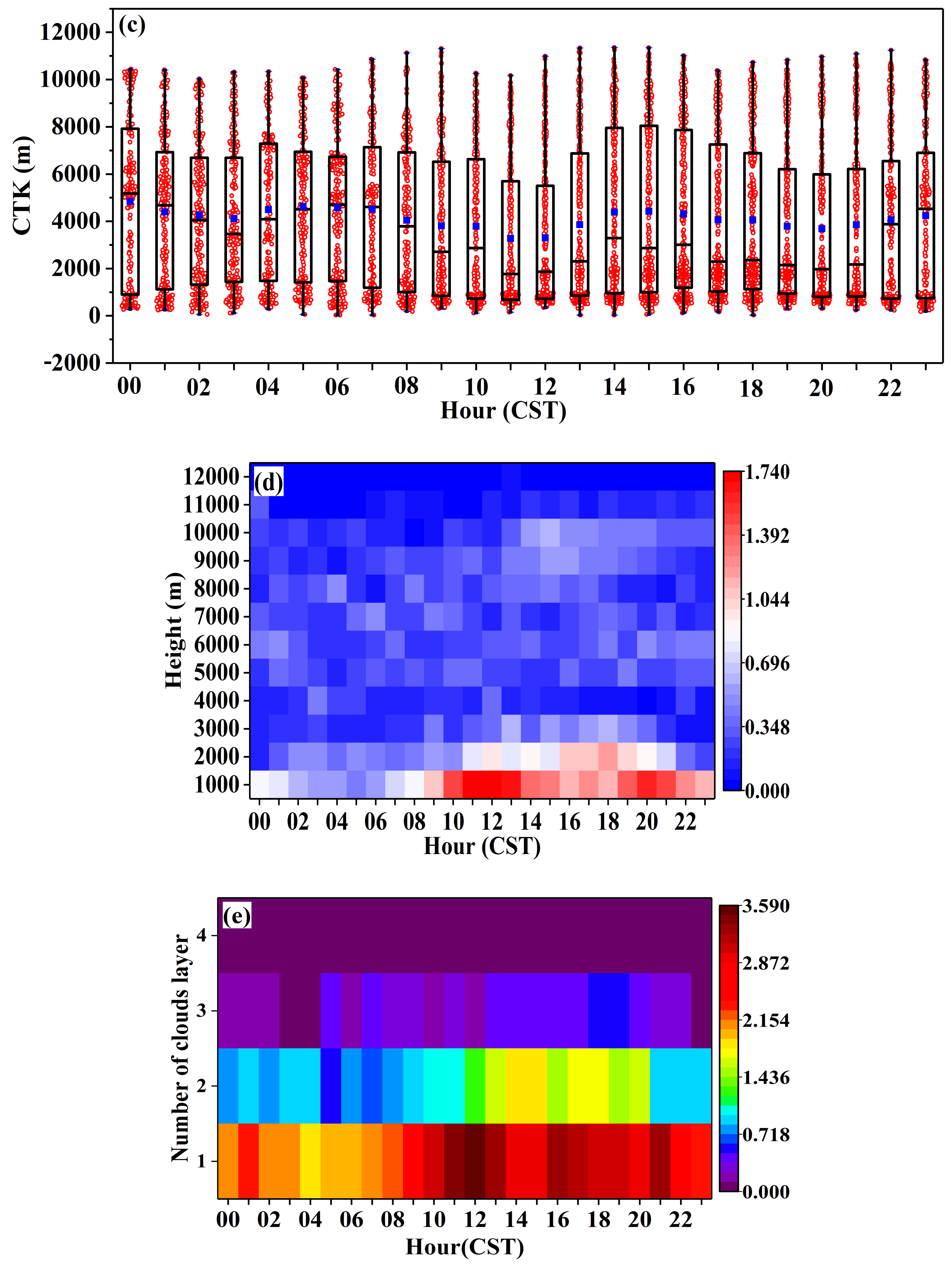
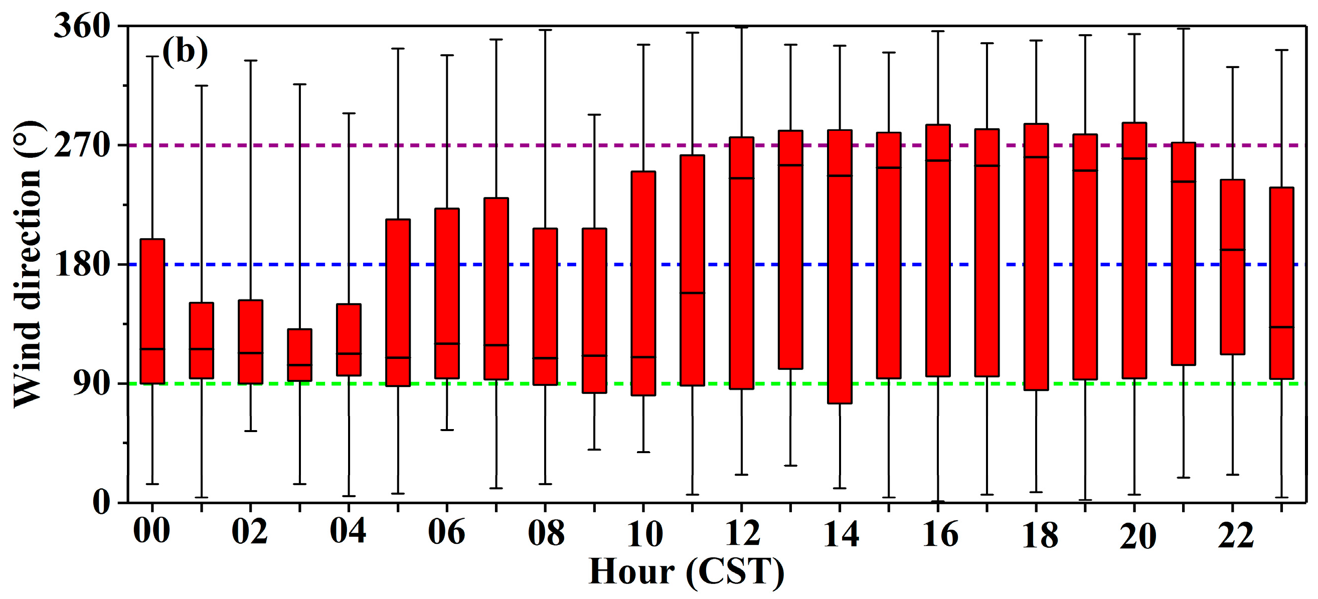
- Approximately half of CBHs, CTHs, and CTKs varied from 60 to 2075 m, 4350 to 7715 m, and 1770 to 5181 m, respectively. Diurnal variation shows a decreasing trend of CBHs from 05:00 to 19:00 CST and a rising trend of CBHs from 20:00 to 04:00 CST. The CTHs show the rising trend from 03:00 to 05:00 CST, 12:00 to 14:00 CST, and 20:00 to 01:00 CST, respectively, and 75% of the total samples of CTHs were above 5000 m from 00:00 to 09:00 CST. There was also a large number of CTHs below 3 km from 10:00 to 23:00 CST. Approximately 50% of the CTKs show the characteristics of the diurnal variation similar to the CTHs. The CTKs less than 2 km and the frequency distribution of CLNs are significantly increased from 10:00 to 23:00 CST. There are three obvious precipitation periods during the day, namely, 02:00–09:00 CST, 12:00 CST, and 17:00–21:00 CST, and the three periods produced 79.18% of the entire accumulated rain amount and 68.48% of the entire accumulated rainy minute numbers, and there were larger Rs and LWCs during the three periods. Other physical parameters also showed diurnal variation. In general, the changes were more evident during the period 12:00–21:00 CST. The diurnal variation of clouds is mainly driven by wind and temperature closely related to the topography of the study area, and the daily variation of rainfall is mainly determined by the time period of the specific rainfall process, and temperature also plays a certain role.
- The DSD is in good agreement with a normalized gamma distribution. The average value of microphysical parameters for the Nt, log10Nw, W, R, Dm, and Z of stratiform precipitation are 312 m−3, 3.86 m−3 · mm−1, 0.07 g · m−3, 0.89 mm · h−1, 0.90 mm, and 19.24 dBZ, respectively, and the values of these physical quantities for stratocumulus precipitation are slightly larger, and the shape factor μare 9.74 and 8.76, respectively, which are quite different from the fixed value in the microphysical parameterization scheme in WRF. The rain in arid Xinjiang had a relatively higher concentration of raindrops and a smaller average raindrop diameter than the rain in humid regions. The fitting equation of , , , and relationship for stratiform precipitation suitable for Xinjiang are , , , and , respectively.
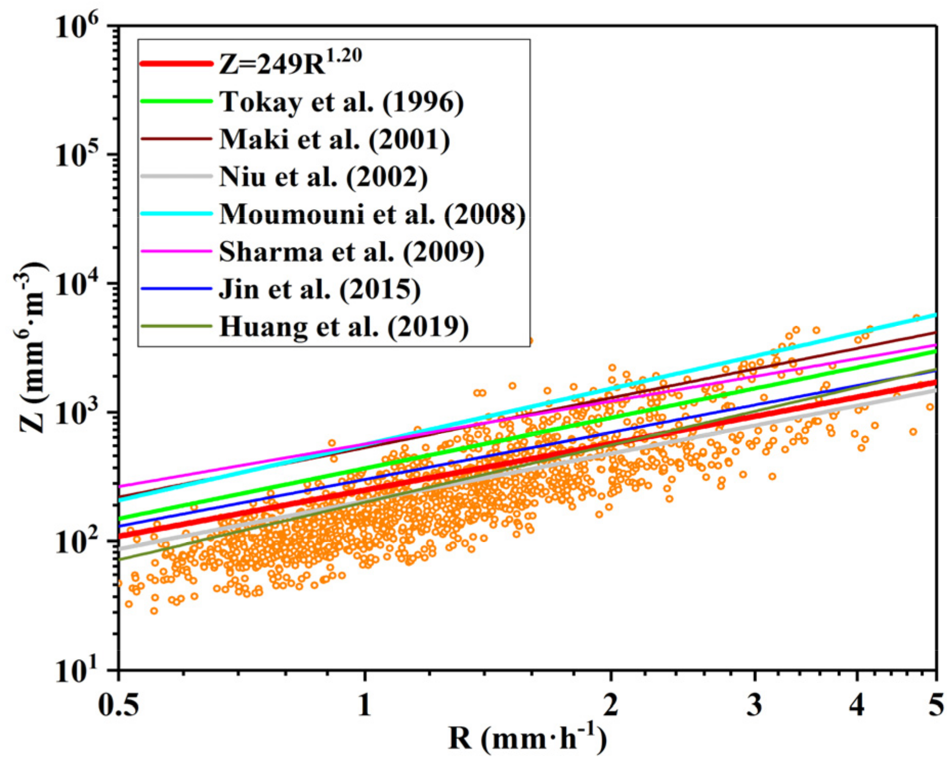
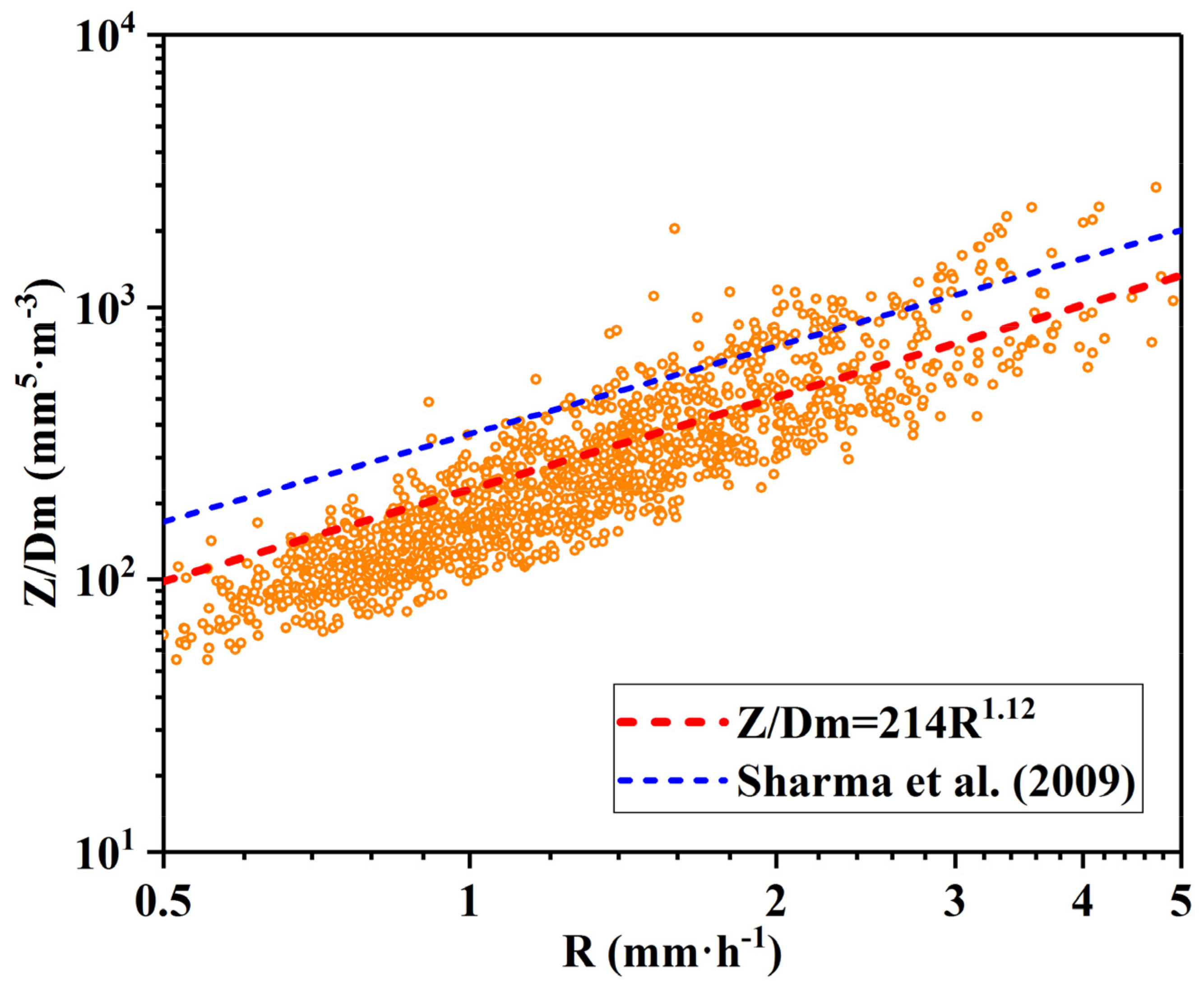
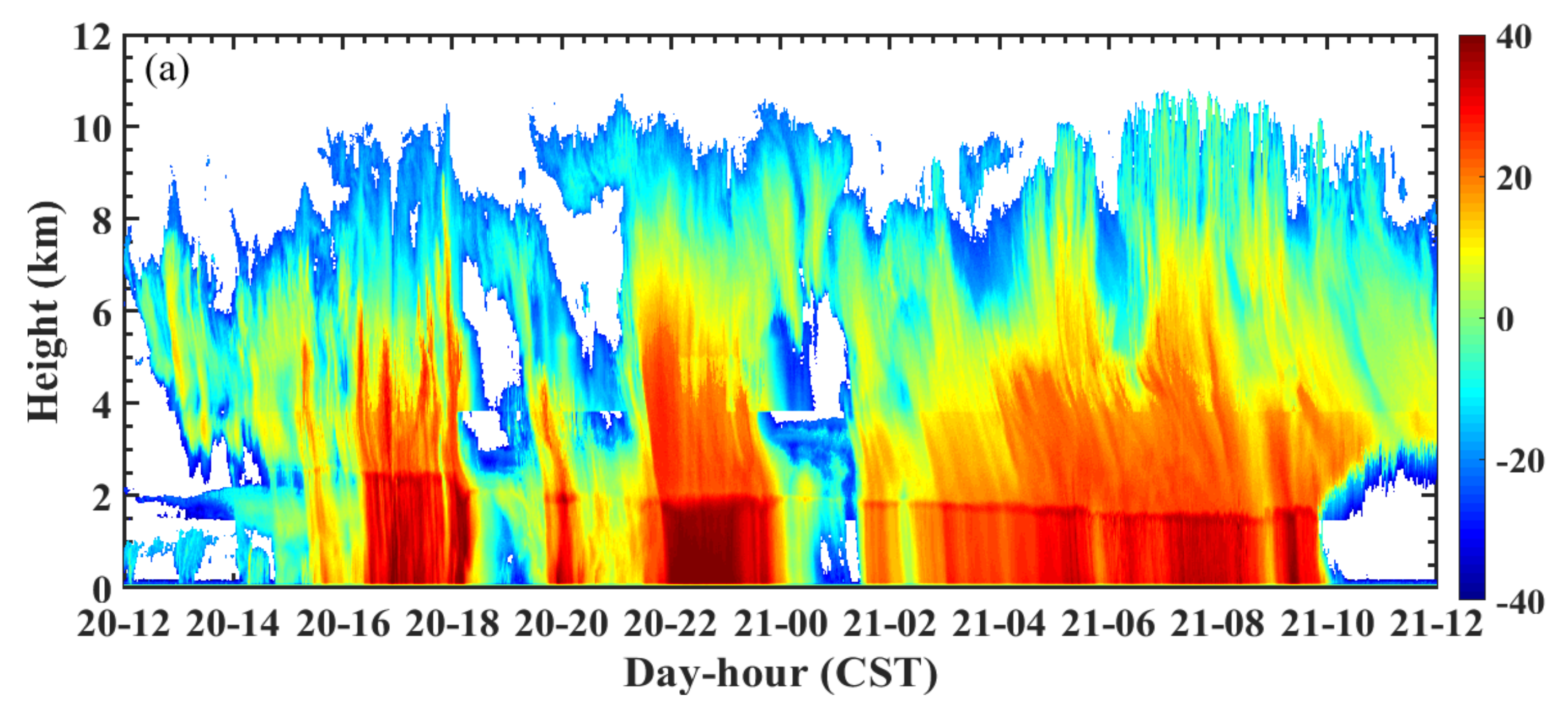
- For the arid Xinjiang, the relationship of stratiform precipitation is . The correlation coefficient of relationship is 0.78, and the RMSE of R measured by the disdrometer and R derived from the relationship is 0.99 mm · h−1. and R are used to establish a new empirical relationship for stratiform rainfall. The correlation coefficient of the relationship is 0.88, and the root mean square error of the R measured by the disdrometer and the R estimated from the relationship is 0.92 mm · h−1. Improvement is obtained in rain retrieval by using the relation relative to the conventional relation. The case study of data from 20 to 21 May 2020, also verified this conclusion.
Author Contributions
Funding
Acknowledgments
Conflicts of Interest
References
- Stephens, G.L.; Tsay, S.; Stackhouse, P.W.; Flatau, P.J. The Relevance of the Microphysical and Radiative Properties of Cirrus Clouds to Climate and Climatic Feedback. J. Atmos. Sci. 1990, 47, 1742–1753. [Google Scholar] [CrossRef]
- Heymsfield, A.J.; Platt, C.M.R. A Parameterization of the Particle Size Spectrum of Ice Clouds in Terms of the Ambient Temperature and the Ice Water Content. J. Atmos. Sci. 1984, 41, 846–855. [Google Scholar] [CrossRef]
- Ding, S.G.; Shi, G.Y.; Zhao, C.S. Analysis of variation and effect on the climate of cloud amount in China over past 20 years using ISCCP D2. Chin. Sci. Bull. 2004, 49, 1105–1111. (In Chinese) [Google Scholar]
- Zhao, C.S.; Tie, X.; Brasseur, G. Aircraft measurements of cloud droplet spectral dispersion and implications for indirect aerosol radiative forcing. Geophys. Res. Lett. 2006, 33. [Google Scholar] [CrossRef]
- Ackerman, T.P.; Stokes, G.M. The Atmospheric Radiation Measurement Program. Phys. Today 2003, 56, 38–45. [Google Scholar] [CrossRef]
- Harrison, E.F.; Minnis, P.; Barkstrom, B.R.; Ramanathan, V.; Cess, R.D.; Gibson, G.G. Seasonal variation of cloud radiative forcing derived from the earth radiation budget experiment. J. Geophys. Res. 1990, 95, 18687–18703. [Google Scholar] [CrossRef]
- Schiffer, R.A.; Rossow, W.B. The International Satellite Cloud Climatology Project (ISCCP)—The first project of the World Climate Research Programme. Bull. Am. Meteorol. Soc. 1983, 64. [Google Scholar] [CrossRef]
- Reddy, N.N.; Ratnam, M.V.; Basha, G.; Ravikiran, V. Cloud Vertical Structure over A Tropical Station Obtained Using Long-term High-resolution Radiosonde Measurements. Atmos. Chem. Phys. 2018, 18, 11709–11727. [Google Scholar] [CrossRef]
- Chen, S.S.; Kerns, B.W.; Guy, N.; Jorgensen, D.P.; Savarin, A. Aircraft Observations of Dry Air, the ITCZ, Convective Cloud Systems, and Cold Pools in MJO during DYNAMO. Bull. Am. Meteorol. Soc. 2016, 97, 405–423. [Google Scholar] [CrossRef]
- Yang, Y.J.; Lu, D.R.; Fu, Y.F.; Chen, F.J.; Wang, Y. Spectral Characteristics of Tropical Anvils Obtained by Combining TRMM Precipitation Radar with Visible and Infrared Scanner Data. Pure Appl. Geophys. 2015, 172, 1717–1733. [Google Scholar] [CrossRef]
- Parish, T.R.; Rahn, D.A.; Leon, D. Aircraft Observations of a Coastally Trapped Wind Reversal off the California Coast. Mon. Weather Rev. 2008, 136, 644–662. [Google Scholar] [CrossRef][Green Version]
- Parish, T.R.; Leon, D. Measurement of Cloud Perturbation Pressures Using an Instrumented Aircraft. J. Atmos. Ocean. Tech. 2013, 30, 215–229. [Google Scholar] [CrossRef][Green Version]
- Field, P.R.; Furtado, K. How Biased Is Aircraft Cloud Sampling? J. Atmos. Ocean. Tech. 2016, 33, 185–189. [Google Scholar] [CrossRef]
- Dong, X.; Minnis, P.; Xi, B. A climatology of midlatitude continental clouds from ARM SGP site: Part, I. Low-level cloud macrophysical, microphysical and radiative properties. J. Clim. 2005, 18, 1391–1410. [Google Scholar] [CrossRef]
- Xi, B.; Dong, X.; Minnis, P. A 10 year climatology of cloud cover and vertical distribution from both surface and GOES observations over DOE ARM SGP site. J. Geophys. Res. 2009, 115, D12. [Google Scholar] [CrossRef]
- Hou, A.Y.; Skofronick-Jackson, G.; Stocker, E.F. The Global Precipitation Measurement (GPM) Mission: Overview and U.S. Science Status. Bull. Am. Meteorol. Soc. 2014, 95, 701–722. [Google Scholar] [CrossRef]
- Kollias, P.; Clothiaux, E.E.; Miller, M.M. Millimeter-wavelength radars: New frontier in atmospheric cloud and precipitation research. Bull. Am. Meteorol. Soc. 2007, 88, 1608–1624. [Google Scholar] [CrossRef]
- Moran, K.P.; Martner, B.E.; Post, M.J.; Kropfli, R.A.; Widener, K.B. An Unattended Cloud-Profiling Radar for Use in Climate Research. Bull. Amer. Meteorol. Soc. 1998, 79, 443–455. [Google Scholar] [CrossRef]
- Kollias, P.; Jasmine, R.; Edward, L.; Wanda, S. Cloud radar Doppler spectra in drizzling stratiform clouds: 1. Forward modeling and remote sensing applications. J. Geophys. Res. 2011, 116. [Google Scholar] [CrossRef]
- Liu, L.; Ruan, Z.; Zheng, J.; Gao, W. Comparing and Merging Observation Data from Ka-band Cloud Radar, C-band Frequency-modulated Continuous Wave Radar and Ceilometer Systems. Remote Sens. 2017, 9, 1282. [Google Scholar] [CrossRef]
- Zheng, J.; Liu, L.; Chen, H.; Gou, Y.; Che, Y.; Xu, H.; Li, Q. Characteristics of Warm Clouds and Precipitation in South China during the Pre-Flood Season Using Datasets from a Cloud Radar, a Ceilometer, and a Disdrometer. Remote Sens. 2019, 11, 3045. [Google Scholar] [CrossRef]
- Marshall, J.S.; Palmer, W.M.K. The Distribution of Raindrops with Size. J. Atmos. Sci. 1948, 5, 165–166. [Google Scholar] [CrossRef]
- Geoffroy, O.; Siebesma, A.P.; Burnet, F. Characteristics of the raindrop distributions in RICO shallow cumulus. Atmos. Chem. Phys. 2014, 14, 10897–10909. [Google Scholar] [CrossRef]
- Krishna, U.V.M.; Reddy, K.K.; Seela, B.K. Raindrop size distribution of easterly and westerly monsoon precipitation observed over Palau islands in the western Pacific Ocean. Atmos. Res. 2016, 174, 41–51. [Google Scholar] [CrossRef]
- Hazenberg, P.; Yu, N.; Boudevillain, B.; Delrieu, G.; Uijlenhoet, R. Scaling of raindrop size distributions and classification of radar reflectivity–rain rate relations in intense Mediterranean precipitation. J. Hydrol. 2011, 402, 179–192. [Google Scholar] [CrossRef]
- Tokay, A.; Short, D.A. Evidence from tropical raindrop spectra of the origin of rain from stratiform versus convective clouds. J. Appl. Meteor. 1996, 35, 355–371. [Google Scholar] [CrossRef]
- Bringi, V.N.; Chandrasekar, V.; Hubbert, J.; Gorgucci, E.; Randeu, W.L.; Schoenhuber, M. Raindrop size distribution in different climatic regimes from disdrometer and dualpolarized radar analysis. J. Atmos. Sci. 2003, 60, 354–365. [Google Scholar] [CrossRef]
- Ulbrich, C.W.; Atlas, D. Microphysics of raindrop size spectra: Tropical continental and maritime storms. J. Appl. Meteor. Climatol. 2007, 46, 1777–1791. [Google Scholar] [CrossRef]
- Joss, J.; Waldvogel, A. Ein Spektrograph für Niederschlagstropfen mit automatischer Auswertung. Pure Appl. Geophys. 1967, 68, 240–246. [Google Scholar] [CrossRef]
- Löffler-Mang, M.; Joss, J. An Optical Disdrometer for Measuring Size and Velocity of Hydrometeors. J. Atmos. Ocean. Technol. 2000, 17, 130–139. [Google Scholar] [CrossRef]
- Schönhuber, M.; Lammer, G.; Randeu, W.L. One decade of imaging precipitation measurement by 2D-video-distrometer. Adv. Geosci. 2007, 10, 85–90. [Google Scholar] [CrossRef]
- Islam, T.; Rico-Ramirez, M.A.; Thurai, M. Characteristics of raindrop spectra as normalized gamma distribution from a Joss-Waldvogel disdrometer. Atmos. Res. 2012, 108, 57–73. [Google Scholar] [CrossRef]
- Chen, B.J.; Yang, J.; Pu, J.P. Statistical characteristics of raindrop size distribution in the Meiyu season observed in eastern China. J. Meteor. Soc. Jpn. 2013, 91, 215–227. [Google Scholar] [CrossRef]
- Marzano, F.S.; Cimini, D.; Montopoli, M. Investigating precipitation microphysics using ground-based microwave remote sensors and disdrometer data. Atmos. Res. 2010, 97, 583–600. [Google Scholar] [CrossRef]
- Chen, B.J.; Hu, Z.Q.; Liu, L.P.; Zhang, G.F. Raindrop size distribution measurements at 4,500 m on the Tibetan Plateau during TIPEX-III. J. Geophys. Res. 2017, 122, 11092–11106. [Google Scholar] [CrossRef]
- Comstock, K.K.; Wood, R.; Yuter, S.E.; Bretherton, C.S. Reflectivity and rain rate in and below drizzling stratocumulus. Q. J. R. Meteorol. Soc. 2004, 130, 2891–2918. [Google Scholar] [CrossRef]
- Tokay, A.; Kruger, A.; Krajewski, W.F.; Kucera, P.A.; Filho, A.J.P. Measurements of drop size distribution in the southwestern Amazon basin. J. Geophys. Res. 2002, 107. [Google Scholar] [CrossRef]
- Atlas, D.; Ulbrich, C.W.; MarksJr, F.D.; Amitai, E.; Williams, C.R. Systematic variation of drop size and radar-rainfall relations. J. Geophys. Res. 1999, 104, 6155–6169. [Google Scholar] [CrossRef]
- Maki, M.; Keenan, T.D.; Sasaki, Y.; Nakamura, K. Characteristics of the raindrop size distribution in tropical continental squall lines observed in Darwin, Australia. J. Appl. Meteor. 2001, 40, 1393–1412. [Google Scholar] [CrossRef]
- Reddy, K.K.; Kozu, T. Measurement of rain drop size distribution over Gadanki during south–west and north–east monsoon. Indian J. Radio Space Phys. 2003, 32, 286–295. [Google Scholar]
- Sharma, S.; Konwar, M.; Sarma, D.K.; Kalapureddy, M.C.R.; Jain, A.R. Characteristics of Rain Integral Parameters during Tropical Convective, Transition, and Stratiform Rain at Gadanki and Its Application in Rain Retrieval. J. Appl. Meteor. Climatol. 2009, 48, 1245–1266. [Google Scholar] [CrossRef]
- Wu, Y.; Liu, L. Statistical characteristics of raindrop size distribution in the Tibetan Plateau and southern China. Adv. Atmos. Sci. 2017, 34, 727–736. [Google Scholar] [CrossRef]
- Wen, L.; Zhao, K.; Wang, M.Y.; Zhang, G.F. Seasonal variations of observed raindrop size distribution in East China. Adv. Atmos. Sci. 2019, 36, 346–362. [Google Scholar] [CrossRef]
- Yang, Q.Q.; Dai, Q.; Han, D.W.; Chen, Y.H.; Zhang, S.L. Sensitivity analysis of raindrop size distribution parameterizations in WRF rainfall simulation. Atmos. Res. 2019, 228, 1–13. [Google Scholar] [CrossRef]
- Brown, B.R.; Bell, M.M.; Frambach, A.J. Validation of simulated hurricane drop size distributions using polarimetric radar. Geophys. Res. Lett. 2016, 43, 910–917. [Google Scholar] [CrossRef]
- Khain, A.; Lynn, B.; Shpund, J. High resolution WRF simulations of Hurricane Irene: Sensitivity to aerosols and choice of microphysical schemes. Atmos. Res. 2016, 167, 129–145. [Google Scholar] [CrossRef]
- Kala, J.; Andrys, J.; Lyons, T.J.; Foster, I.J.; Evans, B.J. Sensitivity of WRF to driving data and physics options on a seasonal time-scale for the southwest of Western Australia. Clim. Dyn. 2015, 44, 633–659. [Google Scholar] [CrossRef]
- Gilmore, M.S.; Straka, J.M.; Rasmussen, E.N. Precipitation uncertainty due to variations in precipitation particle parameters within a simple microphysics scheme. Mon. Weather Rev. 2004, 132, 2610–2627. [Google Scholar] [CrossRef]
- Chen, F.H.; Yu, Z.C.; Yang, M.L. Holocene moisture evolution in arid central Asia and its out-of-phase relationship with Asian monsoon history. Quat. Sci. Rev. 2008, 27, 351–364. [Google Scholar] [CrossRef]
- Huang, W.; Chang, S.Q.; Xie, C.L. Moisture sources of extreme summer precipitation events in North Xinjiang and their relationship with atmospheric circulation. Adv. Clim. Chang. Res. 2017, 8, 12–17. [Google Scholar] [CrossRef]
- Huang, W.; Feng, S.; Chen, J. Physical Mechanisms of Summer Precipitation Variations in the Tarim Basin in Northwestern China. J. Clim. 2015, 28, 3579–3591. [Google Scholar] [CrossRef]
- Zeng, Y.; Yang, L.M. Triggering Mechanism of an Extreme Rainstorm Process near the Tianshan Mountains in Xinjiang, an Arid Region in China, Based on a Numerical Simulation. Adv. Meteorol. 2020, 2020. [Google Scholar] [CrossRef]
- Zeng, Y.; Zhou, Y.S.; Yang, L.M. A preliminary analysis of the formation mechanism for a heavy rainstorm in western Xinjiang by numerical simulation. Chin. J. Atmos. Sci. 2019, 43, 372–388. (In Chinese) [Google Scholar]
- Lim, K.-S.S.; Hong, S.-Y. Development of an effective double-moment cloud microphysics scheme with prognostic cloud condensation nuclei (CCN) for weather and climate models. Mon. Weather Rev. 2010, 138, 1587–1612. [Google Scholar] [CrossRef]
- Thompson, G.; Eidhammer, T. A study of aerosol impacts on clouds and precipitation development in a large winter cyclone. J. Atmos. Sci. 2014, 71, 3636–3658. [Google Scholar] [CrossRef]
- Zeng, Y.; Yang, L.M. Comparative analysis on mesoscale characteristics of two severe short-time precipitation events in the west of southern Xinjiang. Torrential Disasters 2017, 36, 410–421. (In Chinese) [Google Scholar]
- Liu, L.; Zheng, J. Algorithms for Doppler Spectral Density Data Quality Control and Merging for the Ka-Band Solid-State Transmitter Cloud Radar. Remote Sens. 2019, 11, 209. [Google Scholar] [CrossRef]
- Battaglia, A.; Rustemeier, E.; Tokay, A. PARSIVEL snow observations: A critical assessment. J. Atmos. Oceanic Technol. 2010, 27, 333–344. [Google Scholar] [CrossRef]
- Testud, J.S.; Oury, S.; Black, R.A.; Amayenc, P.; Dou, X. The concept of “normalized” distribution to describe raindrop spectra: A tool for cloud physics and cloud remote sensing. J. Appl. Meteor. 2001, 40, 1118–1140. [Google Scholar] [CrossRef]
- Ulbrich, C.W. Natural Variations in the Analytical Form of the Raindrop Size Distribution. J. Clim. Appl. Meteorol. 1983, 22, 1764–1775. [Google Scholar] [CrossRef]
- Willis, P.T. Functional fits to some observed drop size distributions and parameterization of rain. J. Atmos. Sci. 1984, 41, 1648–1661. [Google Scholar] [CrossRef]
- Illingworth, A.J.; Blackman, T.M. The need to represent raindrop size spectra as normalized gamma distributions for the interpretation of polarization radar observations. J. Appl. Meteor. 2002, 41, 286–297. [Google Scholar] [CrossRef]
- Torres, D.S.; Porrà, J.M.; Creutin, J.D. A general formulation for raindrop size distribution. J. Appl. Meteor. 1994, 33, 1494–1502. [Google Scholar] [CrossRef]
- Kozu, T.; Nakamura, K. Rainfall parameter estimation from dual-radar measurements combining reflectivity profile and path-integrated attenuation. J. Atmos. Ocean. Technol. 1991, 8, 259–271. [Google Scholar] [CrossRef]
- Lam, H.Y.; Din, J.; Jong, S.L. Statistical and physical descriptions of raindrop size distributions in equatorial Malaysia from disdrometer observations. Adv. Meteorol. 2015, 2015. [Google Scholar] [CrossRef]
- Li, H.; Yin, Y.; Shan, Y.P. Statistical characteristics of raindrop size distribution for stratiform and convective precipitation at different altitudes in Mt. Huangshan. Chin. J. Atmos. Sci. 2018, 42, 268–280. (In Chinese) [Google Scholar]
- Chen, C.; Yin, Y.; Chen, B.J. Raindrop Size Distribution at Different Altitudes in Mt. Huang. Trans. Atmos. Sci. 2015, 38, 388–395. [Google Scholar]
- Villalobos-Puma, E.; Martinez-Castro, D.; Flores-Rojas, J.L.; Saavedra-Huanca, M.; Silva-Vidal, Y. Diurnal Cycle of Raindrops Size Distribution in a Valley of the Peruvian Central Andes. Atmosphere 2020, 11, 38. [Google Scholar] [CrossRef]
- Jin, Q.; Yuan, Y.; Liu, H.J.; Shi, C.E.; Li, J.B. Analysis of microphysical characteristics of the raindrop spectrum over the area between the Yangtze River and the Huaihe River during summer. Acta Meteorol. Sin. 2015, 73, 778–788. (In Chinese) [Google Scholar]
- Rosenfeld, D.; Ulbrich, C.W. Cloud Microphysical Properties, Processes, and Rainfall Estimation Opportunities. Meteorol. Monogr. 2003, 30, 237–258. [Google Scholar] [CrossRef]
- Niu, S.J.; An, X.L.; Sang, J.R. Observational Research on Physical Feature of Summer Rain Dropsize Distribution under Synoptic Systems in Ningxia. Plateau Meteor. 2002, 21, 37–44. (In Chinese) [Google Scholar]
- Moumouni, S.; Gosset, M.; Houngninou, E. Main features of rain drop size distributions observed in Benin, West Africa, with optical disdrometers. Geophys. Res. Lett. 2008, 35, 23. [Google Scholar] [CrossRef]
- Huang, X.Y.; Yin, J.N.; Ma, L. Comprehensive statistical analysis of rain drop size distribution parameters and their application to weather radar measurement in Nanjing. Chin. J. Atmos. Sci. 2019, 43, 691–704. (In Chinese) [Google Scholar]
- Zhang, A.S.; Hu, J.J.; Chen, S.; Hu, D.M.; Liang, Z.Q.; Huang, C.Y. Statistical Characteristics of Raindrop Size Distribution in the Monsoon Season Observed in Southern China. Remote Sens. 2019, 11, 432. [Google Scholar] [CrossRef]


| Rain Type | Nt (m−3) | log10Nw (m−3 · mm−1) | W (g · m−3) | R (mm · h−1) | Dm (mm) | Z (dBZ) | μ |
|---|---|---|---|---|---|---|---|
| Stratiform | 312 | 3.86 | 0.07 | 0.89 | 0.90 | 19.24 | 9.74 |
| Stratocumulus | 351 | 3.89 | 0.08 | 0.90 | 0.94 | 20.85 | 8.76 |
| Relation | log10Nt–R | Dm–R | log10Nw–R | log10Nw–log10Nt | Z–R | Z/Dm–R |
|---|---|---|---|---|---|---|
| Correlation coefficient | 0.65 | 0.62 | 0.22 | 0.85 | 0.78 | 0.88 |
| Number of Rain Event | Start and End Time (Month/Day/Hour:Minute) | Accumulated Rain Amount (mm) | Average Rainfall Intensity (mm · h−1) |
|---|---|---|---|
| 1 | 3/6/11:55–3/6/12:52 | 0.80 | 0.83 |
| 2 | 3/6/16:48–3/6/18:46 | 0.45 | 0.23 |
| 3 | 3/20/05:40–3/20/16:19 | 7.29 | 1.07 |
| 4 | 3/22/15:46–3/22/19:09 | 1.53 | 0.45 |
| 5 | 3/24/02:02–3/24/02:35 | 0.22 | 0.39 |
| 6 | 3/29/03:51–3/29/08:42 | 2.70 | 0.89 |
| 7 | 4/9/18:41–4/9/19:43 | 0.58 | 0.56 |
| 8 | 4/14/08:45–4/14/09:49 | 0.87 | 0.80 |
| 9 | 4/15/11:13–4/15/12:30 | 0.36 | 0.28 |
| 10 | 4/15/18:03–4/16/05:06 | 8.72 | 0.97 |
| 11 | 4/18/02:19–4/18/09:10 | 0.19 | 0.21 |
| 12 | 4/30/18:23–4/30/23:57 | 8.16 | 1.46 |
| 13 | 5/3/23:45–5/4/10:52 | 12.12 | 1.15 |
| 14 | 5/15/08:32–5/15/10:27 | 1.15 | 0.60 |
| 15 | 5/20/16:25–5/20/18:18 | 2.00 | 1.05 |
| 16 | 5/20/21:32–5/21/00:00 | 3.80 | 1.53 |
| 17 | 5/21/03:01–5/21/09:58 | 3.35 | 0.55 |
Publisher’s Note: MDPI stays neutral with regard to jurisdictional claims in published maps and institutional affiliations. |
© 2020 by the authors. Licensee MDPI, Basel, Switzerland. This article is an open access article distributed under the terms and conditions of the Creative Commons Attribution (CC BY) license (http://creativecommons.org/licenses/by/4.0/).
Share and Cite
Zeng, Y.; Yang, L.; Zhang, Z.; Tong, Z.; Li, J.; Liu, F.; Zhang, J.; Jiang, Y. Characteristics of Clouds and Raindrop Size Distribution in Xinjiang, Using Cloud Radar Datasets and a Disdrometer. Atmosphere 2020, 11, 1382. https://doi.org/10.3390/atmos11121382
Zeng Y, Yang L, Zhang Z, Tong Z, Li J, Liu F, Zhang J, Jiang Y. Characteristics of Clouds and Raindrop Size Distribution in Xinjiang, Using Cloud Radar Datasets and a Disdrometer. Atmosphere. 2020; 11(12):1382. https://doi.org/10.3390/atmos11121382
Chicago/Turabian StyleZeng, Yong, Lianmei Yang, Zuyi Zhang, Zepeng Tong, Jiangang Li, Fan Liu, Jinru Zhang, and Yufei Jiang. 2020. "Characteristics of Clouds and Raindrop Size Distribution in Xinjiang, Using Cloud Radar Datasets and a Disdrometer" Atmosphere 11, no. 12: 1382. https://doi.org/10.3390/atmos11121382
APA StyleZeng, Y., Yang, L., Zhang, Z., Tong, Z., Li, J., Liu, F., Zhang, J., & Jiang, Y. (2020). Characteristics of Clouds and Raindrop Size Distribution in Xinjiang, Using Cloud Radar Datasets and a Disdrometer. Atmosphere, 11(12), 1382. https://doi.org/10.3390/atmos11121382