Article

Detection of Airborne Biological Particles in Indoor Air Using a Real-Time Advanced Morphological Parameter UV-LIF Spectrometer and Gradient Boosting Ensemble Decision Tree Classifiers

1
Department of Earth and Environmental Sciences, The University of Manchester, Manchester M13 9PL, UK
2
Defence Science and Technology Laboratory, Porton Down, Salisbury SP4 0JQ, UK
3
Particle Instruments & Diagnostics Research Group, University of Hertfordshire, Hatfield, Hertfordshire AL10 9AB, UK
*
Author to whom correspondence should be addressed.
Atmosphere 2020, 11(10), 1039; https://doi.org/10.3390/atmos11101039
Submission received: 29 July 2020 / Revised: 17 September 2020 / Accepted: 23 September 2020 / Published: 29 September 2020

Abstract

:
We present results from a study evaluating the utility of supervised machine learning to classify single particle ultraviolet laser-induced fluorescence (UV-LIF) signatures to investigate airborne primary biological aerosol particle (PBAP) concentrations in a busy, multifunctional building using a Multiparameter Bioaerosol Spectrometer. First we introduce and demonstrate a gradient boosting ensemble decision tree algorithm’s ability to accurately classify laboratory generated PBAP samples into broad taxonomic classes with a high level of accuracy. We then develop a framework to appraise the classification accuracy and performance using the Hellinger distance metric to compare product parameter probability density function similarity; this framework showed that key training classes were sufficiently different in terms of particle fluorescence and morphology to facilitate classification. We also demonstrate the utility of including advanced morphological parameters to minimise inter-class conflation and improve classification confidence, where relying on the fluorescent spectra alone would likely result in misattribution. Finally, we apply these methods to ambient data collected within a large multi-functional building where ambient bacterial- and fungal-like classes were identified to display trends corresponding to human activity; fungal-like classes displayed a consistent diurnal trend with a maximum at midday and hourly peaks correlating to movements within the building; bacteria-like aerosol displayed complex, episodic events during opening hours. All PBAP classes fell to low baseline concentrations when the building was unoccupied overnight and at weekends.

1. Introduction

Primary Biological Aerosol Particles (PBAP) are a diverse and complex classification of aerosol which are ubiquitous in the atmosphere and built up environment, accounting for >25% of global organic aerosol emissions and >10% of global continental supermicron number concentrations [1,2]. They span a large range of particle sizes from 10′s of nanometers (viruses) to up to 100 µm (pollen) and display highly complex species dependent morphologies. The atmospheric science community has recently taken a renewed interest in certain PBAP classes owing to their potential to nucleate ice particles and thus take part in global hydrological processes, the emission of which may display sensitivity to a changing climate [3,4,5,6]. In additional to their potential climatological significance PBAP also impact agricultural, animal and human health via direct and indirect pathogenic processes causing personal and economic harm [7,8,9].
Indoor air quality can be significantly impacted by the presence of biological aerosol. So called sick building syndrome is a condition where occupants experience adverse health effects (e.g., headaches, shortness of breath, tiredness and throbbing sensations) strongly related to time spent indoors [10,11]. Societal and life style changes dictate that people spend an increasing and substantial portion of their time indoors, increasing exposure to potential allergenic and pathogenic PBAP [12]. The UK has one of the highest prevalence of diagnosed asthma affecting around 10% of the adult population [13,14]; currently, over 150 million people in the EU suffer from chronic allergenic diseases and by 2025 it is thought that half of the population will be affected with impairment of individual’s quality of life and loss of productivity. As such, there is an increasing need to understand how indoor air quality impacts human health and quality of life.
Indoor fungal pollution poses a serious threat to public health [15], where many fungi reported in building mycology surveys are known human allergens. Fungi have been demonstrated to grow on a wide range of natural and synthetic materials common in the indoor environment, especially if exposed to moisture. Inorganic materials are readily colonised via dust absorption and present ideal growth environments for allergenic Aspergillius species; species belonging to Aspergillius, Cladosporium and Penicillium are also especially prevalent in wood and processed wood products used as building materials [16,17]. Khan and Karuppayil (2012) [15] present a synthesis of global studies investigating indoor fungal species in different environments. While they report a wide range in diversity in the surveyed indoor mycology studies, a few notable species such as Aspergillius, Cladosporium and Penicillium were commonly identified. Indoor bacteria such as Legionella may proliferate in air conditioning systems and water pipes which when aerosolised may cause Legionnaire’s Disease, where stagnant showers are thought to be a significant exposure risk [18]. Handorean et al. [19] demonstrated that soiled textiles are a significant source of bacterial aerosol in indoor healthcare environments, where routine handling and storage may provide an aerosolization mechanism. Bhangar et al. [20] related observed indoor PBAP concentrations to the vigour of human activity, where they suggested that the agitation of clothing when moving may be a significant source of microbial aerosol emission.

1.1. PBAP Detection Methods

Detecting and quantifying PBAP poses a significant technical challenge with no one method providing both high temporal resolution and taxonomic specificity to date [21]. Many traditional methods rely on collecting microorganisms on a substrate for offline analysis, e.g., by visual identification under a microscope or by targeted next generation rRNA gene sequencing. While these methods can provide excellent detailed taxonomic information they offer low time resolution due to the necessity for long sampling periods to acquire sufficient bio-material for analysis; this may smear short lived emission events and obfuscate identification of underlying propagation and dispersion mechanisms.
In recent times, ultraviolet light-induced fluorescence (UV-LIF) bioaerosol spectrometers have been developed to detect PBAP in real time. Many of these instruments collect data on a particle by particle basis and thus offer excellent time resolution, limited only by the requirement of adequate sampling statistics (5 min integrations are typical). A historic limitation of UV-LIF methods is that older spectrometers do not offer enough spectral resolution or morphological detail to unambiguously classify particles (e.g., Wideband Integrated Bioaerosol Spectrometer, WIBS and the UV-APS) due to the conflation of PBAP classes. More sophisticated UV-LIF spectrometers are now becoming available which offer much greater spectral resolution and particle shape information which should significantly improve PBAP classification capability [21,22,23,24,25]. While real time UV-LIF spectrometers may not offer the specificity of offline methods, their capacity for high time resolution detection makes them ideally suited for the investigation of rapid and dynamic changes in the indoor environment and as such provide critical complementary information on real-time dispersion.

1.2. UV-LIF Classification Methods

Early UV-LIF spectrometers made a simple distinction between presumed biological and non-biological aerosol on the basis of fluorescent intensity exceeding a given threshold value (e.g., UV-APS [26]). WIBS three channel spectrometers expanded this to tryptophan-like and NADH-like fluorescence based on the dominant fluorescent channel [27]. These primitive methods allowed for the identification of illuminating trends but fall someway short of unambiguous classification.
Given the difficulty of manually analysing very large multiple parameter databases, more recent classification schemes have employed machine learning techniques to interpret data. Hierarchical agglomerative clustering (HAC) has been shown to provide useful data products when interpreting WIBS data, however, the products do not provide unambiguous classification and some level of subjective interpretation is required. Performance is also highly sensitive to data pre-processing and the choice of clustering linkage [22,28,29,30]. Additionally, HAC post-processing time cost scales with dataset size, resulting in a significant time penalty when processing large datasets.
Supervised methods seek to explicitly classify fluorescent particles into broad classes or species based on laboratory generated training datasets. The overall performance of any supervised method will therefore be constrained by the applicability of the data used to train the predictive model. Ruske et al. [22] investigated the use of several supervised and unsupervised methods to classify ambient PBAP using laboratory generated data. Generally they found that supervised methods significantly outperformed unsupervised methods, with gradient boosting ensemble decision trees (GBA) demonstrating near 100% classification accuracy at species level. The authors also noted that GBA offers a much quicker alternative to HAC once the model has been trained. As such, GBA represents the current recommended supervised learning technique for UV-LIF classification and we investigate the use of this method to interrogate and classify indoor PBAP using a broad selection of appropriate laboratory generated training data.

1.3. Aims and Objectives

The work presented in this study has the following core objectives:
  • To assess the efficiency and effectiveness of gradient boosting ensemble decision trees to accurately classify UV-LIF data into broad PBAP classes.
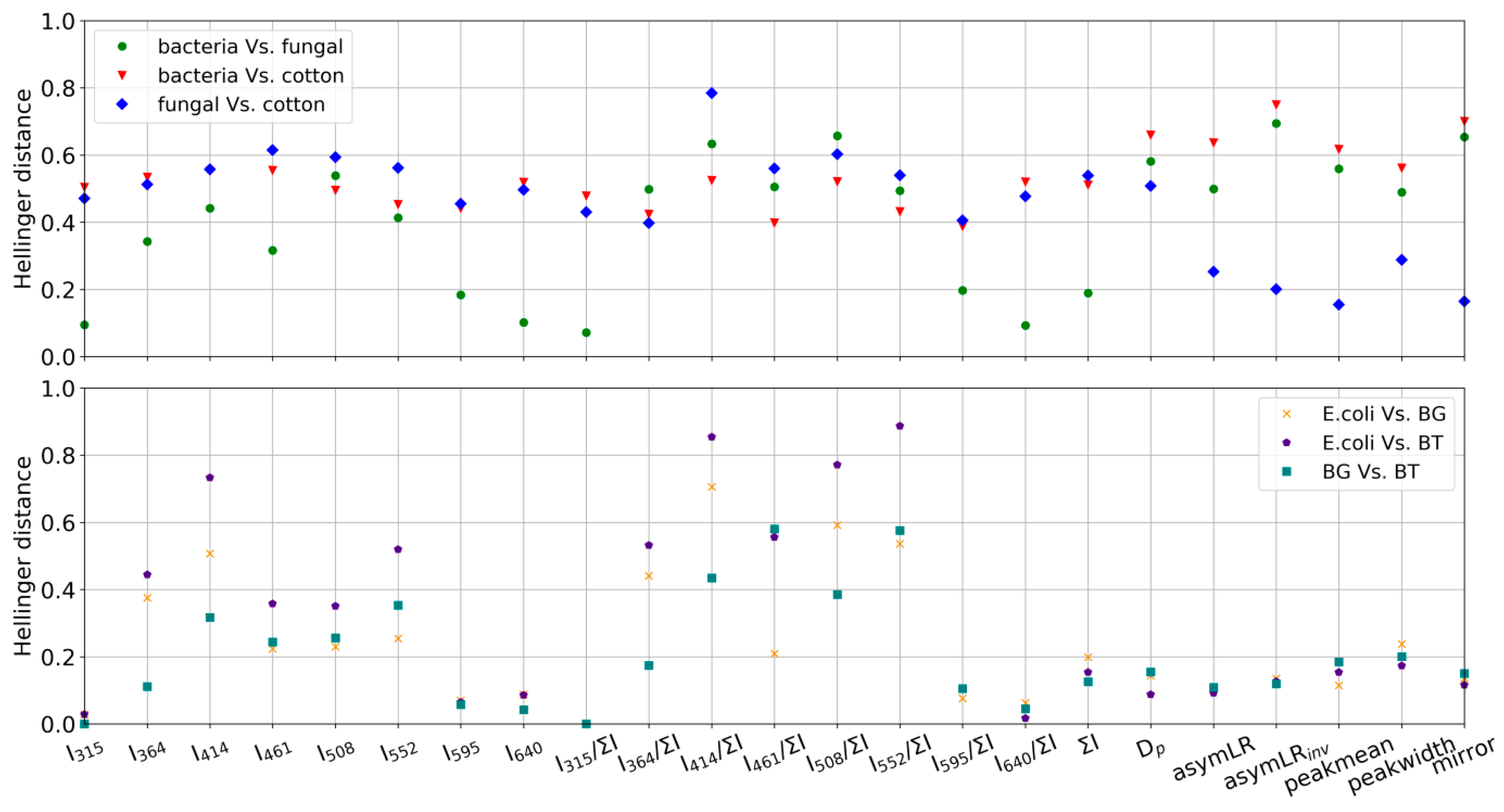
  • To develop a framework for the UV-LIF machine learning community to assess how training data may be conflated independently of the choice of classification model and to also appraise the applicability of a training dataset to generate a classification model to represent a given ambient dataset. This is achieved using the Hellinger distance metric to quantify the similarity of parameter probability distributions between training data and model outputs for each class.
  • To demonstrate real-world use of the above to quantify airborne concentrations of broad PBAP classes in a busy, multi-functional indoor environment.

2. Methods

2.1. The Multiparameter Bioaerosol Spectrometer

The Multiparameter Bioaerosol Spectrometer (MBS) is an Ultraviolet-light induced fluorescence spectrometer developed by the University of Hertfordshire, and is the next evolutionary step of such spectrometers from the WIBS which have been utilized in many real time PBAP detection experiments [31,32,33,34,35,36]. A full description of the MBS instrument is provided in Ruske et al. [22] and a brief description is now given. Similar in principle of operation and design to the WIBS, the MBS features enhanced spectral resolution boasting autofluorescent detection over 8 bands between 315–640 nm. The signal is detected via a multichannel photodetector where a grating spectrometer is used to split the incident fluorescent signal. A single optically filtered xenon flash lamp provides excitation at a wavelength of 280 nm. The resulting high resolution excitation/emission bands provide significantly reduced conflation between key biofluorophores compared to the WIBS independent broad band detectors, greatly enhancing PBAP discriminative capability [22].
Air is drawn into the MBS via an inlet featuring a removable oversized particle trap at a total flow rate of approximately 1.2 L min−1; the majority of this flow is split and filtered to provide a sheath flow. This sheath flow constrains the target aerosol into a well-defined sample flow (approximately 0.2 L min−1) to minimise contamination of the optics; it also serves to provide a single file of collimated aerosol for the detection system. Aerosol in the sensing region are first detected and sized using a 635 nm low power laser (12 mW) over a range of 0.5 to 20 µm in diameter; particles greater than a threshold size trigger a second high power 637 nm laser (250 mW) which illuminates the particle with sufficient intensity to characterise the particles morphology via a dual CMOS (complementary metal-oxide-semiconductor) image sensor array which will be described in detail later in this manuscript. The xenon flashlamp is triggered 10 µs after a critical detection event, and any resultant emission is focused onto the detection optics via two hemispherical mirrors and recorded along with all other parameters. Instrument dead time due to the xenon flashlamp recharging in between strobes limits acquisition to approximately 125 particles s−1. In practice, the instrument rarely strobes at such a high rate when sampling ambient air given its fairly coarse detection range.
The dual 512 pixel CMOS arrays collect scatted light from the particle and provide two linear sectional profiles through the 2D profile of the particle’s spatial light scattering pattern, similar in principle to the small ice detector cloud spectrometer [37]. Rather than interrogate the whole CMOS array data in post-processing, several useful parameters are calculated from the distributions at acquisition which are now described below. A schematic diagram depicting the parameters is also provided in Figure 1.
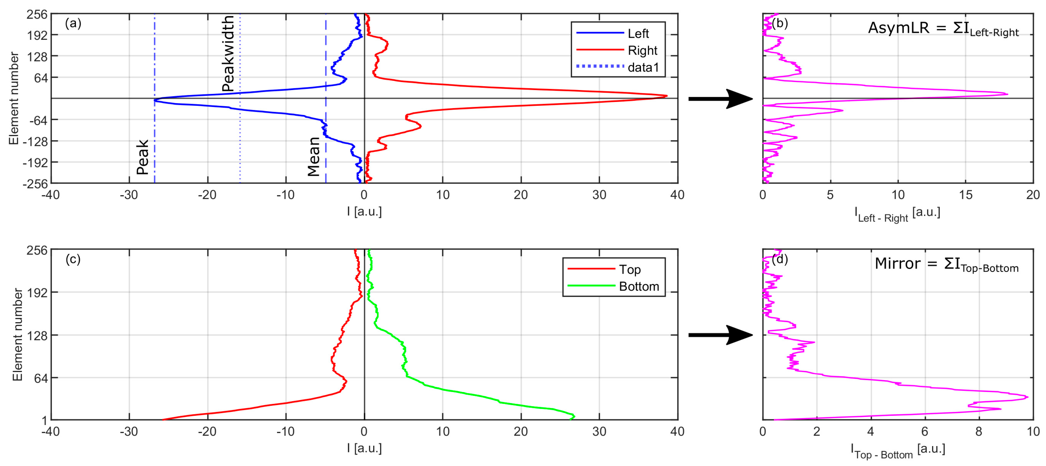
  • Peakwidth: An estimate of the mean width of the array peak, defined as the mid-point between the mean and peak values.
  • Peakmean: The ratio of the peak to mean parameters. This is a simple method of differentiating various particle morphologies, especially those of an elongated nature such as fibres or rod-shaped from round or irregular particles.
  • Mirror: A measure of the scattering symmetry between the top and bottom half of each array, where the two halves are subtracted in an element by element fashion from the centre of the array and the resultant modulus is summed. Spherical particles produce values approaching zero and non-spherical particles yield larger values.
  • AsymLR: Variant of mirror. A measure of the symmetry between the left and right arrays.
  • AsymLRinv: As AsymLR but the right hand array is inverted.
The collection of only two linear profiles versus the whole 2D scattering pattern presents a trade-off between limiting data acquisition to an acceptable rate and data quality. The linear profiles require only approximately 2 kB of data in contrast to approximately 1 MB for a whole 2D scattering pattern, the latter of which would place a significant burden on the acquisition system, limiting acquisition rate, and crucially also increasing the overhead requirements for data post-processing. Significant valuable structural information can be retrieved from the simple CMOS linear profiles which we demonstrate to be useful for particle classification. This may prove especially useful when two target particle types potentially display similar fluorescent characteristics but are likely to be morphologically different.

2.2. Data Preparation

Prior to training and subsequent analysis, it is necessary to pre-process the data to improve the quality of outputs [22,28]. The first step in the process is to identify fluorescent particles from non-fluorescent. When the MBS first records data to a new file (approximately every 30,000 data points) it enters forced trigger (FT) mode for 10 s, where the instrument measures the fluorescent background of the optical chamber at 10 Hz strobe rate in the absence of any particles (the pump is disengaged throughout this process). The mean background value is then automatically subtracted from subsequent acquisition data and we then further subtract a threshold of 9 times the standard deviation (9σ) of the FT background from each channel in post-processing. We clip all values at zero to indicate that no fluorescence has been detected in a given channel and values greater than zero indicate fluorescence. Additionally we require that for a particle to be classified as fluorescent it must exhibit fluorescence in a minimum of 2 channels to filter out spurious measurements and noise caused by the grating as suggested by Könemann et al. [24]. We choose to use 9σ thresholding in our analysis as this has the effect of removing ubiquitous weakly fluorescent non-biological interferents (e.g., dust and soot) from the population to be analysed while having only a very minor impact on PBAP which tends to be much more fluorescent [23,38]. In the next step, we normalise each individual particle’s fluorescent spectra by the sum of the fluorescent intensity over all channels. This has the effect of retaining the characteristic profile or ‘shape’ of the fluorescent spectra while minimising the effect of detector drift over time or baseline shifts in between FT events. This is retained as a separate product to the raw fluorescence along with the sum of the intensities as a measure of overall particle fluorescence.

2.3. Gradient Boosting Ensemble Decision Trees

In this study, we use a gradient boosting ensemble decision tree to classify ambient data into broad classes using labelled laboratory training data. Briefly, a decision tree classifies data into groups by evaluating each of the input variables and splitting at certain values to create branches. When constructing a tree we consider all of the splits at a given branch node for all variables and evaluate the effectiveness of the splitting value to accurately classify the training data, retaining the most effective splitting criterion at each level. This process is repeated, creating many branches, until the model can accurately classify labelled data which have been reserved for model validation or the maximum depth of the tree has been met.
Classification performance can be improved by combining multiple decisions trees (ensembles). The gradient boosting method employed here is a more general form of the AdaBoost ensemble classifier [39], where initially all data points are assigned equal weight and an initial decision tree is generated. The data are then reweighted using a loss function to focus attention on the most frequently misclassified particles and a new decision tree is generated. This boosting process is repeated until no further increase in performance is attained or a specified number of iterations are reached.
When configuring the GBA model to be trained we first pre-process the MBS data as described in Section 2.2 using custom Python functions, retaining particle diameter, sum normalised fluorescent spectra, total fluorescent intensity and the CMOS shape parameters described in Section 2.1 for all fluorescent particles as inputs to the model. Additionally we also label each data point with an appropriate broad classification (bacterial, fungal or cotton). The input data were then scaled using Scikit-learn robust scaler (25th and 75th percentiles) to minimise the impact of outliers which may skew the model.
The performance of the model is tested over a range of tuning parameters and the optimum configuration is automatically retained; we test using learning rates of 0.02, 0.05, 0.1 and 0.2; maximum tree node depths of 3 and 5; and 10, 50 and 100 boosting stages. We split the input data into training and validation subsets using the Scikit-learn stratified k-folds method to ensure that the split between the three classes is maintained as the model switches between the training and validation datasets to evaluate the optimum model configuration. The best performing model is then applied to the sampled ambient data.

2.4. Laboratory Experimental Arrangement and Ambient Monitoring Site

2.4.1. Aerosol Challenge Simulator

Several PBAP of interest were sampled using the Aerosol Challenge Simulator (ACS) at the Defence Science and Technology Laboratory (Dstl) at Porton Down, Wiltshire, United Kingdom. A full description of the site and experimental procedure is provided in Forde et al. [23]. A brief description is now provided; known concentrations of test challenge particles are generated and introduced into a sampling manifold system via separate challenge aerosol and background sample mixing chambers as required. The aerosol was then diluted to the desired concentration by a computer controlled system (monitored by five optical particle counters situated at strategic sampling points) where the output was then combined into a 3rd mixing chamber and passed to the test sampling section where test instrumentation sampled from an isokinetic inlet. The exhaust flow and aerosol stream was then passed to a double ultra-low particulate air filter section. Dry powders (all fungal material and pollen samples) were aerosolised using a modified TSI small-scale powder disperser (SSPD, model 3433) [23]. Liquid bacterial samples were dispersed into the ACS using a medical nebuliser from diluted starting stocks containing approximately 1 × 10⁸ CFU/mL in suspension. Separate experiments using a cotton t-shirt sample were generated by agitating the garment upstream of the inlet of the instrument in a similar manner to that described in Savage et al., [38].

2.4.2. University Place Indoor Ambient Sampling

University Place is a large multi-functional building located at the centre of the University of Manchester campus. It contains a 1000 capacity lecture theatre; 25 classrooms distributed over 4 floors with a cumulative seating capacity of 1068; a 365 sqm (300 seated) market restaurant; and a 485 sqm multifunctional space on the ground floor which contains a post room, information desk, gift shop and 2 additional catering facilities. This area, known as the drum, serves as the main entry and exit point to building via 3 sets of revolving and automated doors located on the north, south and west aspects of the building. University place is open to provide services from 08:00 to 17:00 during weekdays; the restaurant facilities cater between 08:00 and 15:00 and the cafes are open from 11:00 until building close at 17:00. On weekends, this building is not open to the public, but it may host pre-booked events. Cleaning staff can access the building from 07:30 and after 17:00.
The MBS was set up inside a portable sampling enclosure and secured towards the rear of the information desk which is approximately central within the drum. The aim of this deployment was to attempt to capture PBAP emissions related to human activity in a high footfall indoor environment. Sampling took place over 8 days (5 weekdays, 3 weekend days) with no interruptions between the 8th and 16th of March 2020 during term time activity and prior to COVID-19 closure.

3. Results

3.1. ACS Laboratory Data

In the work presented here, we have selected the unwashed Escherichia coli (E. coli) Gram-negative vegetative cells, and Bacillus atrophaeus (BG) and Bacillus thuringensis (BT) Gram-positive spores (without the vegetative cell remains) to be representative of bacteria. E. coli was chosen as it is can be responsible for serious food poisoning and food contamination incidents; BG was chosen as it is commonly used as a surrogate for pathogenic B. anthracis which causes disease in livestock and humans; BT was selected as it is a soil-dwelling bacterium which is commonly used as a pesticide and may be aerosolized during application and by agricultural processes. Cladosporium herbarium and Alternaria alternaria were chosen to be representative of fungal material; Cladosporium is a common allergenic indoor mould and Alternaria is a ubiquitous plant pathogen All samples were limited to Advisory Committee on Dangerous Pathogens hazard group 1 due to risk management requirements of the ACS system. Bacterial samples were generated by Dstl from in-house culture stocks and were re-suspended and diluted in a phosphate-buffered saline solution to enable nebulisation. All other samples were acquired from Stallergenes Greer. The inclusion of both Gram-negative and Gram-positive bacterial samples is important as they exhibit different structures which may influence their autofluorescent properties. The fungal samples used in this study are fungal material extracts intended for allergenic testing which have undergone chemical processing with acetone and are not naturally occurring whole spores. It is not clear how these may differ from naturally emitted spores, however, the fluorescent spectra of the processed samples are broadly consistent with those from other studies which examined live cultured fungal samples [23,38,40]. SEM images of the aerosolized fungal samples were made and these are presented in Forde et al., [23], where the samples were observed to be fibrous in nature and often amalgamated when rod-shaped or filament morphologies are expected. A summary of the test aerosol used to train the GBA model is provided in Table 1.
Some pollen samples were tested during this characterization experiment, but the system was not optimally set up during this pilot study and while of interest for some aspects of asthmagen studies it was noted that these may not be considered fully representative in order to train the model with. Urtica dioica (nettle) pollen was sufficiently sampled for this purpose but featured apparent fragmentation (modal size < 1 µm, expected grain size 12–15 µm). SEM imagery of the tested pollens demonstrates that the particles looked dry and mis-shaped which may result in the MBS mis-sizing the particles due to their complex morphology [23]. Fragmentation during laboratory aerosolization and subsequent sampling is not unexpected, e.g., Savage et al. [38] demonstrated that pollen grains could become ruptured when aerosolised during similar PBAP characterization experiments. This may impact fluorescent characteristics and morphology so nettle pollen has also been removed from the training dataset as a result. It is also not envisaged that nettle pollen would be prevalent in March as its pollination season occurs from June to September in the UK, with tree pollens being most common around the time of sampling. While the exclusion of pollen when training the model is not ideal, at the time of ambient sampling the general pollen count is low [41] so we expect this to have minimal impact on the results.
A statistical overview of the MBS CMOS shape parameters, size and autofluorescence for each of the samples is provided in Figure 2. Generally it can be seen that each broad taxonomic class in the data sets display easily identifiable characteristic features, e.g., fungal spores tend to display modal fluorescence at lower wavelengths than bacteria; bacteria display significantly lower AsymLR values compared to fungal spores. Distinct differences are also seen between bacterial and fungal peak width and mirror parameter values.
Here we can see the potential for the CMOS shape parameters to improve classification capability over using autofluorescent spectra and size information alone. An interesting observation here is that the autofluorescent spectra of E. coli are very similar to that of the tested fungal spore material, which may potentially lead to conflation using just fluorescence and size parameters alone. However, the CMOS shape parameters for E. coli are similar to the other bacterial samples and dissimilar to the fungal material which may assist in reducing the potential erroneous classification of E. coli as fungal-like. We note that the morphology of the fungal material may not be fully representative of naturally occurring spores due to treatment by the manufacturer, thus caution must be taken when interpreting the CMOS parameters as a result.
To compare parameter similarity of the training data in a more statistically robust manner, we utilize the Hellinger distance metric (Figure 3). This metric is used to quantify the similarity between two probability distributions, where a value tending towards zero indicates that the tested parameter probability distributions are similar and a value of 1 indicates dissimilarity. This provides a useful benchmark for what can and cannot be reasonably split and classified using machine learning techniques, and in which parameters any weakness may arise. Generally we observe that the training data parameters are sufficiently different to not conflate broad classes (Figure 3, top panel). Where there are some similarities, e.g., fungal vs. cotton CMOS shape parameters, there are sufficient differences in the fluorescent signatures between the classes to disentangle them using a GBA model. High similarity was observed between the bacterial and fungal training data in channels 1, 7 and 8 as a consequence of these particles types exhibiting only very weak to zero fluorescence in these bands and is not of concern for routine classification accuracy. Further to this, these classes display very different CMOS-derived morphological features.
Next, we assessed the intra-class parameter Hellinger distances for the bacterial samples (Figure 3, bottom panel). Here we see that the fluorescent spectra are surprisingly dissimilar between samples; however, the CMOS parameters display a high level of similarity which may promote conflation between the samples. As such, we limit our analysis to broad classes rather than attempt species level classification at this stage. We are able to highlight that sum normalising the fluorescent spectra significantly improves the separation between key classes (e.g., bacterial and fungal) over using the raw intensity which should improve discriminative capability in general. This is particularly important where instrument response dissimilarities are of concern.

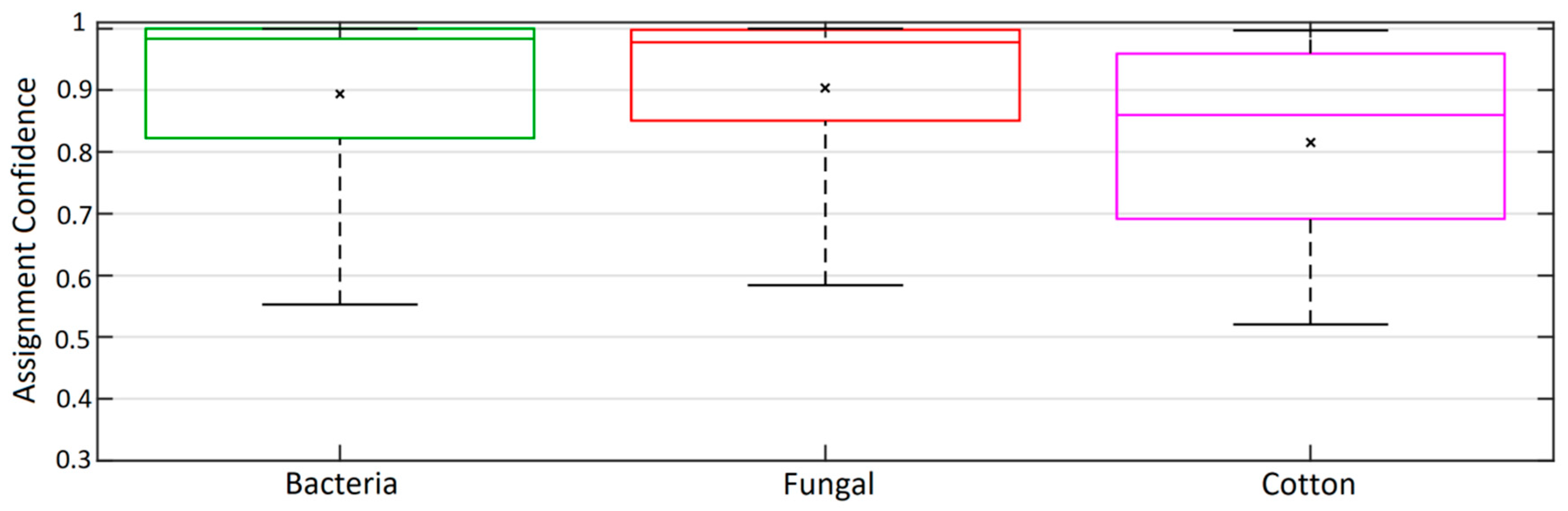
3.2. GBA Classification

First we train the GBA model using broad classes to generate products which are representative of bacteria, fungal spores and clothing fibres. Table 2 shows a confusion matrix assessing the performance of the model where it can be seen that the model performs exceptionally well and can classify the test portion of the input data to the model accurately.
We now apply the trained model to the ambient data collected at University Place. Figure 4 shows the classification assignment confidence (p) for each broad class as determined by the Scikit-learn GBA classifier. The GBA model will make a preliminary assignment for each fluorescent particle to one of the three classes based on the internally calculated assignment confidence; as there are only three classes the minimum confidence to make this preliminary assignment is therefore p > 1/3. At low confidence values misattribution due to inter-class conflation or the erroneous assignment of an unknown or untrained particle type to a class is likely. To minimise this, it is necessary to apply a minimum assignment confidence threshold when classifying particles for further analysis. Generally we observe that bacteria- and fungal-like particle classifications are judged to have been made with high confidence by the model with mean p values of approximately 0.9 ± 0.15 for each and with a significant proportion of each class being assigned with a confidence greater than 0.75. Due to their more heterogeneous characteristics, cotton fibres are less confidently assigned. All classes feature a large proportion in assignment confidence approaching 1, suggesting that the sampled particles match the distinctly different characteristics of the laboratory data well. We therefore employ a conservative threshold p value of 0.9 when integrating data products for each class to ensure that the selected particles are representative of the training data with minimal conflation and misattribution likely.
To further evaluate the performance and validity of the ambient GBA classifications, we use the Hellinger distance metric to compare group properties with those from the laboratory training data to assess similarity and potential inter-class conflation. Figure 5 shows the parameter Hellinger distances for each class compared to the class training data and other ambient classes (ambient p < 0.9); it can be seen that the bacterial class compares well to the training data and that it also displays significant differences to the other ambient classes across all parameters; the fungal classification displays differences to the training data fluorescent spectra, but a high level of morphological similarity. While no obvious conflation with the other classes was observed there was some morphological similarity to the cotton class; the cotton-like morphology compares well to the training data but there are differences in the fluorescent spectra, suggesting that textile fibres may be difficult to classify given their variable nature.
We now delve deeper into the comparison between the ambient classifications and training data by investigating the parameter distributions to attempt to understand the differences highlighted by the initial Hellinger distance analysis. Figure 6 shows the normalised ambient and training values of the parameters for each class, where the fluorescent spectra are sum normalised (as is input to the GBA model) and the remaining parameters are range scaled to the maximum possible expected value. In agreement with the Hellinger distance analysis, it can be seen that the distributions of parameters are in good agreement for the bacterial class, suggesting those particles assigned to this class match the characteristics of the bacterial training data very well.
The ambient fungal class shows reasonable agreement in the CMOS parameter space but displays fluorescence in the upper channels not observed in the training data. However, both display modal fluorescence in the 3rd channel (414 nm). This suggests that either:
  • The training data are not representative of ambient fungal spore fluorescence due to how they are produced and aerosolized. As noted earlier, the fungal material used in this study is intended for allergenic testing use and has undergone chemical processing by the manufacturer. This may impact their fluorescent and morphological characteristics.
  • That ambient fungal fluorescence is significantly altered by external factors.
  • That we observed a fluorescent particle type with similar morphological properties to the ACS fungal material particles which are not fully representative of building mycology resulting in conflation/misattribution. The training dataset used in this study does not contain all of the most commonly observed fungal particles in building mycology studies (e.g., Aspergillius and Penicillium species [15]) which may exhibit different autofluorescent characteristics to the training samples.
Finally we note that the cotton class is somewhat similar to the training data given its high variability, displaying a similar spectral shape and morphological parameters.

3.3. Ambient Indoor Air Time Series Product Analysis

We calculate 5 min integrated data products using a conservative assignment confidence threshold of p > 0.9 to minimize misclassification when interrogating the fluorescent aerosol population as discussed earlier. We also employ a second less strict threshold of p > 0.75 with the aim of increasing the retained population without introducing significant misattribution. Caution must be taken when interpreting products derived using this lower threshold, especially if the inclusion of additional particles results in significant differences in product trends when compared to the conservative threshold. Particles that fall outside of the scope of the training data should be assigned to one of the classes with a p value significantly below these thresholds and are thus excluded from any generated integrated data products. It may be possible to use intermediate p values to investigate particle novelty and underlying trends (i.e., displaying some broad characteristics which are similar to the training data) but caution must be taken interpreting products when doing so, and the resulting analysis must be caveated appropriately.
Figure 7 shows a time series of the integrated number concentrations for each class for the whole measurement period. Generally low background PBAP concentrations (a few per litre for all classes) are observed over the weekend when human activity inside University Place is low; weekdays display a consistent diurnal trend in the fungal-and cotton-like products, featuring a maximum around midday (approximately 80 L−1 and 10 L−1, respectively) which coincides with high activity inside the building as people use the catering facilities and enter and exit to attend lectures. Bacteria-like concentrations are elevated when compared to the weekend but the overall features of the weekday trends are less uniform. Several episodic bacterial events are observed with some major events occurring outside of the building public opening times. For example, Figure 8 shows a 12 h period from Friday the 13th of March which highlights this episodic behaviour; a relatively large and protracted bacteria-like event (~30 L−1) compared to background levels is observed between 7 and 8 AM, prior to any significant footfall inside the building. This then decays to near background levels before another, shorter-lived event (~55 L−1) is observed at around 9:30 AM. A final bacterial event (35 L−1) is observed at around 12:30 PM. Generally, these bacterial events do not correspond to enhancements in the fungal- and cotton-like classes.
Fungal-like particles display a macro-trend within the larger diurnal trend described earlier, where rapidly decaying spikes in number concentration are observed around the hour where footfall is high as people enter and exit the building to attend lectures and other events. Similar trends are also observed in the cotton-like class and this phenomenon is seen throughout the other weekdays.
Figure 9 shows the weekday hourly averaged diurnal number concentration for each class. This further highlights the diurnal trend in fungal-and cotton-like aerosol, both of which display an approximate midday maxima and little at night in synchronicity with human activity. This is highly suggestive that fungal-and cotton-like emissions are linked to human activity within the building which is consistent with previous studies [20]. Bacteria-like aerosols also display elevated concentrations during public opening hours and reduced background concentrations in the early hours of the morning. While we cannot say for certain what the underlying mechanisms for these emissions are, we speculate that human activity may disturb fungal particles through agitation/airflow causing aerosolization or may result in the resuspension of deposited bio-material and textile particles. Bacteria-like concentrations are also clearly elevated during periods of human activity; this result is consistent with that of Handorean et al., [19] which suggested that bacteria may be liberated from agitated textiles, which is a feasible emission mechanism at the site here. However, other unidentified mechanisms also may be at play as significant emission events occur outside of public opening hours. We now turn our attention to the remaining fluorescent population which have not been classified by the GBA model. We define the unclassified concentration as the difference between the total 9σ fluorescent concentration and the sum of the classified product concentrations (p > 0.9). It can be seen that the unclassified population generally displays a similar diurnal trend to the fungal and cotton classes. This suggests that the emission of a significant proportion of the unclassified fluorescent aerosol is related to human activity. The midday maxima of approximately 30 L−1 represents approximately 1/3rd of the fluorescent population at midday; this is a significant fraction of the population to remain unclassified. Broadening the scope of the training data to include fungal samples which are more broadly representative of building mycology and other human activity derived PBAP (e.g., skin flakes in dust) should improve the fraction of the fluorescent population which can successfully be classified. These will require further investigation.

4. Conclusions

In this manuscript, we demonstrate the utility of gradient boosting ensemble decision trees to classify and quantify PBAP in an indoor environment at high time resolution using a MBS UV-LIF spectrometer. We provide a framework to evaluate the quality of predictive outputs of supervised models by comparing input parameters to training data samples using Hellinger distance as a measure of similarity. This method also serves as a useful test to check if training sample sets are sufficiently different in characteristics to be reasonably separated using machine learning techniques. Additionally, we show the importance of comparing classified ambient and training data parameter distributions to evaluate confidence in the classification scheme and to highlight potential deficiencies in the training data used for a given ambient dataset. The following key results are highlighted:
  • We demonstrate that the GBA classification model can accurately classify the training data into broad PBAP classes.
  • The advanced CMOS shape information was demonstrated to be useful for minimising conflation between particle types with similar fluorescent characteristics but differing morphologies (e.g., E. coli bacteria and fungi).
  • The Hellinger distance metric framework displays a high level of utility for assessing both the likelihood of training data conflations (e.g., bacteria samples display similarity) and the applicability of the training data to generate an appropriate model for a given ambient dataset.
  • Some deficiencies in the fungal training samples were found using the above framework. They may arise due to either characteristic changes introduced by processing during manufacture or because the samples did not adequately represent the building mycology. This highlights the need to appraise the applicability of training data used to generate a classification model to build confidence in data outputs.
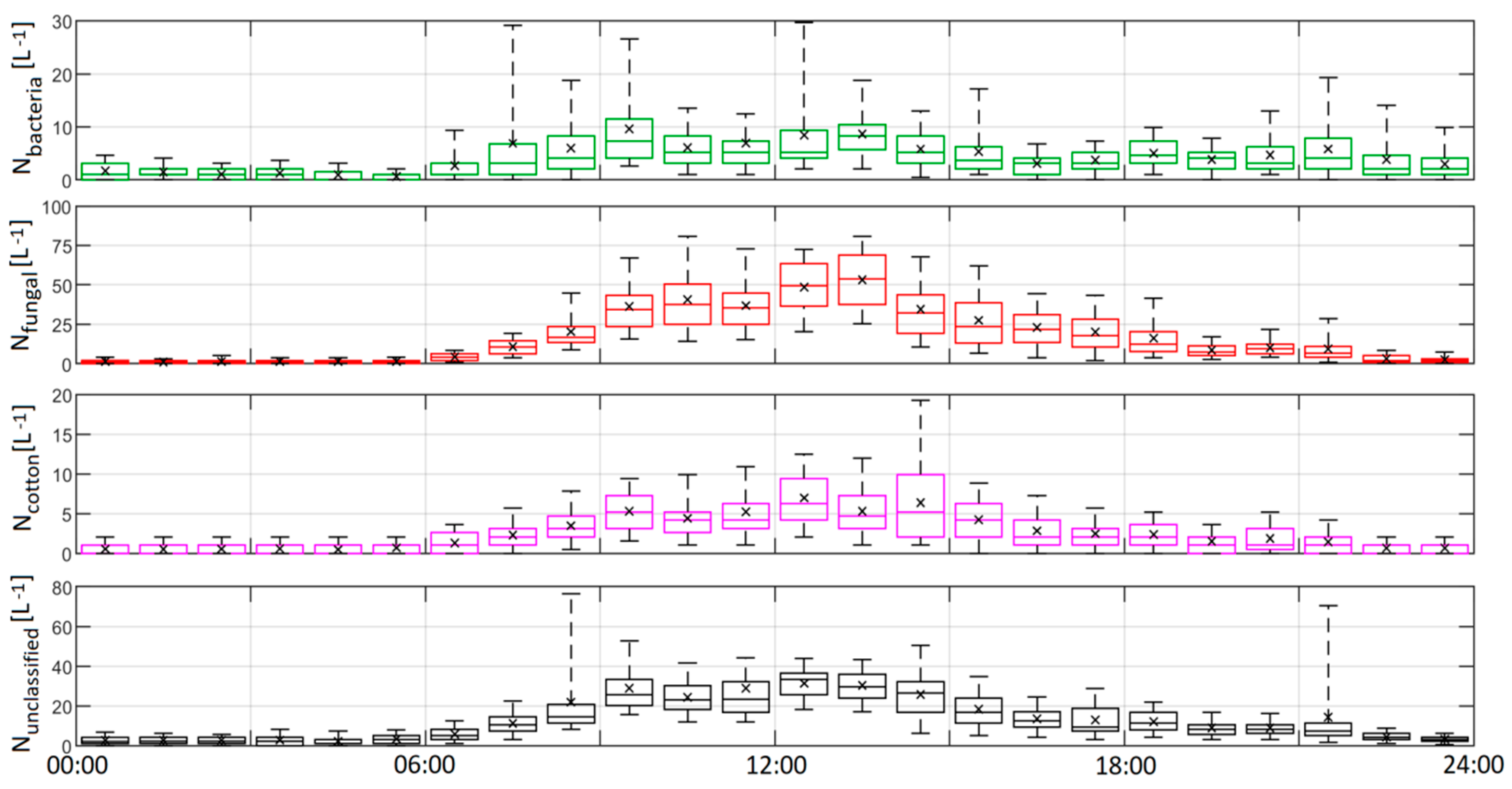
  • The application of the model to ambient indoor data yielded illuminating results about PBAP within the building investigated; bacteria-like aerosol were well captured by the training data and they exhibited a strong, yet episodic and complex response to human activity within the building; fungal-like aerosol were observed to display a strong diurnal response to human activity with maximum concentrations at midday, correlating to a maximum in footfall. Interestingly large, rapidly decaying spikes in concentration were observed around the hour, corresponding with a high flux of people through the building. Concentrations of all classes fell to baseline minimums when the building was closed.
  • High time resolution UV-LIF spectrometers can potentially reveal trends and mechanisms which may be obfuscated by offline methods that require long sample collections times.
Future work is planned to repeat this pilot study with a selection of cutting-edge high resolution UV-LIF spectrometers with supporting offline parallel analyses using microscopy, DNA sequencing and Q-PCR techniques to validate measurements and provide further insight into the identity and sources of PBAP constituents. The offline speciation will be used to inform further laboratory characterisation studies to generate appropriate training datasets to build updated GBA classification models. The work presented here demonstrates the utility of UV-LIF spectrometers and machine learning to assess PBAP impact on indoor air quality and exposure. The use of specialised training data focused on indoor bioaerosol composition in conjunction with high resolution, multiparameter UV-LIF spectrometers should significantly improve classification capability, providing excellent high temporal resolution datasets to interrogate PBAP emission mechanisms and evaluate impacts on air quality and exposure and eventually, emission and dispersion mitigation strategies.

Author Contributions

Conceptualization, I.C., M.G. and D.T.; software, I.C. and D.T.; formal analysis, I.C.; investigation, I.C., D.T. and M.G.; resources, M.G., V.F. and P.K.; data curation, E.F. and I.C.; writing—original draft preparation, I.C., M.G., D.T., J.R.L. and C.S.; visualization, I.C.; funding acquisition, M.G. and D.T. All authors have read and agreed to the published version of the manuscript.

Funding

This work was supported by NERC BIOARC programme, grant number NE/S002049/1. E.F. is funded under the Dstl (Defence Science and Technology Laboratory) and DGA (Direction Générale de l’Armement) Anglo-French PhD scheme (Grant reference DSTLX-1000120837) and affiliated to the NERC EAO Doctoral Training Partnership.

Conflicts of Interest

The authors declare no conflict of interest.

Abbreviations

The following abbreviations are used in this manuscript:
ACSAerosol challenge simulator
BGBacillus atrophaeus
BTBacillus thuringensis
CMOSComplementary metal-oxide-semiconductor
DstlDefence science and technologyl
FTForced trigger
GBAGradient boosting ensemble decision trees
HACHierarchical agglomerative clustering
MBSMultiparameter Bioaerosol Spectrometer
PBAPPrimary biological aerosol particle
UV-APSUltraviolet aerodynamic particle sizer
UV-LIFUltraviolet light-induced fluorescence
WIBSWideband integrated bioaerosol spectrometer

References

  1. Bauer, H.; Kasper-Giebl, A.; Löflund, M.; Giebl, H.; Hitzenberger, R.; Zibuschka, F.; Puxbaum, H. The contribution of bacteria and fungal spores to the organic carbon content of cloud water, precipitation and aerosols. Atmos. Res. 2002, 64, 109–119. [Google Scholar] [CrossRef]
  2. Bauer, H.; Schueller, E.; Weinke, G.; Berger, A.; Hitzenberger, R.; Marr, I.L.; Puxbaum, H. Significant contributions of fungal spores to the organic carbon and to the aerosol mass balance of the urban atmospheric aerosol. Atmos. Environ. 2008, 42, 5542–5549. [Google Scholar] [CrossRef]
  3. Möhler, O.; Georgakopoulos, D.G.; Morris, C.E.; Benz, S.; Ebert, V.; Hunsmann, S.; Saathoff, H.; Schnaiter, M.; Wagner, R. Heterogeneous ice nucleation activity of bacteria: New laboratory experiments at simulated cloud conditions. Biogeosciences 2008, 5, 1425–1435. [Google Scholar] [CrossRef] [Green Version]
  4. Crawford, I.; Bower, K.N.; Choularton, T.W.; Dearden, C.; Crosier, J.; Westbrook, C.; Capes, G.; Coe, H.; Connolly, P.J.; Dorsey, J.R.; et al. Ice formation and development in aged, wintertime cumulus over the UK: Observations and modelling. Atmos. Chem. Phys. 2012, 12, 4963–4985. [Google Scholar] [CrossRef] [Green Version]
  5. Morris, C.E.; Conen, F.; Alex Huffman, J.; Phillips, V.; Pöschl, U.; Sands, D.C. Bioprecipitation: A feedback cycle linking earth history, ecosystem dynamics and land use through biological ice nucleators in the atmosphere. Glob. Chang. Biol. 2014, 20, 341–351. [Google Scholar] [CrossRef] [Green Version]
  6. Huffman, J.A.; Prenni, A.J.; DeMott, P.J.; Pöhlker, C.; Mason, R.H.; Robinson, N.H.; Fröhlich-Nowoisky, J.; Tobo, Y.; Després, V.R.; Garcia, E.; et al. High concentrations of biological aerosol particles and ice nuclei during and after rain. Atmos. Chem. Phys. 2013, 13, 6151–6164. [Google Scholar] [CrossRef] [Green Version]
  7. Taylor, P.E.; Flagan, R.C.; Valenta, R.; Glovsky, M.M. Release of allergens as respirable aerosols: A link between grass pollen and asthma. J. Allergy Clin. Immunol. 2002, 109, 51–56. [Google Scholar] [CrossRef]
  8. Polymenakou, P.N.; Mandalakis, M.; Stephanou, E.G.; Tselepides, A. Particle Size Distribution of Airborne Microorganisms and Pathogens during an Intense African Dust Event in the Eastern Mediterranean. Environ. Health Perspect. 2008, 116, 292–296. [Google Scholar] [CrossRef] [Green Version]
  9. Fisher, M.C.; Henk, D.A.; Briggs, C.J.; Brownstein, J.S.; Madoff, L.C.; McCraw, S.L.; Gurr, S.J. Emerging fungal threats to animal, plant and ecosystem health. Nature 2012, 484, 186–194. [Google Scholar] [CrossRef]
  10. Ebbehoj, N.E.; Hansen, M.O.; Sigsgaard, T.; Larsen, L. Building-related symptoms and molds: A two-step intervention study. Indoor Air 2002, 12, 273–277. [Google Scholar] [CrossRef]
  11. Zeliger, H.I. Toxic Effects of Chemical Mixtures. Arch. Environ. Health Int. J. 2003, 58, 23–29. [Google Scholar] [CrossRef]
  12. Nag, P.K. Sick Building Syndrome and Other Building-Related Illnesses. In Office Buildings; Springer: Singapore, 2019; pp. 53–103. [Google Scholar]
  13. Netuveli, G.; Hurwitz, B.; Levy, M.; Fletcher, M.; Barnes, G.; Durham, S.R.; Sheikh, A. Ethnic variations in UK asthma frequency, morbidity, and health-service use: A systematic review and meta-analysis. Lancet 2005, 365, 312–317. [Google Scholar] [CrossRef]
  14. Tackling the Allergy Crisis in Europe—Concerted Policy Action Needed. Available online: http://www.eaaci.org/documents/EAACI_Advocacy_Manifesto.pdf (accessed on 20 July 2020).
  15. Haleem Khan, A.A.; Mohan Karuppayil, S. Fungal pollution of indoor environments and its management. Saudi J. Biol. Sci. 2012, 19, 405–426. [Google Scholar] [CrossRef] [PubMed] [Green Version]
  16. Sailer, M.F.; van Nieuwenhuijzen, E.J.; Knol, W. Forming of a functional biofilm on wood surfaces. Ecol. Eng. 2010, 36, 163–167. [Google Scholar] [CrossRef]
  17. Doherty, W.O.S.; Mousavioun, P.; Fellows, C.M. Value-adding to cellulosic ethanol: Lignin polymers. Ind. Crops Prod. 2011, 33, 259–276. [Google Scholar] [CrossRef] [Green Version]
  18. Feazel, L.M.; Baumgartner, L.K.; Peterson, K.L.; Frank, D.N.; Harris, J.K.; Pace, N.R. Opportunistic pathogens enriched in showerhead biofilms. Proc. Natl. Acad. Sci. USA 2009, 106, 16393–16399. [Google Scholar] [CrossRef] [Green Version]
  19. Handorean, A.; Robertson, C.E.; Harris, J.K.; Frank, D.; Hull, N.; Kotter, C.; Stevens, M.J.; Baumgardner, D.; Pace, N.R.; Hernandez, M. Microbial aerosol liberation from soiled textiles isolated during routine residuals handling in a modern health care setting. Microbiome 2015, 3, 72. [Google Scholar] [CrossRef] [Green Version]
  20. Bhangar, S.; Adams, R.I.; Pasut, W.; Huffman, J.A.; Arens, E.A.; Taylor, J.W.; Bruns, T.D.; Nazaroff, W.W. Chamber bioaerosol study: Human emissions of size-resolved fluorescent biological aerosol particles. Indoor Air 2016, 26, 193–206. [Google Scholar] [CrossRef] [Green Version]
  21. Huffman, J.A.; Perring, A.E.; Savage, N.J.; Clot, B.; Crouzy, B.; Tummon, F.; Shoshanim, O.; Damit, B.; Schneider, J.; Sivaprakasam, V.; et al. Real-time sensing of bioaerosols: Review and current perspectives. Aerosol Sci. Technol. 2020, 54, 465–495. [Google Scholar] [CrossRef] [Green Version]
  22. Ruske, S.; Topping, D.O.; Foot, V.E.; Kaye, P.H.; Stanley, W.R.; Crawford, I.; Morse, A.P.; Gallagher, M.W. Evaluation of machine learning algorithms for classification of primary biological aerosol using a new UV-LIF spectrometer. Atmos. Meas. Tech. 2017, 10, 695–708. [Google Scholar] [CrossRef] [Green Version]
  23. Forde, E.; Gallagher, M.; Walker, M.; Foot, V.; Attwood, A.; Granger, G.; Sarda-Estève, R.; Stanley, W.; Kaye, P.; Topping, D. Intercomparison of Multiple UV-LIF Spectrometers Using the Aerosol Challenge Simulator. Atmosphere 2019, 10, 797. [Google Scholar] [CrossRef] [Green Version]
  24. Könemann, T.; Savage, N.; Klimach, T.; Walter, D.; Fröhlich-Nowoisky, J.; Su, H.; Pöschl, U.; Huffman, J.A.; Pöhlker, C. Spectral Intensity Bioaerosol Sensor (SIBS): An instrument for spectrally resolved fluorescence detection of single particles in real time. Atmos. Meas. Tech. 2019, 12, 1337–1363. [Google Scholar] [CrossRef] [Green Version]
  25. Šaulienė, I.; Šukienė, L.; Daunys, G.; Valiulis, G.; Vaitkevičius, L.; Matavulj, P.; Brdar, S.; Panic, M.; Sikoparija, B.; Clot, B.; et al. Automatic pollen recognition with the Rapid-E particle counter: The first-level procedure, experience and next steps. Atmos. Meas. Tech. 2019, 12, 3435–3452. [Google Scholar] [CrossRef] [Green Version]
  26. Huffman, J.A.; Treutlein, B.; Pöschl, U. Fluorescent biological aerosol particle concentrations and size distributions measured with an Ultraviolet Aerodynamic Particle Sizer (UV-APS) in Central Europe. Atmos. Chem. Phys. 2010, 10, 3215–3233. [Google Scholar] [CrossRef] [Green Version]
  27. Gabey, A.M.; Vaitilingom, M.; Freney, E.; Boulon, J.; Sellegri, K.; Gallagher, M.W.; Crawford, I.P.; Robinson, N.H.; Stanley, W.R.; Kaye, P.H. Observations of fluorescent and biological aerosol at a high-altitude site in central France. Atmos. Chem. Phys. 2013, 13, 7415–7428. [Google Scholar] [CrossRef] [Green Version]
  28. Crawford, I.; Ruske, S.; Topping, D.O.; Gallagher, M.W. Evaluation of hierarchical agglomerative cluster analysis methods for discrimination of primary biological aerosol. Atmos. Meas. Tech. Discuss. 2015, 8, 7303–7333. [Google Scholar] [CrossRef]
  29. Forde, E.; Gallagher, M.; Foot, V.; Sarda-Esteve, R.; Crawford, I.; Kaye, P.; Stanley, W.; Topping, D. Characterisation and source identification of biofluorescent aerosol emissions over winter and summer periods in the United Kingdom. Atmos. Chem. Phys. 2019, 19, 1665–1684. [Google Scholar] [CrossRef] [Green Version]
  30. Savage, N.J.; Huffman, J.A. Evaluation of a hierarchical agglomerative clustering method applied to WIBS laboratory data for improved discrimination of biological particles by comparing data preparation techniques. Atmos. Meas. Tech. 2018, 11, 4929–4942. [Google Scholar] [CrossRef] [Green Version]
  31. Gabey, A.M.; Gallagher, M.W.; Whitehead, J.; Dorsey, J.R.; Kaye, P.H.; Stanley, W.R. Measurements and comparison of primary biological aerosol above and below a tropical forest canopy using a dual channel fluorescence spectrometer. Atmos. Chem. Phys. 2010, 10, 4453–4466. [Google Scholar] [CrossRef] [Green Version]
  32. Toprak, E.; Schnaiter, M. Fluorescent biological aerosol particles measured with the Waveband Integrated Bioaerosol Sensor WIBS-4: Laboratory tests combined with a one year field study. Atmos. Chem. Phys. 2013, 13, 225–243. [Google Scholar] [CrossRef] [Green Version]
  33. O’Connor, D.J.; Healy, D.A.; Hellebust, S.; Buters, J.T.M.; Sodeau, J.R. Using the WIBS-4 (Waveband Integrated Bioaerosol Sensor) Technique for the On-Line Detection of Pollen Grains. Aerosol Sci. Technol. 2014, 48, 341–349. [Google Scholar] [CrossRef]
  34. Crawford, I.; Robinson, N.H.; Flynn, M.J.; Foot, V.E.; Gallagher, M.W.; Huffman, J.A.; Stanley, W.R.; Kaye, P.H. Characterisation of bioaerosol emissions from a Colorado pine forest: Results from the BEACHON-RoMBAS experiment. Atmos. Chem. Phys. 2014, 14, 8559–8578. [Google Scholar] [CrossRef] [Green Version]
  35. Perring, A.E.; Schwarz, J.P.; Baumgardner, D.; Hernandez, M.T.; Spracklen, D.V.; Heald, C.L.; Gao, R.S.; Kok, G.; McMeeking, G.R.; McQuaid, J.B.; et al. Airborne observations of regional variation in fluorescent aerosol across the United States. J. Geophys. Res. Atmos. 2015, 120, 1153–1170. [Google Scholar] [CrossRef]
  36. Gosselin, M.I.; Rathnayake, C.M.; Crawford, I.; Pöhlker, C.; Fröhlich-Nowoisky, J.; Schmer, B.; Després, V.R.; Engling, G.; Gallagher, M.; Stone, E.; et al. Fluorescent bioaerosol particle, molecular tracer, and fungal spore concentrations during dry and rainy periods in a semi-arid forest. Atmos. Chem. Phys. 2016, 16, 15165–15184. [Google Scholar] [CrossRef] [Green Version]
  37. Kaye, P.H.; Hirst, E.; Greenaway, R.S.; Ulanowski, Z.; Hesse, E.; DeMott, P.J.; Saunders, C.; Connolly, P. Classifying atmospheric ice crystals by spatial light scattering. Opt. Lett. 2008, 33, 1545. [Google Scholar] [CrossRef] [PubMed]
  38. Savage, N.; Krentz, C.; Könemann, T.; Han, T.T.; Mainelis, G.; Pöhlker, C.; Huffman, J.A. Systematic Characterization and Fluorescence Threshold Strategies for the Wideband Integrated Bioaerosol Sensor (WIBS) Using Size-Resolved Biological and Interfering Particles. Atmos. Meas. Tech. Discuss. 2017, 1–41. [Google Scholar] [CrossRef] [Green Version]
  39. Freund, Y.; Schapire, R.E. A desicion-theoretic generalization of on-line learning and an application to boosting. In Lecture Notes in Computer Science; Springer: Berlin/Heidelberg, Germany, 1995; pp. 23–37. [Google Scholar]
  40. Hernandez, M.; Perring, A.E.; McCabe, K.; Kok, G.; Granger, G.; Baumgardner, D. Chamber catalogues of optical and fluorescent signatures distinguish bioaerosol classes. Atmos. Meas. Tech. 2016, 9, 3283–3292. [Google Scholar] [CrossRef] [Green Version]
  41. Pollen Count Averages for Northwest England. Available online: https://www.worcester.ac.uk/documents/Pollen-Count-Averages-for-Northwest-England.pdf (accessed on 30 June 2020).
Figure 1. Schematic of the complementary metal-oxide-semiconductor (CMOS) array data and parameters derived from a 3 µm polystyrene latex sphere particle. (a) Raw intensity data from the left and right CMOS arrays. Array peak, mean and peakwidth values are indicated by dashed, dot-dashed and dotted lines, respectively. Horizontal black line indicates array midpoint; (b) Modulus of the element by element subtraction of the left and right arrays. The resultant sum is the AsymLR parameter; (c) Raw intensity of the top and bottom sections of the left CMOS array, starting from the middle of the array outwards; (d) Modulus of the element by element subtraction of the top and bottom sections of the left CMOS array. The resultant sum is the Mirror parameter.
Atmosphere 11 01039 g001
Figure 2. ACS training data overview. Shown are the probability density functions of the CMOS parameters (columns 1 to 4) and box and whisker plots of the autofluorescent spectrum (row 5) for E.coli (top row); Bacillus atrophaeus (BG, 2nd row); Bacillus thuringensis (BT, 3rd row); Altenaria (4th row); Cladisporium (5th row); and cotton fibres (6th row). Whiskers denote 5th and 95th percentiles. Cross denotes mean value.
Atmosphere 11 01039 g002
Figure 3. ACS training data Hellinger distances for each parameter. Top panel: inter-class comparison of the broad classes. Bottom panel: intra-class comparison of the three bacterial samples. The Hellinger distance metric quantifies the similarity between two probability distributions where values towards zero indicate similarity between distributions and a value of 1 indicated dissimilarity.
Atmosphere 11 01039 g003
Figure 4. Box and whisker plots of the GBA model prediction class assignment confidence applied to the University Place ambient MBS data. Whiskers denote the 5th and 95th percentiles. Cross denotes mean value.
Atmosphere 11 01039 g004
Figure 5. Comparison of inter-class similarity. Hellinger distances for each parameter comparing the ambient classes to one another and also to their respective ACS training data. Top: Bacteria-like; Middle: Fungal-like; Bottom: Cotton-like. Ambient data is selected using an assignment probability of p > 0.9.
Atmosphere 11 01039 g005
Figure 6. Comparison of training (blue) and ambient (orange) parameter distributions for each class. Top: Bacteria-like; Middle: fungal-like; Bottom: Cotton-like. Fluorescent spectra have been normalised by the total fluorescent intensity. All other parameters have been scaled to the maximum possible expected value. Whiskers denote 5th and 95th percentiles.
Atmosphere 11 01039 g006
Figure 7. Time series of broad class number concentrations for the entire measurement period (5 min integrations). Top: Bacteria-like; Middle: fungal-like; Bottom: cotton-like. Solid line denotes an assignment probability p > 0.9; dashed line p > 0.75. Blue shaded area indicates weekdays.
Atmosphere 11 01039 g007
Figure 8. Same as Figure 7, but for the period 06:00–18:00 on Friday the 13th of March 2020.
Atmosphere 11 01039 g008
Figure 9. Weekday hourly averaged diurnal number concentrations. Top: Bacteria-like; 2nd row: fungal-like; 3rd row: cotton-like; bottom: unclassified. Whiskers denote 5th and 95th percentiles. Cross denotes mean value.
Atmosphere 11 01039 g009
Table 1. Summary of training test aerosol, including source, sample processing, storage conditions, dispersal method, average size and morphology. Particle size was determined using an optical particle counter during the 2017 ACS characterisation experiments; see Forde et al., [23] for details. Details of any processing steps are provided in Section 3.1.
SampleOriginProcessingStorageDispersalSize (µm)Morphology
Escherichia coli (G−)Dstl stockRe-suspended in phosphate-buffered saline>5 °CMedical nebuliser1.3 ± 0.6rod-shaped
Bacillus atrophaeus (G+)Dstl stockRe-suspended in phosphate-buffered saline>5 °CMedical nebuliser1.4 ± 0.4rod-shaped
Bacillus thuringensis (G+)Dstl stockRe-suspended in phosphate-buffered saline>5 °CMedical nebuliser1.2 ± 0.6rod-shaped
Alternaria AlternariaStallergenes Greer Strain ATCC 11680acetone<0 °Ccompressed air1.9 ± 4.2fibrous
Cladosporium herbarumStallergenes Greer Strain ATCC 6506acetone<0 °Ccompressed air2.7 ± 3.0fibrous
CottonBlack T-ShirtnoneN/Amechanical agitationN/A-
Table 2. Confusion matrix of the GBA classification model using the ACS training data grouped into broad classes. The proportion of the model predicted labels (columns) are compared to the true label (rows) for each broad training class and presented as a percentage value.
Predicted Label
BacteriaFungalCotton
Bacteria100%0%0%
True labelFungal0%100%0%
Cotton0%0%100%

