1. Introduction
It is well known that atmospheric waves are one part of the ionosphere dynamics. They usually propagate at different heights of the Earth’s atmosphere, including those in the lower ionosphere [
1,
2,
3]. As a result, the dynamics of the lower ionosphere affect the energy exchange between the mesosphere and the lower thermosphere. The lower ionosphere is characterized by significant variations in the temperature and density of the neutral component, electron density, and intense vertical and horizontal motions [
4,
5,
6,
7,
8]. The study of this region is one of the most relevant problems in space plasma physics.
Internal gravity waves (IGWs) are a type of atmospheric wave that has been investigated for many decades. During that period, the main properties of IGWs were studied—such as IGW sources, specific features of propagation, and generation mechanisms. The results of experimental studies of atmospheric waves by different methods, as well as the modeling of their propagation in the ionosphere from terrestrial, atmospheric, and ionospheric sources, are reported in numerous publications. Since the entire scope of work on the subject cannot be reviewed, we refer to a few sources that cover various aspects of experimental and theoretical studies of waves in the ionosphere [
9,
10,
11,
12,
13,
14,
15].
The turbulence and atmospheric waves influence the parameters and properties of the lower ionosphere [
5]. It is important to determine the altitude of the turbopause, the region where turbulent mixing is replaced by the diffusion separation of gases. Above the turbopause, ambipolar diffusion influences the transport processes. Turbulent formations can be carried along altitude by vertical movements and atmospheric waves.
IGWs are effectively studied using many radiophysical methods, including either measuring in situ parameters of the ionized component or the IGW impact on the electromagnetic wave propagation in a wide frequency range. Lidar observation, airglow imaging, measurements of the horizontal wind by meteor radar, and satellite observation allow one to determine IGW vertical and horizontal parameters from the lower atmosphere to the thermosphere [
11,
12,
13,
14,
15]. Among these techniques, the method based on a scattering of high frequency radio waves by artificial periodic irregularities of the ionospheric plasma is promising [
8,
16,
17,
18,
19,
20,
21,
22,
23].
The aim of the present study is to demonstrate how atmospheric waves influence the temperature, density of the neutral component, and velocity of vertical regular motion of the ionosphere plasma at altitudes of the lower ionosphere. All the results were obtained by a method based on creating artificial periodic irregularities in ionospheric plasma by its disturbance with high-frequency radio emission from the Sura heating facility.
2. Data and Methods
The API technique is based on ionosphere perturbation by powerful high frequency radio emission, and the creation of periodic irregularities in the field of a standing wave formed by the reflection from the ionosphere of the powerful radio wave emitted by the heating facility to zenith. In the D-region (heights are 60–90 km), the main role in API formation is played by the temperature dependence of the coefficient of the electron attachment to neutral molecules. In the E-region (heights are 90–150 km), APIs are formed by the diffusion redistribution of the plasma under the influence of the excess pressure of the electron gas, and in the F-region (heights are 150–350 km), they arise under the action of the ponderomotive force on the ionosphere plasma. The powerful wave is always reflected in the F-region. Irregularities are formed at the height range from 50 to 60 km to the height of the powerful wave reflection from the ionosphere. The vertical scale of these irregularities is equal to half the wavelength emitted by transmitters of the heating facility in the plasmas. The API technique is based upon observations of the Bragg backscatter of the pulsed probe radio waves on the periodic irregularities. The API technique and methods of determination of many ionosphere parameters are presented in detail in [
8]. Many results of ionosphere studies by this method are given in [
16,
17,
18,
19,
20,
21,
22,
23,
24]. In this paper, we present the results of recent experiments on ionosphere studies by the API technique using the Sura heating facility.
The destruction (relaxation) of irregularities after the end of heating occurs under the impact of ambipolar diffusion in the E-region of the ionosphere, and due to the temperature dependence of the electron detachment coefficient in the D-region [
8]. The dependence of the API relaxation time on the ambipolar diffusion coefficient makes it possible to determine the temperature and the density of the neutral component of the ionosphere. To do this, the disturbed ionosphere region is probed by radio waves. The scattering of probe radio waves on artificial periodic irregularities has resonant properties; that is, the API scattered signal has significant amplitude with identical frequencies and polarizations of the powerful and probing radio waves. In the experiment, the amplitude and the phase of the API scattered signal are measured. By decreasing the amplitude of the scattered signal during the APIs disappearance, the relaxation time of irregularities is determined. In the lower part of the E-region of the ionosphere (90–120 km), where the effect of atmospheric turbulence can be ignored, the relaxation of irregularities in the E-layer is controlled by ambipolar diffusion, and the API relaxation time τ is determined by the expression
where
κ is the Boltzmann constant,
K = 4
π/λ is the wave number of the standing wave,
λ = λ0/n is the wavelength in the plasma,
D is the ambipolar diffusion coefficient,
M is the molecular mass of ions,
Te0 and
Ti0 are the background (unperturbed) electron and ion temperatures, and
νim is the frequency of collisions of ions with molecules. In the lower ionosphere
Te0 =
Ti0 =
T, where
T is the neutral temperature. The given expression for τ underlies the determination of most of the parameters of the lower ionosphere [
8,
16,
18,
24,
25,
26]. Temporal density variations repeat in general temperature variations. A detailed description of the method for determination of the neutral temperature and the density, derived from the height dependence of the relaxation time of the API scattered signal 104, and estimations of the method accuracy in determining the temperature and density in the lower ionosphere are in [
25,
26].
The plasma vertical velocity at altitudes of 50–130 km is equal to the velocity of the neutral component, due to the fact that the plasma at these altitudes behaves as a passive admixture. The plasma vertical velocity is found by the phase
φ change of the scattered signal as
where
f is the frequency of the powerful probe radio waves,
n is the refractive index, and
c is the light velocity in the vacuum. A positive value of the velocity corresponds to downward motion. In [
8], an estimate of the possible systematic error in determining the velocity is done. For the extraordinary wave used to create and locate the APIs, it does not exceed 0.05 m/s under ordinary ionosphere conditions. In [
8], it is proven that in a moving environment at the heights of the lower ionosphere, the created irregularities are attracted by the movement of a neutral gas in less than a millisecond during their relaxation. Therefore, measurement of the phase of the scattered signal gives the velocity of the vertical movement of the neutral component of the ionosphere at the indicated heights.
On the basis of Equations (1) and (2), the neutral temperature and density, the turbopause height, and the turbulent and the regular vertical velocity are estimated. Analysis of altitude-time dependences of the neutral temperature, the vertical plasma velocity, and other ionosphere and neutral atmosphere parameters allows one to investigate properties of the propagation of atmospheric waves.
3. Recent Experiments
We present results of resent experiments on the studies of the ionosphere and the neutral atmosphere by the API technique. All experiments were carried out using the Sura heating facility (56,15 N; 46,11 E) located near Nizhny Novgorod, Russia. To create APIs, the heating facility transmitters emitted continuously in phase the extraordinary wave with the effective radiated power of 80–120 MW at the frequency 4.7 (4.785) or 5.6 MHz for 3 or 5 s. After the end of the ionosphere disturbance, the heating facility emitted short pulses with duration at 30 µs and with a repetition rate of 50 Hz. During the pulses mode, the frequency and polarization were identical as that of the heating mode. The amplitudes and the phases of the backscattered signals were measured during the time when the heater was turned off. Thus, one measurement cycle lasted 15 s. The signals were recorded with the height step of 1.4 km and with time resolution of 15 s. We note that resonant type of the API scattering provides the true height resolution of about 1 km. Good spatial and time resolution are advantages of the API technique, and they enable studying the dynamic phenomena—including fast processes in the ionosphere and the neutral atmosphere. The API relaxation (decay) time was determined by the amplitude decrease of the scattered signal by a factor of e after turning off the powerful transmitter. We used the average values of the measured parameters on the time interval of 5 or 10 min.
The typical example of the amplitude and the phase of the API scattered signal is presented in
Figure 1. It shows the temporal-height plots of the amplitude and the phase of the API scattered signal during the relaxation process of irregularities. The API scattered signals in the D-, E-, and F-regions of the ionosphere and the sporadic E-layer are visible.
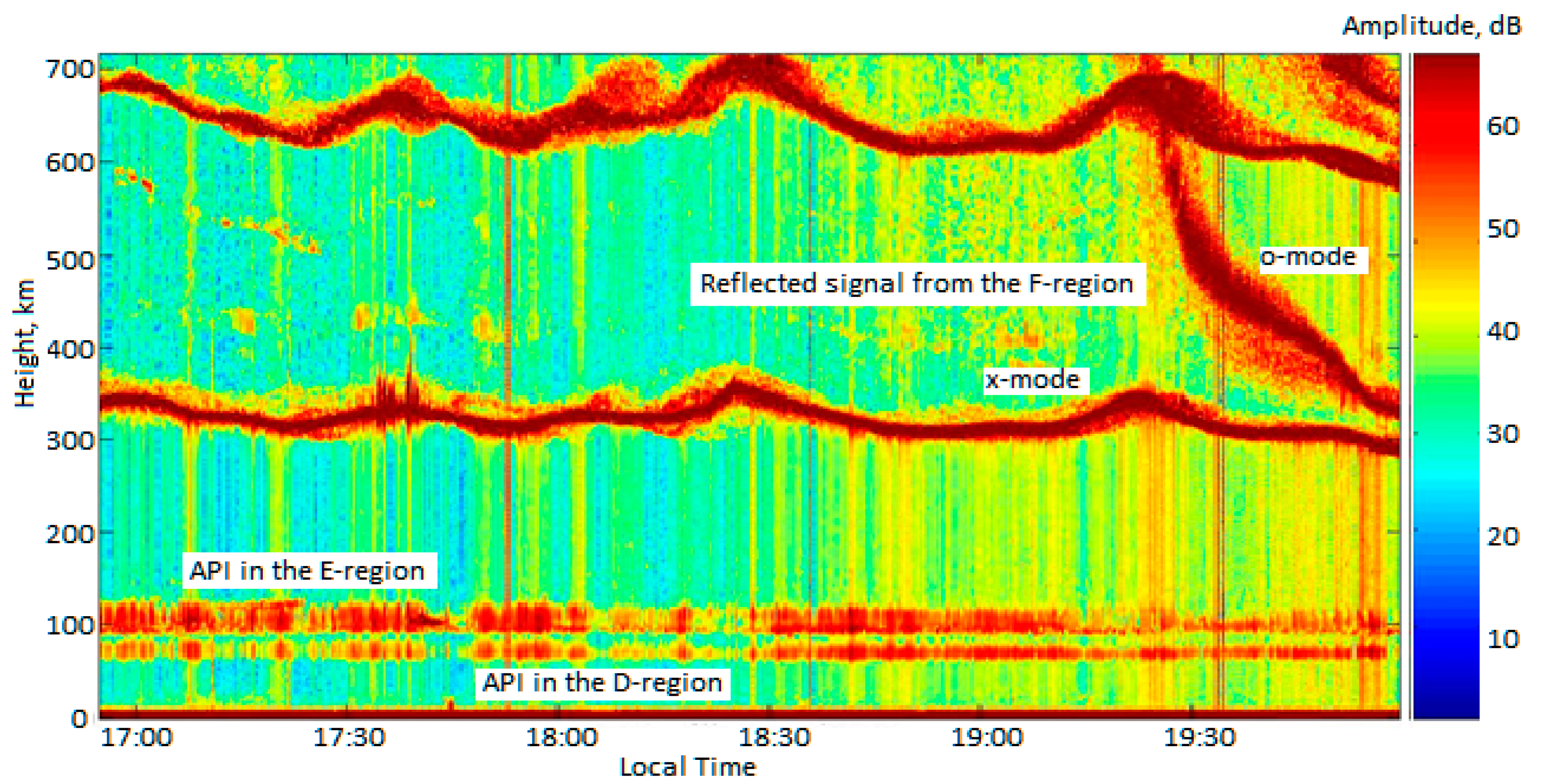
Figure 2 shows the time-height-amplitude plot of the API scattered signal obtained on 9 August 2017. The ionosphere signals reflected from natural regions of the ionization and API scattered signals in the D-, E-, and F-regions are visible.
The altitude range from 65 to 120 km in
Figure 2 is occupied by the scattered signal in the D- and E-regions. Just below 100 km, the signal from the sporadic E-layer is almost always visible. At the height of about 300–350 km, a specular reflection of the x-mode probing wave from the ionosphere F-region is shown. We note the o-mode of the probing wave was not reflected from the ionosphere until 19:30. Above 600 km, you can see the second reflection of the probe wave. Pay attention to the wavelike change in the height of the specula reflection.
4. Observation Results
We presented some examples of the API observations in the previous section. In this section we demonstrate and discuss the altitude and temporal variations of the relaxation time of the API scattered signal, and the vertical plasma velocity and variations of the neutral temperature and density.
4.1. API Relaxation Time and Vertical Plasma Velocity
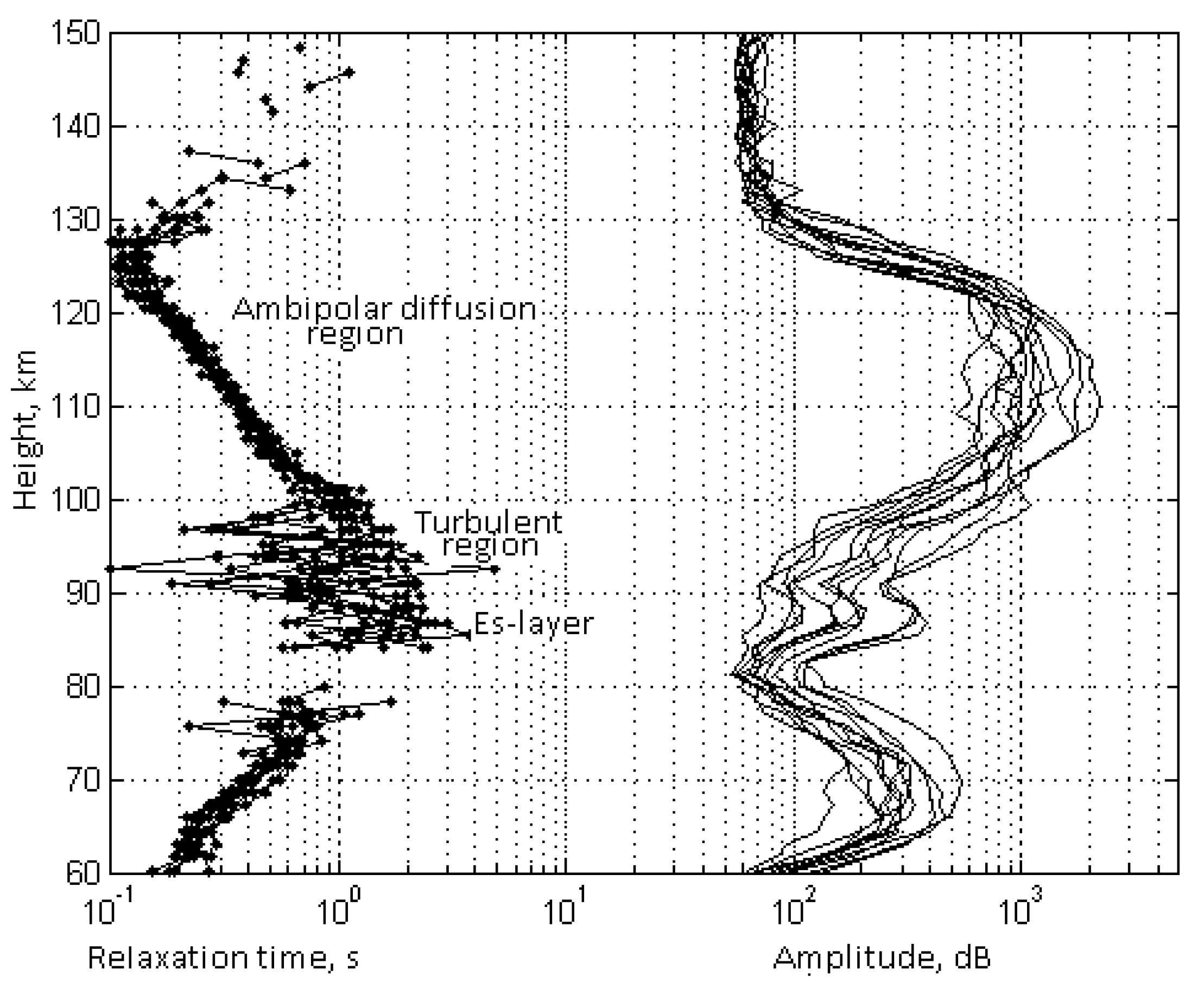
Height profiles of the API scattered signal characteristics as the relaxation time τ (left curves) and the amplitude A (right curves), obtained 30 September 2016 in session 13:54–13:58, are presented in
Figure 3. The API scattered signal amplitude reaches a maximum in the E-region, where the signal-to-noise ratio is 10:100. In this example, at the height range of 95–125 km, the API relaxation process occurs under the impact of ambipolar diffusion and values of relaxation times are in good agreement with the diffusion dependence τ(h). Below 100 km, atmospheric turbulence begins to impact on the relaxation process. Irregularities break down faster and the relaxation time of the scattered signal decreases as compared with the diffusion time. In the D-region, the amplitude and relaxation time change with height, in full accordance with the dependence detachment coefficient from the electron temperature [
8]. The pattern of the temporal variations of the relaxation time determines the corresponding variations in the temperature and density of the neutral component.
The anomalously low sporadic E-layer provides a local increase in the amplitude and relaxation time of the scattered signal at the altitude of 85 km. At the heights of the sporadic E-layer (90–100 km), the velocity drops to zero and changes direction. In most cases, a change in the direction of the velocity corresponds to the height of the maximum of the sporadic E (E
s)-layer ionization, which means the formation of the E
s-layer directly above the observation point because of the moving plasma redistribution o in the Earth’s magnetic field. Wind shear theory explains this phenomenon [
27,
28,
29].
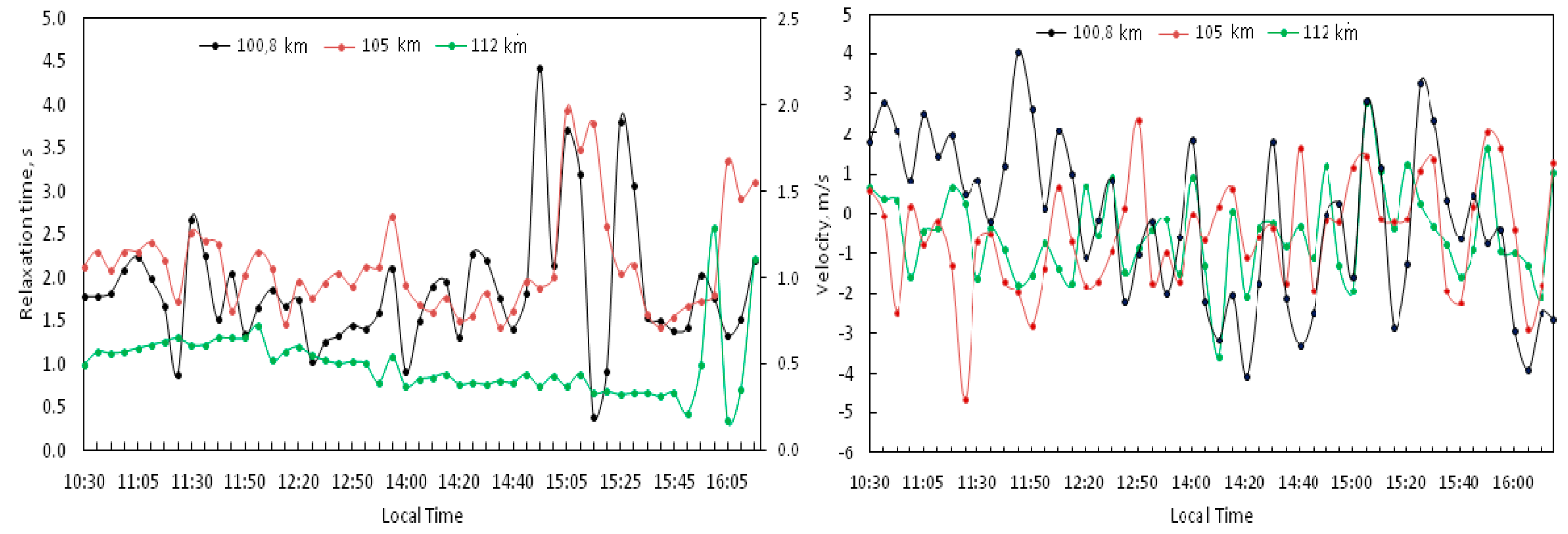
In
Figure 4, temporal variations of the API relaxation time and the vertical plasma velocity at the heights of 100.8 km, 105 km, and 112 km for 25 October 2018 are shown. The relaxation time decreases strongly as height increases, so the right vertical axis of coordinates is related to the green curve for convenience. It is seen that both the API relaxation time and the vertical plasma velocity present wavelike time variations. Elevated relaxation times appear when a sporadic E-layer exists during the observations [
8,
24,
30]. The existence of a sporadic layer during the experiments is confirmed by ionograms of vertical sounding of the CADI ionosonde at the location near the Sura facility [
30].
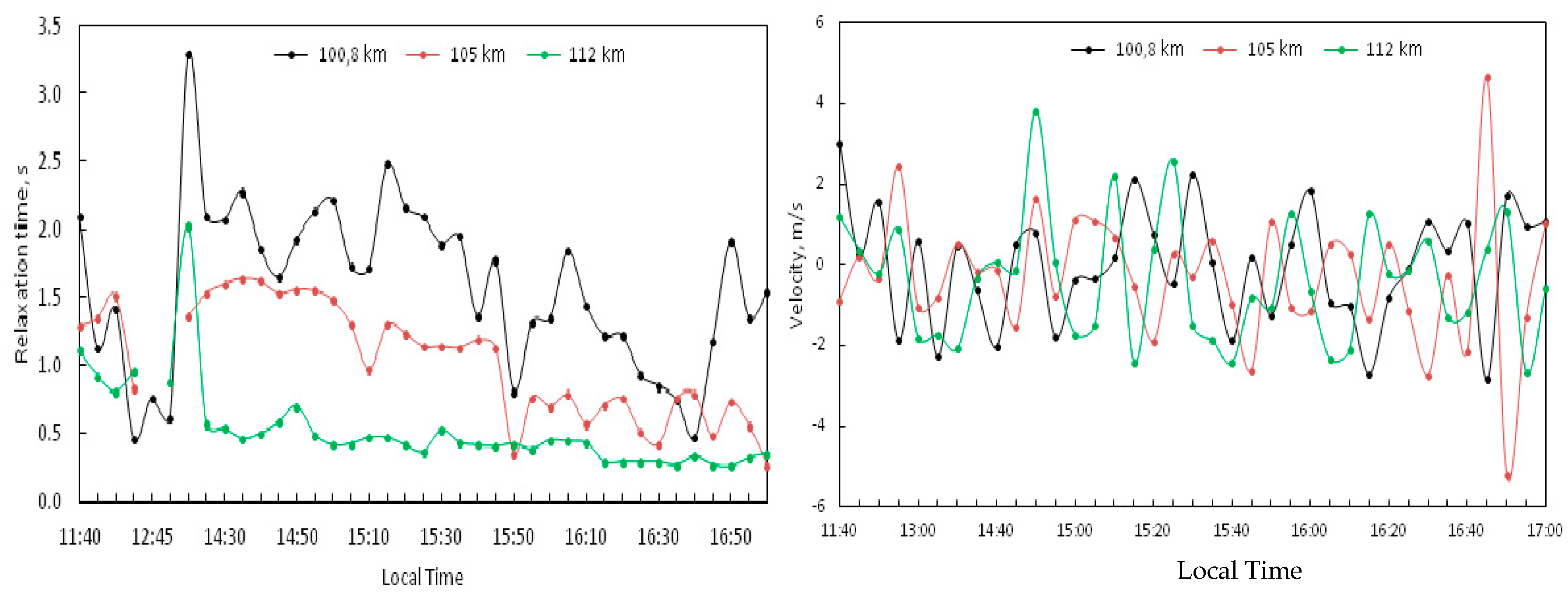
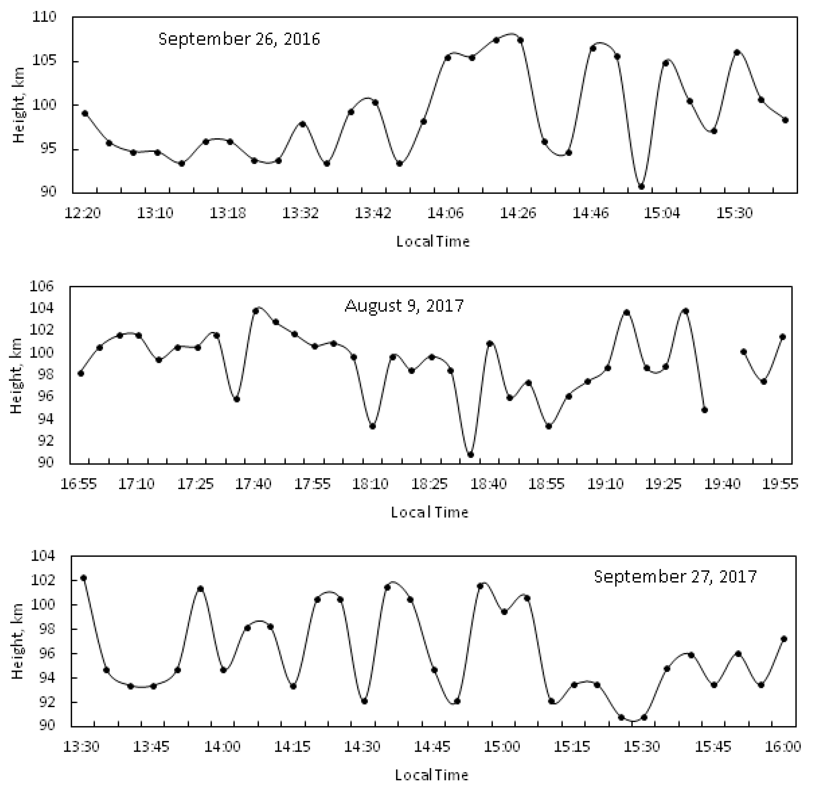
Similar variations of the relaxation time and the vertical plasma velocity are shown in
Figure 5 for 27 September 2017.
Figure 6 presents the temporal dependence of vertical plasma velocity values averaged over 5 min on 28 September 2018 for three heights of the E-region at 100 km, 105 km, and 112 km (left panel), and for the D-region at 66 km, 76 km, and 85 km (right panel).
In
Figure 6, significant wavelike velocity variations are visible at all altitudes in both the D- and E-regions. The average velocity ranged from −6 to +6 m/s in the lower part of the D-region, and from −3 to +5 m/s in the E-region. One can see undulating variations in the velocity with a constant change of direction and a period from 10 min to 1 h in the D-region, and up to 3 h in the E-region, which indicates the intensive dynamics in this height range.
4.2. Neutral Temperature and Turbopause Level
Expression (1) for the relaxation time of the API scattered signal is the basis for determining the temperature T and density ρ of the neutral component in the lower part of the E-region to an altitude of 120–130 km. The method of determining these parameters is described in detail in [
8]. In most experiments, wave variations in temperature and density were observed, often of an unstable nature [
18,
21,
31]. It was natural to assume that perturbations of this kind can be caused by the propagation of internal gravity waves. Clearly-pronounced wave movements with a period from 15 min to 2 h or more are clearly visible; there is a complex picture of temporal temperature variations with a range of oscillations from 20 to 100 K [
22,
25,
26,
31,
32].
The temporal dependencies of the temperature and the density of the neutral component of the lower ionosphere for two heights at 100 km and 105 km in daytime hours on 28 September 2018 are shown in
Figure 7. Clearly-pronounced wave movements with a period from 15 min to 2 h or more are clearly visible; there is a complex structure of temporal temperature variations with a range of oscillations from 20 to 100 K.
Waves with different periods of manifestation are in oscillations of the neutral temperature at the heights of 100 km and 105 km.
The turbopause level can be defined as a height in the ionosphere, below which turbulent mixing predominates, and molecular diffusion is dominant above it. Turbulent structures can be transported to the lower thermosphere by vertical motions and atmospheric waves. The turbopause level varies depending on the time of day. The method of turbopause level determination on the basis of the API technique is discussed in [
32]. API observations show that relaxation time decreases with increasing altitude, in accordance to the ambipolar diffusion law (
Figure 3). Below the turbopause level, turbulent mixing begins; this height we consider as the turbopause height. For example, in
Figure 8, variations of the turbopause height determined by this method for three days of the API observation are presented.
The turbopause level varied in range of heights of 92–108 km, detecting both relatively fast and slower variations. For example, on 27 September 2017, the level of the turbopause varied from 90 km to 102 km. Large-scale oscillations with a period of 105 min are overlaid on the wavelike variations of the turbopause level with a characteristic period of 15–20 min. Similar variations in the turbopause level were observed on other days.
5. Atmospheric Waves
Wavelike oscillations of the API relaxation time, the neutral temperature and the density, the vertical velocity, and turbopause level have periods of oscillations from several minutes to several hours. Such periods are characteristic of internal gravity waves and are their manifestation in the ionosphere and the neutral atmosphere parameters. The results of long-term measurements of the parameters of the neutral component and the plasma vertical velocity in the lower ionosphere by the API technique convincingly demonstrate a significant effect of atmospheric waves, which are most intense during natural disturbances [
16,
17,
33]. The amplitude of the waves can reach 50–100 K in temperature and up to 12–15 m/s in the vertical velocity value. Such waves can have a significant effect on the measurement results of the total electron content in the ionosphere. Changes in the turbopause level are characterized by quasi-periodicity with a period from 10 to 15 min to several hours, which may be due to the influence of internal gravity waves on the state of the ionosphere and the neutral atmosphere.
We give estimates of the characteristic period of the wave. The simplified dispersion equation of internal gravity waves (IGW) in the incompressible medium approximation can be represented as
where
is the Brunt-Väisälä frequency, and
are vertical and horizontal wavelengths. In the long-wave approximation,
<<
, we obtain
from Equation (3). In this case, the horizontal component of the phase velocity will be equal to
. This ratio is similar to that given by the velocity of long gravitational waves in shallow water [
34].
In another limiting case that is used often in the interpretation of natural TIDs (traveling ionospheric disturbances) in the ionosphere [
2,
35], as in our experiments [
8,
22], when the conditions
are fulfilled, we obtain the relation
from Equation (3). We denote the period of the wave
. For waves periods
and the period corresponding to the Brunt-Väisälä frequency
, this ratio gives
. If we take a period
= 5 min and
for the height of the lower thermosphere at 90–120 km, then the minimum period of the observed waves will be at least 15 min, namely
min. The results of determining the wave periods as presented in this paper, as well as in [
8,
22], are consistent with the estimate above.
We also note that the possibility of the IGW generating under special operating conditions of the powerful heating facility was analyzed in a number of works (see, for example, [
36]). Experimental results of the artificial IGW generation by heating facilities are presented in [
37,
38,
39].
The task of further studying the manifestations of atmospheric waves in the parameters of the ionosphere and the neutral atmosphere is a joint analysis of variations of the turbopause level and variations of the temperature of the neutral component, as well as vertical and turbulent motion velocities, determined by the API technique. Such an approach will make it possible to find out the conditions for the stability of the environment during the IGW propagation, to estimate the fraction of the energy transmitted by the waves to the propagation environment at different heights, and to reveal the contribution of the dissipation of wave energy to the increase in neutral temperature. It may be useful to compare the variations in temperature and level of the turbopause.
6. Conclusions
This paper presents the results of new experiments carried out in 2017–2018, including original results, to determine of the turbopause level, the neutral temperature and density, and plasma vertical velocity. The paper shows the possibility of studying atmospheric waves by creating artificial periodic irregularities. We obtained that turbopause level was located in the altitude range of 90–100 km, and plasma velocity in the altitude range of 60–120 km was determined. The average velocity ranged from −6 to +6 m/s in the lower part of the D-region, and from −3 to +5 m/s in the E-region. Significant wavelike velocity variations are visible at all altitudes in both D- and E-regions.
As in the works of the authors cited in the article, the manifestations of wave motions in variations of parameters of the neutral atmosphere and the vertical plasma velocity are demonstrated. The results of measurements of the characteristics of the API scattered signals, altitude and temporal variations of the neutral atmosphere temperature and the vertical plasma velocity, and the level of the turbopause can be used to study dynamic phenomena in the altitude range of 60–120 km. It was established that they are characterized by quasi-periodicity with a period from 10 to 15 min to several hours, which may be a manifestation of internal gravitational waves in the ionosphere and the neutral atmosphere.
Author Contributions
Conceptualization, N.V.B.; methodology, N.V.B. and A.V.T.; software, I.N.Z.; validation, N.V.B., A.V.T., and G.I.G.; formal analysis, N.V.B. and I.N.Z.; investigation, N.V.B., G.I.G., A.V.T., and I.N.Z.; resources, N.V.B.; data curation, N.V.B.; writing—original draft preparation, N.V.B.; writing—review and editing, N.V.B., G.I.G., and A.V.T.; visualization, N.V.B. and I.N.Z; project administration, N.V.B.
Funding
This research was supported by the Russian Foundation for Basic Research, grant number 18-05-00293, and the Ministry of Science and Higher Education of Russian Federation, grant number 5.8092.2017/8.9.
Acknowledgments
The authors thank E.E. Kalinina and G.V. Vinogradov for their participation in the carrying out of the API experiments, and assistance in the processing of the results of measurements obtained by the API technique.
Conflicts of Interest
The authors declare no conflict of interest. The funders had no role in the design of the study; in the collection, analyses, or interpretation of data; in the writing of the manuscript; or in the decision to publish the results.
References
- Gossard, E.E.; Hooke, W.H. Waves in the Atmosphere; Elsevier: Amsterdam, The Netherlands; New York, NY, USA, 1975; 456p. [Google Scholar]
- Hines, C.O. Internal atmospheric gravity waves at atmospheric heights. Can. J. Phys. 1960, 38, 1441–1481. [Google Scholar] [CrossRef]
- Fritts, D.C.; Alexander, M.J. Gravity waves dynamics and effects in the middle atmosphere. Rev. Geophys. 2003, 41, 1003. [Google Scholar] [CrossRef]
- Danilov, A.D.; Kalgin, U.A.; Pokhunkov, A.A. Variation of the turbopause level in the polar regions. Space Res. XIX 1979, 83, 173–176. [Google Scholar]
- Hocking, W.K. Dynamical coupling processes between the middle atmosphere and lower ionosphere. J. Atmos. Terr. Phys. 1996, 58, 735–752. [Google Scholar] [CrossRef]
- Kirkwood, S. Seasonal and tidal variations of neutral temperatures and densities in the high latitude lower thermosphere measured by EISCAT. J. Atmos. Terr. Phys. 1986, 48, 815–826. [Google Scholar] [CrossRef]
- Offermann, D.; Jarisch, M.; Oberheide, J.; Gusev, O.; Wohltmann, I.; Russel, J.M., III; Mlynczak, M.G. Global wave activity from upper stratosphere to lower thermosphere: A new turbopause concept. J. Atmos. Sol. Terr. Phys. 2006, 68, 1709. [Google Scholar] [CrossRef]
- Belikovich, V.V.; Benediktov, E.A.; Tolmacheva, A.V.; Bakhmet’eva, N.V. Ionospheric Research by Means of Artificial Periodic Irregularities; Copernicus GmbH: Katlenburg-Lindau, Germany, 2002; 160p. [Google Scholar]
- Grigoriev, G.I. Acoustic-gravity waves in the earth’s atmosphere (Review). Radiophys. Quanum Electron. 1999, 42, 1–21. [Google Scholar] [CrossRef]
- Vasilyev, P.A.; Karpov, I.V.; Kshevetskii, S.P. Modeling of the effect of internal gravity waves on upper atmospheric conditions during sudden stratospheric warming. Sol. Terr. Phys. 2016, 2, 99–105. [Google Scholar] [CrossRef]
- Chanin, M.L.; Hauchcorne, A. Lidar observationof gravity and tidal waves in the stratosphere and mesosphere. J. Geophys. Res. 1981, 86, 9715–9721. [Google Scholar] [CrossRef]
- Gong, S.; Yang, G.; Xu, J.; Liu, X.; Li, Q. Gravity wave propagation from the stratosphere into the mesosphere studied with lidar, meteor radar, and TIMED/SABER. Atmosphere 2019, 10, 81. [Google Scholar] [CrossRef]
- Gavrilov, N.M.; Fukao, S.; Nakamura, T.; Tsuda, T. Statistical analysis of gravity waves observed with the middle and upper atmosphere radar in the middle atmosphere: Method and general characteristics. J. Geophys. Res. 1996, 101, 29511–29521. [Google Scholar] [CrossRef]
- Tsuda, T.; Kato, S.; Yokol, T.; Inoue, T.; Yamamoto, M.; VanZand, T.E.; Fukao, S.; Sato, T. Gravity waves in the mesosphere observed with the middle and upper atmosphere radar. Radio Sci. 1990, 26, 1005–1018. [Google Scholar] [CrossRef]
- Nakamura, T.; Tsuda, T.; Yamamoto, M.; Fukao, S.; Kato, S. Characteristics of gravity waves in the mesosphere observed with the middle and upper atmosphere radar, 1&2. J. Geophys. Res. 1993, 98, 8899–8923. [Google Scholar]
- Bakhmetieva, N.V.; Bubukina, V.N.; Vyakhirev, V.D.; Kalinina, E.E.; Komrakov, G.P. Response of the lower ionosphere to the partial solar eclipses of August 1, 2008 and March 20, 2015 based on observations of radio-wave scattering by the ionospheric plasma irregularities. Radiophys. Quantum Electron. 2017, 59, 782–793. [Google Scholar] [CrossRef]
- Bakhmetieva, N.V.; Vyakhirev, V.D.; Kalinina, E.E.; Komrakov, G.P. Earth’s lower ionosphere during partial solar eclipses according to observations near Nizhny Novgorod. Geomagn. Aeron. 2017, 57, 58–71. [Google Scholar] [CrossRef]
- Grigor’ev, G.I.; Bakhmetieva, N.V.; Tolmacheva, A.V.; Kalinina, E.E. Relaxation time of artificial periodic irregularities of the ionospheric plasma and diffusion in the inhomogeneous atmosphere. Radiophys. Quantum Electron. 2013, 56, 187–196. [Google Scholar] [CrossRef]
- Bakhmetieva, N.V.; Grigor’ev, G.I.; Tolmacheva, A.V.; Kalinina, E.E.; Egerev, M.N. Internal gravity waves in the lower thermosphere with linear temperature profile: Theory and experiment. Radiophys. Quantum Electron. 2017, 60, 103–112. [Google Scholar] [CrossRef]
- Bakhmetieva, N.V.; Belikovich, V.V. Results of studying the sporadic E layer by the method of resonant scattering of radio waves by artificial periodic inhomogeneities of the ionospheric plasma. Radiophys. Quantum Electron. 2008, 51, 862–873. [Google Scholar] [CrossRef]
- Bakhmetieva, N.V.; Grigor’ev, G.I.; Tolmacheva, A.V. Artificial periodic irregularities, hydrodynamic instabilities, and dynamic processes in the mesosphere-lower thermosphere. Radiophys. Quantum Electron. 2011, 53, 623–637. [Google Scholar] [CrossRef]
- Bakhmetieva, N.V.; Belikovich, V.V.; Grigor’ev, G.I.; Tolmacheva, A.V. Effect of acoustic gravity waves on variations in the lower-ionosphere parameters as observed using artificial periodic inhomogeneities. Radiophys. Quantum Electron. 2002, 45, 211–219. [Google Scholar] [CrossRef]
- Bakhmetieva, N.V.; Grigor’ev, G.I.; Tolmacheva, A.V.; Kalinina, E.E. Atmospheric turbulence and internal gravity waves examined by the method of artificial periodic irregularities. Russ. J. Phys. Chem. B 2018, 12, 510–521. [Google Scholar] [CrossRef]
- Kagan, L.M.; Bakhmet’eva, N.V.; Belikovich, V.V.; Tolmacheva, A.V. Structure and dynamics of sporadic layers of ionization in the ionospheric E region. Radio Sci. 2002, 37, 1106–1123. [Google Scholar] [CrossRef]
- Tolmacheva, A.V.; Belikovich, V.V.; Kalinina, E.E. Atmospheric parameters measured using artificial periodic irregularities with different spatial dimensions. Geomagn. Aeron. 2009, 49, 239–246. [Google Scholar] [CrossRef]
- Tolmacheva, A.V.; Bakhmetieva, N.V.; Grigoriev, G.I.; Kalinina, E.E. The main results of the long-term measurements of the neutral atmosphere parameters by the artificial periodic irregularities techniques. Adv. Space Res. 2015, 56, 1185–1193. [Google Scholar] [CrossRef]
- Gershman, B.N. Dynamics of the Ionospheric Plasma; Nauka: Moscow, Russia, 1974; 256p. [Google Scholar]
- Whitehead, J.D. Recent work on mid-latitude and equatorial sporadic-E. J. Atmos. Terr. Phys. 1989, 51, 401–424. [Google Scholar] [CrossRef]
- Mathews, J.D. Sporadic E: Current views and recent progress. J. Atmos. Sol. Terr. Phys. 1998, 60, 413–435. [Google Scholar] [CrossRef]
- Bakhmet’eva, N.V.; Belikovich, V.V.; Egerev, M.N.; Tolmacheva, A.V. Artificial periodic irregularities, wave phenomena in the lower ionosphere and the sporadic E-layer. Radiophys. Quantum Electron. 2010, 53, 77–90. [Google Scholar] [CrossRef]
- Tolmacheva, A.V.; Grigoriev, G.I.; Bakhmetieva, N.V. The variations of the atmospherical parameters on measurements using the artificial periodic irregularities of plasma. Russ. J. Phys. Chem. B 2013, 7, 663–669. [Google Scholar] [CrossRef]
- Tolmacheva, A.V.; Bakhmetieva, N.V.; Grigoriev, G.I.; Egerev, M.N. Turbopause range measured by the method of the artificial periodic irregularities. Adv. Space Res. 2019, 64. [Google Scholar] [CrossRef]
- Bakhmet’eva, N.V.; Belikovich, V.V.; Kagan, L.M.; Ponyatov, A.A. Sunset–sunrise characteristics of sporadic layers of ionization in the lower ionosphere observed by the method of resonance scattering of radio waves from artificial periodic inhomogeneities of the ionospheric plasma. Radiophys. Quantum Electron. 2005, 48, 14–28. [Google Scholar] [CrossRef][Green Version]
- Lamb, H. Hydrodynamics; Cambridge at the University Press: Cambridge, UK, 1916; 728p. [Google Scholar]
- Hocke, K.; Shlegel, K. A review of atmospheric gravity waves and travelling ionospheric disturbances: 1982–1995. Ann. Geophys. 1996, 14, 917–940. [Google Scholar]
- Grigor’ev, G.I.; Trakhtengerts, V.Y. Emission of internal gravity waves during operation of high-power heating facilities in the regime of time modulation of ionospheric currents. Geomagn. Aeron. 1999, 39, 758–762. [Google Scholar]
- Mishin, E.; Sutton, E.; Milikh, G.; Galkin, I.; Roth, C.; Forster, M. F2-region atmospheric gravity waves due to high-power HF heating and subauroral polarization streams. Geophys. Res. Lett. 2012, 39, L11101. [Google Scholar] [CrossRef]
- Chernogor, L.F.; Frolov, V.L. Features of Propagation of the Acoustic-Gravity Waves Generated by High-Power Periodic Radiation. Radiophys. Quantum Electron. 2013, 56, 197–215. [Google Scholar] [CrossRef]
- Chernogor, L.F.; Frolov, V.L.; Komrakov, G.P.; Pushin, V.F. Variations in the ionospheric wave perturbation spectrum during periodic heating of the plasma by high-power high-frequency radio waves. Radiophys. Quantum Electron. 2011, 54, 75–88. [Google Scholar] [CrossRef]
© 2019 by the authors. Licensee MDPI, Basel, Switzerland. This article is an open access article distributed under the terms and conditions of the Creative Commons Attribution (CC BY) license (http://creativecommons.org/licenses/by/4.0/).


