Method for Determining Neutral Wind Velocity Vectors Using Measurements of Internal Gravity Wave Group and Phase Velocities

Abstract

This study presents a new method for determining a neutral wind velocity vector. The basis of the method is measurement of the group velocities of internal gravity waves. Using the case of the Boussinesq dispersion relation, we demonstrated the ability to measure a neutral wind velocity vector using the group velocity and wave vector data. An algorithm for obtaining the group velocity vector from the wave vector spectrum is proposed. The new method was tested by comparing the obtained winter wind pattern with wind data from other sources. Testing the new method showed that it is in quantitative agreement with the Fabry–Pérot interferometer wind measurements for zonal and vertical wind velocities. The differences in meridional wind velocities are also discussed here. Of particular interest were the results related to the measurement of vertical wind velocities. We demonstrated that two independent methods gave the presence of vertical wind velocities with amplitude of ~20 m/s. Estimation of vertical wind contribution to plasma drift velocity indicated the importance of vertical wind measurements and the need to take them into account in physical and empirical models of the ionosphere and thermosphere.

1. Introduction

Internal gravity waves (IGWs) contribute significantly to general atmospheric circulation, providing a coupling between the lower, middle, and upper atmosphere. Sufficient statistics obtained from IGW parameters (including a full 3D velocity vector) help to parameterize and account for the effects of these waves in global and local models. A unique network of radio instruments for ionospheric research has been developed in Institute of Solar-Terrestrial Physics of the Siberian Branch of the Russian Academy of Sciences. Specifically, the Ionosonde DPS-4 and two beams from the Irkutsk Incoherent Scatter Radar (IISR) [1,2] have been arranged to form a triangle with sides ~100 km, which is convenient for investigating medium- and large-scale traveling ionospheric disturbances (TIDs). The vertical sounding ionosonde DPS-4 is located in Irkutsk, while the Incoherent Scatter Radar is 98 km to the north-west of Irkutsk. In the mode of detecting dynamic TID parameters, the radar measures the vertical profiles of scattered signals at two frequencies. Accordingly, the instruments obtain three electron density profiles measured independently at spaced sites. Methods for determining the TID space–time structure and propagation parameters have been developed using the cross-correlation and phase difference analysis of the IISR and DPS-4 ionosonde data [3,4].

Further development of the technique for TID propagation parameter measurements [5,6,7] has allowed for the automatic processing of long series electron density profiles and the acquisition of representative statistics of parameters related to wave disturbance propagation in the ionosphere (including TID phase velocity and wave vectors). The automatic method of TID detection is based on the assumption that the dominant harmonic—containing most of the energy—can be isolated from the entire spectrum of a wave disturbance. If this assumption is valid, then, on each height covered by the wave, a local maximum should be observable at the same frequency in the spectrum of electron density variations. Accordingly, the existence of a local spectral maxima at the same frequency for (at least) three adjacent heights for each instrument (e.g., ionosonde and two radar beams) indicates the presence of a TID. This technique is described in detail in Ref. [5].

TIDs are believed to be ionospheric manifestations of IGWs. Using the obtained statistics of TID parameters, we tested the Boussinesq and Hines dispersion relations for IGWs [8]. We found that the observational data were in good agreement with the theoretical concepts on IGW propagation in the upper atmosphere [6]. A strong anisotropy of TID azimuths was also shown. In addition, the detected anisotropy was able to be explained by the neutral wind integral effect in the atmosphere on the path of wave propagation [7]. The probability of TID detection is higher for IGWs propagating against a neutral wind acting at the observation height. By contrast, IGW propagation is blocked in directions which coincide with a strong neutral wind (over 50 m/s) at any height that the IGWs had passed before they reached the observation height. Furthermore, depending on wave front inclination angles, peculiarities in TID azimuth distribution can be easily explained by IGW wind filtering.

In linear approximation, IGW interaction with a horizontal wind is limited to the Doppler frequency shift:

$${\omega }^{\prime }={\omega }_{obs}-\overrightarrow{k}·\overrightarrow{U},$$

(1)

where ω′ is the intrinsic wave frequency (a wave frequency in the moving medium), ω_obs is the observed frequency, $\overrightarrow{U}$ is the wind velocity vector, and $\overrightarrow{k}$ is the wave vector. The IGW intrinsic frequency can be obtained from a dispersion relation. The applicability of Equation (1) in further studies implies the assumption of a small change in wind velocity in the 200–300 km height range and the applicability of the linear approximation for IGW propagation in the upper atmosphere. The assumption of a small change in wind velocity has been confirmed by Horizontal wind model (HWM) 2007 model calculations [9], which demonstrated that the wind velocity gradient in the 200–300 km range does not generally exceed ~20 m/s. The linear approximation for IGW propagation in the upper atmosphere is widely used both in theoretical [10,11,12,13] and experimental [14,15,16,17,18] studies. A study which investigated the interaction of IGWs with neutral wind [7], which was based on representative statistics of traveling ionospheric disturbances, showed that the observed anisotropy of the IGW azimuths could be successfully explained in the framework of the linear interaction of IGW with wind. Diurnal and seasonal variations in meridional wind, which were obtained under the assumption of a linear interaction of IGWs with wind by Refs. [6,7], were found to be in satisfactory agreement with the wind variations obtained by the independent method in Ref. [19], which did not use any assumptions about the interaction of IGWs and wind. An argument for applying the linear approximation is the small amplitude of the observed disturbances. Our statistics show that the amplitude of most traveling ionospheric disturbances do not exceed 10%. Variations in the ion temperature (close to the neutral temperature) in the IGW period range are typically of the order of some percent [20].

Using Equation (1), one can obtain the wind velocity projection along the IGW propagation direction [14]:

$$U_p=\frac{{\omega }_{obs}-{\omega }^{\prime }}{\left|k\right|},$$

(2)

where $\left|k\right|$ is the wave vector modulus. In single measurements, this approach is not of high significance, as the calculated wind velocities are highly dispersive. If we have sufficient statistics of the wind velocity projections, it is possible [6] to determine monthly averages of zonal and meridional winds for each local time (LT) by minimizing the following equation:

$${\displaystyle \sum (U_x\sin ({\phi }_i)}+U_y\cos ({\phi }_i)-U_{pi}{)}^2\to \min ,$$

(3)

where U_x and U_y are meridional and zonal wind velocities, respectively, U_pi is the measured wind velocity projection along the TID propagation direction, φ_i is the measured TID azimuth (counted clockwise from the north), and i is the number of measurements. Summing up is performed over all TIDs detected in the time window LT ± 2 h. Detecting U_x and U_y by minimizing the functional reduces to a solution of a set of linear equations. The technique is described in detail in Ref. [6]. The maximal physically realistic neutral wind velocity at ionospheric heights at mid-latitudes is ~300 m/s [21]. Thus, in this work, cases wherein |U_i| > 300 m/s were excluded from the analysis. Furthermore, the vertical wind velocity, U_z, was assumed to be zero. A comparison of the monthly average diurnal variations of zonal and meridional neutral winds with the HWM2007 model prediction [9] and independent meridional wind measurements at the IISR showed satisfactory agreement of wind patterns obtained in various ways [6,7]. This result is of especial significance because there are currently very few methods of measuring zonal wind in the upper atmosphere.

In this paper, we propose a new method for determining the neutral wind velocity vector, based on IGW group velocity measurements. In contrast to the previously developed method, it allows us to obtain not only a statistical pattern, but also potentially instantaneous values of the neutral wind velocity. Another advantage of the new method is the ability to measure the vertical velocity of the neutral wind. To test the method, we used previously obtained results from HWM2007 model prediction [9], as well as measurements from a Fabry–Pérot interferometer (FPI) recently installed in the ISTP SB RAS Geophysical Observatory near Irkutsk [22,23].

2. Theoretical Equations for IGW Group Velocity in the Boussinesq Dispersion Relation Case Accounting for Neutral Wind

The Boussinesq dispersion relation accounting for neutral wind is given by the following equation [8,24]:

$${\omega }_{obs}(k_x,k_y,k_z)={\mathsf{\Omega }}_B\frac{\sqrt{k_x^2+k_y^2}}{\sqrt{k_x^2+k_y^2+k_z^2}}+k_x{U}_x+k_y{U}_y+k_z{U}_z,$$

(4)

where U_x, U_y and U_z are meridional, zonal, and vertical wind velocities, respectively; k_x, k_y and k_z are the corresponding components of the wave vector; and Ω_B is the Brunt–Vaisala frequency. Using the group velocity definition as $\overrightarrow{G}=\frac{\partial \omega }{\partial \overrightarrow{k}}$, we obtain the equation for the group velocity vector:

$$\begin{array}{l}{G}_x=\frac{\partial \omega }{\partial k_x}=V_B{\sin }^2\theta \sin \phi +U_x\\ G_y=\frac{\partial \omega }{\partial k_y}=V_B{\sin }^2\theta \cos \phi +U_y\\ G_z=\frac{\partial \omega }{\partial k_z}=-V_B\sin \theta \cos \theta +U_z\end{array}$$

(5)

where V_B = Ω_B/$\left|k\right|$, $\left|k\right|$ is the wave vector modulus, θ is the elevation of $\overrightarrow{k}$ (counted from the horizon, positive upward), and φ is the azimuth of $\overrightarrow{k}$ (counted clockwise from the north). As seen from Equation (5), in a no-wind case (i.e., $\overrightarrow{U}=0$), the $\overrightarrow{G}$ and $\overrightarrow{k}$ vectors lie in the same plane and are perpendicular due to $\overrightarrow{G}·\overrightarrow{k}=0$. In the general case, $\overrightarrow{G}·\overrightarrow{k}=\overrightarrow{U}·\overrightarrow{k}$, and the angle between $\overrightarrow{G}$ and $\overrightarrow{k}$ is less than 90° for positive projection $\overrightarrow{U}$ on $\overrightarrow{k}$ (downwind propagation), and this angle is more than 90° for negative projection $\overrightarrow{U}$ on $\overrightarrow{k}$ (upwind propagation). Figure 1 shows schematically $\overrightarrow{G}$ and $\overrightarrow{k}$ vectors for different wind cases.

Equation (5) clearly shows that, if we can measure the $\overrightarrow{G}$ and $\overrightarrow{k}$ vectors and estimate Ω_B from a model, then the wind velocity vector $\overrightarrow{U}$ is easy to calculate. However, obtaining the group velocity vector from observations has some difficulties (see next section).

3. Method for Obtaining the Group Velocity Vector from Observations

As mentioned above, the automatic method of TID detection is based on selecting the dominant harmonic from the entire spectrum of a wave disturbance. In this study, the data from all beams were reduced to one point of time in 15 min increments by interpolation. The spectral analysis was carried out for each beam and at each height in the running 12-h window. To reduce the effect of sidelobes, a 12 h Blackman window was used. The coincidence of local spectral maxima at three neighbor heights as a minimum for each tool (DPS-4 and two IISR beams) was a criterion for the presence of a wave-like disturbance. Phase differences observed at different spatial points can be used to calculate the full wave vector $\overrightarrow{k}$ by solving a line equations system [5]. The measurement time was assigned to the middle of the current 12-h window. Prolonged disturbances occurring in several neighbor windows were taken into account several times in the overall statistics. Observations do not allow direct calculation of partial derivatives $\frac{\partial \omega }{\partial \overrightarrow{k}}$. From any of the dispersion relation one can obtain the exact equation:

$$d\omega =\frac{\partial \omega }{\partial k_x}d{k}_x+\frac{\partial \omega }{\partial k_y}d{k}_y+\frac{\partial \omega }{\partial k_z}d{k}_z=G_{x}d{k}_x+G_{y}d{k}_y+G_{z}d{k}_z,$$

(6)

or an approximate equation for finite differences:

$$\mathsf{\Delta }\omega =G_x\mathsf{\Delta }{k}_x+G_y\mathsf{\Delta }{k}_y+G_z\mathsf{\Delta }{k}_z,$$

(7)

To determine the group velocity full vector, one needs three equations similar to Equation (7). So, besides frequency ω corresponding to a local spectral maximum, we need another three frequencies. Let us assume that the disturbance covers a certain frequency band. For spectral neighbors (ω − 3Δω, ω − 2Δω, ω − Δω, ω + Δω, ω + 2Δω, ω + 3Δω), we calculate full wave vectors by using phase differences. Further, we select three frequencies with the minimum azimuthal difference of wave vectors (assuming these frequencies belong to the same disturbance). Assuming that group velocity varies slightly, we obtain a linear equations system:

$$\{\begin{array}{l}\mathsf{\Delta }{\omega }_1=G_x\mathsf{\Delta }{k}_{x1}+G_y\mathsf{\Delta }{k}_{y1}+G_z\mathsf{\Delta }{k}_{z1}\\ \mathsf{\Delta }{\omega }_2=G_x\mathsf{\Delta }{k}_{x2}+G_y\mathsf{\Delta }{k}_{y2}+G_z\mathsf{\Delta }{k}_{z2}\\ \mathsf{\Delta }{\omega }_3=G_x\mathsf{\Delta }{k}_{x3}+G_y\mathsf{\Delta }{k}_{y3}+G_z\mathsf{\Delta }{k}_{z3}\end{array},$$

(8)

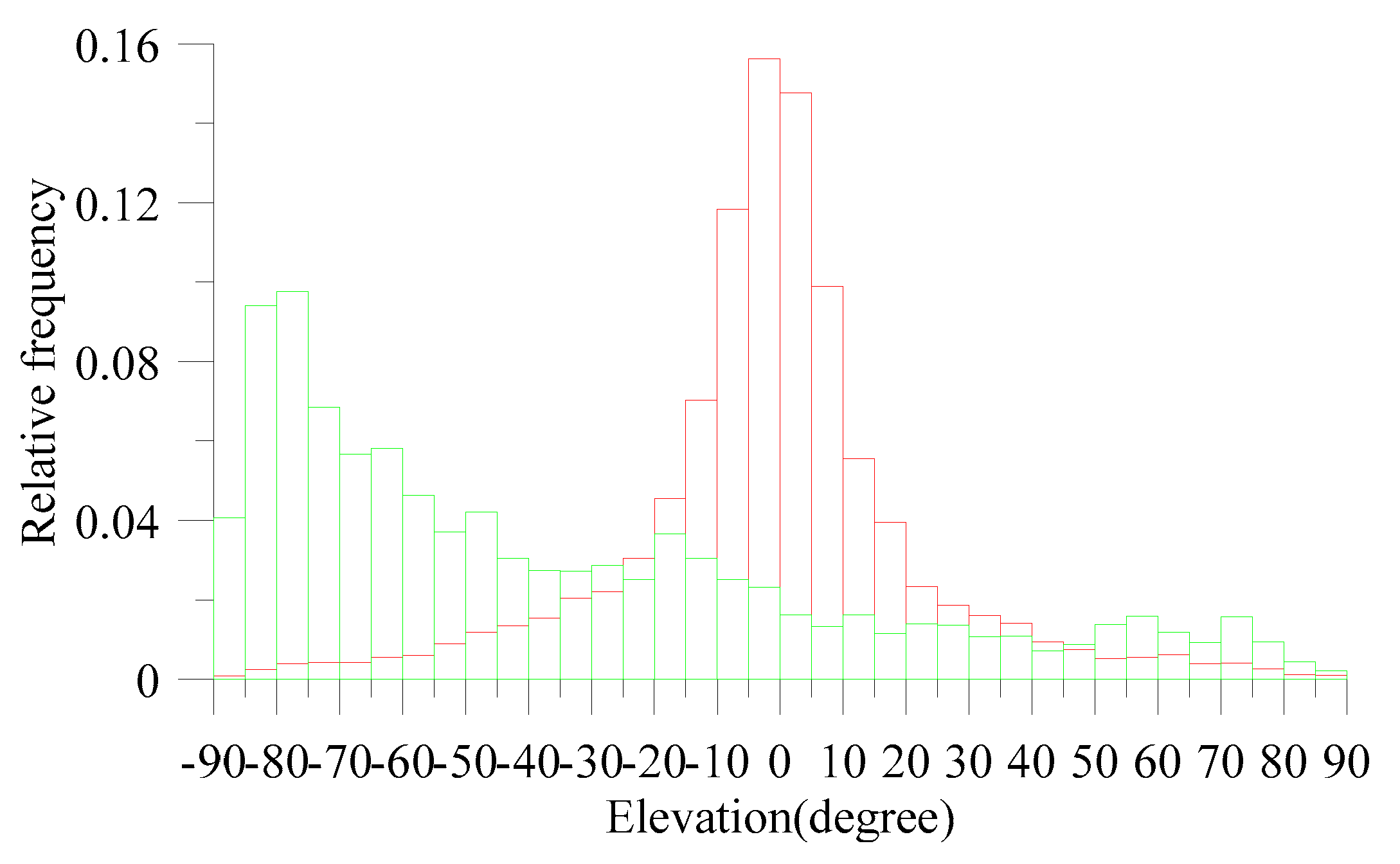
Thus, having the set of group velocities, we compared the elevation distributions for the $\overrightarrow{G}$ and $\overrightarrow{k}$ vectors (Figure 2).

On one hand, the difference between the most probable elevations of $\overrightarrow{G}$ and $\overrightarrow{k}$ should be close to 90°, as expected from Equation (5). On the other hand, the elevations of $\overrightarrow{k}$ should mainly be negative and the elevations of $\overrightarrow{G}$ would be expected to be mainly positive. Nevertheless, Figure 2 shows that elevations of $\overrightarrow{G}$ can be both negative and positive in about the same proportion. Equation (5) demonstrates that horizontal winds cannot change the elevation sign of $\overrightarrow{G}$, and only downward vertical winds can lead to the appearance of a large number of negative elevations. As will be shown in the Discussion section, vertical winds are generally mainly negative.

4. Method for Determining Neutral Wind Velocities

As mentioned above, using the dispersion relation, we can obtain the group velocity full vector in a coordinate system moving with a neutral wind velocity. From experimental data, we can detect the group velocity in a fixed coordinate system. Knowing the group velocity in a coordinate system moving with a neutral wind velocity and in a fixed coordinate system, we can calculate the neutral wind velocity full vector.

$$\{\begin{array}{l}{U}_x=G_x-G_x^{\prime }\\ U_y=G_y-G_y^{\prime }\\ U_z=G_z-G_z^{\prime }\end{array},$$

(9)

Here, G′ is the group velocity in a coordinate system moving with a neutral wind velocity (obtained from dispersion relation), while G is the group velocity in a fixed coordinate system (obtained from observations). Further, instead of the simple Boussinesq dispersion relation, we used the Hines [8] dispersion relation as it is the most precise one.

$$k^2=\frac{(k_x^2+k_y^2){\mathsf{\Omega }}_B{}^2}{{\omega \prime }^2}+\frac{{\omega \prime }^2-{\omega }_A^2}{C_0^2},$$

(10)

The group velocity (G′) is calculated by using the implicit-function derivative theory:

$$F({\omega }^{\prime },k_x,k_y,k_z)=\frac{(k_x^2+k_y^2){\mathsf{\Omega }}_B{}^2}{{\omega \prime }^2}+\frac{{\omega \prime }^2-{\omega }_A^2}{C_0^2},$$

(11)

$$\begin{array}{l}{G}_x^{\prime }=\frac{\partial {\omega }^{\prime }}{\partial k_x}=-\frac{\frac{\partial F}{\partial k_x}}{\frac{\partial F}{\partial {\omega }^{\prime }}}=\frac{k_x{\omega }^{\prime }{C}_0^2({\omega \prime }^2-{\mathsf{\Omega }}_B^2)}{({\omega \prime }^4-(k_x^2+k_y^2){\mathsf{\Omega }}_B^2{C}_0^2)}\\ G_y^{\prime }=\frac{\partial {\omega }^{\prime }}{\partial k_y}=-\frac{\frac{\partial F}{\partial k_y}}{\frac{\partial F}{\partial {\omega }^{\prime }}}=\frac{k_y{\omega }^{\prime }{C}_0^2({\omega \prime }^2-{\mathsf{\Omega }}_B^2)}{({\omega \prime }^4-(k_x^2+k_y^2){\mathsf{\Omega }}_B^2{C}_0^2)}\\ G_z^{\prime }=\frac{\partial {\omega }^{\prime }}{\partial k_z}=-\frac{\frac{\partial F}{\partial k_z}}{\frac{\partial F}{\partial {\omega }^{\prime }}}=\frac{k_z{C}_0^2{\omega \prime }^3}{({\omega \prime }^4-(k_x^2+k_y^2){\mathsf{\Omega }}_B^2{C}_0^2)}\end{array}$$

(12)

The intrinsic period (frequency) can be found from the Hines equation by solving a biquadratic equation:

$$\frac{{\cos }^2(\theta )}{T_b^2}{T\prime }^4-(1+\frac{L^2}{C_0^2{T}_A^2}){T\prime }^2+\frac{L^2}{C_0^2}=0,$$

(13)

where ω is the IGW frequency, k is the wave vector, Ω_B is the Brunt–Vaisala frequency (T_b is the Brunt–Vaisala period), θ is the wave front inclination angle, C₀ is the sound velocity, ω_A is the acoustic cutoff frequency (T_A is the acoustic cutoff period), and L is the wavelength. The environmental characteristics of the Hines dispersion relation (Brunt–Vaisala frequency, acoustic cutoff frequency, and sound velocity) were estimated from the MSIS2000 model [25]. Accordingly, from a dispersion relation, we are able to calculate the wind along the IGW propagation direction using Equation (2).

Therefore, Equation (9) should be added with equation:

$$\frac{k_x}{\left|k\right|}{U}_x+\frac{k_y}{\left|k\right|}{U}_y+\frac{k_z}{\left|k\right|}{U}_z=\frac{\omega -{\omega }^{\prime }}{\left|\overrightarrow{k}\right|},$$

(14)

In addition, when calculating group velocity in a fixed coordinate system, we assumed that the dispersion relation was valid at least three more frequencies (we called those ω₁, ω₂, ω₃); hence, Equation (9) should be added with three more equations, similar to Equation (14). Importantly, if the final system is found to be excessive, it can be solved using the mid-square method. It would seem that the neutral wind velocity full vector can be obtained from a single disturbance by solving a linear equation system. Moreover, taking into account the fact that a system may be excessive, we also can obtain other environmental characteristics. However, there are a number of problems:

(1)

Separation of TIDs due to their having a physical nature which differs from IGWs (Perkins instability, etc.).

(2)

We use simple dispersion relation (Hines) and assume simple Doppler frequency shift (Equation (1)) as a result of IGW interaction with a neutral wind. On one hand, we tested the Hines dispersion relation in our previous papers, wherein it was shown that the observational data were in good agreement with it [6,7]. There are other instances of Hines dispersion relation tests [17], and linear dispersion relations (for wind) have been used by other researchers [14,15,16,17,18]. Linearization is also used in modeling of IGWs [10,11,12,13]. On the other hand, we understand that there are many phenomena that do not obey the Hines dispersion relation and that it is therefore one potential source of error.

(3)

Method of TIDs detection. First of all, to detect TIDs, we assumed that dominant harmonics—with the highest energy concentration—could be isolated from the entire spectrum of a wave disturbance [5]. We also had to assume that the disturbance covered a certain frequency band and frequencies ω, ω₁, ω₂, ω₃ belonged to the same disturbance. Under the current method of disturbance detection, this condition cannot be guaranteed. Also, this method has a spectral problem. As the TID frequency is more precisely defined (and thus the elevation angle and wind velocity along the direction of TID propagation), the determination of TID time localization becomes less precise. Solving this problem requires developing new methods of TID detecting, which would need to combine spectral and non-spectral approaches.

The solution to all these problems is outside of the scope of this work, and in this study we tried to obtain only average wintertime diurnal wind variations. For wintertime, we had representative statistics (more than 5000 TIDs over the periods 16 January–16 February 2011, 17 January–9 February 2012, 25 December 2012–21 January 2013, and 26 December 2013–12 January 2014). We determined the neutral wind velocity at time t as the mean of all the wind velocities received by solving a linear equation system for IGWs observed in a time window [t − 2 h, t + 2 h], which corresponded to the following conditions:

(1)

For the four frequencies involved in group velocity detection, the maximum azimuthal difference could not exceed 60° (in this way, we tried to exclude cases where the group velocity was detected based on frequencies that did not belong to the same disturbance).

(2)

The wind velocity absolute value was less than 300 m/s (the maximum physically realistic neutral wind velocity at midlatitude ionospheric heights is ~300 m/s [21], and we tried to exclude nonlinear effects and TIDs not related to IGWs).

(3)

The angle between the group and phase velocities in the vertical plane was 60–120° (as a means to exclude TIDs not related to IGWs).

Having carried out calculations by the above scheme, we obtained diurnal wind variations.

5. Comparison and Discussion

We compared the neutral wind obtained from measurements of IGWs group and phase velocities with the HWM2007 model, results of our previously developed method [6,7], and FPI data. A radiophysical observations method was also used to obtain independent neutral wind data based on the observation of red airglow originating from a population of excited (1D state) oxygen atoms in the upper atmosphere. Previous research has indicated that the condition for generation of the most amount of red airglow is at an atmosphere height of about 250 km [26]. To get the neutral wind velocity, we needed to measure fine (~10⁻⁴ nm) shifts in the 630 nm atomic oxygen optical emission line, which occur as a result of the collective motion of oxygen atoms. Fabry–Perot interferometers are able to get neutral wind from a 630 nm line, and are widely used in modern aeronomy [27]. Therefore, such a device was used for additional observation of the neutral wind in the region where the IISR and ionosonde radars observed internal gravity waves. A detailed description of the device and method can be found in Ref. [22]. The method for determination of the neutral horizontal wind using this FPI was successfully tested and confirmed using a meteor radar also placed nearby [23]. Vertical wind velocity was also obtained by the FPI by reorientation of its entrance window. In this case, we needed to remove fake signals due to thermal variations of etalon size and systematic shifting which occurred as a consequence of the non-ideal etalon model. The first issue was solved by periodical (about every 10–15 min) calibration of the device by a stable reference laser light, as described in Ref. [22], while the second issue was fixed by averaging the dataset and removing the averaged value. We considered the variations that remained the variations of the vertical wind, and further discussion showed that this was apparently true. The FPI neutral wind velocities were averaged over the winters of 2016/2017, 2017/2018 and 2018/2019. Figure 3 shows the winter wind patterns obtained in various ways.

The horizontal wind diurnal variations obtained from the various methods were in qualitative agreement. Specifically, all showed eastward and southward winds in the nighttime, as well as westward and northward winds in the daytime. The zonal wind obtained by the new method was in greater agreement with the FPI results than the winds obtained by other methods. Qualitatively, the zonal wind obtained by the new method was in agreement with that of HWM2007, but there were significant quantitative differences. As the FPI and new method gave similar results, we considered that, in this case, the HWM2007 model did not describe the wind accurately. For the meridional wind, the new method noticeably underestimated the southward component given by the FPI. This disagreement may be explained by the following reasons: (1) Different periods of averaging and, accordingly, different periods of solar and geomagnetic activity; (2) influence of the problems described above; and (3) yet unknown systematic error that may be identified in the course of further testing. Thus, we consider that, in spite of the problems described above, our method allows for the obtainment of neutral wind from IGW characteristics. This result is important because: (1) It allows for the acquisition of neutral wind regardless of whether it is overcast, nighttime or daytime; (2) it may be useful for developing and testing wind models; (3) it shows the applicability of simple IGW dispersion relations; (4) it allows for testing of different IGW dispersion relations and theoretical concepts using the methodology proposed in this paper; and (5) it shows that the method is potentially capable of acquisition of “instant values” for neutral wind velocity full vector and other environmental characteristics.

Of particular interest were the results associated with the measurement of vertical wind velocities. The presence of large vertical wind velocities in the upper thermosphere causes controversy in the scientific community. Neither empirical nor physical models predict the presence of large vertical wind velocities. Large vertical velocities obtained with an FPI are sometimes interpreted as apparent vertical velocities due to horizontal wind and scattering in the upper troposphere [12]. Figure 3 shows that both the new method and FPI results possess the same diurnal trend in the vertical wind—about zero vertical velocity at midnight and an increase in downward velocity from midnight to dawn and from midnight to sunset. The largest value of the downward wind velocity (~20 m/s) is seen in the evening time. Thus, two absolutely independent methods indicated the presence of vertical wind velocities with an amplitude of ~20 m/s (this is the average velocity; the instantaneous values can be much higher).

Vertical winds with amplitudes of 10–20 m/s can have a significant effect on the wind-induced vertical drift of the ionospheric plasma. This effect may be comparable with the meridional wind effect. To clarify this issue, we calculated the contributions of the meridional (V_EFFX) and vertical (V_EFFZ) winds to the plasma drift velocity, as well as the total contribution, V_EFF, using:

$$V_{EFFX}=U_x\cos I\sin I,V_{EFFZ}=U_z{\sin }^{2}I,V_{EFF}=V_{EFFX}+V_{EFFZ},$$

(15)

where I is the magnetic field inclination (~72°). The calculated contributions were compared with the peak heights (hmF2) from the Irkutsk ionosonde averaged over the same period, and the correlation coefficients were calculated (Figure 4).

Figure 4 demonstrates that the contributions of the meridional and vertical winds to the plasma drift velocity are very close to each other, with the total contribution having the largest correlation coefficient with the height. These results clearly convey the importance of vertical wind measurements and the need to take them into account in physical and empirical models of the ionosphere and thermosphere.

6. Conclusions

The present study was performed on the basis of the analysis of 3-D characteristics of IGW propagation in the upper atmosphere of the Earth. Representative statistics of these characteristics were obtained using electron density profiles measured with the Irkutsk Incoherent Scatter Radar and DPS-4 ionosonde. An important component of the study is the automated method for determining the IGW characteristics, which allows for the processing of large amounts of data. The main result of this study is the development of a new method for determining neutral wind velocity vectors, based on IGW group velocity measurements. In contrast to previously developed methods [6,7], the new method allows us to obtain not only a statistical pattern, but also potentially instantaneous values of the neutral wind velocity. Another advantage of the new method is the ability to measure the vertical velocity of the neutral wind.

Testing of the new method showed that it was in quantitative agreement with the FPI wind measurements for zonal and vertical wind velocities. The difference observed in meridional wind velocities may be related to different periods of averaging, the simplicity of the dispersion relation used, or a possible systematic error. The quantitative agreement between the new method and the FPI data is important because: (1) It allows for the acquisition of neutral wind regardless of whether it is overcast, nighttime or daytime; (2) it may be useful for developing and testing wind models; (3) it shows the applicability of simple IGW dispersion relations; (4) it allows for testing of different IGW dispersion relations and theoretical concepts using the methodology proposed in this paper; and (5) it shows that the method potentially allows for acquisition of “instant values” for neutral wind velocity full vector and other environmental characteristics.

Of particular interest were the results associated with the measurement of vertical wind velocities. We demonstrated that two absolutely independent methods gave the presence of vertical wind velocities with an amplitude of ~20 m/s. Estimation of the vertical wind contribution to the plasma drift velocity indicated the importance of vertical wind measurements and the need to take them into account in physical and empirical models of the ionosphere and thermosphere.