How Can the International Monitoring System Infrasound Network Contribute to Gravity Wave Measurements?

Abstract

Gravity waves (GWs) propagate horizontally and vertically in the atmosphere. They transport energy and momentum, and therefore GWs can affect the atmospheric circulation at different altitude layers when dissipating. Thus knowledge about the occurrence of GWs is essential for Numerical Weather Prediction (NWP). However, uniform networks for covering GW measurements globally are rare, especially in the troposphere. It has been shown that an infrasound station of the International Monitoring System (IMS) infrasound network is capable of measuring GWs at the Earth’s surface. The IMS was deployed for monitoring the atmosphere to verify compliance with the Comprehensive Nuclear-Test-Ban-Treaty. In this study, the Progressive Multi-Channel Correlation Method (PMCC) is used for re-processing up to 20 years of IMS infrasound recordings in order to derive GW detections. For this purpose, two alternative PMCC configurations are discussed, covering GW frequencies equivalent to periods of between 5 min and 150 min. These detections mainly reflect sources of deep convection, particularly in the tropics. At mid-latitudes, coherent wind noise more often produces spurious detections. Combining the results of both configurations provides a global dataset of ground-based GW measurements, which enables the calculation of GW parameters. These can be used for improving NWP models.

1. Introduction

Gravity waves (GWs) play a critical role in atmospheric dynamics as they transport energy and momentum [1]. Due to the exponential density decrease with altitude, the amplitude of a vertically-propagating wave increases. Consequently, its impact in the middle atmosphere, which comprises of the stratosphere (approximately 12–50 km) and mesosphere (50–90 km), is more significant than in the troposphere (<12 km). A breaking GW deposits its momentum to the mean flow, resulting in an alteration of the latter [2,3]. There is evidence that such modification of the middle-atmosphere dynamics impacts the tropospheric circulation [4].

Therefore, knowledge about GW sources and their magnitude is essential for numerical weather modeling [5]. However, methods for measuring GW parameters, such as the momentum flux, are rare [6], especially in the middle atmosphere [7]. On the other hand, global estimates of GW activity are often the preserve of satellite observations probing the middle atmosphere [8,9,10,11]. Ground-based observation methods—such as light detection and ranging (lidar)—provide high-resolution vertical measurements which are used to extract GW parameters at different altitudes [12], but such technologies lack temporal coverage and global distribution.

It has recently been shown that highly-sensitive infrasound sensors are additional instruments that are suitable for measuring GW activity at the surface [13,14,15,16]. Infrasound is one of the International Monitoring System (IMS) technologies that are dedicated to verifying compliance with the Comprehensive Nuclear-Test-Ban Treaty (CTBT). Sixty globally-distributed infrasound stations are planned to be part of the IMS. Out of these, currently, 51 stations (Figure 1) almost continuously measure atmospheric pressure disturbances of from 10⁻³ to 10 Pa.

These recordings of a particular IMS infrasound station, IS17 in Côte d’Ivoire, were used by [16] for deriving GW parameters—more precisely, they argued that only trapped GWs cause traceable pressure fluctuations at the surface. Before that study, [13] reported on infrasound-based GW observations at the same station. They used the Progressive Multi-Channel Correlation (PMCC) method [17,18] for the automatic detection of such events. The back-azimuth of the detections showed a clear correlation with the seasonal movement of the Inter-Tropical Convergence Zone (ITCZ) relative to the station. For the calculation of GW parameters, such as horizontal and vertical wavenumber, the authors of [16] combined the PMCC detection parameters and meteorological data. This allowed estimating the vertical GW momentum flux at the top of the ducting layer, which was shown for a particular event detected at IS17.

In this study, we discuss two different adaptions of the PMCC configuration for automatically detecting GWs and acoustic-GWs at infrasound stations worldwide. Based on the two proposed configurations (Section 2), the complete IMS infrasound dataset has been re-processed. Combining both processing results, which are provided in Section 3, makes a unique global dataset. It will enable the determination of GW parameters, the calculation of which was described in detail by [16]. These GW parameters will be a valuable supplement to existing global GW climatologies since they build upon ground-based measurements with a high temporal resolution. Therefore, in addition, these data can be made available in near-real time, and are of interest for civil applications such as numerical weather modelling and prediction. Specific features, and limitations of the processing—e.g., concerning detection capabilities and an adjustment towards long-period scales—are discussed in Section 4. Conclusions are drawn in Section 5.

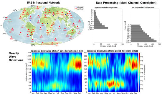
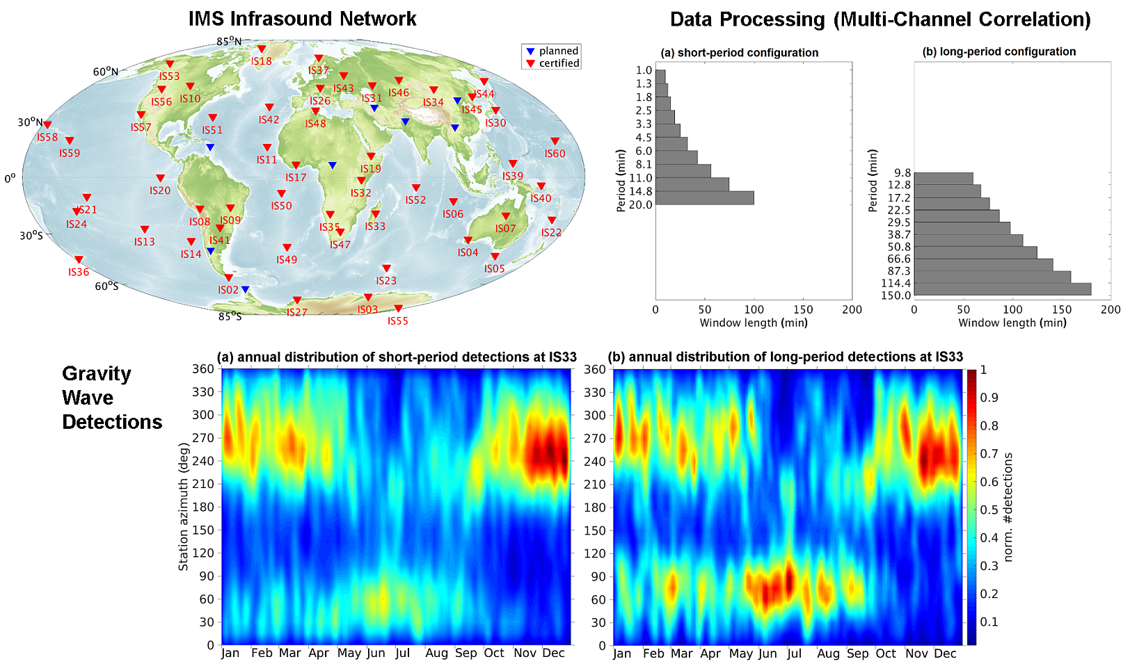
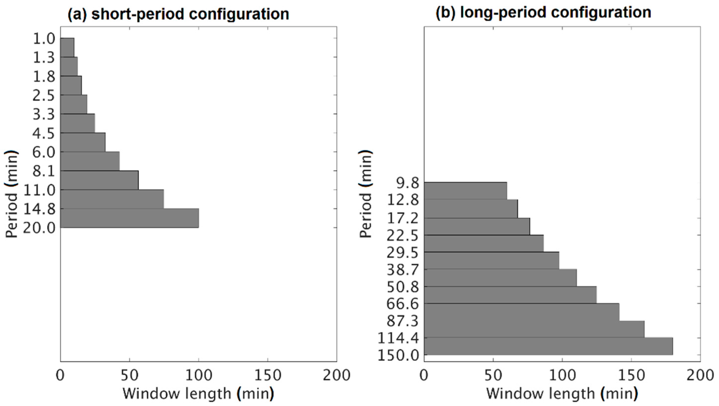
2. Processing

Each IMS infrasound station consists of at least four microbarometers which form an array. The average array aperture is between 1 km and 3 km [19]. Each array element features a wind noise reduction system, which composes of various pipe structures connecting the inlet ports to a summing chamber. This design is supposed to filter out a large number of local wind fluctuations, including turbulent noise of higher frequencies. The PMCC algorithm has commonly been used to distinguish coherent signals from remaining noise in infrasound recordings [18,20]. The time delays between the sensors allow estimating the apparent phase velocity and direction of a passing wave, assuming it is a plane wave in the x-y-domain. Time delays are calculated by correlating the signals between the sensors.

PMCC performs cross-correlation tests in predefined frequency bands. After applying band-pass filters to the differential pressure time series, the signal is cut into time windows [17]. Cross-correlation is performed between the outputs from the different sensors, and if, for a given time and frequency, the delay times are consistent with a propagating wave front, a detection is declared—a ‘pixel’ in the time-frequency space. Each detected pixel is attributed a frequency, time, amplitude, back-azimuth, and apparent velocity. Pixels exhibiting similar wave front parameters within an evaluated time–frequency domain are clustered into families [21]; hence, the family size is a measure of the dominance of an event. The event lists contain the aforementioned wave front parameters averaged over all pixels of a family. A standard deviation is given for the back-azimuth and the apparent phase velocity; PMCC also provides the coherency and mean correlation coefficient. Those arrivals that cannot be associated with the dominant family in a given time window and frequency band are disregarded [17].

The predefined frequency bands for infrasound data commonly range from 0.01 to 5 Hz. The highest frequency of GWs is the Brunt–Väisälä frequency, which depends on temperature, humidity, and thus altitude and varies between around 10⁻² Hz and 3 × 10⁻³ Hz. The acoustic cut-off frequency varies accordingly. The long-period spectrum, representing the GW and acoustic–GW domains, is neglected by the common PMCC configuration. Therefore the frequency bands were adjusted for this study. One of the two configurations being discussed emphasizes very low periods, down to 1 min; the upper period limit is 20 min. The second configuration covers a broader period scale, ranging from 15 min to 150 min. The logarithmically-spaced frequency bands and the corresponding window lengths are shown in Figure 2.

Using the PMCC version 4.4 and the configurations given in Figure 2, the entire infrasound data set—i.e., differential pressure—was re-processed. For each detection family, the Fisher ratio (F) was additionally obtained, using the F-detector [22,23]. The F-detector compares the variance of background noise plus the coherent signal with the variance of noise only; hence, F equals one for uncorrelated noise; whereas F exceeds one if a coherent signal is recorded. The following equation relates F to the signal-to-noise ratio (SNR), according to [23]:

$$\mathrm{F}={\mathrm{N}}_{\mathrm{array}}\times {\mathrm{SNR}}^2+1$$

(1)

where N_array is the number of array elements contributing to the analysis. Equation (1) allows the use of F for filtering the detections concerning significance. The authors of [24] statistically tested that a recorded signal will contain a coherent signal when F > 3 with a confidence level of 99%. This threshold was therefore applied to filter the PMCC detections. Remaining infrasonic signals were also filtered out; more precisely, the upper limit of the apparent phase velocity was set to 50 m s⁻¹. A global overview of the monthly predominant detections at each station, and examples of the seasonal variation in detections at particular stations are presented in the following section.

For classifying the results and characterizing potential sources of the detected GWs, the high-resolution monthly climatology (HRMC) lightning data set of [25] was considered since it is assumed that regions of enhanced lightning activity go along with deep convection, which is among the sources of atmospheric GWs [1,26]. The HRMC provides the mean flash rate per square kilometer and day in the middle of each month [27]. It incorporates data from two satellite-based detectors—the Optical Transient Detector and the Lightning Imaging Sensor.

3. Results

For the two processing results, global overviews of the detections, and detailed analyses of particular stations—IS33 and IS02—are shown.

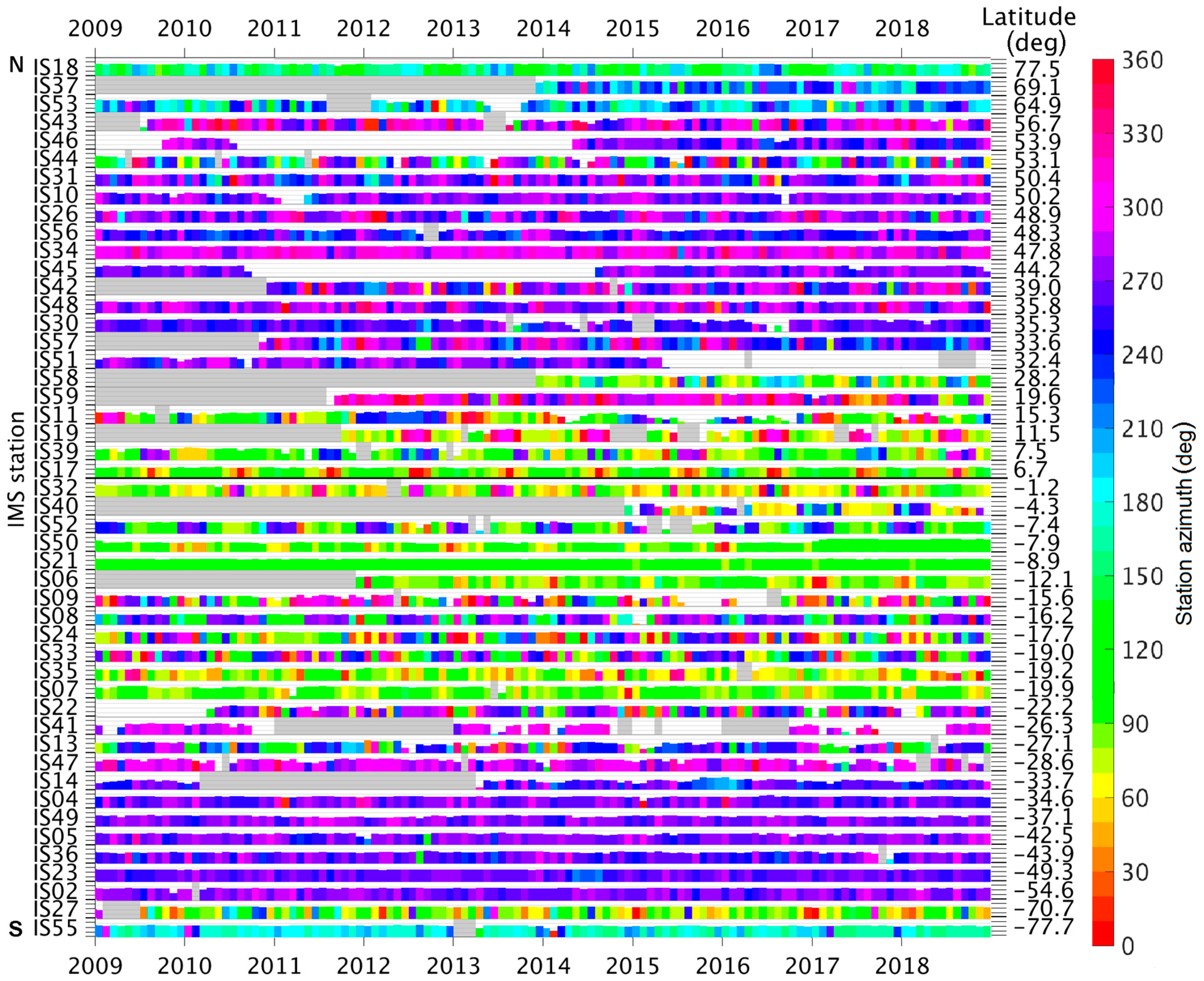
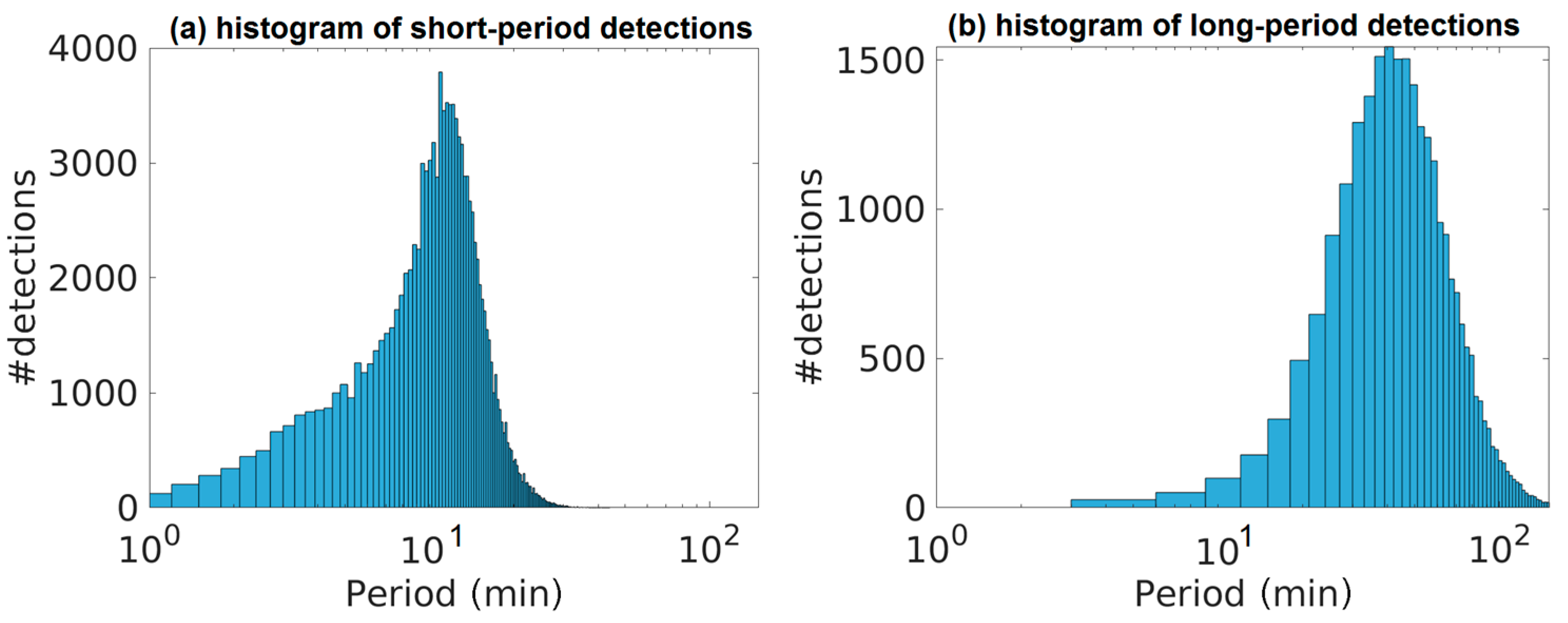
3.1. A Global Dataset of Gravity Wave Detections

Figure 3 shows a comprehensive overview of the long-period GW detections at 48 certified IMS infrasound stations for the last 10 years—in particular, the mean back-azimuth (color-coded) and the number of detections (vertical scale) per month. The analogous overview of the short-period configuration is given in the Appendix A (Figure A1). This mainly differs from Figure 3 in the number of detections (three to four times), rather than the azimuthal variation.

At first glance, the majority of the detections are attributed to back-azimuths which represent the predominant tropospheric wind directions. At mid-latitudes, westerly directions (bluish and purple colors) prevail; whereas in the tropics and at high latitudes, the majority of the detections originate from easterly directions (greenish and yellow). However, a seasonal variation can be recognized at many stations, especially in the tropical latitudes.

At IS17, for instance, arrivals from the north are characteristic in the Northern Hemisphere summer; whereas eastern directions prevail in the remaining of the year. As reported in [13], this seasonal variation is associated with the ITCZ. Figure 3 indicates similar seasonal variabilities at a couple of further stations, of which IS32 (Kenya) and IS33 (Madagascar) are analyzed in more detail below (Section 3.2). In addition, the mid-latitude station detections of IS02 (Argentina) are focused on (Section 3.3).

It is noted that IS21 on the Marquesas Islands in the Pacific Ocean exhibits only slightly varying back-azimuths between easterly and southeasterly directions; whereas at the closest station, IS24 (Tahiti), the back-azimuths significantly vary throughout a year, covering almost all conceivable directions. This discrepancy can result from the different array configurations. IS21 is a four-sensor array, with three microbarometers surrounding a central one. The horizontal dimension is around 2 × 2 km. The aperture of IS24 is larger (around 3.5 × 2.2 km), with a total of five sensors, and is presumably more sensitive to the relevant spatial scales of GWs. The array response, in general, is discussed in Section 4.

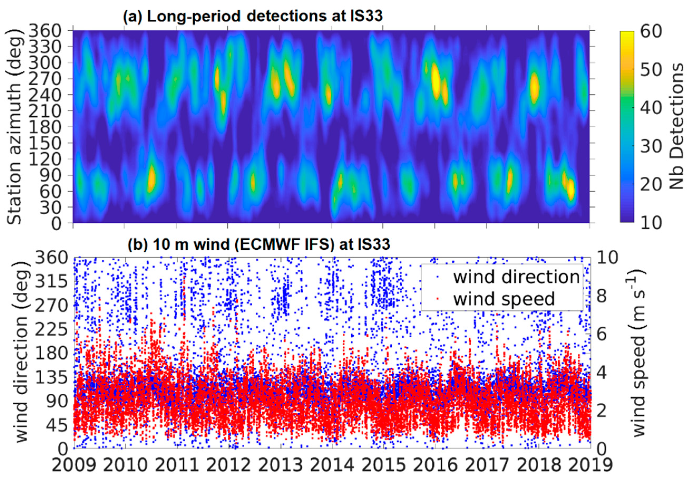
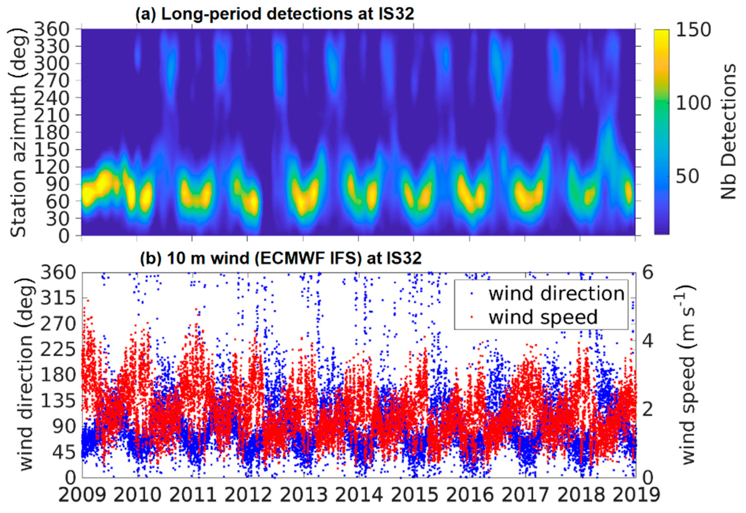
3.2. Gravity Wave Detections at Tropical Stations

The infrasound station IS33 provides continuous recordings within the last 10 years, resulting in 113,046 short-period and 28,155 long-period detections. The histograms with regard to the ground-based period are shown in Figure 4. The periods at which the histograms peak—13 min and 60 min, respectively—are beyond the acoustic–GW range, so the majority of detections can be assumed to be internal GWs. Note that the intrinsic wave period can be obtained by incorporating the along-path wind. The calculation was demonstrated in [16].

Figure 5 compares the seasonal variations in detections and azimuth resulting from the two configurations at IS33. The detections are stacked over 10 years and normalized by the maximum number within this distribution. During austral summer, the majority of GW signals are detected from westerly directions. Since IS33 is located in the northeast of Madagascar, these signals can originate from the vicinity of the station, or from the mainland of the African continent. The heating of the land surfaces in the summer induces deep convection that results in increased thunderstorm activity, as indicated by the lightning maps (e.g., January) given in the Appendix A (Figure A2). In the winter, detections from northeastern directions likely represent deep convection over the Indian Ocean. For the short-period configuration, the number of detections in the winter is lower than in the summer; whereas for the long-period configuration, the maximum numbers of detections in the winter and summer, from easterly and westerly directions, respectively, equalize (Figure 5b).

This finding allows the conclusion that the GW activity is enhanced over the land masses, compared with the oceans. The difference in the number of detections from both directions at short periods could be indicative of different excitation mechanisms being captured; for instance, the rapid development of convective cells will induce GWs that differ from GWs that result from the flow over convective cells. It was stated in [1] that deep convection is complex in terms of the variety of phase velocities and intrinsic frequencies.

The variation in detections and azimuth is compared to the 10 m wind at the stations, with regard to the impression of Figure 3, according to which the monthly-mean back-azimuths of the detections followed the prevailing tropospheric wind directions. Figure 6 compares the time series of detections with the wind direction (blue) and wind speed (red) at IS33. Obviously, the detections’ azimuths correlate with the wind direction, especially detections originating from the west. At the same time, the wind speeds are at the annual minimum (around 1–2 m s⁻¹); contrarily, detections from the east coincide with higher seasonal wind speeds (around 3–4 m s⁻¹). In the winter, the stronger winds blowing from the ocean reduce the detection capability of the station since these cause more turbulent noise. The detection capability can also be an explanation for the reduced number of detections from the east, specifically at short periods.

Another infrasound station that shows an evident variation in the detections is IS32, which is directly located at the Equator. The direction of the arrivals (Figure 7) shifts from the east in October to the northeast in December, and back to the east until March. This variation is again well correlated with the wind direction near the surface, but also coincides with wind speeds of 2 to 4 m s⁻¹. In June and July, detections from the northwest prevail during weak wind conditions (1 m s⁻¹) from the south. It is also noted that the preferred direction of the detections in June and July agrees with maximum lightning activity from the northwest (Appendix A, Figure A2c). However, in December and January, the lightning maps (Appendix A, Figure A2a) would imply detections from the southwest, rather than from the northeast. Since trapped GWs can sometimes be horizontally-propagating waves [28], these either perturb the background flow or are embedded within, which is likely the case for IS32 detections in December and January.

3.3. Gravity Wave Detections near a Mid-Latitude Hotspot of Orographic GWs

Here, the detections of IS02 in southern Argentina are analyzed. These comprise 101,100 short-period and 42,828 long-period detections. The station is located in the lee of the southern Andes hotspot for orographic GWs [29,30]. The predominant direction of signals is from the west (Figure 8), which corresponds with the prevailing wind direction in the lower troposphere and near the surface (Figure 9). The relatively high cross-mountain wind speeds of around 5 m s⁻¹ favor the excitation of GWs throughout the whole year, the majority of which propagate vertically into the middle atmosphere. However, strong GW momentum fluxes in the stratosphere have only been found in the winter season [26,30]. In the summer, the critical level causes upward-propagating GWs to break at lower altitudes due to dynamic instabilities [31,32,33].

Figure 8 shows the most GW detections during the austral summer when the wind speeds at the station (at 10 m) are higher (>5 m s⁻¹) than in the winter (<4 m s⁻¹). This can be an indication that trapped lee waves are detected downstream; whereas the reduced number of detections in the winter underlines that the infrasound arrays are not capable of recording stationary, upward-propagating GWs.

4. Discussion

At first sight, and for both proposed configurations, the back-azimuths of detections at mid-latitude stations reflect the prevailing westerly wind directions. The seasonal variation at IS02 implies that the detections represent horizontally-propagating lee waves downstream of the southern Andes. However, the variation of several mid-latitude stations is similar in terms of the azimuth and the number of detections, although mountain ranges are not necessarily in the vicinity of such stations (e.g., IS04 in Western Australia). A possible explanation, with regard to orographic waves, is that horizontally-propagating waves have been modeled over distances of hundreds to thousands of kilometers [34,35]. However, coherent noise due to relatively strong tropospheric winds in the mid-latitudes, compared with tropical latitudes, may be considered as another source of the detections.

The authors of [36], who used an array of four microbarographs in Southern Germany similar to the IMS stations, stated the difficulties of attributing the different pressure signatures a specific source process. Besides GWs, they identified signatures from coherent, drifting density patterns; solitary waves; fronts; and uncorrelated fluctuations due to turbulence. The latter phenomenon is assumed to be not relevant here, following from the array design and processing method (Section 2). However, coherent, drifting density structures can lead to overestimating the presence of GWs [36]. This is especially relevant at mid-latitudes (e.g., IS02) and needs to be further investigated, which is beyond the scope of this study.

The detections of the long-period PMCC configuration, which allows periods up to 150 min, show a bias towards periods of around 60 min, with only a few detections remaining between 60 min and 150 min. It is assumed that the apertures of the infrasound arrays (1–3 km) limit the GW detectability in terms of the wavelength, implying that longer wavelengths and larger-period scales are technically omitted. Figure 10 shows normalized array responses as a function of horizontal wave numbers. Since the wavelengths of GWs are in the range of a few to hundreds of kilometers [33]—i.e., the wave numbers are fractions of one—the discrimination of detections in the chosen frequency ranges is challenging, especially at IS02. Consequently, the next re-processing of the entire data set for detecting GWs should only consider specific sensors of the arrays.

Also, the infrasound sensors are primarily supposed to detect acoustic signals; hence, differential pressure fluctuations induced by waves below a frequency of 10⁻² Hz are suppressed. This affects the capability of the PMCC to discriminate these waves from noise. For this reason, the need for station-specific amplitude corrections was proposed in [16].

Besides orographic GWs, the potential sources of detected GWs include jet-stream instabilities, polar fronts, geostrophic adjustment, and deep convection [1,37]. GWs caused by jet-stream instabilities would also agree with the correlation between detections and tropospheric winds. Such sources can release downward-propagating GWs, which will induce pressure fluctuations at the surface. In general, GWs induced by deep convection in tropical latitudes are characterized by short horizontal wavelengths [26] and various non-zero phase velocities [1]. As a result, the PMCC GW detections at tropical stations, such as IS17 and IS33, where the noise level is lower, well represent GWs related to deep convection of the ITCZ. However, in addition to the ITCZ, the prevailing tropospheric wind direction needs to be considered for understanding the seasonal variation in back-azimuth. Although the deep convection is presumably more intense over the continents, as shown using the lightning climatology of [25], deep convection originating over the oceans has also been detected.

A valuable application would be to use the IMS infrasound network for the localization of GW sources, based on detections by the PMCC algorithm. Comparable cross-bearing approaches have been carried out for infrasound phenomena such as microbaroms [20,38] and mountain-associated infrasound waves [39]. Due to the relation of the detected GWs to tropospheric winds, and the low phase velocities (i.e., 10% of the sound speed), it is unlikely that the IMS infrasound stations detect the same GW sources—the average distance between the stations is 2000 km [40]. Consequently, a cross-bearing approach is not promising.

5. Conclusions

Two configurations for detecting GWs using the PMCC algorithm were proposed. The monthly re-processing results of the global IMS infrasound network showed seasonal variations in the direction of origin, associated with deep convection and predominant tropospheric wind directions. For the majority of tropical IMS infrasound stations, it is concluded that GWs from convective sources are the dominant signatures since the detections follow an azimuthal variation related to deep convection. However, this study also exhibited the limitations of the processing in terms of detecting stationary GWs or GWs with periods beyond 120 min. The latter issue could be addressed in the future by carefully selecting specific sub-networks of the IMS arrays in order to maximize the array aperture. This may clarify whether the detections at mid-latitude stations originate from lee waves propagating near the surface, implying long-distance propagation, or from coherent noise such as drifting density fluctuations.

In this context, and also for detecting GWs of a larger scale, infrasound sensors within denser regional networks, such as the low-frequency array (LOFAR) in the Netherlands [41], are promising because these sensors can be combined to obtain larger apertures of tens to hundreds of kilometers. For instance, the detection of GWs with periods of 120 min to 360 min has been demonstrated within the dense USArray Transportable Array infrasound network [15], consisting of around 400 barometric sensors separated by 70 km [42]. A future intention is to equip the existing infrastructure of the Gräfenberg Array in Germany with infrasound sensors. The seismological array has an aperture of around 50 km (east–west) times 100 km (north–south) and comprises of 13 sites [43].

Nevertheless, the IMS infrasound network will play a key role since it is the only homogeneously, world-wide distributed array network which enables GW studies at all latitudes, providing data for up to 20 years. Since it has been shown that specific GW parameters, including the momentum flux, can be calculated from the PMCC detections [16], the re-processed IMS data set is worth supplementing existing GW parameter climatologies. The IMS infrasound network could thus contribute to improving the representation and parameterization of GWs in numerical weather prediction models.

References

- Fritts, D.C.; Alexander, M.J. Gravity wave dynamics and effects in the middle atmosphere. Rev. Geophys. 2003, 41, 1003. [Google Scholar] [CrossRef]
- Holton, J.R. The Influence of Gravity Wave Breaking on the General Circulation of the Middle Atmosphere. J. Atmos. Sci. 1983, 40, 2497–2507. [Google Scholar] [CrossRef]
- Gill, A.E. Atmosphere-Ocean Dynamics, 1st ed.; Academic Press: San Diego, CA, USA, 1982. [Google Scholar]
- Baldwin, M.P.; Dunkerton, P.J. Stratospheric Harbingers of Anomalous Weather Regimes. Science 2001, 294, 581–584. [Google Scholar] [CrossRef] [PubMed]
- Charlton-Perez, A.J.; Baldwin, M.P.; Birner, T.; Black, R.X.; Butler, A.H.; Calvo, N.; Davis, N.A.; Gerber, E.P.; Gillett, N.; Hardiman, S.; et al. On the lack of stratospheric dynamical variability in low-top versions of the CMIP5 models. J. Geophys. Res. 2013, 118, 2494–2505. [Google Scholar] [CrossRef]
- Geller, M.A.; Alexander, M.J.; Love, P.T.; Bacmeister, J.; Ern, M.; Hertzog, A.; Manzini, E.; Preusse, P.; Sato, K.; Scaife, A.A.; et al. Comparison between gravity wave momentum fluxes in observations and climate models. J. Clim. 2013, 26, 6383–6405. [Google Scholar] [CrossRef]
- Baumgarten, G. Doppler Rayleigh/Mie/Raman lidar for wind and temperature measurements in the middle atmosphere up to 80 km. Atmos. Meas. Tech. 2010, 3, 1509–1518. [Google Scholar] [CrossRef]
- Ern, M.; Trinh, Q.T.; Preusse, P.; Gille, J.C.; Mlynczak, M.G.; Russell, J.M., III; Riese, M. GRACILE: A comprehensive climatology of atmospheric gravity wave parameters based on satellite limb soundings. Earth Syst. Sci. Data 2018, 10, 857–892. [Google Scholar] [CrossRef]
- Hoffmann, L.; Xue, X.; Alexander, M.J. A global view of stratospheric gravity wave hotspots located with Atmospheric Infrared Sounder observations. J. Geophys. Res. 2013, 118, 416–434. [Google Scholar] [CrossRef]
- Preusse, P.; Eckermann, S.D.; Ern, M. Transparency of the atmosphere to short horizontal wavelength gravity waves. J. Geophys. Res. 2008, 113, D24104. [Google Scholar] [CrossRef]
- Rapp, M.; Dörnbrack, A.; Kaifler, B. An intercomparison of stratospheric gravity wave potential energy densities from METOP GPS radio occultation measurements and ECMWF model data. Atmos. Meas. Tech. 2018, 11, 1031–1048. [Google Scholar] [CrossRef]
- Ehard, B.; Kaifler, B.; Kaifler, N.; Rapp, M. Evaluation of methods for gravity wave extraction from middle-atmospheric lidar temperature measurements. Atmos. Meas. Tech. 2015, 8, 4645–4655. [Google Scholar] [CrossRef]
- Blanc, E.; Farges, T.; Le Pichon, A.; Heinrich, P. Ten year observations of gravity waves from thunderstorms in Western Africa. J. Geophys. Res. Atmos. 2014, 119, 6409–6418. [Google Scholar] [CrossRef]
- Marty, J.; Ponceau, D.; Dalaudier, F. Using the International Monitoring System infrasound network to study gravity waves. Geophys. Res. Lett. 2010, 37, L19802. [Google Scholar] [CrossRef]
- De Groot-Hedlin, C.D.; Hedlin, M.A.H.; Hoffmann, L.; Alexander, M.J.; Stephan, C.C. Relationships between gravity waves observed at earth’s surface and in the stratosphere over the Central and Eastern United States. J. Geophys. Res. Atmos. 2017, 122, 11482–11498. [Google Scholar] [CrossRef]
- Marlton, G.; Charlton-Perez, A.; Harrison, R.G.; Lee, C. Calculating Atmospheric Gravity Wave Parameters from Infrasound Measurements. In Infrasound Monitoring for Atmospheric Studies—Challenges in Middle-atmosphere Dynamics and Societal Benefits, 2nd ed.; Le Pichon, A., Blanc, E., Hauchecorne, A., Eds.; Springer: Dordrecht, The Netherlands, 2019; pp. 701–718. ISBN 978-3-319-75138-2. [Google Scholar] [CrossRef]
- Cansi, Y. An automatic seismic event processing for detection and location: The P.M.C.C. Method. Geophys. Res. Lett. 1995, 22, 1021–1024. [Google Scholar] [CrossRef]
- Le Pichon, A.; Matoza, R.; Brachet, N.; Cansi, Y. Recent Enhancements of the PMCC Infrasound Signal Detector. Inframatics 2010, 26, 5–8. [Google Scholar]
- Christie, D.R.; Campus, P. The IMS Infrasound Network: Design and Establishment of Infrasound Stations. In Infrasound Monitoring for Atmospheric Studies; Le Pichon, A., Blanc, E., Hauchecorne, A., Eds.; Springer: Dordrecht, The Netherlands, 2010; pp. 29–75. ISBN 978-1-4020-9508-5. [Google Scholar] [CrossRef]
- Ceranna, L.; Matoza, R.S.; Hupe, P.; Le Pichon, A.; Landès, M. Systematic Array Processing of a Decade of Global IMS Infrasound Data. In Infrasound Monitoring for Atmospheric Studies—Challenges in Middle-atmosphere Dynamics and Societal Benefits, 2nd ed.; Le Pichon, A., Blanc, E., Hauchecorne, A., Eds.; Springer: Dordrecht, The Netherlands, 2019; pp. 471–482. ISBN 978-3-319-75138-2. [Google Scholar] [CrossRef]
- Brachet, N.; Brown, D.; Le Bras, R.; Cansi, Y.; Mialle, P.; Coyne, J. Monitoring the Earth’s Atmosphere with the Global IMS Infrasound Network. In Infrasound Monitoring for Atmospheric Studies; Le Pichon, A., Blanc, E., Hauchecorne, A., Eds.; Springer: Dordrecht, The Netherlands, 2010; pp. 77–118. ISBN 978-1-4020-9508-5. [Google Scholar] [CrossRef]
- Fisher, R.A. Statistical Methods for Research Workers. In Breakthroughs in Statistics: Methodology and Distribution; Kotz, S., Johnson, N.L., Eds.; Springer: New York, NY, USA, 1992; pp. 66–70. ISBN 978-1-4612-4380-9. [Google Scholar] [CrossRef]
- Melton, B.S.; Bailey, L.F. Multiple signal correlators. Geophysics 1957, 22, 565–588. [Google Scholar] [CrossRef]
- Olson, J.V. Infrasound signal detection using the Fisher F-statistics. Inframatics 2004, 6, 1–8. [Google Scholar]
- Cecil, D.J. LIS/OTD Gridded Lightning Climatology Data Collection; Version 2.3.2015 [0.5 Degree High Resolution Monthly Climatology (HRMC)], Data Set; NASA EOSDIS Global Hydrology Resource Center Distributed Active Archive Center: Huntsville, AL, USA, 2015. [Google Scholar] [CrossRef]
- Ern, M.; Preusse, P.; Gille, J.C.; Hepplewhite, C.L.; Mlynczak, M.G.; Russell, J.M.; Riese, M. Implications for atmospheric dynamics derived from global observations of gravity wave momentum flux in stratosphere and mesosphere. J. Geophys. Res. Atmos. 2011, 116, D19107. [Google Scholar] [CrossRef]
- Cecil, D.J.; Buechler, D.E.; Blakeslee, R.J. Gridded lightning climatology from TRMM-LIS and OTD: Dataset description. Atmos. Res. 2014, 135–136, 404–414. [Google Scholar] [CrossRef]
- Worthington, R.M.; Thomas, L. The frequency spectrum of mountain waves. Q. J. R. Meteorol. Soc. 1998, 124, 687–703. [Google Scholar] [CrossRef]
- De la Torre, A.; Alexander, P.; Hierro, R.; Llamedo, P.; Rolla, A.; Schmidt, T.; Wickert, J. Large-amplitude gravity waves above the southern Andes, the Drake Passage, and the Antarctic Peninsula. J. Geophys. Res. 2012, 117, D02106. [Google Scholar] [CrossRef]
- Hoffmann, L.; Grimsdell, A.W.; Alexander, M.J. Stratospheric gravity waves at Southern Hemisphere orographic hotspots: 2003–2014 AIRS/Aqua observations. Atmos. Chem. Phys. 2016, 16, 9381–9397. [Google Scholar] [CrossRef]
- Alexander, P.; Luna, D.; Llamedo, P.; de la Torre, A. A gravity waves study close to the Andes mountains in Patagonia and Antarctica with GPS radio occultation observations. Ann. Geophys. 2010, 28, 587–595. [Google Scholar] [CrossRef]
- Dörnbrack, A.; Gerz, T.; Schumann, U. Turbulent breaking of overturning gravity waves below a critical level. Appl. Sci. Res. 1995, 54, 163–176. [Google Scholar] [CrossRef]
- Nappo, C.J. An Introduction to Atmospheric Gravity Waves, Vol. 102 of International Geophysics; Academic Press: San Diego, CA, USA, 2012; ISBN 978-0-12-385223-6. [Google Scholar] [CrossRef]
- Sato, K.; Tateno, S.; Watanabe, S.; Kawatani, Y. Gravity wave characteristics in the Southern Hemisphere revealed by a high-resolution middle-atmospheric general circulation model. J. Atmos. Sci. 2012, 69, 1378–1396. [Google Scholar] [CrossRef]
- Jiang, Q.; Doyle, J.; Reinecke, A. A modeling study of stratospheric waves over the southern Andes and Drake Passage. J. Atmos. Sci. 2013, 70, 1668–1689. [Google Scholar] [CrossRef]
- Hauf, T.; Finke, U.; Neisser, J.; Bull, G.; Stangenberg, J.G. A Ground-Based Network for Atmospheric Pressure Fluctuations. J. Atmos. Oceanic Technol. 1996, 13, 1001–1023. [Google Scholar] [CrossRef]
- Plougonven, R.; Zhang, F. Internal gravity waves from atmospheric jets and fronts. Rev. Geophys. 2014, 52, 33–76. [Google Scholar] [CrossRef]
- Landès, M.; Ceranna, L.; Le Pichon, A.; Matoza, R.S. Localization of microbarom sources using the IMS infrasound network. J. Geophys. Res. 2012, 117, D06102. [Google Scholar] [CrossRef]
- Hupe, P. Global Infrasound Observations and Their Relation to Atmospheric Tides and Mountain Waves. Ph.D. Thesis, Ludwig-Maximilians-Universität, Munich, Germany, 19 December 2018. [Google Scholar]
- Hedlin, M.A.H.; Walker, K.T. A study of infrasonic anisotropy and multipathing in the atmosphere using seismic networks. Philos. Trans. Roy. Soc. Lond. A Math. Phys. Eng. Sci. 2012, 371, 1984. [Google Scholar] [CrossRef] [PubMed][Green Version]
- Evers, L. Infrasound and Seismology in the Low Frequency Array LOFAR. KNMI. 2009. Available online: https://www.knmi.nl/kennis-en-datacentrum/achtergrond/infrasound-and-seismology-in-the-low-frequency-array-lofar (accessed on 5 June 2019).
- De Groot-Hedlin, C.D.; Hedlin, M.A.H. Detection of Infrasound Signals and Sources Using a Dense Seismic Network. In Infrasound Monitoring for Atmospheric Studies—Challenges in Middle-atmosphere Dynamics and Societal Benefits, 2nd ed.; Le Pichon, A., Blanc, E., Hauchecorne, A., Eds.; Springer: Dordrecht, The Netherlands, 2019; pp. 471–482. ISBN 978-3-319-75138-2. [Google Scholar] [CrossRef]
- Stammler, K.; Ceranna, L. Influence of WindTurbines on Seismic Records of the Gräfenberg Array. Seismolog. Res. Lett. 2016, 87, 1075–1081. [Google Scholar] [CrossRef]
© 2019 by the authors. Licensee MDPI, Basel, Switzerland. This article is an open access article distributed under the terms and conditions of the Creative Commons Attribution (CC BY) license (http://creativecommons.org/licenses/by/4.0/).
Share and Cite
Hupe, P.; Ceranna, L.; Le Pichon, A. How Can the International Monitoring System Infrasound Network Contribute to Gravity Wave Measurements? Atmosphere 2019, 10, 399. https://doi.org/10.3390/atmos10070399
Hupe P, Ceranna L, Le Pichon A. How Can the International Monitoring System Infrasound Network Contribute to Gravity Wave Measurements? Atmosphere. 2019; 10(7):399. https://doi.org/10.3390/atmos10070399
Chicago/Turabian StyleHupe, Patrick, Lars Ceranna, and Alexis Le Pichon. 2019. "How Can the International Monitoring System Infrasound Network Contribute to Gravity Wave Measurements?" Atmosphere 10, no. 7: 399. https://doi.org/10.3390/atmos10070399
APA StyleHupe, P., Ceranna, L., & Le Pichon, A. (2019). How Can the International Monitoring System Infrasound Network Contribute to Gravity Wave Measurements? Atmosphere, 10(7), 399. https://doi.org/10.3390/atmos10070399