Abstract
The accurate quantification of methane emissions from point sources is required to better quantify emissions for sector-specific reporting and inventory validation. An unmanned aerial vehicle (UAV) serves as a platform to sample plumes near to source. This paper describes a near-field Gaussian plume inversion (NGI) flux technique, adapted for downwind sampling of turbulent plumes, by fitting a plume model to measured flux density in three spatial dimensions. The method was refined and tested using sample data acquired from eight UAV flights, which measured a controlled release of methane gas. Sampling was conducted to a maximum height of 31 m (i.e. above the maximum height of the emission plumes). The method applies a flux inversion to plumes sampled near point sources. To test the method, a series of random walk sampling simulations were used to derive an NGI upper uncertainty bound by quantifying systematic flux bias due to a limited spatial sampling extent typical for short-duration small UAV flights (less than 30 min). The development of the NGI method enables its future use to quantify methane emissions for point sources, facilitating future assessments of emissions from specific source-types and source areas. This allows for atmospheric measurement-based fluxes to be derived using downwind UAV sampling for relatively rapid flux analysis, without the need for access to difficult-to-reach areas.
1. Introduction
Methane is the second most important greenhouse gas in terms of radiative forcing [1], with a direct radiative forcing of +0.61 W m−2 [2]. Though a global mean methane concentration up to 800,000 years prior to 1850 was constrained between 300 ppb and 800 ppb [3], recent global mean measurements (2018) have exceeded 1850 ppb [4]. Following a hiatus at the turn of this millennium, a gradual annualised concentration increase has resumed since the year 2007 [5,6], at an annual growth rate of (5.7 ± 1.2) ppb yr−1 up to the year 2014 [7]. Approximately 64% of global methane emissions are anthropogenic [8,9,10], with approximately one-fifth of all anthropogenic methane originating from landfills [11], representing the dominant source of methane waste emissions, produced primarily by the anaerobic microbial decomposition of organic municipal solid waste [6]. Though most methane emission source types are known, the quantification of source emission contributions to the global methane budget may be poor [12], especially on a facility-scale. This prioritises the retrieval of facility-scale methane emission fluxes using near-field (~100 m from the source) sampling to help constrain and improve emission inventories by top-down validation and ultimately their global extrapolation [6]. By carefully targeting potent anthropogenic methane emission sources, accurate facility scale flux quantification is crucial in efforts to mitigate climate change.
Existing facility-scale methane flux quantification methodologies require atmospheric methane concentration ([CH4]) measurements, which can be obtained using either remote sensing or in-situ methods [13,14,15,16], although in-situ measurements are more commonly used [17]. Examples of previously used methane in-situ measurement-based techniques include eddy covariance [18], mass balance box models [17,19,20,21,22,23,24], and the tracer dispersion method (TDM), which compares the downwind ratio of methane concentration to an inert tracer [13,25,26,27,28,29,30,31]. Alternatively, inversion dispersion models may be used for flux quantification on a facility scale [17,21,32,33,34]. For example, Gaussian plume inversions have been applied using middle distance (~1 km from the source) [CH4] sampling [33,35,36,37,38]. Foster-Wittig et al. [39] used near-field [CH4] measurements from a stationary position, downwind of the source, to derive fluxes using a Gaussian plume inversion.
Far-field (defined here as > 1 km from source) in-situ sampling on a downwind two-dimensional vertical flux plane, roughly perpendicular to mean wind direction, has successfully been used to calculate fluxes using mass balance box modelling [40,41,42]. These previous far-field studies utilised geospatial kriging [43] to interpolate between sparse spatial sampling of a well-defined emission plume, characterised by dispersion [20]. Near-field sampling on a two-dimensional vertical flux plane cannot easily be treated in the same way, as turbulent fluctuations in wind direction through the flux plane are fast compared with the typical timescale of near-field sampling techniques, resulting in poorly defined plume morphology for short sampling times typical of single small unmanned aerial vehicle (UAV) flights. To address this challenge, we describe a near-field Gaussian plume inversion (NGI) flux quantification technique (Section 2) which is suitable for near-to-source sampling on a vertical flux plane.
The NGI method is ideally suited to derive fluxes from near field sampling, typical of small UAV platforms (<20 kg take-off mass). We define in-situ UAV sampling here to mean any sampling in which a UAV is used to obtain air samples for either live or subsequent analysis. Though aircraft-based [CH4] measurements have been used to derive far-field methane fluxes in the past for strong emitters and area-sources such as urban environments [40,41], manned aircraft are unsuitable for near-field sampling due to their typically fast speed (>50 m s−1) and flight restrictions on proximity and height [44]. They are significantly costlier to maintain and operate than small UAV platforms. Small UAVs have a recent and growing variety of scientific applications [44,45,46], especially in hazardous environments [47,48,49,50,51]. A key advantage of UAVs is their ability to fly in difficult-to-access areas quickly which, for example, stationary towers may struggle with, as they can be difficult to move on muddy terrain and can be logistically difficult to operate.
Here, we list some past examples of the use of UAVs in various applications, which is by no means an exhaustive list in this rapidly developing field. Vanegas et al. [52] used a suite of hyperspectral, multispectral and visible optical sensors on-board a 6 kg UAV platform to improve pest surveillance [52]. An algorithm was used to combine ground-based and airborne measurements to map the spread of a pest infestation in a vineyard [52]. Kim et al. [53] used an ultrasonic displacement sensor along with a camera module on-board a 1.8 kg UAV to detect cracks in concrete structures. They found that their algorithm was capable of measuring cracks thinner than 0.1 mm with an error of 7.3% [53]. Wang et al. [54] used a 1 kg light detection and ranging system mounted on-board a small UAV to measure biomass cover and canopy height over grassland. Arabi et al. [55] used a UAV to wirelessly recharge depleted batteries. The system was tested to recharge a network of depleted ground based data transmitters [55]. Schuyler et al. [56] used a 5.14 kg UAV, in the form of a balloon-launched glider, to derive measurements of temperature, pressure and humidity from up to 25 km in height, which were used to validate the results of a weather model. Nolan et al. [57] developed an Eulerian diagnostics wind velocity model suitable for single UAV flights, which they tested by simulating a UAV flying in circles. Elsewhere, Nolan et al. [58] measured wind speed, wind direction and temperature at 0.07 Hz using two UAVs combined with ground-based (tower) measurements to determine wind fields, which were then used to model the atmospheric transport of emissions.
A number of previous studies have measured boundary layer winds and turbulent parameters using UAV sampling [59,60,61]. Barbieri et al. [62] tested 23 different UAVs with a variety of atmospheric sensors designed to measure pressure, temperature, humidity and winds, by comparing UAV measurements to measurements made from a stationary tower on the ground. Lee et al. [63] calibrated a meteorological sensor (sampling at 1 Hz) on board two multi-rotor UAV platforms to characterise variability in moisture and temperature up to a height of 300 m. Alaoui-Sosse et al. [64] tested a 3.5 kg fixed-wing UAV (including payload) which made use of a fast inertial measurement unit to measure turbulence in the boundary layer. The platform was successfully tested by comparing UAV turbulence measurements to measurements from a stationary tower at a fixed height of 60 m at 10 Hz [64]. The UAV could also be used as a mobile data transmission base station [55]. Hemingway et al. [65] used a variogram analysis of temperature and humidity measurements, derived from a 1.2 kg UAV flying within the atmospheric boundary layer, to observe meteorological phenomena of a sub-kilometre spatial scale. Zhou et al. [66] made in-situ measurements of aerosol concentrations from on-board a small UAV in Nanjing, China during an air pollution episode. The position of the sensor was optimised to be on top of the UAV, using computational fluid dynamics to simulate downwash through the propellers [66].
Berman et al. [67] published the first high-precision (2 ppb at 1 Hz) UAV-derived in-situ [CH4] measurements from the Arctic, albeit without flux calculation. Golston et al. [68] developed a lightweight (1.6 kg) open-path in-situ methane sensor with a relatively high precision (10 ppb at 1 Hz) which was mounted to a small UAV with a take-off mass of 4.9 kg. Brosy et al. [51] connected a small UAV to a high-precision in-situ sensor on the ground using 70 m of tubing to investigate methane altitude gradients. Andersen et al. [69] used their AirCore system to collect a time-continuous air sample on a small UAV platform, which they later analysed on the ground, resulting in a 0.5 Hz precision of 0.5 ppb, to investigate methane altitude profiles. Emran et al. [70] attached a cheap sensor to a small UAV platform to make remote sensing measurements between the ground and the UAV at a fixed height in order to map a landfill emission plume. Thus, UAVs can be used to measure methane in-situ by either collecting air samples for subsequent analysis, by using on-board instrumentation, or by connecting the UAV to a sensor on the ground. All three approaches have their advantages and drawbacks. Tethered sampling lacks flexibility, as the instrument must remain connected to the tether, potentially restricting spatial sampling extent. On-board sampling is ideal, but this requires sufficiently light-weight sensors with correspondingly high precision and resolution. At the time of writing, such instruments (less than 5 kg) were not commercially available, but rapid advances continue to be made in this regard [44].
UAVs have been used in previous near-field methane flux quantification work. Allen et al. [71] used UAV-derived carbon dioxide measurements to infer a landfill methane emission flux using characteristic landfill gas emission ratios: This yielded inaccurate results, as carbon dioxide was a poor proxy for landfill emissions due to extraneous sources of carbon dioxide [19,72], such as those expected in densely industrialised locations which were considered in this previous study. Nathan et al. [73] calculated a mass balance box model flux from a gas compressor station using sparse UAV-derived open path in-situ [CH4] measurements of a relatively low precision (100 ppb at 10 Hz), where kriging was used. However, as near-field in-situ sampling was used in the Nathan et al. [73] study, the use of kriging as a form of interpolation could be subject to error due to effects of near-field turbulence. Yang et al. [74] used a downward facing remote sensing instrument attached to a small UAV platform to detect gas leaks, using a new interpretation of mass balance box modelling tailored for remote sensing sampling. Their UAV performed concentric circles around the presumed emission source at a fixed height [74]. Mass balance box modelling can be a highly suitable method for UAV sampling, as shown in a study by Yang et al. [74], whose method integrated the statistical average of remote sensing measurements from above an emission plume.
In this paper, an NGI mass balance method (see Section 2) is developed and tested using a preliminary sample dataset of geospatially mapped in-situ [CH4] measurements obtained from eight UAV flights. The NGI method used here was specially adapted to allow fluxes to be quantified using near-field UAV sampling downwind of (assumed) point sources by tethering the UAV to a high-precision in-situ methane sensor on the ground. An advantage of UAV sampling is that it does not require access to difficult-to-reach areas (for example, access to industrial or restricted sites). In this study, controlled releases of methane were conducted by the UK National Physical Laboratory (NPL) for evaluation. The refinement of flux quantification techniques using known controlled emission fluxes, such as those provided by the NPL in this study, is crucial in order to legitimise the integrity of further work [21,25,34,35,74]. The NPL fluxes were also used to test simultaneously-derived TDM fluxes (described in detail in Fredenslund et al. [75]) by two TDM teams operating independently of the UAV team and each other. In Section 3, we then test the NGI method and account for inherent flux biases associated with the method, using simulated measurements acquired from a random walk simulation sampling a static plume. These simulations also serve as further guidance on improvements to the sampling approach in future use of the method.
2. Method
The NGI method is a mass continuity model in principle, applied to near-field sampling, where in-situ [CH4] measurements upwind and downwind of an emission source are differenced and combined with a wind vector, resulting in a measured flux density (qme). This makes the NGI method suitable for near-field UAV sampling. Provided that upwind air is relatively homogenous in comparison to downwind enhancements and well mixed (regardless of whether it is enhanced in methane overall), the NGI method can be used to difference between upwind and downwind methane sampling. The NGI method requires near-to-source sampling (defined here to be ~100 m from the source) on a vertical two-dimensional plane roughly perpendicular to mean wind direction (θ), to define a net source flux into a volume of air advecting with the wind. The [CH4] value upwind of the source (background) is assumed to be roughly constant compared with enhancements expected from the source of interest. This background variability can be measured and accounted for in error budgeting (see later). This assumption requires there to be no nearby interfering emission sources that are detectable from the point of sampling. Additionally, loss terms between the source and sampling plane are assumed to be negligible, as is the case for methane as its atmospheric lifetime (~9 years [9]) significantly exceeds the timescale of near-field advection downwind of a facility-scale source. For highly reactive trace gases, such considerations may become important if this method was adapted.
Under turbulent conditions, near-field sampling may not map out a characteristic conceptual time-invariant Gaussian plume for constant sources. Instead, a non-Gaussian distribution of qme may be observed across the flux plane due to sampling different positions of an instantaneous plume, sampled at different times. However, provided that sampling on the vertical flux plane captures the centre of a time-averaged plume and extends sufficiently far outwards, a flux can be derived by assuming that the time-averaged plume also exhibits a Gaussian plume morphology. Sampling duration should also be sufficient to ensure unbiased measurement of the flux plane. This is the basis of the NGI approach, applicable to near-field UAV measurements of point source emissions. In the later discussion, we attempt to assess and account for the limitations of such sampling and examine sources of bias and error in the method using simulations.
2.1. Preparing the Sample Data
A DJI S900 hexacopter UAV (flying up to (24 ± 3) m above ground level) was used to obtain [CH4] measurements using a Los Gatos Research, Inc. Ultra-portable Greenhouse Gas Analyzer (UGGA) on the ground, sampling air at a rate of 1 Hz, which was connected using a 150 m length of PFA tube to an inlet above the plane of the UAV rotors (see Appendix A for further experimental details including the sampling location, instrumental set-up, geolocation measurements and time corrections). These data served as a sample dataset of geospatially-mapped in-situ [CH4] measurements, with corresponding measurements of altitude, latitude, and longitude, downwind of the NPL Controlled Release Facility (CRF). Eight flights were conducted for between 13 and 28 min each (see Table S2 for individual flight details). Each flight was conducted with the intention that it would be centred around the time-averaged plume as projected onto the flux plane and was adapted in-flight to capture the maximum extent of the plume. The UAV was directed towards the time-averaged plume mid-flight to maximize in-plume sampling based on mid-flight knowledge of its position estimated from smoke flares released near to the emission source. Such targeted sampling can result in a positive flux bias that (with hindsight) invalidates the assumptions of mapping a time-averaged plume.
Altitude, longitude, and latitude corresponding to each [CH4] measurement were converted into height above ground level (z), the horizontal distance perpendicular to mean wind direction (y) and the distance from the source along the mean wind vector (x). To calculate z, the lowest in-flight altitude measurement was set to the height of the air inlet above the base of the UAV. Thus, the systematic accuracy of geospatial height measurements is not important, provided that they are of a sufficient precision (random uncertainty). To calculate x and y, longitude and latitude were converted into distances in metres (assuming a spherical Earth). These distances were then projected onto a sampling plane parallel to mean wind direction (θ) to calculate x and onto a plane perpendicular to θ to calculate y for the duration of sampling. The assumed y position of the emission source projected onto the sampling plane was set to 0 m as a reference, and the assumed x position of the source was set to 0 m. Figure 1a gives an example of a UAV flight track, with geospatially mapped measured [CH4] as a function of x, y and z ([CH4]me) on the flux plane (see Figure A3 for all UAV flight tracks). The upwind background methane concentration ([CH4]0) and corresponding background uncertainty (σb) was assumed here to be constant for each flight. [CH4]0 was found by taking the peak of a log-normal distribution applied to a histogram of the lowest [CH4] measurements (see supplement for full details). All sampling uncertainties in this paper are expressed as single standard deviations.
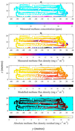
Figure 1.
(a) In situ [CH4]me measurements obtained during flight 2 from the sample data (117 m from the emission source). z is plotted on the vertical axis and y is plotted on the horizontal axis; (b) qme values calculated using [CH4]me values in panel “a”; (c) qmo values modelled on qme values in panel “b.” Panel “b” and panel “c” share a mutual colour scale; (d) Residuals between qme values in panel “b” and qmo values in panel “c.”
Anemometers positioned at various heights were used to infer continuous wind speed (U(z)) and wind direction profiles, along with corresponding wind speed variability (σU(z)) profiles (see Appendix A for further details of the anemometers used). A single mean value of θ was derived for each flight: This was calculated from the average of two-dimensional wind vectors at the height of each [CH4]me measurement. The atmospheric methane mass density (ρ), assuming all of air is methane (in units of kg m−3), was calculated using Equation (1), where M is the molar mass of methane (0.0164 kg mol−1), R is the gas constant (8.314 m3 Pa mol−1 K−1), and T and P are the average temperature and pressure, respectively, for the duration of each UAV flight. Provided that changes in T and P are small, ρ can be assumed to remain constant for the duration of sampling.
2.2. Flux Estimation Using the NGI Method
Here, we describe the procedure applied to each UAV flight from the sample data in order to estimate an initial flux using the NGI method. The qme, as a function of y, z, and x, was calculated using Equation (2), assuming constant ρ. The qme is the emission flux per unit area on the flux plane, derived from each individual [CH4]me measurement (see Figure 1b for flight 2, for example). As Equation (2) requires the concentration enhancement over the background, instrumental resolution (1 ppb for the sample data) can be a limiting factor in the magnitude of fluxes detectable: If fluxes are too low, concentration enhancements may be undetectable.
Equation (3) was used to calculate the uncertainty in qme (Δqme), using the instrumental Allan deviation precision (σAV, specifically 0.00127 ppm for the sample data) and an instrumental uncertainty factor (σi([CH4])) associated with each [CH4]me measurement (see Appendix A for details on σi([CH4])).
The NGI method assumes that spial variability in the time-averaged plume is Gaussian. As a consequence, the NGI method also assumes that the plume is not capped in the z direction by an atmospheric temperature inversion. Conceptually, over an infinite period of randomised sampling, and assuming that the prevailing meteorology does not vary, a Gaussian morphology of qme would be observed as an average of instantaneous sampling. This essentially smooths out the manifestation of turbulence in the time-averaged plume morphology. However, in practice, limited sampling time constraints (particularly for UAV sampling) may potentially lead to the observation of non-Gaussian qme across the sampling plane due to turbulence (see Figure A3 for the example of the sample data). The NGI method is therefore a trade-off between the need to sample for a long enough time to characterise the time-averaged plume as much as possible and the need to minimise the systematic effect of any potential dynamic changes in atmospheric stability, source strength and prevailing meteorology over the course of measurement (parameters which may be derived from complementary specialised UAV sampling [57]). Such competing needs would need to be considered on a case-by-case basis by considering weather forecasts, the local topography and the nature of the expected sources being studied.
An initial flux estimate (Fe) can be derived by fitting qme values to corresponding modelled flux density (qmo) values using an adaptation of the two dimensional Gaussian plume model [76] given by Equation (4). Equation (4) does not include wind speed, as this has been incorporated into qme in Equation (2). An advantage of incorporating wind speed into qme in this way is that variations in wind speed with altitude are incorporated into the measured plume morphology in flux space. An advantage of this method is that it does not require us to assume any stability class, as plume spatial variance is implicitly measured.
σy(x) is the crosswind mixing factor, σz(x) is the vertical mixing factor, yc is centre of the plume in the y direction (based on the actual sampled qme measurements) and h is the emission height.
On an idealised downwind vertical flux plane, perpendicular to θ, σy(x) and σz(x) would be constant for all qme values. However, as σy(x) and σz(x) are both functions of x, they may vary depending on the orientation of the sampling plane, if not perfectly perpendicular to θ. In reality, it is difficult to sample on a perfect perpendicular plane, especially with UAV sampling (see Figure S2 for the example of the sample data), as θ may vary throughout the sampling period. To account for this variability in sampling distance from the source, we assume σy(x) and σz(x) to increase linearly with x (i.e., qme decreases with increasing distance from the source). Though σy(x) and σz(x) may not increase linearly with x over large distances, they can be approximated to be linear functions of x under near-field conditions and where the variation in x remains small (less than 40 m). σy(x) and σz(x) for each stability class were plotted up to 500 m, using the equations found in Turner [76], to test the validity of this assumption (see Figures S4 and S5). This assumption of linearity allowed us to define a crosswind mixing factor evaluated at a distance of 1 m (τy) using Equation (5) and a vertical mixing factor evaluated at a distance of 1 m (τz) using Equation (6). τy and τz are both then scalable factors that can be used to derive σy and σz as a function of x and are therefore applicable to the variable sampling typical of UAV measurement.
As τy and τz are both independent of x, Equation (4) can now be expressed as a three dimensional Gaussian plume, using Equation (7).
One could attempt to solve Equation (7) iteratively for the four unknown constant parameters (F, yc, τy and τz). However, such a solution is not always well constrained by the sampled data. Instead, by utilising the separability of Equation (7), we can place constraints on yc and τy by equating the mean and standard deviation (in the y dimension) of to the equivalent values for . This requires us to remove the vertical (z) component of using Equation (8) to define qme with the z Gaussian component removed (qme,y). As Equation (8) depends on τz, good spatial sampling in the z direction is required in order to derive τz.
yc and τy were then derived analytically from measured data using Equations (9) and (10), respectively, which require each “j” value of z, x and qme,y. Foster-Wittig et al. [39] used an equation similar to Equation (10) to derive σy(x), rather than τy, using downwind concentration measurements acquired at a single position on the ground. As τz in Equation (8) was unknown, Equation (9) and (10) were solved simultaneously along with Equations (7) and (8) as part of the model. A key advantage of calculating yc in this way is that, provided geospatial measurements of a sufficient precision are recorded, the overall systematic accuracy of geospatial sampling is not crucial, as the centre of the plume is derived from spatial measurements relative to each other.
Equations (9) and (10) require good spatial sampling in the y direction, as yc weights the flux contributions to the position of the centre of the measured plume (as sampled), independent of z. This means that if qme at any point in the y direction was equal to 0, it would have no influence in changing the centre of the calculated plume morphology in the y direction. By calculating yc and τy in this way we constrain the model and optimise the flux calculation procedure, such that the only remaining unknown variables in Equation (7) are τz and Fe.
The initialised values of τz and Fe were then evaluated computationally to minimise the sum of squared residuals between all qme and qmo values by solving Equations (7), (9), and (10) simultaneously (as yc and τy are both derived from values of qme,y, which ultimately depend on τz). This was achieved here using the lsqcurvefit function of Matrix Laboratory (MATLAB) 2016a, which applies a least-squares solution to the input data. During the optimisation procedure τz and Fe were both constrained to ensure good parameterisation, as described below, without which the model may produce unrealistic flux results. It was clear that the maximum constraining value of τz (τz,max) had an impact on Fe: If τz,max was too small, τz may have been equal (or almost equal) to τz,max (as illustrated in Figure A4 for example). Furthermore, Fe sometimes failed to stabilise as τz,max increased, regardless of how high τz,max was set to (see Appendix C for further discussion). Therefore, before a final constant Fe result could be produced, the flux evaluation procedure had to be repeated at various values of τz,max. A constant value of Fe was assumed to be produced once incremental changes in τz,max no longer resulted in changes in Fe. Figure 1c gives an example of final constant modelled qmo values for flight 2 from the sample data. Final τz and Fe values were then substituted into Equations (9) and (10) to establish definite values of yc and τy. All resulting yc, τy and τz values for the sample data are given in Table S4.
Once constant values of τz and Fe were acquired for each flight, a measurement uncertainty in Fe (ΔFm) could be calculated through Equation (11), by using each “j” value of qme and Δqme from Equation (3), assuming each Δqme term is uncorrelated.
A total minimum uncertainty (ΔF−) was then calculated using Equation (12) from residuals between each “j” calculation of qme and qmo (see Figure 1d for flight 2, for example). Equation (12) finds the average qme residual, weighted by qme.
The residuals between qme and qmo in Equation (12) incorporate uncertainty in wind direction. Under stable wind conditions, at a constant wind direction, and with infinite spatial sampling, the residual () term in Equation (12) would converge to zero. However, under turbulent (or variable) wind conditions, regardless of sampling spatial extent and sampling duration on the flux plane, the residual () term may be non-zero due to the potential for overlap of various qme measurements at the same point in space at different times. Furthermore, the limited extent of spatial sampling on the flux plane can lead to a flux under-estimate, which must be incorporated into the total maximum uncertainty (ΔF+). This is described in Section 3.
3. Flux Sensitivity Random Walk Simulations
The capability of the NGI method to derive a prescribed modelled point source target flux (Ft) was tested here by simulating randomised near-field sampling of a time-averaged plume. As well as evaluating ΔF+, these simulations can be used for guidance to better plan future sampling, to yield fluxes within some threshold of acceptable uncertainty in operational settings. The simulations were designed to replicate real sampling in the y, z, and x directions (see Figure S6 for an example). Each simulation was based on parameters retrieved when calculating Fe from the NGI model (yc, h, τy and τz), the orientation of the qme sampling plane in the x direction and the spatial distribution of qme sampling. Each simulation was constrained by the maximum bounds of qme sampling.
Each simulation was initialised from a random y and z position on the sampling plane (point 1 in Figure 2, where Figure 2 is a schematic diagram of a random walk). The distance of each step in the random walk was constant (on a plane perpendicular to x), with a length (L) equal to the average distance between successive real measurement points. In order to replicate changes in sampling direction on the plane perpendicular to x, an exponential probability distribution was fitted to the absolute change in angle between each successive measurement step (see insert in Figure 2). This probability distribution was used to model the change in angle (in magnitude but not in sign) between each successive step in the random walk (δθ), from an initial random direction (θR). At the sampling plane boundary, the random walk direction was deflected by an angle of either 135° or 225°, provided that the random walk remained within the spatial confines of sampling. The orientation of the simulated sampling plane in the x and y direction, relative to mean wind direction, was chosen to match the orientation of the sampling plane from real sampling (see supplement for details). Simulated qme values were then generated for each step in the random walk using Equation (7), where Fe was replaced by Ft and qmo was replaced by qme.
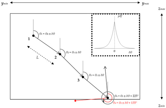
Figure 2.
A schematic of the random walk simulation with an example δθ exponential probability distribution function (pdf) in the top right hand corner. Each step in the random walk is numbered from 1 to 4. Upon reaching the plane boundary at point 4, a deflection of 225° was applied, since a deflection of 135° (red square) failed to keep the random walk within the confines of spatial sampling. The sampling plane spans from the minimum real y measurement (ymin) to the maximum real y measurement (ymax) and from the minimum real z measurement (zmin) to the maximum real z measurement (zmax).
For each test described in the following sections, multiple independent random walks (and simulated qme values) were generated from scratch, for either a single fixed simulated sampling time (t) or for various values of t. For each random walk in each test, t was adjusted by altering the total number of steps in the random walk. Each individual random walk sampled the flux plane following a different route, making each random walk unique. A virtual flux estimate (Fe,v) was calculated from each random walk (which is a function of t), following the NGI method. As modelled fluxes can fail to stabilise when τz,max is equal to model output value of τz, five conditions were put in place to ensure that the model had stabilised. These conditions are described in detail in Appendix B.
3.1. Upper Flux Uncertainty Bounds
The difference between Ft and simulated flux (Fe,v) was assessed at a fixed simulated sampling time corresponding to the duration of actual sampling for each flight in the sample data. Fluxes for this analysis were derived by continuously repeating a random walk simulation to accumulate a large number (180 for the sample data) of virtual fluxes (see green lines in Figure 3a for example). The average value of Fe,v (, solid green line in Figure 3a) was negatively biased from Ft due to three independent effects.
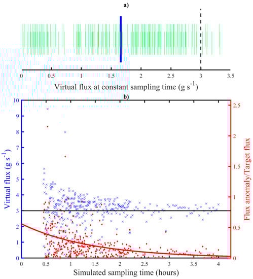
Figure 3.
(a) Fe,v at fixed t (green vertical lines), simulating flight 3 from the sample data, with , (blue vertical line) and Ft (dashed black vertical line) also shown. (b) Bias corrected Fe,v values as a function of t (blue crosses), plotted against left-hand axis, with Ft (black line) also shown. Flux anomalies as a fraction of Ft (red diamonds) are plotted against the right-hand axis with an exponential fit plotted as a red line (see text for further details).
- The simulated sampling extent was restricted as a consequence of the managed sampling strategy, resulting in an inadequate characterisation of the entire emission plume.
- Sampling was physically restricted in the z direction due to the non-zero height of the air inlet (as was the case for our UAV platform), resulting in an under-sampled area very close to the ground.
- The random walk was time-limited, resulting in an incomplete exploration of the available flux plane and hence, sampling gaps, leading to a residual negative flux bias.
These effects collectively result in a lack of spatial sampling across the flux plane and thus insufficient sampling with which to calculate τy and τz, which are derived here from measurements of qme across the sampling plane. In theory, these effects can be alleviated with infinite spatial sampling on an infinitely sized sampling plane, but this cannot realistically be achieved from a UAV (or any) sampling platform. These three effects were incorporated into ΔF+ by adding the deviation of Fe,v from Ft to ΔF−, using Equation (13).
Thus, Figure 3a shows that as a consequence of the three effects outlined above, the NGI method can result in a large variation in flux estimation with the potential for a large negative flux bias.
3.2. Uncertainty Sampling Thresholds
By gradually increasing t in each simulation, the convergence of Fe,v towards Ft was assessed (blue crosses in Figure 3b, for example). This makes it possible to analyse the limiting uncertainty that exists in Fe,v as a function of t, due to the random error associated with the NGI method itself rather than due to the quality of sampling. This test is only valid for relatively non-variable atmospheric conditions, as it assumes the time-averaged plume to be static. For each flight from the sample data, independent random walks of up to four hours were generated. A simulated scale factor as a function of t was applied to these fluxes to correct for the inherent negative bias that occurs as a function of t (see previous section). This scale factor was derived by repeatedly performing random walks at a range of fixed sampling times to quantify the average negative flux bias as a function of t (see supplement for details). Without applying this scale factor, Fe,v gradually increased towards Ft, as a function of t (see Figure S7 for example). Following the application of this scale factor, the absolute difference between bias-corrected Fe,v and bias-corrected was used to find the flux anomaly (A) as a function of t (red diamonds in Figure 3b, for example). The decrease of A with increasing t represents a reduction in the fundamental methodological uncertainty due to a greater understanding of the time-averaged plume morphology. The flux anomalies in Figure 3b show that with a sufficient sampling duration, the fundamental methodological uncertainty can gradually be reduced until it converges towards zero.
The flux anomaly was assumed to decrease exponentially with t, from which a fit could be produced using Equation (14) to define an anomaly coefficient, α, and an anomaly decay constant, β (see Table S5 for values for the sample data). This fit was weighted to take into account fewer simulations at longer t, such that the fit was evenly applied as a function of t.
By setting t in Equation (14) to the duration of each UAV flight in the sample data and by setting Ft to Fe, the limiting uncertainty (Af) associated with each flight could be derived. Af represents the inherent limiting uncertainty, determined by the sampling strategy (assuming non-variable atmospheric conditions), which decreases as a function of t. Alternatively, Equation (14) could be rearranged to make t the subject. Then, by setting A to a specified target fraction of Ft, the minimum time required to surpass a target limiting uncertainty threshold could then be derived. This may be useful to decide future UAV sampling durations within a desired minimum confidence level. For example, setting A to 1% of Ft yielded the 1% fundamental uncertainty sampling threshold (t1%). The use of limiting confidence timescales is only valid if non-variable atmospheric conditions are assumed. Therefore, the threshold time must be comparably smaller than the timescale of prevailing meteorological change.
3.3. Testing the NGI Method
Finally, virtual flux simulations were used to test the NGI method in principle. First, the flux plane was extended to mitigate biases due to the limited size of the sampling plane. The maximum sampling extent in the z direction was doubled, and the left and right x bounds were also doubled (resulting in an increase in the size of the original sampling plane by a factor of approximately 6). Furthermore, the flux plane was extended down to ground level. The total simulated sampling time (t) was then set to an arbitrary (approximately 72 h) sampling time across the extended flux plane to mitigate the effects of limited spatial sampling coverage, as well as to minimise the limiting uncertainty discussed in the previous section. The simulation was then repeated 60 times for each flux. Average Fe,v results deviated from Ft by (−0.7 ± 0.5)%, (see Table S6 for results using the sample data). This test validates the utility of the NGI method by confirming that it accurately yields Ft, in principle.
4. Results and Future Guidance
The sample data used to develop the NGI flux quantification method described here was acquired using the controlled release of natural gas (supervised by the NPL) at two flux rates ((1.5 ± 0.1) g s−1 and (3.0 ± 0.2) g s−1). The NGI fluxes for each of eight UAV flights are displayed in Figure 4, along with flux uncertainty bounds, expressed as a percentage of the NPL controlled release facility (CRF) reported emission flux (see Table S1 for individual flux values for each flight). All values of Fe, ΔF+, and ΔF− are given in Table S7. As this was a preliminary study, regardless of uncertainty, we note that most NGI fluxes calculated for the sample data exceeded CRF fluxes due to the biased nature of our sampling. Though potential sources of negative bias due to sampling limitations are incorporated into the NGI flux uncertainty range, the effects of positive bias are clearly dominant here. One such source of positive bias is the targeted sampling strategy described in Section 2.1, resulting in plume chasing. The NGI method inherently assumes that the measurements constitute an unbiased sample of the time-averaged Gaussian plume. However, during the acquisition of the sample data, the UAV was directed towards the perceived position of the instantaneous plume to maximise in-plume sampling. Future studies adopting this technique should avoid chasing the plume in this way, as it results in the over-representation of in-plume measurements, which biases NGI fluxes. Another possible source of bias may be wind measurements; if the winds at the location of the anemometers were systematically different from those at the UAV sampling locations, this would have a direct impact on the calculated fluxes.
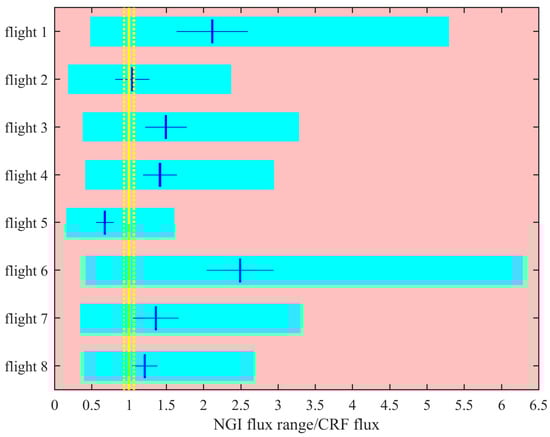
Figure 4.
Near-field Gaussian plume inversion (NGI) flux results for the sample data, expressed as a ratio to the controlled release facility (CRF) emission flux. The calculated uncertainty flux range (from ΔF− to ΔF+) is expressed as a cyan bar and Fe is a vertical blue line for each flight. The ΔFm range is expressed as a horizontal blue line. The solid yellow line represents Fe being equal to the CRF flux.
The flux biases in this work can be compared to a previous study by Brantley et al. [35], which quantified the controlled release of methane using Gaussian plume modelling of stationary measurements; their method both overestimated and underestimated fluxes by between −87% and +184%, respectively. The wide variation in fluxes acquired by Brantley et al. [35] highlights issues similar to those experienced in other studies using near-field concentration measurements in turbulent (non-ideal) conditions with time-limited sampling, i.e. that sampling a non-disperse emission plume can result in large flux uncertainty.
Though seven out of eight Fe values were above the CRF flux due to the biased sampling, all reported CRF fluxes fell within the full UAV flux uncertainty range, which spanned between (−76 ± 5)% and (+132 ± 15)% of Fe. Flight 6 had a particularly high NGI flux uncertainty range due to a high quantity of sampling at the edge of the plume (see Figure A3), rather than the centre. Failure to adequately sample the centre of the plume can result in a much larger false plume being extrapolated, using the NGI method, in certain cases. It is clear from Figure 4 that the ΔFm uncertainty range was dwarfed by the extended uncertainty range, which was higher in all cases due to the dominating effect of the uncertainty in wind direction. To assess the various sources of UAV sampling uncertainty in ΔFm, a sensitivity test was performed (see Table S8). The principal source of uncertainty in ΔFm was from uncertainty in wind speed (see Table S8). An improved understanding of the temporal variability of the two-dimensional wind field on the flux plane, either by on-board UAV wind measurement or by other means, would serve to reduce this dominant source of uncertainty. However, the combined effects of instrumental uncertainty and uncertainty in the background were small compared with effects associated with natural variability in the wind field, which suggests that instruments such as the UGGA are suitable for measurement of fluxes similar to those in our study at similar downwind distances.
We compared the UAV flux uncertainties from the sample data to other methods. Seven of the eight TDM flux estimates which were acquired simultaneously during this study (see Table S1) agreed with the CRF, within uncertainty, with an average bias of (−2 ± 10)%. The average uncertainty in individual TDM fluxes (through comprehensive uncertainty budgeting) was ±21% [75]. In a different study using mass balance box modelling, Krautwurst et al. [42] derived the emission flux from a single landfill site based on both remote sensing column-concentration aircraft measurements and in-situ aircraft concentration measurements, with average flux uncertainties of ±34.5% and ±19.7%, respectively. Elsewhere, the uncertainty in fluxes obtained by Nathan et al. [73], using mass balance box modelling of polar coordinates and kriging to quantify the emission flux from a natural gas compressor station, was ±55%, although we dispute the use of kriging as an appropriate tool in that case. Yacovitch et al. [37] used a Gaussian plume inversion of ground based measurements to quantify emission fluxes from oil and gas infrastructure facilities, which used σy(x) and σz(x) values based on stability classes (rather than derived from qme), with asymmetric 95% confidence uncertainties of between −33.4% and +334%. Therefore, we conclude that the NGI method using UAV sampling can be a competitive tool for rapid flux assessments of emitter facilities, assuming sampling from point source emitters. While the uncertainties we derived are comparatively large, the NGI method is able to derive rapid flux estimates from time-limited UAV sampling.
Though we report large NGI flux uncertainties for the sample data, alternative techniques such as mass balance box modelling cannot be used reliably to quantify fluxes using off-site downwind UAV sampling. To explain these conclusions, we have assessed the suitability of two mass balance box modelling approaches here. Mass balancing using geospatial kriging cannot be used, as kriging requires the interpolation of time-invariant downwind sampling. In this work, the qme plume sampled by a UAV near-to-source was not time invariant due to turbulent fluctuations in the position of the plume on the sampling plane. Though kriging may be used in principle in stable (non-turbulent) wind conditions, stable winds are unlikely when sampling with a UAV near-to-source. Alternatively, mass balancing may be applied by averaging qme into equally sized grid squares on a plane perpendicular to mean wind direction. However, this requires the entire extent of the time-averaged plume to be captured by the UAV, down to ground level. It also requires dense spatial sampling without any large sampling voids. While the method of grid square averaging may again be possible in principle, in order to produce sufficiently dense spatial sampling, a longer UAV sampling duration would be required compared to the sampling presented here. Furthermore, sampling down to ground level can be problematic, as it relies on the position of the air inlet on a UAV being close to the base of the UAV, and effects or prop-wash may be expected. Thus, we suggest that neither mass balance box modelling approach can be used for the type of near-field UAV sampling presented here—rather, the NGI method is a suitable flux quantification technique for near-field UAV sampling.
Future UAV flight sampling should be planned to minimise flux uncertainties, including potential sources of bias. The random walk simulations were used to generate values of Af for each flight from the sample data, which are given in Table 1. They show that regardless of measurement uncertainty, wind variations and the spatial extent of sampling, an average (58 ± 30)% limiting threshold uncertainty remains due to limited spatial coverage on the sampling plane. The random walk simulation could also be applied to obtain t0.01 required to surpass a 1% uncertainty threshold, assuming good randomised sampling of a static plume. It is clear that the theoretical t0.01 values in Table 1 (of at least 5 h) are unrealistic for UAV sampling, which cannot practically be achieved by a single light UAV platform over the timescale of a single flight (typically < 30 min using current battery technology constraints). However, using multiple UAV flights or tethered power (for uninterrupted sampling) may increase sampling time. The t0.01 values are only valid when sampling in stable atmospheric conditions with a relatively non-variable wind direction. In reality, over the t0.01 times given in Table 1, non-variable atmospheric conditions are unlikely, leading to the potential for large NGI uncertainties from UAV sampling. Therefore, if additional UAV sampling is used, a compromise sampling time must be reached over which atmospheric conditions change very little while the sampling period is maximised to minimise uncertainty.

Table 1.
Af as a fraction of Fe and t0.01 for each unmanned aerial vehicle (UAV) flight in the sample data.
5. Conclusions
A near-field Gaussian plume inversion was used to quantify methane emission fluxes from eight UAV flights downwind of a controlled emission source. The new NGI method takes into account the imperfect orientation of a two-dimensional vertical sampling plane perpendicular to mean wind direction. The number of unknown parameters in the inversion was reduced by deriving constraining parameters in the y direction from flux density measurements. Uncertainties were derived from measurement uncertainty as well as the difference between measured and modelled flux density results. The upper flux uncertainty bound was further enhanced by taking into account the lack of spatial sampling extent, using a random walk simulation of sampling. The random walk sensitivity tests also highlight areas of future improvements to the sampling strategy, which will be a focus of future experimental work. They also highlight the importance of evenly-distributed sampling of an adequate duration and the need for a sufficiently large sampling plane.
We suggest that the NGI method is a highly suitable technique that can be used to accurately quantify emission fluxes from static point sources of both methane and other trace gas sources, with measurement potential by UAVs. This allows for the full potential of near-field in-situ spatial sampling that UAVs provide to be realised. Though we acknowledge the magnitude of uncertainty may be high over a single UAV flight, the NGI method allows for rapid flux estimation with a defined maximal uncertainty. Mass balance box modelling may not be suitable for UAV in-situ sampling as it requires either the sampling of a time invariant plume or dense spatial sampling of a time-averaged plume. Though the NGI method yielded highly successful results when using a random walk simulation, the preliminary fluxes from the sample data resulted in high uncertainties. It is suggested that future studies that utilise the NGI method should adopt a sampling strategy that addresses the potential sources of bias highlighted here by ensuring that plume-chasing is avoided and by ensuring that sampling is sufficient to capture the entire extent of the time-averaged plume.
With the possibility of in-situ UAV wind measurements in future, there is further scope to improve flux accuracy. Future progress may be made by mounting an in-situ methane sensor directly onto a UAV, to eliminate issues associated with the use of a tether. Such improvements and further near-field sampling studies using the NGI method can play an important role in efforts to improve emission inventories. Additionally, UAVs may be used to add a vertical sampling dimension to the TDM technique using in-situ tracer gas detection. To conclude, a Gaussian plume inversion flux quantification method, using in-situ [CH4] measurements of a sub-ppm precision, has been characterised here and future improvements are viable. This permits future studies of unknown well-defined sources (such as landfill sites, oil and gas infrastructure facilities, or herds of cattle) to be conducted using the method, depending on the precision of instrumentation.
Supplementary Materials
The following are available online at https://www.mdpi.com/2073-4433/10/7/396/s1, Table S1: Reported CRF methane flux releases with the time duration of continuous methane emission given in seconds past midnight (spm), local time (GMT); Figure S1: A photograph of the UAV platform at rest (without battery), with the PFA tubing pointing upwards; Table S2: UAV flight details and flight track colours; Figure S2: Aerial view of the three emission source locations (black dots) and flight tracks (coloured dots); Figure S3a: A histogram of methane concentration measurements obtained throughout flight 1 from the sample data; Figure S3b: A histogram of the lowest concentration measurements from flight 1 (red bars) with 15-bin-averages (green line) and log-normal function fit (blue line) plotted against the left hand axis; Table S3: Calculated background concentrations for each flight from the sample data; Figure S4: σy(x) plotted for various stability classes (red lines) using the equations in Turner (1994); Figure S5: σz(x) plotted for various stability classes (red lines) using the equations in Turner (1994); Table S4: yc, σy(x) and σz(x) for each UAV flight from the sample data and the average parallel distance of the sampling plane from the emission source; Figure S6: An example of a virtually-generated random walk to replicate flight 8 from the sample data, with the duration of the random walk set to the equivalent time period (21 min); Figure S7: Fe,v, i values, simulating flight 3 from the sample data, as a function of t (blue crosses), plotted against left-hand axis, with Ft (black line) also shown; Table S5: Flux convergence parameters required to approximate the fundamental threshold uncertainty associated with flux measurements as a function of sampling time, which are unique for each flight in the sample data; Table S6: Average virtual test Fe values for each flight in the sample data with eight hours of random sampling of a static plume; Table S7: Initial flux values and corresponding fractional lower and upper uncertainty bounds, for each flight from the sample data; Table S8: A comparison between ΔF−me and ΔF−mo for each flight from the sample data, as a fraction of ΔF−; Table S9: A comparison between ΔF−me,U(z), ΔF−me,ρ and ΔF−me,ib for each flight from the sample data, as a fraction of ΔF−me.
Author Contributions
Formal analysis, A.S., G.A. and J.R.P.; funding acquisition, G.A. and M.B.; investigation, A.S., G.A., H.R., P.I.W., J.H., A.F., R.R., K.K., P.H., T.C.R.-W., R.B., C.S. and M.B.; methodology, G.A., J.H., K.K. and M.B.; resources, G.A. and P.H.; software, A.S.; supervision, G.A.; writing—original draft, A.S. and G.A.; writing—review and editing, A.S., G.A., J.P., H.R., P.W., J.H., A.F., R.R., T.C.R.-W., R.B. and C.S.
Funding
The Natural Environment Research Council (NERC) funded AS’s PhD studentship through the EAO doctoral training partnership (NERC grant reference NE/L002469/1). NERC provided contributions in kind, through access, equipment and expertise through the GAUGE programme (NERC grant reference NE/K00221X1/1). The UAV sampling and controlled methane release was funded by the Environment Agency.
Acknowledgments
We thank the Met Office and their staff at the Meteorological Research Unit in Cardington for allowing us to use their site and cooperating with our research.
Conflicts of Interest
The authors declare no conflict of interest.
Appendix A
Four NPL CRF releases of natural gas (provided by BOC Ltd., Guilford, Surrey, UK) were conducted at the UK Met Office’s Meteorological Research Unit (MRU) in Cardington, Bedfordshire, UK (longitude: 0°25′21″ W; latitude: 52°6′32″ N), on 2 November 2016 and 3 November 2016. Further details of the CRF are given in the supplement. The operating site is a mown grass field with single-storey office facilities. The site has a maximal length of ~600 m and a maximal width of ~400 m. During each flight, fluxes were released at one of two prescribed emission rates from three locations around the site from a ~6.2 m tower, selected for optimal downwind UAV sampling for the prevailing wind direction at the time of each flight experiment (see Table S1 for release details). The MRU was ideal for the acquisition of sample data, as it was distant (>5 km) from any expected significant sources of off-site (and therefore interfering) methane such as large towns, cities or landfill sites.
Four 10 Hz sonic 3D anemometers (HS-50 Horizontal-Head Ultrasonic Anemometer, Gill Instruments Limited) were positioned on the site at heights of 2, 10, 25, and 50 m above ground level. The average wind speed and wind direction for the duration of each UAV flight was interpolated (using a shape-preserving piecewise cubic interpolation) as a function of z to derive a continuous wind profiles as a function of height for each flight. Thus, θ took into account wind shear by interpolating wind speed measurements from the four anemometer towers. The variability in wind speed measured by each anemometer was interpolated as a function of altitude to produce a continuous uncertainty profile.
During each controlled release, a modified DJI Spreading Wings S900 hexacopter UAV (Figure A1) was manually piloted by experienced personnel on the ground and guided for sampling by an assistant, acting as a lookout. The pilot had a qualification in UK airspace legislation and was experienced and competent in flying small UAVs. As the UAV was used for scientific (rather than commercial) purposes, a pilot qualification from the Civil Aviation Authority (CAA) was not required, in accordance with UK airspace legislation. The UAV flew at an average speed of (0.4 ± 0.1) m s−1. It was directed mid-flight to capture as much of the plume as possible based on mid-flight knowledge of the plume position, using the release of smoke flares. Though the UAV was limited to a physical height of 150 m (i.e., the length of the tubing), the UAV only flew up to (24 ± 3) m to ensure extensive vertical sampling of the emission plume; the maximum height of the plume was determined using a visible plume observed from the release of smoke flares. Prior to each flight, the CRF release point and UAV sampling area were defined in a planning and safety briefing, using forecasts of wind direction to optimise the available operational sampling area around on-site buildings and obstructions (such as the anemometer masts) and to ensure minimum UAV safety distances (50 m) from personnel and property beyond the pilot’s control, as defined by CAA regulations [77]. Each flight track was roughly aligned in a vertical sampling plane perpendicular to θ by manual piloting, (90 ± 30) m from the source. However, there was a clear inclination between the sampling plane and the plane perpendicular to θ, which was accounted for in the NGI method. UAV longitude, latitude, and altitude were recorded at a 5 Hz frequency by an on-board Pixhawk computer (independent of the on-board flight controller), connected to a Cirocomm 00BY satellite geolocation antenna, which was secured to the top of the UAV. For a continuous stationary 60 s sampling period, x, y, and x varied with a standard deviation of no more than ±0.15 m. Thus, the precision of the sensor was suitable for our flux quantification purposes.

Figure A1.
(a) The DJI Spreading Wings S900 UAV, mid-flight, with a 150 m long tether, connected to an instrument on the ground; (b) The UAV on the ground, prior to flight. Notice the air inlet above the plane of the propellers.
Figure A1.
(a) The DJI Spreading Wings S900 UAV, mid-flight, with a 150 m long tether, connected to an instrument on the ground; (b) The UAV on the ground, prior to flight. Notice the air inlet above the plane of the propellers.

[CH4] was recorded at ~1 Hz by securing a 150 m long, 4.76 mm inner diameter perfluoroalkoxy alkane (PFA) tube to the UAV, through which air was pumped (at a continuous flow rate of 0.5 litres per minute) to a commercially available 15 kg UGGA methane sensor (Figure A3) which was fixed on the ground, operating at a fixed pressure of 140 Torr. The UGGA uses off-axis integrated cavity output spectroscopy to derive concentration measurements (see Baer et al. [78] and Paul et al. [79] for full spectroscopic details): A 1650 nm tuneable laser is reflected between two mirrors in a high finesse cavity, with the output spectrum integrated as a function of wavelength, to derive concentration using the Beer–Lambert law. Live concentration measurements from the UGGA could be viewed on a computer screen on the ground, where data was saved for subsequent analysis. The UGGA was powered in the field using a 12 V lead-acid battery. Though the ground-based sampling used here allows for high-precision heavier instrumentation (like the UGGA) to be used, it also suffers a number of drawbacks, such as lag time through the tubing (which we account for) and the kinking of the tube, resulting in air failing to reach the sensor on the ground (which we omitted during flux analysis). A small loop at a fixed position on the tubing was fastened to the same point beneath the UAV, prior to flight, to ensure consistency in the length of the tubing between flights. In this work, the tip of the inlet was positioned ~20 cm above the plane of the rotor blades to ensure that sampled air was not disturbed by propwash or air flow through the rotors (see Zhou et al. [66] for example). Computational fluid dynamics (CFD) model simulations (not shown) demonstrated that the inlet was positioned sufficiently far enough away from the rotors to exclude this. The CFD simulations showed that there was no significant vertical disturbance to air a sufficient distance above the plane of the propellers.

Figure A2.
(a) The Ultra-portable Greenhouse Gas Analyzer (UGGA) with its lid closed and an air inlet attached; (b) the UGGA with its lid open.
Figure A2.
(a) The Ultra-portable Greenhouse Gas Analyzer (UGGA) with its lid closed and an air inlet attached; (b) the UGGA with its lid open.

The accuracy of UGGA concentration measurements was enhanced using a post-flight water vapour correction (see O’Shea et al. [80] for details). Measurements were then further calibrated using a two term linear correction (derived from an average of eight calibration procedures, described in detail by Pitt et al. [81]), such that dry methane concentration measurements were robustly traceable to the World Meteorological Organization greenhouse gas calibration scale [82].
Equation (A1) was used to calculate σi([CH4]) values specific to the UGGA (required to calculate of uncertainty in qme in Equation (3)).
GF was the average of eight previously calculated gain factors, and σGF was its corresponding standard deviation. The ratio between σGF and GF was 0.00282. WC([CH4]) is a water correction factor which was directly applied to raw concentration measurements and is a function of water concentration. σWC was the uncertainty associated with the water correction.
Each longitude, latitude, and altitude measurement from the UAV was interpolated onto the lower frequency UGGA time grid (avoiding extrapolation of [CH4] measurements). UGGA measurements were also corrected to the UAV sampling time by calculating the lag time (τlag), in order to geospatially reference UGGA measurements (by subtracting τlag from the UGGA time-stamp), to account for the time taken for air to travel through the tubing. τlag was tested prior to and immediately following each flight (by blowing into the inlet and timing the carbon dioxide concentration response). τlag varied flight-to-flight with a mean (and maximal range from flight-to-flight) of (300 ± 10) s. τlag was measured before and after each flight and found to be constant. However, it gradually varied throughout the day. This small variation may have been due to changes in ambient pressure, which slightly alter the mass flow rate through the pump in the UGGA. τlag was assumed to remain constant throughout each flight, as was it controlled by the strength of the pump (operating at a controlled pressure), with ambient pressure changes assumed to be minimal over the short period of each UAV flight.
Appendix B
Geospatially mapped [CH4]me measurements for each UAV flight have been plotted in Figure A3, where z has been plotted on the y-axis, and y (obtained by rotating the distance from the Prime Meridian and the Equator, respectively, by θ) has been plotted on the x-axis. For each of the eight flight tracks shown in Figure A3, the CRF emission point was from a tower ~6.2 m above ground level. For each flight bar flight 4, the highest concentration measurements were typically detected by the UAV to the left of the position of the emission source projected by θ onto the sampling plane (set to 0 m in the y direction in Figure A3). The CRF emission flux for flights 1–6 was (3.0 ± 0.2) g s−1, while the emission flux for flights 7 and 8 was (1.5 ± 0.1) g s−1. Methane was released at these flux rates throughout the period of sampling.

Figure A3.
In-situ [CH4]me measurements obtained by the UAV for the sample data, plotted according to geolocation corrected for time lag. Flights are numbered according to assigned flight numbers given in Table S2 in the supplement. A logarithmic color scale has been used. z is plotted on the vertical axis and y is plotted on the horizontal axis.

The highest recorded concentrations during flight 1 were observed between ~−10 m and ~−35 m horizontally, where the UAV clearly intersected the centre of the advecting emission plume. The highest concentration measurements from flight 2 were made nearer to ground level from between ~−25 m and ~+15 m horizontally. These concentration measurements were the highest experienced during all eight flights (~25 ppm). High concentration measurements were also detected during transects ~10 m above ground level, with some to the very right (~+30 m) of the extent of UAV sampling. The dominating high concentration measurements acquired from flight 4 were made between ~0 m and ~+20 m horizontally.
Flight 3 featured the narrowest sampling by the UAV, with the far left side (>−25 m) mostly composed of background (~2 ppm) measurements. The highest concentration measurements were randomly distributed towards the centre of the sampling plane. Flight 8 was similar with high concentration measurements overlapping background measurements between ~−70 m and ~−20 in the y direction, with the highest measurements made at ground level between ~−60 m and ~−50 in the y direction.
The highest concentration measurements observed during flight 5 occurred in a small area near ground level at ~−48 m in the y direction. Other moderately high measurements were scattered between ~−60 m and ~−20 m in the y direction. Similarly, the highest concentrations observed in flight 6 occurred in a small area near ground level ~−69 m in the y direction to the very edge of the extent of UAV sampling. The highest concentrations in flight 7 were overlapped by lower (but still elevated relative to background) concentrations between the ground and ~15 m above ground level at ~−50 m in the y direction. The plume was intersected at other positions (between ~−30 m and ~−60 m in the y direction).
Appendix C
In order to derive Fe using the NGI method, Equations (7), (9) and (10) are required simultaneously. The model could be initialised using prior values of Fe and τz, along with maximum and minimum constraints to both of these values. When running the model under various constraining parameters, it was observed that τz was equal to τz,max, when τz,max was low (see Figure A4 for example). As a consequence, the model failed to produce a stable value of Fe, representing the true flux. This was because the model’s sampling space was constrained, which constrained an optimum value of Fe from being attained: The size of the plume in the z direction was restricted from expressing its full magnitude at low τz, potentially suppressing Fe. This issue was resolved by incrementally increasing τz,max until it was clear that any further increase in the τz,max would fail to increase τz. Once τz had stabilised (as a function of increasing τz,max), it was clear that Fe also stabilised (see Figure A4 for example), provided that the maximum containing value of Fe was also sufficiently large. Until such a point could be reached, Fe was rejected.
Unsuitable fluxes were manually rejected during the initial flux quantification procedure. However, for the random walk simulations, a more robust automated procedure was required with which to accept or reject the final NGI Fe values (i.e., corresponding to the highest value of τz,max), using the following five conditions
- 0.98 times the final τz value must be less than the penultimate τz value (which ensures τz has stopped increasing).
- The final τz value must be less than 0.98 times τz,max for that modelled run (which ensures that τz,max has sufficiently exceeded τz).
- The penultimate τz value must be less than 0.98 times τz,max for that modelled run (which ensures that τz,max has sufficiently exceeded τz).
- The final Fe value must be less than 0.98 times the maximum constraining Fe value (which ensures that Fe has stopped increasing).
- The penultimate Fe value must be less than 0.98 times the maximum constraining Fe value (which ensures that Fe has stopped increasing).
The first three conditions ensured that τz has stabilised. The fourth and fifth conditions ensured that the maximum constraining Fe value was sufficiently large to avoid it constraining Fe.

Figure A4.
The variation in the modelled output value of Fe (green dots plotted against the left-hand axis) and τz (red dots plotted against the right-hand axis) as a function of τz,max, for flight 7 from the sample data. The maximum value of τz is plotted as a green line against the right-hand axis.

References
- Shindell, D.T.; Faluvegi, G.; Koch, D.M.; Schmidt, G.A.; Unger, N.; Bauer, S.E. Improved Attribution of Climate Forcing to Emissions. Science 2009, 326, 716–718. [Google Scholar] [CrossRef] [PubMed]
- Etminan, M.; Myhre, G.; Highwood, E.J.; Shine, K.P. Radiative forcing of carbon dioxide, methane, and nitrous oxide: A significant revision of the methane radiative forcing. Geophys. Res. Lett. 2016, 43, 12614–12623. [Google Scholar] [CrossRef]
- Loulergue, L.; Schilt, A.; Spahni, R.; Masson-Delmotte, V.; Blunier, T.; Lemieux, B.; Barnola, J.M.; Raynaud, D.; Stocker, T.F.; Chappellaz, J. Orbital and millennial-scale features of atmospheric CH4 over the past 800,000 years. Nature 2008, 453, 383–386. [Google Scholar] [CrossRef] [PubMed]
- Earth System Research Laboratory ESRL Global Monitoring Division—Global Greenhouse Gas Reference Network. Available online: https://esrl.noaa.gov/gmd/ccgg/trends_ch4/ (accessed on 24 January 2017).
- Rigby, M.; Prinn, R.G.; Fraser, P.J.; Simmonds, P.G.; Langenfelds, R.L.; Huang, J.; Cunnold, D.M.; Steele, L.P.; Krummel, P.B.; Weiss, R.F.; et al. Renewed growth of atmospheric methane. Geophys. Res. Lett. 2008, 35, L22805. [Google Scholar] [CrossRef]
- Saunois, M.; Bousquet, P.; Poulter, B.; Peregon, A.; Ciais, P.; Canadell, J.G.; Dlugokencky, E.J.; Etiope, G.; Bastviken, D.; Houweling, S.; et al. The global methane budget 2000–2012. Earth Syst. Sci. Data 2016, 8, 697–751. [Google Scholar] [CrossRef]
- Nisbet, E.G.; Dlugokencky, E.J.; Manning, M.R.; Lowry, D.; Fisher, R.E.; France, J.L.; Michel, S.E.; Miller, J.B.; White, J.W.C.; Vaughn, B.; et al. Rising atmospheric methane: 2007–2014 growth and isotopic shift. Glob. Biogeochem. Cycles 2016, 30, 1356–1370. [Google Scholar] [CrossRef]
- Dlugokencky, E.J.; Nisbet, E.G.; Fisher, R.; Lowry, D. Global atmospheric methane: Budget, changes and dangers. Philos. Trans. R. Soc. A 2011, 369, 2058–2072. [Google Scholar] [CrossRef]
- Prather, M.J.; Holmes, C.D.; Hsu, J. Reactive greenhouse gas scenarios: Systematic exploration of uncertainties and the role of atmospheric chemistry. Geophys. Res. Lett. 2012, 39, L09803. [Google Scholar] [CrossRef]
- Saunois, M.; Jackson, R.B.; Bousquet, P.; Poulter, B.; Canadell, J.G. The growing role of methane in anthropogenic climate change. Environ. Res. Lett. 2016, 11, 120207. [Google Scholar] [CrossRef]
- Bogner, J.; Pipatti, R.; Hashimoto, S.; Diaz, C.; Mareckova, K.; Diaz, L.; Kjeldsen, P.; Monni, S.; Faaij, A.; Gao, Q.X.; et al. Mitigation of global greenhouse gas emissions from waste: Conclusions and strategies from the Intergovernmental Panel on Climate Change (IPCC) Fourth Assessment Report. Working Group III (Mitigation). Waste Manag. Res. 2008, 26, 11–32. [Google Scholar] [CrossRef]
- Allen, G. Rebalancing the global methane budget. Nature 2016, 538, 46–48. [Google Scholar] [CrossRef] [PubMed]
- Johnson, K.A.; Johnson, D.E. Methane Emissions from Cattle. J. Anim. Sci. 1995, 73, 2483–2492. [Google Scholar] [CrossRef] [PubMed]
- Hodgkinson, J.; Tatam, R.P. Optical gas sensing: A review. Meas. Sci. Technol. 2013, 24, 012004. [Google Scholar] [CrossRef]
- Allen, G.; Gallagher, M.; Hollingsworth, P.; Illingworth, S.; Kabbabe, K.; Percival, C. Feasibility of Aerial Measurements of Methane Emissions from Landfills, 1st ed.; Environment Agency: Bristol, UK, 2014.
- Mønster, J.; Kjeldsen, P.; Scheutz, C. Methodologies for measuring fugitive methane emissions from landfills—A review. Waste Manag. 2019, 87, 835–859. [Google Scholar] [CrossRef] [PubMed]
- Harper, L.A.; Denmead, O.T.; Flesch, T.K. Micrometeorological techniques for measurement of enteric greenhouse gas emissions. Anim. Feed Sci. Technol. 2011, 166, 227–239. [Google Scholar] [CrossRef]
- Xu, L.; Lin, X.; Amen, J.; Welding, K.; McDermitt, D. Impact of changes in barometric pressure on landfill methane emission. Glob. Biogeochem. Cycles 2014, 28, 679–695. [Google Scholar] [CrossRef]
- Denmead, O.T.; Harper, L.A.; Freney, J.R.; Griffith, D.W.T.; Leuning, R.; Sharpe, R.R. A mass balance method for non-intrusive measurements of surface-air trace gas exchange. Atmos. Environ. 1998, 32, 3679–3688. [Google Scholar] [CrossRef]
- Karion, A.; Sweeney, C.; Pétron, G.; Frost, G.; Hardesty, R.M.; Kofler, J.; Miller, B.R.; Newberger, T.; Wolter, S.; Banta, R.; et al. Methane emissions estimate from airborne measurements over a western United States natural gas field. Geophys. Res. Lett. 2013, 40, 4393–4397. [Google Scholar] [CrossRef]
- Laubach, J.; Bai, M.; Pinares-Patiño, C.S.; Phillips, F.A.; Naylor, T.A.; Molano, G.; Cárdenas Rocha, E.A.; Griffith, D.W.T. Accuracy of micrometeorological techniques for detecting a change in methane emissions from a herd of cattle. Agric. For. Meteorol. 2013, 176, 50–63. [Google Scholar] [CrossRef]
- Caulton, D.R.; Shepson, P.B.; Santoro, R.L.; Sparks, J.P.; Howarth, R.W.; Ingraffea, A.R.; Cambaliza, M.O.L.; Sweeney, C.; Karion, A.; Davis, K.J.; et al. Toward a better understanding and quantification of methane emissions from shale gas development. Proc. Natl. Acad. Sci. USA 2014, 111, 6237–6242. [Google Scholar] [CrossRef]
- Lavoie, T.N.; Shepson, P.B.; Cambaliza, M.O.L.; Stirm, B.H.; Karion, A.; Sweeney, C.; Yacovitch, T.I.; Herndon, S.C.; Lan, X.; Lyon, D. Aircraft-Based Measurements of Point Source Methane Emissions in the Barnett Shale Basin. Environ. Sci. Technol. 2015, 49, 7904–7913. [Google Scholar] [CrossRef] [PubMed]
- Stieger, J.; Bamberger, I.; Buchmann, N.; Eugster, W. Validation of farm-scale methane emissions using nocturnal boundary layer budgets. Atmos. Chem. Phys. 2015, 15, 14055–14069. [Google Scholar] [CrossRef]
- McGinn, S.M. Measuring greenhouse gas emissions from point sources in agriculture. Can. J. Soil Sci. 2006, 86, 355–371. [Google Scholar] [CrossRef]
- Spokas, K.; Bogner, J.; Chanton, J.P.; Morcet, M.; Aran, C.; Graff, C.; Moreau-Le Golvan, Y.; Hebe, I. Methane mass balance at three landfill sites: What is the efficiency of capture by gas collection systems? Waste Manag. 2006, 26, 516–525. [Google Scholar] [CrossRef] [PubMed]
- Foster-Wittig, T.A.; Thoma, E.D.; Green, R.B.; Hater, G.R.; Swan, N.D.; Chanton, J.P. Development of a mobile tracer correlation method for assessment of air emissions from landfills and other area sources. Atmos. Environ. 2015, 102, 323–330. [Google Scholar] [CrossRef]
- Roscioli, J.R.; Yacovitch, T.I.; Floerchinger, C.; Mitchell, A.L.; Tkacik, D.S.; Subramanian, R.; Martinez, D.M.; Vaughn, T.L.; Williams, L.; Zimmerle, D.; et al. Measurements of methane emissions from natural gas gathering facilities and processing plants: measurement methods. Atmos. Meas. Tech. 2015, 8, 2017–2035. [Google Scholar] [CrossRef]
- Scheutz, C.; Samuelsson, J.; Fredenslund, A.M.; Kjeldsen, P. Quantification of multiple methane emission sources at landfills using a double tracer technique. Waste Manag. 2011, 31, 1009–1017. [Google Scholar] [CrossRef]
- Mønster, J.; Samuelsson, J.; Kjeldsen, P.; Scheutz, C. Quantification of methane emissions from 15 Danish landfills using the mobile tracer dispersion method. Waste Manag. 2015, 35, 177–186. [Google Scholar] [CrossRef]
- Reinelt, T.; Delre, A.; Westerkamp, T.; Holmgren, M.A.; Liebetrau, J.; Scheutz, C. Comparative use of different emission measurement approaches to determine methane emissions from a biogas plant. Waste Manag. 2017, 68, 173–185. [Google Scholar] [CrossRef]
- Babilotte, A.; Lagier, T.; Fiani, E.; Taramini, V. Fugitive Methane Emissions from Landfills: Field Comparison of Five Methods on a French Landfill. J. Environ. Eng. 2010, 136, 777–784. [Google Scholar] [CrossRef]
- Riddick, S.N.; Connors, S.; Robinson, A.D.; Manning, A.J.; Jones, P.S.D.; Lowry, D.; Nisbet, E.; Skelton, R.L.; Allen, G.; Pitt, J.; et al. Estimating the size of a methane emission point source at different scales: from local to landscape. Atmos. Chem. Phys. 2017, 17, 7839–7851. [Google Scholar] [CrossRef]
- Feitz, A.; Schroder, I.; Phillips, F.; Coates, T.; Negandhi, K.; Day, S.; Luhar, A.; Bhatia, S.; Edwards, G.; Hrabar, S.; et al. The Ginninderra CH4 and CO2 release experiment: An evaluation of gas detection and quantification techniques. Int. J. Greenh. Gas Control 2018, 70, 202–224. [Google Scholar] [CrossRef]
- Brantley, H.L.; Thoma, E.D.; Squier, W.C.; Guven, B.B.; Lyon, D. Assessment of Methane Emissions from Oil and Gas Production Pads using Mobile Measurements. Environ. Sci. Technol. 2014, 48, 14508–14515. [Google Scholar] [CrossRef] [PubMed]
- Lan, X.; Talbot, R.; Laine, P.; Torres, A. Characterizing Fugitive Methane Emissions in the Barnett Shale Area Using a Mobile Laboratory. Environ. Sci. Technol. 2015, 49, 8139–8146. [Google Scholar] [CrossRef] [PubMed]
- Yacovitch, T.I.; Herndon, S.C.; Pétron, G.; Kofler, J.; Lyon, D.; Zahniser, M.S.; Kolb, C.E. Mobile Laboratory Observations of Methane Emissions in the Barnett Shale Region. Environ. Sci. Technol. 2015, 49, 7889–7895. [Google Scholar] [CrossRef]
- Fredenslund, A.M.; Mønster, J.; Kjeldsen, P.; Scheutz, C. Development and implementation of a screening method to categorise the greenhouse gas mitigation potential of 91 landfills. Waste Manag. 2019, 87, 915–923. [Google Scholar] [CrossRef] [PubMed]
- Foster-Wittig, T.A.; Thoma, E.D.; Albertson, J.D. Estimation of point source fugitive emission rates from a single sensor time series: A conditionally-sampled Gaussian plume reconstruction. Atmos. Environ. 2015, 115, 101–109. [Google Scholar] [CrossRef]
- Mays, K.L.; Shepson, P.B.; Stirm, B.H.; Karion, A.; Sweeney, C.; Gurney, K.R. Aircraft-Based Measurements of the Carbon Footprint of Indianapolis. Environ. Sci. Technol. 2009, 43, 7816–7823. [Google Scholar] [CrossRef]
- O’Shea, S.J.; Allen, G.; Fleming, Z.L.; Bauguitte, S.J.B.; Percival, C.J.; Gallagher, M.W.; Lee, J.; Helfter, C.; Nemitz, E. Area fluxes of carbon dioxide, methane, and carbon monoxide derived from airborne measurements around Greater London: A case study during summer 2012. J. Geophys. Res. Atmos. 2014, 119, 4940–4952. [Google Scholar] [CrossRef]
- Krautwurst, S.; Gerilowski, K.; Jonsson, H.H.; Thompson, D.R.; Kolyer, R.W.; Iraci, L.T.; Thorpe, A.K.; Horstjann, M.; Eastwood, M.; Leifer, I.; et al. Methane emissions from a Californian landfill, determined from airborne remote sensing and in situ measurements. Atmos. Meas. Tech. 2017, 10, 3429–3452. [Google Scholar] [CrossRef]
- Myers, D.E. Interpolation and estimation with spatially located data. Chemometr. Intell. Lab. 1991, 11, 209–228. [Google Scholar] [CrossRef]
- Schuyler, T.J.; Guzman, M.I. Unmanned Aerial Systems for Monitoring Trace Tropospheric Gases. Atmosphere 2017, 8, 206. [Google Scholar] [CrossRef]
- Gottwald, T.R.; Tedders, W.L. A Spore and Pollen Trap for Use on Aerial Remotely Piloted Vehicles. Phytopathology 1985, 75, 801–807. [Google Scholar] [CrossRef]
- Villa, T.F.; Gonzalez, F.; Miljievic, B.; Ristovski, Z.D.; Morawska, L. An Overview of Small Unmanned Aerial Vehicles for Air Quality Measurements: Present Applications and Future Prospectives. Sensors 2016, 16, 1072. [Google Scholar] [CrossRef] [PubMed]
- Curry, J.A.; Maslanik, J.; Holland, G.; Pinto, J. Applications of Aerosondes in the Arctic. Bull. Am. Meteorol. Soc. 2004, 85, 1855–1861. [Google Scholar] [CrossRef]
- Lin, P.H.; Lee, C.S. The eyewall-penetration reconnaissance observation of Typhoon Longwang (2005) with unmanned aerial vehicle, Aerosonde. J. Atmos. Ocean. Tech. 2008, 25, 15–25. [Google Scholar] [CrossRef]
- McGonigle, A.J.S.; Aiuppa, A.; Giudice, G.; Tamburello, G.; Hodson, A.J.; Gurrieri, S. Unmanned aerial vehicle measurements of volcanic carbon dioxide fluxes. Geophys. Res. Lett. 2008, 35, L06303. [Google Scholar] [CrossRef]
- Han, J.L.; Xu, Y.J.; Di, L.; Chen, Y.Q. Low-cost Multi-UAV Technologies for Contour Mapping of Nuclear Radiation Field. J. Intell. Robot. Syst. 2013, 70, 401–410. [Google Scholar] [CrossRef]
- Brosy, C.; Krampf, K.; Zeeman, M.; Wolf, B.; Junkermann, W.; Schäfer, K.; Emeis, S.; Kunstmann, H. Simultaneous multicopter-based air sampling and sensing of meteorological variables. Atmos. Meas. Tech. 2017, 10, 2773–2784. [Google Scholar] [CrossRef]
- Vanegas, F.; Bratanov, D.; Powell, K.; Weiss, J.; Gonzalez, F. A Novel Methodology for Improving Plant Pest Surveillance in Vineyards and Crops Using UAV-Based Hyperspectral and Spatial Data. Sensors 2018, 18, 260. [Google Scholar] [CrossRef]
- Kim, H.; Lee, J.; Ahn, E.; Cho, S.; Shin, M.; Sim, S.H. Concrete Crack Identification Using a UAV Incorporating Hybrid Image Processing. Sensors 2017, 17, 2052. [Google Scholar] [CrossRef] [PubMed]
- Wang, D.L.; Xin, X.P.; Shao, Q.Q.; Brolly, M.; Zhu, Z.L.; Chen, J. Modeling Aboveground Biomass in Hulunber Grassland Ecosystem by Using Unmanned Aerial Vehicle Discrete Lidar. Sensors 2017, 17, 180. [Google Scholar] [CrossRef] [PubMed]
- Arabi, S.; Sabir, E.; Elbiaze, H.; Sadik, M. Data Gathering and Energy Transfer Dilemma in UAV-Assisted Flying Access Network for IoT. Sensors 2018, 18, 1519. [Google Scholar] [CrossRef] [PubMed]
- Schuyler, T.J.; Gohari, S.M.I.; Pundsack, G.; Berchoff, D.; Guzman, M.I. Using a Balloon-Launched Unmanned Glider to Validate Real-Time WRF Modeling. Sensors 2019, 19, 1914. [Google Scholar] [CrossRef] [PubMed]
- Nolan, P.J.; McClelland, H.G.; Woolsey, C.A.; Ross, S.D. A Method for Detecting Atmospheric Lagrangian Coherent Structures Using a Single Fixed-Wing Unmanned Aircraft System. Sensors 2019, 19, 1607. [Google Scholar] [CrossRef] [PubMed]
- Nolan, P.J.; Pinto, J.; Gonzalez-Rocha, J.; Jensen, A.; Vezzi, C.N.; Bailey, S.C.C.; de Boer, G.; Diehl, C.; Laurence, R.; Powers, C.W.; et al. Coordinated Unmanned Aircraft System (UAS) and Ground-Based Weather Measurements to Predict Lagrangian Coherent Structures (LCSs). Sensors 2018, 18, 4448. [Google Scholar] [CrossRef] [PubMed]
- Witte, B.M.; Singler, R.F.; Bailey, S.C.C. Development of an Unmanned Aerial Vehicle for the Measurement of Turbulence in the Atmospheric Boundary Layer. Atmosphere 2017, 8, 195. [Google Scholar] [CrossRef]
- Rautenberg, A.; Graf, M.S.; Wildmann, N.; Platis, A.; Bange, J. Reviewing Wind Measurement Approaches for Fixed-Wing Unmanned Aircraft. Atmosphere 2018, 9, 422. [Google Scholar] [CrossRef]
- Rautenberg, A.; Schön, M.; zum Berge, K.; Mauz, M.; Manz, P.; Platis, A.; van Kesteren, B.; Suomi, I.; Kral, T.S.; Bange, J. The Multi-Purpose Airborne Sensor Carrier MASC-3 for Wind and Turbulence Measurements in the Atmospheric Boundary Layer. Sensors 2019, 19, 2292. [Google Scholar] [CrossRef]
- Barbieri, L.; Kral, S.T.; Bailey, S.C.C.; Frazier, A.E.; Jacob, J.D.; Reuder, J.; Brus, D.; Chilson, P.B.; Crick, C.; Detweiler, C.; et al. Intercomparison of Small Unmanned Aircraft System (sUAS) Measurements for Atmospheric Science during the LAPSE-RATE Campaign. Sensors 2019, 19, 2179. [Google Scholar] [CrossRef]
- Lee, T.R.; Buban, M.; Dumas, E.; Baker, C.B. On the Use of Rotary-Wing Aircraft to Sample Near-Surface Thermodynamic Fields: Results from Recent Field Campaigns. Sensors 2019, 19, 10. [Google Scholar] [CrossRef] [PubMed]
- Alaoui-Sosse, S.; Durand, P.; Medina, P.; Pastor, P.; Lothon, M.; Cernov, I. OVLI-TA: An Unmanned Aerial System for Measuring Profiles and Turbulence in the Atmospheric Boundary Layer. Sensors 2019, 19, 581. [Google Scholar] [CrossRef] [PubMed]
- Hemingway, B.L.; Frazier, A.E.; Elbing, B.R.; Jacob, J.D. Vertical Sampling Scales for Atmospheric Boundary Layer Measurements from Small Unmanned Aircraft Systems (sUAS). Atmosphere 2017, 8, 176. [Google Scholar] [CrossRef]
- Zhou, S.D.; Peng, S.L.; Wang, M.; Shen, A.; Liu, Z.H. The Characteristics and Contributing Factors of Air Pollution in Nanjing: A Case Study Based on an Unmanned Aerial Vehicle Experiment and Multiple Datasets. Atmosphere 2018, 9, 343. [Google Scholar] [CrossRef]
- Berman, E.S.F.; Fladeland, M.; Liem, J.; Kolyer, R.; Gupta, M. Greenhouse gas analyzer for measurements of carbon dioxide, methane, and water vapor aboard an unmanned aerial vehicle. Sens. Actuat. B Chem. 2012, 169, 128–135. [Google Scholar] [CrossRef]
- Golston, L.M.; Tao, L.; Brosy, C.; Schäfer, K.; Wolf, B.; McSpiritt, J.; Buchholz, B.; Caulton, D.R.; Pan, D.; Zondlo, M.A.; et al. Lightweight mid-infrared methane sensor for unmanned aerial systems. Appl. Phys. B Lasers Opt. 2017, 123, 170. [Google Scholar] [CrossRef]
- Andersen, T.; Scheeren, B.; Peters, W.; Chen, H. A UAV-based active AirCore system for measurements of greenhouse gases. Atmos. Meas. Tech. 2018, 11, 2683–2699. [Google Scholar] [CrossRef]
- Emran, B.J.; Tannant, D.D.; Najjaran, H. Low-Altitude Aerial Methane Concentration Mapping. Remote Sens. 2017, 9, 823. [Google Scholar] [CrossRef]
- Allen, G.; Hollingsworth, P.; Kabbabe, K.; Pitt, J.R.; Mead, M.I.; Illingworth, S.; Roberts, G.; Bourn, M.; Shallcross, D.E.; Percival, C.J. The development and trial of an unmanned aerial system for the measurement of methane flux from landfill and greenhouse gas emission hotspots. Waste Manag. 2018, 87, 883–892. [Google Scholar] [CrossRef]
- Allen, G.; Pitt, J.; Hollingsworth, P.; Mead, I.; Kabbabe, K.; Roberts, G.; Percival, C. Measuring Landfill Methane Emissions Using Unmanned Aerial Systems: Field Trial and Operational Guidance, 1st ed.; Environment Agency: Bristol, UK, 2015.
- Nathan, B.J.; Golston, L.M.; O’Brien, A.S.; Ross, K.; Harrison, W.A.; Tao, L.; Lary, D.J.; Johnson, D.R.; Covington, A.N.; Clark, N.N.; et al. Near-Field Characterization of Methane Emission Variability from a Compressor Station Using a Model Aircraft. Environ. Sci. Technol. 2015, 49, 7896–7903. [Google Scholar] [CrossRef]
- Yang, S.T.; Talbot, R.W.; Frish, M.B.; Golston, L.M.; Aubut, N.F.; Zondlo, M.A.; Gretencord, C.; McSpiritt, J. Natural Gas Fugitive Leak Detection Using an Unmanned Aerial Vehicle: Measurement System Description and Mass Balance Approach. Atmosphere 2018, 9, 383. [Google Scholar] [CrossRef]
- Fredenslund, A.M.; Rees-White, T.C.; Beaven, R.P.; Delre, A.; Finlayson, A.; Helmore, J.; Allen, G.; Scheutz, C. Validation and error assessment of the mobile tracer gas dispersion method for measurement of fugitive emissions from area sources. Waste Manag. 2019, 83, 68–78. [Google Scholar] [CrossRef] [PubMed]
- Turner, D.B. Workbook of Atmospheric Dispersion Estimates: An. Introduction to Dispersion Modeling, 2nd ed.; CRC Press, Inc.: Boca Raton, FL, USA, 1994. [Google Scholar]
- CAA. Air Navigation: The Order and Regulations, 5th ed.; The Stationary Office: London, UK, 2016. [Google Scholar]
- Baer, D.S.; Paul, J.B.; Gupta, M.; O’Keefe, A. Sensitive absorption measurements in the near-infrared region using off-axis integrated-cavity-output spectroscopy. Appl. Phys. B Lasers Opt. 2002, 75, 261–265. [Google Scholar] [CrossRef]
- Paul, J.B.; Lapson, L.; Anderson, J.G. Ultrasensitive absorption spectroscopy with a high-finesse optical cavity and off-axis alignment. Appl. Opt. 2001, 40, 4904–4910. [Google Scholar] [CrossRef] [PubMed]
- O’Shea, S.J.; Bauguitte, S.J.B.; Gallagher, M.W.; Lowry, D.; Percival, C.J. Development of a cavity-enhanced absorption spectrometer for airborne measurements of CH4 and CO2. Atmos. Meas. Tech. 2013, 6, 1095–1109. [Google Scholar]
- Pitt, J.R.; Le Breton, M.; Allen, G.; Percival, C.J.; Gallagher, M.W.; Bauguitte, S.J.B.; O’Shea, S.J.; Muller, J.B.A.; Zahniser, M.S.; Pyle, J.; et al. The development and evaluation of airborne in situ N2O and CH4 sampling using a quantum cascade laser absorption spectrometer (QCLAS). Atmos. Meas. Tech. 2016, 9, 63–77. [Google Scholar] [CrossRef]
- Dlugokencky, E.J.; Myers, R.C.; Lang, P.M.; Masarie, K.A.; Crotwell, A.M.; Thoning, K.W.; Hall, B.D.; Elkins, J.W.; Steele, L.P. Conversion of NOAA atmospheric dry air CH4 mole fractions to a gravimetrically prepared standard scale. J. Geophys. Res. Atmos. 2005, 110, D18306. [Google Scholar] [CrossRef]


© 2019 by the authors. Licensee MDPI, Basel, Switzerland. This article is an open access article distributed under the terms and conditions of the Creative Commons Attribution (CC BY) license (http://creativecommons.org/licenses/by/4.0/).