Article

Calibration Procedure and Accuracy of Wind and Turbulence Measurements with Five-Hole Probes on Fixed-Wing Unmanned Aircraft in the Atmospheric Boundary Layer and Wind Turbine Wakes

Center for Applied Geoscience, Eberhard-Karls-Universität Tübingen, Hölderlinstr. 12, 72074 Tübingen, Germany
*
Author to whom correspondence should be addressed.
Atmosphere 2019, 10(3), 124; https://doi.org/10.3390/atmos10030124
Submission received: 6 February 2019 / Revised: 18 February 2019 / Accepted: 1 March 2019 / Published: 7 March 2019
(This article belongs to the Special Issue Measurement of Atmospheric Composition by Unmanned Aerial Systems)

Abstract

:
For research in the atmospheric boundary layer and in the vicinity of wind turbines, the turbulent 3D wind vector can be measured from fixed-wing unmanned aerial systems (UAS) with a five-hole probe and an inertial navigation system. Since non-zero vertical wind and varying horizontal wind causes variations in the airspeed of the UAS, and since it is desirable to sample with a flexible cruising airspeed to match a broad range of operational requirements, the influence of airspeed variations on mean values and turbulence statistics is investigated. Three calibrations of the five-hole probe at three different airspeeds are applied to the data of three flight experiments. Mean values and statistical moments of second order, calculated from horizontal straight level flights are compared between flights in a stably stratified polar boundary layer and flights over complex terrain in high turbulence. Mean values are robust against airspeed variations, but the turbulent kinetic energy, variances and especially covariances, and the integral length scale are strongly influenced. Furthermore, a transect through the wake of a wind turbine and a tip vortex is analyzed, showing the instantaneous influence of the intense variations of the airspeed on the measurement of the turbulent 3D wind vector. For turbulence statistics, flux calculations, and quantitative analysis of turbine wake characteristics, an independent measurement of the true airspeed with a pitot tube and the interpolation of calibration polynomials at different Reynolds numbers of the probe’s tip onto the Reynolds number during the measurement, reducing the uncertainty significantly.

1. Introduction

For environmental science in the atmospheric boundary layer (ABL), airborne measurements supplement the limited coverage of ground-based measurements or tethered balloons. Manned research aircraft have intensively investigated a wide range of processes and phenomena [1,2,3] and unmanned aerial systems (UAS) adopted the measurement techniques of quantities such as temperature, humidity, and the wind vector [4,5,6,7], but are not limited to these, as shown by Bärfuss et al. [8] for aerosol and radiation measurements, or by Schuyler and Guzman [9] for gas concentrations. The 3D wind vector using multi-hole probes is calculated by the summation of the ground speed vector of the vehicle and the true airspeed vector. By calibration, the pressure readings of the individual holes of multi-hole probes are used to estimate the airspeed vector. With the attitude, position, and velocity of the vehicle, measured by an inertial navigation system (INS), multiple coordinate transformations finally yield the wind vector. This method is widely used in manned aircraft [1,10] and on fixed-wing UAS [4,5,6,7]. The accuracy of the wind vector measurement is crucial, and the propagation of errors have many influencing factors, originating in the attitude and ground speed measurement of the aircraft, the flow angles and flow magnitude (true airspeed vector) measurement with the multi-hole probe, and also in the measurement of the thermodynamic state of the air. Extensive studies for various systems and subsystems of the wind vector measurement with manned research aircraft [11,12,13,14,15,16], including in-flight calibration procedures and uncertainty analysis [10,17], and with UAS (e.g., for the M 2 AV [7]) were performed.
So far, for UAS, calibration maneuvers during flight and the influence of airspeed variations on the wind vector measurement were not addressed in terms of calibration and uncertainty analysis for the 3D wind vector measurement with multi-hole probes. Since a misalignment between the multi-hole probe’s orientation and the aircraft cannot be avoided, an in-flight calibration must be applied [16]. Calibration maneuvers during flight such as the “acceleration–deceleration maneuver”, the “yaw maneuver”, and the “box maneuver” [18,19,20,21] for single-engine manned aircraft, or by Hartmann et al. [10], who uses filtered fractions of the measurement data for the calibration of the vertical wind component, have not been performed with UAS, yet. The study of Van den Kroonenberg et al. [7] uses the assumption of a constant wind for two consecutive horizontal straights in opposing direction and the assumption of zero vertical wind to calibrate the wind measurement. The study of Hartmann et al. [10] highlights the little attention that is paid to assess the calibration accuracy, when assuming constant wind during the maneuver. The practical guide by Drüe and Heinemann [17] for wind calibration of a research aircraft, used for turbulent flux measurements, could be adapted to UAS, since the capabilities of modern flight guidance systems allow for a wide range of maneuvers.
Also, for manned aircraft, there is limited work done to account for the influence of airspeed variations on the wind vector measurement, especially when considering the influence on turbulence measurements. Due to non-zero vertical wind velocity on turbulent scales, or other motions like e.g., thermals or up- and down-drafts due to orography, the aircraft reacts to acceleration or deceleration relative to the air. To fulfil the requirements of constant altitude, constant flight direction, and constant airspeed, the auto pilot system of the UAS controls the angle of attack and the throttle. Furthermore, changes in the horizontal windspeed accelerate and decelerate the UAS due to its drag. The reactions of the UAS to changes in the wind field correlate, and are proportional to the momentum and the aerodynamic drag of the UAS. Moreover, the individual flight-mechanical behavior influences the reaction of the UAS. Obviously, a manned aircraft with a mass of several tons, as well as an aircraft with low drag, reacts less to changes in the wind field than a lightweight UAS with aerodynamic properties that are susceptible to interaction with the turbulence. The study of Metzger et al. [11] also raises the question of whether lower mass of the vehicle increases the error due to the motion of the aircraft. However, they did not consider that a lighter aircraft measures in a broader range of airspeed than a heavier aircraft, when flying through the same atmospheric conditions. A variation in airspeed is primarily a change in the Reynolds number with the probe’s tip diameter as reference length. Secondly also the Mach number changes, but since the influence is very small [22] and the Mach number remains below 0.2, compressibility can be generally neglected for this study.
Although a dependency on the Reynolds number of the calculation of flow angles and magnitude (true airspeed vector) from the calibration is known [22,23], it is common practice to choose one airspeed for the measurement and for the calibration in the wind tunnel and to assume that changes in the airspeed are negligible. Compared to manned research aircraft, this investigation for UAS becomes even more important when taking into account that UAS are intended to be used e.g., in complex terrain with immense up-drafts and shear [24] or in the wake of wind turbines [6], where the transects through the wake cause a sudden change in airspeed.
Numerical models play an important role for wind energy [25,26,27], connecting the gap between wind-tunnel experiments, field measurements with e.g., UAS [6] and simplified empirical models [28]. Even the most expensive numerical simulations imply high uncertainties, since it is challenging to combine precise blade aerodynamics on the small scales with atmospheric dynamics on the larger scales. Especially smaller structures in the wake of wind turbines are poorly resolved in numerical models and not well understood. To be able to compare the data of UAS measurements of the wake of wind turbines with numerical simulations and to validate the models, the uncertainties and errors of the wind measurement are of major importance.
When resolving the complex wake aerodynamics of wind turbines [29], it is desirable for the UAS to sample with the maximum spatial resolution and therefore with the lowest airspeed possible, while ensuring accuracy. Another important motivation for this study is the question of whether the cruising airspeed of the Multi-Purpose Airborne Sensor Carrier (MASC) can be freely chosen for the wind measurement or if further calibration in the wind tunnel is required to gain this flexibility. For atmospheric research, boundary-layer meteorology, and wind-energy studies, the environment-physics group at the Center for Applied Geoscience (ZAG), University of Tübingen, Germany, designed and built MASC [4,6]. The airspeed of MASC can be set between 15 and 30 m s 1 , depending on the payload and the targeted flight time or battery load, making it versatile for different scenarios. In low windspeeds the airspeed can be set low to sample with a high spatial resolution or, if a certain feature in complex terrain or in the vicinity of wind turbines is under investigation. In high windspeeds of >15 m s 1 MASC can still be operated safely but the airspeed must be set to ≥25 m s 1 . Another scenario where high airspeeds are beneficial is if the flight distance of the measurement will be maximized, or, vice versa, if the flight time will be maximized. Furthermore, the autopilot keeps a constant descent and ascent rate for vertical profiling. These maneuvers also require a certain flexibility for the cruising airspeed of the wind measurement, since the true airspeed is not set directly. Finally, the true airspeed cannot be set precisely prior to the flight, since the autopilot cannot account for the density of the air and a deviation always persists. For manned aircraft, different Reynolds numbers were studied in the wind tunnel for the Rosemount R858 probe [10,30], where a linear proportionality was found for the conversion of pressure readings to flow angles in a certain range of Reynolds numbers. Whether this is possible for the desired range of airspeeds with MASC and its probe, and what the uncertainties and accuracy are, is one of the scopes of this study.
Furthermore, this study investigates the influence of the calibration of the probe, namely the conversion of the pressure readings to flow angles and magnitude, on turbulence measurements. In the literature a similar question was posed by Martin and Bange [31] and Braam et al. [32] who highlighted two important issues. Firstly, airspeed variations cause an uneven sampling of turbulent structures due to the acceleration and deceleration of the UAS, resulting from non-zero vertical wind and gusts. During up-drafts the sampling is denser due to increased airspeed, and vice versa. Secondly, when compared to other measurement systems such as a scintillometer or other ground-based measurements, path-weighting functions must be considered to account for differences between the spatial and the temporal resolution of the measurement of a quantity. The uncertainties of the wind vector measurement and its calibration actually precede those investigated by Martin and Bange [31] and Braam et al. [32]. The influence of the calibration of the probe on turbulence measurements is difficult to investigate in the wind tunnel, and impossible for natural atmospheric turbulence. Since the turbulence in the ABL cannot be measured repeatedly, the way to address these issues is to apply different calibrations from the wind tunnel on the same data of several flight experiments. Flying with different airspeed-settings in a swarm, or similar approaches, would not be comparable. By applying a calibration that does not match the airspeed of the UAS and comparing it with one that does, the uncertainty can be approximated. Furthermore, flight experiments with large changes in the true airspeed of the UAS can be analyzed. By choosing a flight with very low turbulence in a polar, and stably stratified boundary layer (SBL) from measurements during the ISOBAR campaign [33], and a very turbulent flight from the measurements in complex terrain by [24], deviations can be analyzed and localized. A single event with large changes in airspeed, namely a transect through the wake of a wind turbine, gives insight in the impact of severe turbulence, the accuracy of the wind measurement and the importance of considering changes of the Reynolds number on the probe’s tip.
With the following procedure, this study analyzes the influence of airspeed variations on the wind and turbulence measurement with five-hole probes on UAS in the ABL and in the wake of wind turbines. Three calibrations of the same sensor system are determined in the wind tunnel, plus one additional measurement in the same conditions, to ensure the reproducibility of the procedure. Firstly, the five-hole probe “Pressures-to-Airflow-Vector” conversion and the 3D wind vector measurement is described. Secondly the influence of airspeed variations on mean values and statistical moments of second order are analyzed. Two flight experiments in low and high turbulence were chosen and the horizontal straight level flight segments (legs) on multiple heights are shown to study the different regimes of the ABL. One flight with low turbulence in homogeneous terrain in an SBL in the north of Finland, and one in complex terrain with high turbulence, intensive up- and down-drafts, and sheared flow over a crest in the South of Germany were selected. The influence of the three calibrations at three airspeeds is depicted for mean values and turbulence statistics. The three calibrations in the wind tunnel are applied to the data set and the deviations from each other are displayed. A third flight was chosen and a single event, namely the transect through the wake of a wind turbine, was analyzed to see the instantaneous effect of airspeed variations and the influence of the calibration of the five-hole probe. Subsequently, possible proceedings to improve the accuracy of the measurements are presented. The polynomials of the calibration can be interpolated and an independent measurement of the true airspeed with a pitot tube reduces the uncertainty, especially in high turbulence.

2. Materials and Methods

The following section briefly describes the method of calculating the 3D wind vector from the pressure readings of the five-hole probe and the data of the INS. Subsequently, the design and tubing setup of the five-hole probe and the procedure of the calibration in the wind tunnel is presented. Furthermore, the UAS MASC is introduced and its flight strategy to derive mean values and turbulence statistics is explained. The circumstances of the three chosen flight experiments to argue the influence of the calibration of the five-hole probe on the accuracy of the wind and turbulence measurements are presented subsequently.

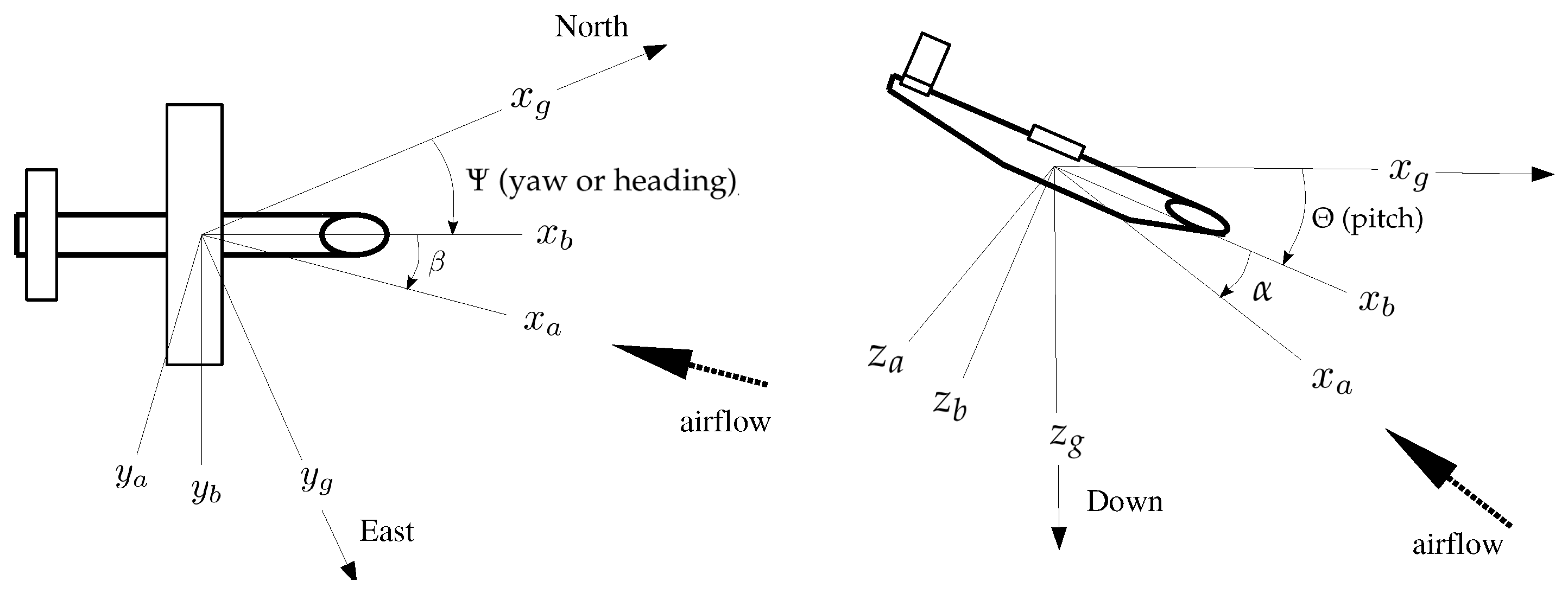
2.1. Wind Vector Measurement with Multi-hole Probes

Following Boiffier [34], and displayed in Figure 1, we use the Earth coordinate system, or geodetic coordinate system (index g). Furthermore, the body-fixed coordinate system of the aircraft (index b) is used. The origin is in the center of gravity of the aircraft; x faces forward, y faces starboard, and z faces downward when flying horizontally with zero angle of attack. Besides, the aerodynamic coordinate system (index a), oriented by the direction of the flow relative to the aircraft, is used. The aerodynamic coordinate system has the same origin than the body-fixed coordinate system and, with the angle of attack α (positive for air flow from below) and side-slip angle β (positive for flow from starboard), the aerodynamic coordinate system can be transformed into the aircraft coordinate system using the transformation T b a . The aerodynamic coordinate system and the body-fixed coordinate system have the same origin, but a misalignment between the multi-hole probe’s orientation and the aircraft cannot be avoided and [20,34,35] causes a small difference between the measured flow angles α ˜ , β ˜ (in the wind tunnel or during the flight experiment) and the actual angle of attack α and side-slip β . It can be shown that α ˜ α and that β ˜ β for small angles of attack [35]. Therefore, this is neglected in this study. The coordinate systems and angles are shown in Figure 1. The wind vector w g is calculated [35] using
w g = v g + T g b u b + Ω b × L
with the true airspeed vector u b in the body-fixed coordinate system of the aircraft, and the transformation matrix T g b into the geodetic coordinate system. The velocity vector v g of the UAS, as well as the Euler angles Φ (roll), Θ (pitch), and Ψ (yaw or heading) are used to determine T g b and are estimated with an INS, consisting of a GNSS receiver, an Inertial Measurement Unit (IMU) and an Extended Kalman Filter (EKF). The vector of angular body rates Ω b and its lever arm L describe the transformation due to the spatial separation between INS and the multi-hole probe and can be (according to Lenschow [36]) neglected since the lever arm L is only a few centimeters in our UAS. With the true airspeed vector u a in the aerodynamic coordinate system, the transformation T b a into body-fixed coordinates and the rotation into geodetic coordinates T g b , Equation (1) can be written as
w g = v g + T g b T b a u a
The true airspeed vector u a in the aerodynamic coordinate system requires intensive calibration of the multi-hole probe. The norm | u a | is calculated with the total air temperature T tot , which is assumed to be adiabatically stagnated on the probe’s tip, and the static pressure p, as well as the dynamic pressure increment q.
| u a | 2 = 2 c p T tot 1 p p + q κ
The quantities p and q are calculated with normalized pressure differences between the pressure holes on the multi-hole probe and the wind-tunnel calibration. The Poisson number is defined by κ = R c p 1 , with R = 287 J kg 1 K 1 being the gas constant for dry air and c p = 1004 J kg 1 K 1 the specific heat of dry air. The true airspeed vector u a must be transformed from the aerodynamic coordinate system into the body-fixed coordinate system using T b a
u b = | u a | 1 + tan 2 α + tan 2 β 1 tan β tan α
using α and β .
With T g b , which consists of three sequential turnings (rolling, pitching and yawing), the coordinate system (see also Figure 1) is transformed from body-fixed into geodetic (index g) coordinates. T 1 ( Φ ) defines rolling about x b , T 2 ( Θ ) defines pitching about y b , and T 3 ( Ψ ) defines yawing about z b .
T g b = T 1 ( Φ ) T 2 ( Θ ) T 3 ( Ψ ) = 1 0 0 0 cos Φ sin Φ 0 sin Φ cos Φ cos Θ 0 sin Θ 0 1 0 sin Θ 0 cos Θ cos Ψ sin Ψ 0 sin Ψ cos Ψ 0 0 0 1
Finally, the wind vector w g can be calculated with Equation (2) and transformed into meteorological coordinates (index m) using the transformation T m g :
w m = T m g w g = 0 1 0 1 0 0 0 0 1 w x w y w z
The vector components of the wind vector in meteorological coordinates w m = ( u , v , w ) are u being positive eastward, v being positive northward, and w positive when facing upwards. The presented data in this study is given in the meteorological coordinate system.

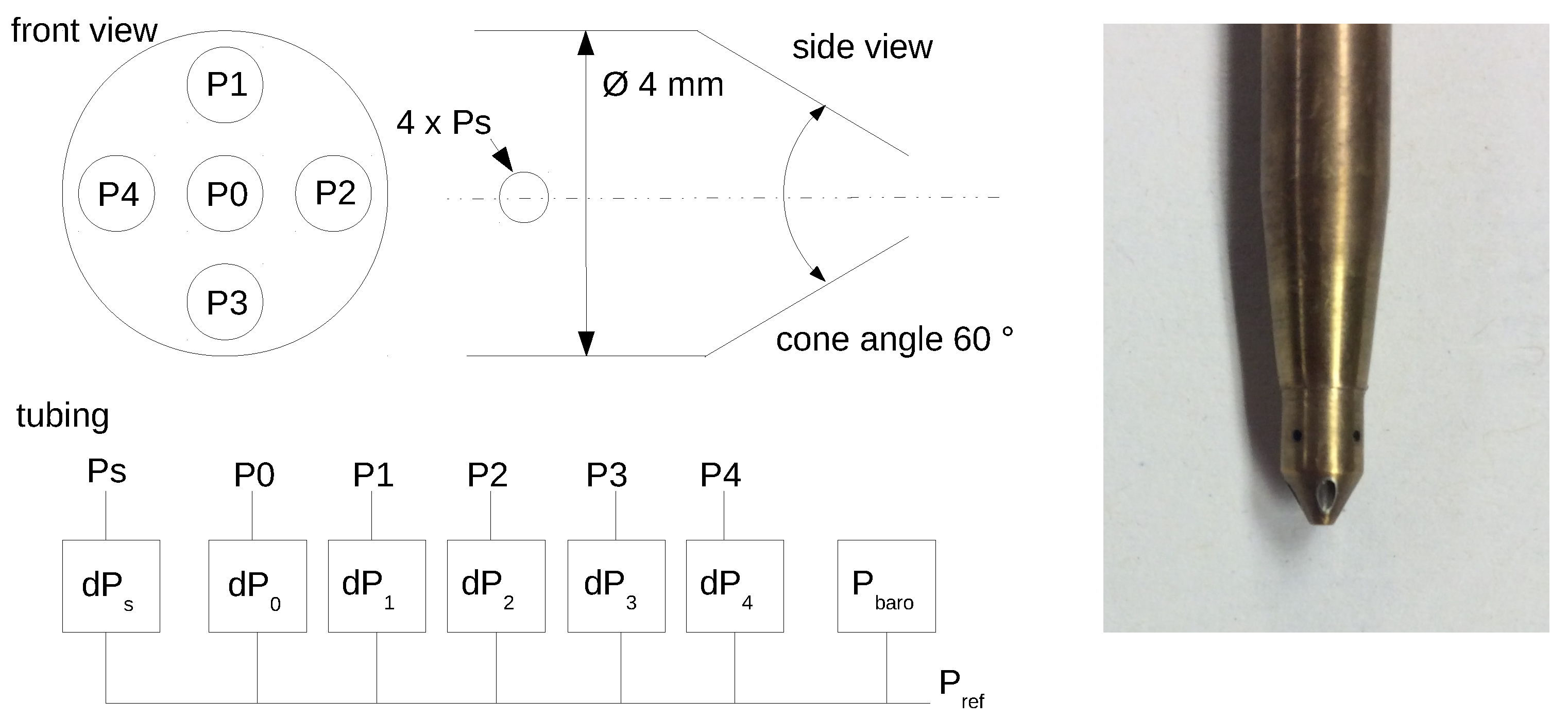
2.2. Five-Hole Probe “Pressures-to-Airflow-Vector”

Generally, there are two fundamental approaches to convert the pressure readings to flow angles, stagnation, and dynamic pressure. Firstly, the pressure field around spherical heads can be described by an analytical model derived with potential theory for fluid dynamics, e.g., as with the BAT probe used by Black et al. [37] or the flow probe used by Metzger et al. [11]. Only spheres or elliptic shapes can be reliably described with this frictionless and incompressible formulation of the flow field with a curl free vector field. Cone tips, on the other hand, are generally fully calibrated in the wind tunnel and the cone angle allows for an adjustment of the angle-sensitivity of the measurement. An overview of relevant geometries and aerodynamic probe design, can be found e.g., in the study of Hall and Povey [38]. MASC uses a five-hole probe (Figure 2) with a tip diameter of 4 mm, a cone angle of ϕ = 60 , forward facing holes and is calibrated from 20 to 20 . The probe, manufactured by the Institute of Fluid Mechanics at the Technische Universität Braunschweig, Germany, follows the following compromise: smaller cone angles or “sharper” tips are more sensitive and the pressure coefficients of the probe react more strongly, if the angle of the inflow tilts. In other words, a small change in the angle of the airflow results in a higher change in the pressure readings, if the probe’s tip is sharp rather than bluff. The downside of sharp probe tips are smaller maximum angles that can be measured and a higher dependency on the Reynolds number. The sensitivity of spheres can be compared with cone angles ϕ > 60 and can be used for flow angles of up to 40 and more. The precision around ± 5 flow angle, where the measurement with UAS and manned aircraft is most important, is worse. Considering turbulence measurements with a fully exploited frequency response of the tubing and the pressure transducers, a tip diameter of 4 mmwas chosen, since the tip diameter should be kept significantly smaller than the smallest eddy that can be resolved [39]. To find a relationship between the measured pressure differences d P i and the airflow angles α and β , as well as the dynamic pressure q and static pressure p at any airflow angle within the calibration range, wind-tunnel calibrations were conducted. Previous efforts to measure the 3D wind vector with a similar five-hole probe were made e.g., by [7] with the Mini Aerial Vehicle (M2AV). The study by Wildmann et al. [6], who were using the MASC, improved the frequency response and accuracy of the probe by using a different tubing between the pressure holes of the five-hole probe and the pressure transducers, and by applying dimensionless calibration coefficients according to Treaster and Yocum [40]. The same setup as by Wildmann et al. [6] is also used in this study and the description of the holes, the dimensions, the schematic tubing and a picture of the probe’s tip are given in Figure 2.
To find a relationship between the measured pressure differences d P i and the airflow angles α , β , as well as q and p, a polynomial fit is applied and dimensionless coefficients [6,40] are defined:
Δ P = ( d P 1 + d P 2 + d P 3 + d P 4 ) 4 q c = 1 2 ρ v c 2 k α = d P 1 d P 3 d P 0 Δ P k β = d P 2 d P 4 d P 0 Δ P k q = d P 0 q c d P 0 Δ P k p = P s + Δ P Δ p c d P 0 Δ P
In the wind tunnel a dynamic pressure q c is set for the calibration and the static pressure p c is recorded. The dimensionless coefficients k α and k β are the variables of the polynomial functions for α , β , k p and k q , whereas k p and k q are correction values for the measurement of q and p with regards to the airflow angle at the probe. The probe, when used as pitot-static tube, would not be independent of the flow angles, since the aerodynamic design of the probe’s tip is unsuitable for that. The aim of the calibration is to find the functions f x ( k α k β ) to calculate α , β , k p and k q from the pressure readings of a flight experiment:
α = f α ( k α , k β ) β = f β ( k α , k β ) k q = f q ( k α , k β ) k p = f p ( k α , k β )
For all the four functions f x , a polynomial fit is selected with a specific set of parameters c x for each function. The functions f x ( k α , k β ) can be determined from the scalar product of the two vectors k ( k α , k β ) and c x
f x ( k α , k β ) = k ( k α , k β ) c x = k α 0 k β 0 , k α 0 k β 1 , , k α 0 k β m , k α 1 k β 0 , , k α m k β m c x , 0 , 0 c x , 0 , 1 c x , 0 , m c x , 1 , 0 c x , m , m ,
whereas c x is a constant parameter vector with, in this case, the parameters for m = 9 and a polynomial of 9th order. The goal of the calibration procedure is to determine the four parameter vectors c α , c β , c q and c p . They are estimated from the calibration data, consisting of the quantities α , β , k α , k β , k q and k p . Both α and β are changed from 20 to 20 , in steps of 2 , resulting in 21 × 21 data points. This leads to an overestimated system of equations that is solved with a least squares method for the unknown parameter vectors c x . The solution c x is the best fit of the least squares method and is used to estimate velocity and flow angles in arbitrary flows by converting the instantaneous pressure measurements at each hole of the probe to instantaneous Δ P , k α , k β according to Equation (7). Subsequently, α , β , k q and k p are calculated with
α = k c α β = k c β k q = k c q k p = k c p
and finally, the static pressure p and the dynamic pressure q are calculated by using Equation (7) and solving for p and q:
p = P s + Δ P k p · d P 0 Δ P q = d P 0 k q · d P 0 Δ P

2.3. Wind-Tunnel Measurements

Since the reference side, or low-pressure side, of the differential pressure transducers for the calibration is well out of the turbulent self-similar round jet [41], there is no difference between the ambient pressure in the facility and the static pressure inside the flow field of the open jet during the calibration. The static pressure difference during the calibration is therefore Δ p c = 0 . The airspeed v c is constant throughout the calibration and continuously monitored with an independent measuring system. The ambient pressure p baro , the airspeed v c , as well as temperature and relative humidity are recorded continuously. The probe head blockage was 0.02 % of the nozzle exit area, which has a diameter of 0.2 m and the calibration is therefore not influenced according to Dominy and Hodson [22]. The calibration apparatus ensures that the probe’s tip is always in the same position for all angle combinations during the calibration. This middle section of the open jet stream was analyzed prior to the calibrations. The turbulence intensity, calculated with a 10 min time series of the central hole d P 0 at α = β = 0 , for v c = 22.5 m s 1 , yields 0.04 % .

2.4. MASC and the Methods for Deriving Mean Values and Turbulence Statistics

The environment-physics group at the Center for Applied Geoscience (ZAG), University of Tübingen, Germany, designed and built the research UAS MASC (see Figure 3). Together with the ground control station for the autopilot and the sensor system, MASC is classified as UAS. MASC [6] is an electrically propelled single-engine (pusher) aircraft of 4 m wing span and weighs about 6 kg, including 1 kg scientific payload. Height, flight path and all other parameters of flight guidance are controlled by the autopilot system PixHawk 2.1. The scientific payload consists of several subsystems to measure the 3D wind vector, air temperature and water vapor, including a fast thermometer (fine wires, see [42]), a five-hole flow probe [7,39] and an INS called Ellipse2-N by SBG-systems.
All sensors are sampled at 100 Hz and measure atmospheric turbulence. Considering the individual sensor inertia, a final resolution of about 30 Hz is achieved and thus, small turbulent fluctuations are resolved, while the Nyquist theorem is fulfilled. Typical flight patterns with MASC (these are common flight strategies for any research aircraft) are horizontal straight and level flights (so-called legs) both at constant height or stacked at various flight levels. These flight legs are used to calculate turbulence statistics and turbulent fluxes (e.g., [43,44]), spectra, mean values but also the influence of surface heterogeneity and orography on the lower atmosphere. Two consecutive straight legs including the turns (a full round) are referred to as racetrack. The probe (five-hole probe, see Figure 2 and Figure 3) in use with MASC operates normally at 22.5 m s 1 and the Reynolds number in an International Standard Atmosphere (ISA) is Re = 6.04 × 10 3 , calculated with
Re = | u a | ρ d μ ,
using the norm of the true airspeed vector | u a | , the density ρ and the dynamic viscosity μ of the air and the characteristic length d, being the tip diameter of the probe. The desired margin for the probe in the setup with MASC, ranges from 15 m s 1 until 30 m s 1 cruising speed, under polar condition with 20 C until 40 C, and from sea level pressure of 1013 hPa until high altitude flights and low ambient pressure. The desired range can be from Re 10.41 × 10 3 at 30 m s 1 true airspeed, 20 C and sea level pressure and Reynolds numbers as low as Re 2.50 × 10 3 on a hot summer day in high altitudes and low airspeed. In this context, it is important to consider the behavior of the PixHawk 2.1 flight controller, which controls the indicated airspeed during the measurement. The indicated airspeed (IAS) is measured with a pressure transducer and the influence of the density of the air is not considered. As a rule of thumb, the true airspeed equals the IAS under ISA conditions, and with increasing altitude, round about every 300 m, the true airspeed is 2% higher than IAS. The actual true airspeed is calculated in the post-processing and may vary significantly if the altitude changes during the experiment. The Reynolds number cascade measured in the study of Dominy and Hodson [22] ranges from 4 × 10 3 < Re < 500 × 10 3 and identifies formally the effects of flow separation from the body of the probe or from the leading edge. Especially for the lower Reynolds numbers towards Re = 4 × 10 3 , flow separation becomes sensitive and it has been demonstrated that artificial turbulence in the wind-tunnel influences the measurement generally for Re < 20 × 10 3 .
Three flights were chosen for this study. The first flight experiment (in the following referred to as ISOBAR) was conducted during the ISOBAR campaign, which was described by Kral et al. [33], presenting the numerous measurement systems of the campaign. The second flight (in the following referred to as COMPLEX) was conducted in complex terrain near Schnittlingen on the Swabian Alp in the South of Germany. This flight was also used by the study of Wildmann et al. [24], who investigated the flow field in the vicinity of the apparent test field for wind energy. The third flight experiment (in the following referred to as WAKE) is one transect through the wake of a wind turbine near Wilhemshaven in the North of Germany. The flights ISOBAR and COMPLEX were chosen to analyze the influence of airspeed variations on mean and turbulence quantities. The basis for all these quantities is the straight level flights (legs), where the turns are cut off. The mean values for temperature, windspeed, and direction are directly calculated from the time series of each flight leg. To analyze the influence on the turbulence measurement, the turbulent kinetic energy TKE, the variance of the vertical wind component Var(w), the covariance of the vertical and horizontal wind components Cov( w , u ) and Cov( w , v ) and the integral length scale of the vertical L ( w ) and horizontal wind L ( v h ) are calculated, since these are dependent on the calibration of the probe and the most important quantities for ABL studies. The third flight WAKE was chosen, because large changes in airspeed occur during the transect through the wake of the wind turbine, and to show the instantaneous effect of the calibration of the five-hole probe on features in the wind field. The high-resolution data is plotted as a time series to analyze the deviations and uncertainties if the airspeed of the measurement does not fit the airspeed of the calibration. Along with the windspeed and direction, also the calculated angle of attack α and side-slip angle β are analyzed together with data from the INS, showing the motion of the UAS during the transect through the wake of the wind turbine.
The horizontal windspeed v h is calculated with the wind vector components u and v by
v h = u 2 + v 2 .
The variance of a variable X is calculated, using Reynolds decomposition where the fluctuations X are separated from the mean X ¯ , with
Var ( X ) = 1 N 1 i = 1 N ( X i X ¯ ) 2 = X ¯ 2 ,
where N is the number of data points and X ¯ denotes the average of the variable within the data window or, in this case, within the individual flight leg. The covariance Cov( X , Y ) of two variables is calculated respectively by
Cov ( X , Y ) = 1 N 1 i = 1 N ( X i X ¯ ) ( Y i Y ¯ ) .
The turbulent kinetic energy TKE is calculated with the velocity fluctuations (variances) Var(u), Var(v) and Var(w) of the wind vector components
TKE = 1 2 Var ( u ) + Var ( v ) + Var ( w )
and equals the turbulent normal stress. The integral length scale L [35,45,46,47] is calculated by multiplying the integral time scale I with the mean true airspeed of the flight leg. The integral time scale I ( v h ) of, for instance, the horizontal windspeed v h is defined by
I ( v h ) = 0 τ 1 δ τ v h ¯ ( t + τ ) v h ¯ ( t ) v h ¯ 2
and multiplied by the mean true airspeed | u a ¯ |
L ( v h ) = I ( v h ) | u a ¯ |
to get the integral length scale L ( v h ) . The integral time scale I is the autocorrelation function of the variable and calculated by integration from zero lag to the first crossing with zero at τ 1 [47]. The integral length scale of the vertical wind vector component L ( w ) is calculated respectively, with I ( w ) multiplied by | u a ¯ | . The integral length scale can be interpreted as the typical size of the largest, or most energy-transporting eddy.

3. Results and Discussion

Firstly, this study investigates the magnitude of deviations of mean values and turbulence quantities, when measuring with a calibration that does not exactly match the airspeed during the experiment. To some extent this is not avoidable, since turbulence and non-stationary flow causes the UAS to accelerate and decelerate due to its momentum, drag, and the flight-mechanical properties. To evaluate that, the deviations when calculating mean values and the deviations when calculating turbulent quantities must be considered. It is impossible to setup an experimental study in the wind tunnel, since atmospheric turbulence cannot be artificially produced in a representative way. Qualitative studies in the wind tunnel, where the turbulence intensity increased consecutively, showed that the flow separation on the probe’s tip is influenced, especially for Re < 20 × 10 3 [22].
The second main issue of this study is the desired flexibility for the cruising airspeed of the autopilot and a procedure to compensate for deviations between the airspeed of the calibration and the flight experiment.

3.1. Polynomials at Different Reynolds Numbers

To investigate the deviations when calculating mean values from calibrations at different airspeeds, the data from the wind tunnel is already giving insight. In Figure 4, the results of three calibrations in the wind tunnel are presented. The polynomials were recorded at airspeeds of v c 1 = 15 m s 1 , v c 2 = 22.5 m s 1 and v c 3 = 28 m s 1 , yielding, with the apparent ambient pressure, temperature and humidity in the wind-tunnel facility, Reynolds numbers at the probe’s tip of Re v 1 = 3695 , Re v 2 = 5538 and Re v 3 = 7031 . The high speed v c 3 is the maximum for the used sensor system, because the maximum differential pressure of the front hole is 500 Pa. The low airspeed of v c 1 = 15 m s 1 was chosen to mark the lowest expected airspeed of the measurement, since the cruising airspeed of MASC can be set as low as ≈18 m s 1 and during turbulence the airspeed can reduce further. The plots show the 21 × 21 dimensionless coefficients k α , k β plotted for α and β in steps of 2 from 20 to 20 . The comparison in Figure 4 already reveals how important a consideration in this margin of Reynolds numbers is. Especially for angles ≥±10 the differences are obvious. Since the calibration map for Re v 1 = 3695 is uniform and almost linear throughout the whole span from 20 to 20 , the sensitivity throughout the whole domain is nearly constant, yielding that this airspeed is better for the measurement, than higher airspeeds. The polynomials of Re v 2 = 5538 and Re v 3 = 7031 become skewed and therefore less sensitive for higher α and β . This means that a change in α and β of e.g., 2 corresponds to a smaller change in the pressure readings. The map of k α and k β is best in terms of precision, if it spans a wide grid and if it is uniform throughout the domain of definition.
Figure 5 shows an evaluation of the coefficients k q and k p . As an example, the coefficients are plotted over β , ranging from 20 to 20 . Three constant angles of attack α = 10 , α = 0 and α = 20 are chosen to show the behavior of k q and k p for the three calibrations.
The following behavior of k q at v c 1 , v c 2 and v c 3 is stated:
  • The dynamic pressure coefficients k q for v c 2 and v c 3 are close together, but k q for v c 1 lies below and has a larger offset.
For α = 0 the dynamic pressure coefficients k q for v c 2 and v c 3 are close together, but for v c 1 at α = 0 and α = 10 , the difference is significant. For α = 0 all three curves generally vary little over the considered range of β and for all three calibration speeds. The magnitude of k q at v c 1 varies the least over range of β compared to v c 2 and v c 3 at α = 0 and α = 10 . The varying generally increases for α = 10 and again for α = 20 , revealing the necessity of the calibration of the dynamic measurement. It is remarkable how strong the changes of k q for v c 2 and v c 3 are between α = 10 / α = 0 and the biggest angle α = 20 , because the level of k q drops significantly for v c 2 and v c 3 and the curve of v c 3 even lies below v c 2 for α = 20 . The curves of k q for α = 20 , drop to significantly to smaller values for v c 2 and v c 3 , because the structure of the flow separation on the probe’s tip behaves differently between v c 2 / v c 3 and v c 1 . This is also visible for k p .
  • A characteristic local minimum persists around β = 0 for α = 0 and for all three curves of k q . This feature varies for the individual parameters.
For α = 0 , a characteristic drop of k q between 10 β 10 , where a local minimum persists at β = 0 , is also showing a dependency on the calibration speed. This feature is pronounced for v c 1 , significantly weaker for v c 2 and not apparent for v c 3 . For α = 10 , α = 0 and α = 20 , the curves of k q show a similar behavior for the range of β when inter-compared, although the local minimum at β = 0 does not exist for α = 10 and α = 20 .
  • It is concluded that the polynomials of k q and k p for v c 1 is the most robust for tilted flow, since the curves for v c 2 and v c 3 have a stronger gradient between α / β 10 and α / β 10 .
The curves of the static pressure coefficients k p , when compared between the three angles of attack α , change their characteristics in a similar way for all three calibration speeds, except for α = 10 and v c 1 . Here, the flow separation on the probe’s tip behaves differently. For α = 20 , the curves of k p for v c 1 and v c 2 have a local minimum at β = 0 , but v c 3 does not. Generally, the static pressure measurement is the most sensitive compared to k q and the measurement of α and β themselves in tilted flow [6] and when looking at Figure 5 it becomes clear that the dependency on the Reynolds number is also very high. Generally, the static pressure is an elaborated task, since many influencing factors disturb the measurements [48] and only trailing cones can reliably measure the undisturbed static pressure from an aircraft. Therefore, further evaluation considering the true static pressure estimation is not made in this study.
The best calibration polynomials can be calculated from the calibration at v c 1 , since k q and k p in Figure 5, and also k α and k β in Figure 4, are the most uniform throughout the domain of definition. The enhanced skewness of k β over k α in Figure 4, for v c 2 and v c 3 , leads to more skewed polynomials for k q and k p . It is concluded that the calibration reacts strongly to changes of the Reynolds number for both k q and k p , as well as for k α and k β . Section 3.4 discusses the application of the interpolation between polynomials to increase the precision, and the use of an independent pitot-static tube is suggested. Doing so, the determination of the true airspeed and the static pressure with the five-hole probe becomes obsolete, since a pitot-static tube can measure theses quantities more reliable in tilted flow and for varying Reynolds numbers and with almost no calibration effort.

3.2. In-Flight Calibration of the Wind Measurement

The aerodynamic coordinate system and the body-fixed coordinate system have the same origin, but a misalignment between the multi-hole probe’s orientation and the aircraft cannot be avoided, and a correction must be applied. Therefore, three offset corrections for Φ (roll), Θ (pitch), and Ψ (yaw or heading) must be determined. A forth correction factor f t a s for the norm of the true airspeed vector | u a | must be determined to account for the calibration in the wind tunnel, which never matches exactly the conditions during the measurements, since the calibration of the whole UAS including the engine etc. is not feasible and especially because the reference side of the pressure transducers have the ambient pressure of the wind-tunnel facility as reference during the calibration, and because in-flight, the pressure inside the fuselage is the reference for the pressure transducers. The procedure to calculate the correction factors was explained in detail by Van den Kroonenberg et al. [7]. The assumption for the in-flight calibration are a constant mean horizontal wind, a mean vertical wind near zero and low turbulence or turbulent transport. This allows a comparison of the wind components for two consecutive straights in opposite directions (star pattern), or identical legs in reverse direction. This procedure yields the correction offset Δ Ψ for the yaw angle, Δ Θ for the pitch angle and the correction factor f t a s for the norm of the true airspeed | u a | . The offset Δ Φ for the roll angle is set to zero and can be, according to Van den Kroonenberg et al. [7], neglected, since the influence on the wind components is very small. The offsets Δ Ψ and Δ Θ are applied to the transformation T g b in Equation (5) and the factor f t a s is multiplied with the norm of the true airspeed vector | u a | in Equation (4). To ensure comparability between the three calibrations, the correction offsets and factors are determined in the exact same way. Meeting the assumptions of constant wind and zero vertical wind is always a delicate task. For the flights ISOBAR and COMPLEX, the three pairs of consecutive legs on the highest flight level were chosen to calculate the correction offsets and factors. The average of those was calculated and applied to the whole flight. The results for the three calibration polynomials are written in Table 1. The WAKE flight uses fractions of two consecutive racetracks on 125 m AGL that were not disturbed by the wake of the turbine. These fractions of the legs represent the free stream, passing the wind turbine. The averages of two pairs were taken and the results are also written in Table 1.
Table 1 shows that the offsets Δ Ψ and Δ Θ are in the same range for all applied calibrations and vary ≈1–6 between the flights. This is mainly due to the previously described misalignment of the probe and the UAS. The correction factors f t a s for the true airspeed vary systematically for the three calibrations, since the values smaller than 1 were calculated for the calibration speeds v c 1 for all experiments, causing a reduction of the true airspeed. The values of f t a s for v c 2 are slightly bigger, or equal to 1, and the values for v c 3 are again higher. This is expected, since k q in Figure 5 is significantly lower for v c 1 and the actual true airspeed of the measurement was set to 22.5 m s 1 for the autopilot. The results for the correction factors f t a s for v c 2 and v c 3 follow the same logic, but differ less significant, since the curves for k q in Figure 5 are also closer together. The level of the three correction factors f t a s when inter-compared between the experiments also differs, which is mainly caused by the thermodynamic differences, or differences in the density of the air, and by the airspeed setting of the autopilot, which is also affected by that, and generally not precisely calibrated. The actually measured true airspeeds during the individual flight experiments, as well as an overview of the persisting meteorological conditions, are written in the Table 2, Table 3 and Table 4.
Two things are very important to be noted here. All correction factors do influence each other to some extent and are not independent, but since they are all derived in the exact same way, the comparison in terms of deviations between the calibrations is not affected by that. On the other hand, it cannot be stated that there were no general offsets caused by the correction factors. This remains as an uncertainty and is subject to the overall conclusion and recommendations for future measurements.

3.3. Flight Experiments: Influence of Different Calibration Speeds on Mean Values, Turbulence Statistics and Single Flow Features

Three different polynomials are applied to data of three flights in different atmospheric conditions to be able to argue the influence of airspeed variations of the UAS during the measurements. Firstly, the ISOBAR flight with low atmospheric turbulence is shown in the Figure 6, Figure 7, Figure 8 and Figure 9 and compared to the COMPLEX flight in the Figure 10, Figure 11, Figure 12 and Figure 13 with high turbulence in complex terrain. Every data point consists of one headwind leg. To evaluate the persistent condition of these two flights, the set of plots in the Figure 6, Figure 7, Figure 8, Figure 9, Figure 10, Figure 11, Figure 12 and Figure 13 consist in the subplot on the left-hand side, of height profiles of the quantities that are calculated with the polynomial at v c 2 . The deviations are given in the subplot on the right-hand side, where the red ( v c 1 ) and blue ( v c 3 ) bars display the absolute deviations of the quantity to the value, calculated with the polynomial at v c 2 .
To show the influence of a big and sudden change in airspeed, when passing through tip vortices and the windspeed deficit of the wind turbine, the WAKE flight is analyzed in the Figure 14, Figure 15, Figure 16 and Figure 17. The time series of the whole transect for several quantities of the measurement system is given in Figure 15, and a zoom into the first passage in the vicinity of a tip vortex, is given in the Figure 16 and Figure 17.

3.3.1. Low Turbulence in Stably Stratified Nocturnal Polar Boundary Layer (ISOBAR)

The ISOBAR flight was conducted in the north of the Bothnian Bay in Finland on the 21 February 2017 between 05:01 and 05:48 UTC, which is 07:01 a.m. local time. The intensive measurement campaign was described by Kral et al. [33]. MASC was operated in the dark and started on the lowest flight level of 25 m AMSL and ascended afterwards in steps of 25 m to 150 m AMSL, followed by steps of 50 m. The lower surface layer is sampled denser to capture the ground-based inversion. The orientation of the racetracks and the flight direction of the legs, contained in the set of plots, was about 350 to be oriented against the mean wind direction. The data only consist of the headwind legs, since the fetch, when flying headwind, differs significantly from the tailwind legs. The length of the legs is about 1200 m. An overview of the conditions during the ISOBAR flight is given in Table 2. The stably stratified surface layer was about 75 to 100 m thick, as indicated by the profiles of potential temperature, windspeed and direction in Figure 6. The windspeed was ≈6 m s 1 on the lowest level and ≈9.5 m s 1 above the ground-based inversion quite high and the wind direction turned from ≈325 to ≈365 on 275 m AMSL. The profile of the wind direction indicates another slightly different regime above 125 m AMSL and again, visible in the profile of potential temperature and windspeed, a layer above 250 m AMSL.
The deviations when using the calibrations at v c 1 and v c 3 , which do not fit the actual airspeed of the measurement, reveal their influence on the calculation of mean values. Generally, the influence on windspeed and direction, averaged over the whole leg, can be rated as small. The maximum deviation is 0.2 m s 1 and 0.4 . Supported by the investigations of other flights during this campaign, no trend or significant correlation with other parameters was found for the absolute deviations of the mean values. Furthermore, also relative deviations do not show any trend or correlation for the deviations of the mean values. The actual averaged true airspeed, calculated with the polynomial at v c 2 = 22.5 m s 1 for the ISOBAR flight was, averaged over all flight levels, | u a ¯ | = 24.46 m s 1 . The highest standard deviation was measured on the lowest level with | u a ¯ | = 24.18 ± 0.31 m s 1 . The highest true airspeed of the whole ISOBAR flight was | u a | = 25.53 m s 1 and the lowest true airspeed was | u a | = 22.98 m s 1 . Although the autopilot was set to 22.5 m s 1 , the post-processing revealed a higher true airspeed.
The profiles of TKE and the Var(w) in Figure 7 show a uniform distribution for the SBL, where turbulence is suppressed. With the persisting wind direction, the air mass had a fetch of at least 50 km over the frozen Bothnian Bay, which is homogeneous terrain that cools the air above it. The surface layer forms due to friction, and TKE and Var(w) increase towards the ground. Another source of turbulence is the top of the surface inversion, where the geostrophic wind causes shear between the layers. This is also reflected in the measurements, since the TKE on 125 and 150 m AMSL is increased and the Var(w) too, although little. Here, the deviations when applying the calibration at v c 1 and v c 3 do have a clear trend. Higher turbulence towards the ground causes higher deviations, but a constant relative deviation does not exist. The relative deviations vary randomly between almost 0% and up to 20%.
The covariances Cov( w , u ) and Cov( w , v ) in Figure 8 are used to estimate the turbulent momentum flux and are also directly influenced by the calibration of the five-hole probe. The values between 75 and 250 m AMSL are close to zero, indicating that there was no significant vertical flux of momentum. On the highest flight level, the temperature and windspeed profiles indicate a change of the wind field, which is also visible in the profile of covariances. In the surface layer, a negative momentum flux towards the surface is expected. The lowest leg on ≈25 m AMSL gives a negative flux, but the next flight level has a slightly positive flux and is already influenced by the shear above the surface-based inversion [49]. Certainly, one would have to transform the coordinate system into the main wind direction for further analysis. The resolution in the surface layer is unfortunately too small to be able to give sufficient insight into the momentum flux, but it is remarkable that MASC can measure consistently small values close to zero without outliers. The deviations of the covariances are generally high and especially for the two height levels above the ground. The peak value for Cov( w , u ) on the lowest flight level has relative deviations of 30% and 35% and for the covariance Cov( w , v ) on 54 m AMSL, the relative deviation is almost 100%. This time, the deviations, when using the calibration at v c 3 , do result in a higher deviation, than using the calibration at v c 1 . This is not the case for the other parameters. There was no reason found for that and the amount of data is not sufficient to draw further conclusions.
The integral length scale L is an important criterion to judge, whether the time series and the fetch of the measurement was long enough to measure turbulence representatively, and to estimate turbulent fluxes [50]. Besides, the statistical error can be calculated according to Mann and Lenschow [51]. The L was calculated for the vertical and the horizontal wind in Figure 9. The profile of L ( v h ) reflects the previously described structure of the ABL, according to the turbulence regimes in the different layers. The turbulence regime in the surface layer has a strong gradient but is poorly resolved. The layer above, driven by shear, inherits the biggest structures for the horizontal wind components, and in the third turbulence regime towards the highest flight levels, L ( v h ) increases again. Here, also L ( w ) increases. With a length of the legs of about 1200 m and a maximum L of 75 m, the biggest eddies of the flow are sampled at least 15 times. The L ( w ) , in general, is small, since the ABL is stably and neutrally stratified. On the one hand, the deviations of L ( v h ) are slightly higher if the actual values are high. However, no trend for the absolute or relative deviation, either towards the calibration at v c 1 nor the calibration at v c 3 can be identified. Although the turbulent kinetic energy and the variance of the vertical wind on the lowest level is increased, the deviations of the L on the lowest level are not. This is another indication that airspeed variations must be considered and that the calibration of the probe is of major importance for the turbulence statistics, since the random nature of turbulence does not allow for simplifications, causing high uncertainties. Unavoidable airspeed fluctuations during the measurement do influence the turbulence measurements, and significant offsets between the airspeed of the measurement and the airspeed of the calibration must be considered. The influence for turbulence statistics is significantly higher than for mean values.

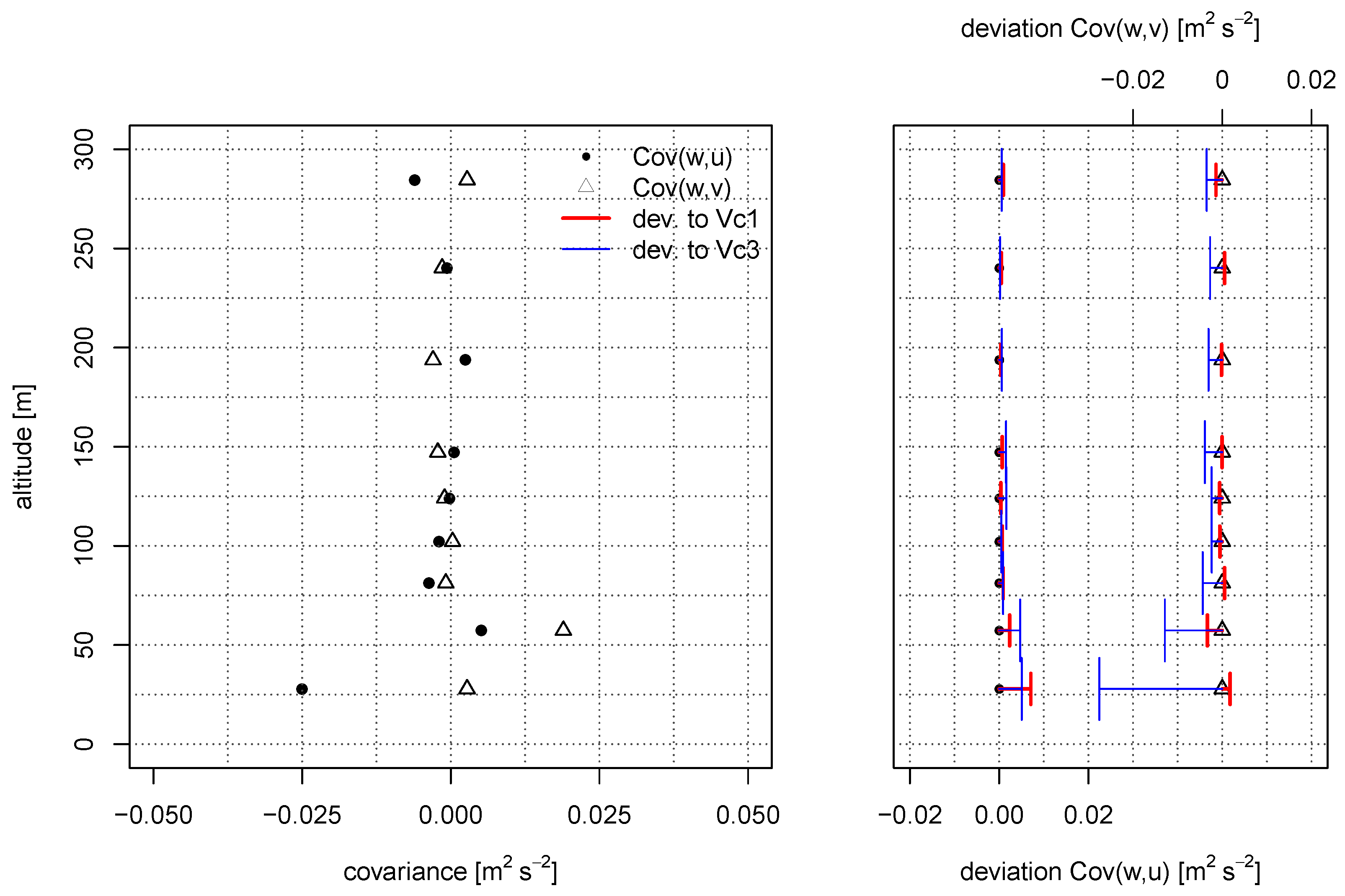
3.3.2. High Turbulence in Complex Terrain (COMPLEX)

The mission of the COMPLEX flight was the investigation of a test site for wind energy in complex terrain. The test site is located on the Swabian Alb, in the South of Germany, near Geislingen an der Steige. The plateau, where the potential site for wind turbines is located, is about 200 m elevated from the valley and in the vicinity of a crest (or escarpment) that is located westerly. The study of Wildmann et al. [24] investigates the flow field using MASC and the studies of Knaus et al. [52] and Schulz et al. [53] compare MASC measurements with numerical simulations, LiDAR and meteorological tower measurements. The COMPLEX flight in this study was conducted in the afternoon of the 27 March 2015 between 13:02 and 13:46 UTC in convective conditions with cumulus overclouding, westerly wind directions and 8 to 9 m s 1 mean windspeed. The ISOBAR flight in Figure 6 and the COMPLEX flight in Figure 10 were chosen, because the windspeed has about the same magnitude, making this comparison significant when analyzing the substantially different turbulence regimes of these flights. This flight is one of the 18 flights of the study by Wildmann et al. [24] and was also used in the comparisons [52,53]. The wind field in these conditions is strongly influenced by the crest, which is overflown forth and back with an orientation of the flight path of ≈285 for the headwind legs. The lowest flight level is 75 m above the take-off position on the plateau of the Swabian Alp, which corresponds to about 790 m AMSL. After the lowest level, MASC ascended in steps of 25 m to 1015 m. The length of the legs is about 1000 m. In dissociation of the study of Wildmann et al. [24], investigating the wind field, in this manuscript, the mean values and turbulence statistics are calculated from the whole leg. To study the wind field, Wildmann et al. [24] split up the legs into certain windows, but for the analysis of deviations due to airspeed variations, the total length of the time series is used for the calculations. The length of each leg was about 1000 m and, to foreclose argumentation concerning the turbulence statistics, with an L of up to 200 m, the turbulent flux of momentum cannot be calculated representatively with a single leg. In this wind field, essentially influenced by the crest, it is more explicit to interpret the covariances as the off-diagonal components of the Reynolds stress tensor and the variances of the wind components as the diagonal components [41]. Standard ABL profiles cannot be expected. Previous studies showed Wildmann et al. [24], Knaus et al. [52] that normalization and averaging with several flights in similar conditions, yields representative local features of the wind field, by averaging out transient flow features and convection. Nevertheless, to argue the deviations when applying different calibrations of the five-hole probe, the turbulent conditions are insightful and in comparison with the rather calm conditions of the ISOBAR flight, the influence of airspeed variations becomes distinct.
An overview of the conditions during the COMPLEX flight is given in Table 3. The potential temperature profile in Figure 10 indicates a convective ABL with a step of 0.4 C between the forth and fifths height level. While the windspeed profile is relatively uniform, the profile of wind direction has also high gradients between 870 m and 915 m AMSL. Intensive shear, and the separation between two regimes persists. The lower layer is strongly influenced by upstream features of the orography and the crest itself. Despite strong turbulence, the deviations for mean values are, with a maximum of 0.1 m s 1 and 0.2 , small and in the same order of magnitude as for the ISOBAR flight. The actual averaged true airspeed, calculated with the polynomial at v c 2 = 22.5 m s 1 for the COMPLEX flight was, averaged over all flight levels, | u a ¯ | = 24.13 m s 1 . The highest standard deviation was measured on 915 m AMSL with | u a ¯ | = 24.21 ± 1.14 m s 1 . The highest true airspeed of the whole COMPLEX flight was | u a | = 28.59 m s 1 and the lowest true airspeed was | u a | = 20.14 m s 1 . The variations of the true airspeed are significantly higher than for the ISOBAR flight.
The turbulent kinetic energy TKE and the variance of the vertical wind component Var(w) is, with more than 3 m 2 s 2 , higher than for the ISOBAR flight by a factor of 30. The two turbulence regimes above and below 915 m AMSL are clearly visible in Figure 11, since below the values spread around ≈2.2 m 2 s 2 and above around ≈0.8 m 2 s 2 . The deviations are higher, if the persistent TKE is higher, but the relative deviations are, with a maximum of 4.2%, very small compared to the ISOBAR flight. The deviations when using the calibration at v c 3 and at v c 1 give randomly higher and smaller values for the TKE, whereas the deviations for the variance Var(w) are uniformly distributed with higher values for the polynomial at v c 3 and lower values for the polynomial at v c 1 . The covariances Cov( w , u ) and Cov( w , v ) in Figure 12 are, with up to 0.75 m 2 s 2 , by a factor of 30 higher than for the ISOBAR flight. At a first glance, one would expect an upward transport of momentum due to the upwind, caused by the crest. This is true, if fractions, or windows of the legs that represent specifically the footprint of the crest are analyzed. Since only less than a third of the legs inherit an up-draft, and the downstream part of the wind field re-attenuates to the plateau, the mean direction of the momentum in the lower five flight levels is oriented downwards. Above 925 m AMSL, in the upper persistent layer, the stresses are closer to zero. In dissociation to the turbulent kinetic energy and the variance of the vertical wind component, the covariances depend strongly on the calibration of the five-hole probe. With relative deviations of more than 100% it is delicate, in terms of airspeed variations, to measure reliably covariances in high turbulence. It is interesting to see that the deviations for TKE and Var(w) do not scale with the magnitude of the value, since the ISOBAR flight in low turbulence shows deviations of up to 20% and the COMPLEX flight in very high turbulence, only a maximum of 4%. The deviations of the covariances, on the other hand, do scale with the actual value and are, by a factor of ten, higher than for the ISOBAR flight. It is concluded that airspeed variations cause disproportionately high deviations for these statistical moments of second order, since the covariances are calculated from the turbulent part of two quantities.
The plot of L in Figure 13 inherits also the two layers below and above 925 m AMS, with very small values for L ( w ) on the two lowest levels, where also the deviations of those are very small. The reason is that close to the ground, the scales of the vertical wind are small and cannot grow due to the surface underneath. The L ( v h ) is, with ≈100 m, quite constant in the lower layer and varies more in the higher layer. This is inversely correlated with the TKE and the Var(w) which is also the case for the ISOBAR flight in the highest two legs. While the influence of the surface decreases, patterns of the geostrophic wind become dominant, shifting the spectrum of the turbulent features towards bigger structures. The influence of the calibration polynomials at v c 3 and v c 1 in the right-hand subplot of Figure 13 are asymmetric. The calibration at v c 1 deviates more than the calibration at v c 3 , both for L ( v h ) and L ( w ) , whereas the opposite behavior occurs for the covariances. The ISOBAR flight does not show this behavior. There was no explanation found for that and it is concluded that airspeed variations must be considered, especially for the calculation of covariances and integral length scales.
To some extent, the absolute deviations of all turbulence quantities show a trend, since high values cause higher deviations and vice versa. For the ISOBAR flight this is also indicated, but less obvious. The trend for the absolute deviations is overlain by the random nature of turbulence and relative deviations do neither have a trend, nor do absolute and relative deviations correlate with each other. Therefore, airspeed variations, or variations of the Reynolds number on the probe’s tip during the measurement, clearly randomly influence the result. The airspeed of the calibration of the probe is of major importance, especially for statistical moments of second order and particularly for covariances and integral length scales of wind vector components.

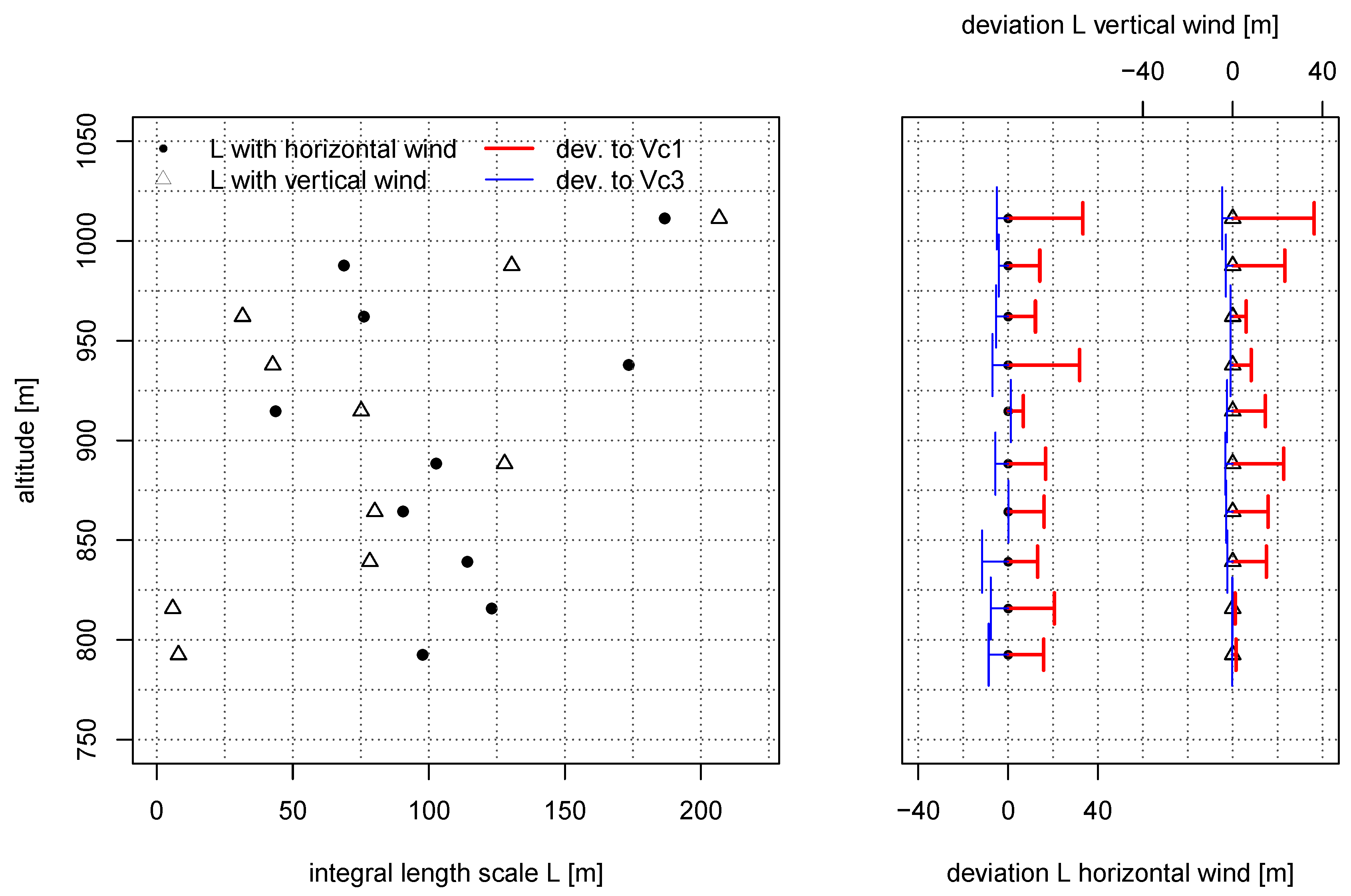
3.3.3. Transect of the Wake of a Wind Turbine (WAKE)

The third flight was performed to study the wind field around wind-energy converters (WEC). In the North of Germany, near Wilhelmshaven, the flow in the vicinity of an Enercon E-112 prototype turbine in the Jade Wind Park, close to the shore line of the German Ocean, was investigated. The helical hose of detaching tip vortices, growing and decaying gradually downstream the WEC, are of great interest, since numerical models show high uncertainties. However, field measurements of small-scale features of the wake and especially the tip vortex helix do not exist and MASC provides unique possibilities to sample in situ measurements of the small scales. A big uncertainty in models is the evolution of the tip vortex helix and decay-rates of the vortices in different atmospheric conditions. To be able to study these processes and validate numerical models, the uncertainties of the wind measurement must be analyzed precisely, since a transect through a tip vortex causes very high gradients of the wind vector components, involving sudden changes in airspeed and attitude of the UAS. The strategy to encounter the tip vortex is shown in Figure 14, where the wake is crossed perpendicular to the mean flow from west to east. Dependent on the position relative to the WEC, the expected size, strength, and orientation of the tip vortices differ and coming along with, the chances to fly through or pass by a vortex.
To analyze the influence of airspeed variations, a transect on hub-height with a distance of one rotor diameter (1D) was chosen. The hub-height of the Enercon E-112 prototype WEC is 125 m AGL and the rotor diameter is 100 m. Figure 14 shows the flight path of MASC with the horizontal windspeed v h in the color code for a transect from west to east. The data is downscaled to 5 Hz. The displayed WEC is only a schematic model and does not have exact dimensions. The yaw angle of the WEC during the measurement is indicated by the 3D model. The wind direction and speed was about 25 and 9 m s 1 for the leg on hub-height and in front of the WEC. The windspeed deficit is clearly visible in Figure 14 and the tip vortices can be identified.
Moreover, Figure 14 shows the schematic orientation of detaching tip vortices of a turbine blade, when considering the cross-section of a horizontal plane on hub-height. Here, it can be assumed that the cross-section of the vortex lies untilted (flat) in a horizontal plane through the center of the rotor. The measurement for this example is located 1D behind the WEC. Assuming that there is no deflection of the wake and the helix of vortices in any direction, the orientation of the vortex at 1D behind the WEC would be the same. The arrows indicate the position of the vortices that were encountered or passed with the flight leg. Assuming incompressible and divergence free flow, a vortex can be described by potential theory, where the velocity field is a simple function of the radius r of the vortex and the circulation Γ , which is the strength of the vortex. This is the basis for simple formulations to describe e.g., aircraft wake vortices [54]. If a tip vortex were traversed through the center, the tangential velocity would increase to its maximum at the core radius r = r c , and decrease to zero, when passing the center at r = 0 , followed by another increase in the opposing direction to its second maximum at r = r c again. During the approach and after the vortex, outside r c , the tangential velocity increases and decreases until the mean flow dominates. This simplification is the basis argumentation for the analysis at which position the vortex was encountered in this study. Further definitions and criteria for vortices are given by Jeong and Hussain [55].
An overview of the conditions during the WAKE flight is given in Table 4. The wind vector components u , v and w, along with the horizontal windspeed and wind direction, the flow angles onto the FHP α and β , the true airspeed | u a | , the heading Ψ and the ground speed in east-west direction v g , e w are plotted as a time series in Figure 15. The time series is the same data as in the Google Earth pictures in Figure 14 and shows the windspeed deficit of the wake. The true airspeed and all data in Figure 15 is calculated with the polynomial of v c 2 = 22.5 m s 1 , which is off the actual airspeed, set for the autopilot. The averaged true airspeed and the standard deviation, calculated with the polynomial at v c 2 = 22.5 m s 1 for the WAKE flight leg, was | u a ¯ | = 18.23 ± 0.76 m s 1 . The highest true airspeed of the WAKE flight leg was | u a | = 20.45 m s 1 and the lowest was | u a | = 16.13 m s 1 . The autopilot was set to 19 m s 1 to be able to sample with a higher resolution in the wake of the WEC.
Prior to the drop in the windspeed deficit of the WEC, v h in Figure 15 has a peak, indicating the encounter of a tip vortex. For the prevailing wind direction and with the previously described assumptions, the wind vector component v is almost oriented with the mean flow and u is perpendicular to it. The vector component v becoming more negative and u jumping from ≈−3 m s 1 back to zero indicates that the vortex center is located south of the flight path. Figure 16 zooms into this event and reveals that the core radius was encountered, since the magnitude of v h and v have a significant drop which is surrounded by two peaks. After the first vortex, the wind deficit of the WEC is crossed where turbulent conditions persist. The wind direction turns strongly in the middle part of the wind deficit and has the highest peak at the end of the wake, where another vortex was passed. This event looks different, but again, the vortex is located south of the flight path. The core radius was not reached this time. Generally, the vertical wind w is close to zero for the transect and for the first encounter of the vortex, but has a negative peak, when passing the second vortex. Therefore, the location of the vortex core is south and above the flight path, but the assumption that the cross-section of the vortex at hub-height is flat, might be not correct for this incident. Further analysis and a statistical approach with more data is needed.
The middle subplot in Figure 15 shows the flow angles α and β in the aerodynamic coordinate system. The side-slip angle β and the angle of attack α reflect the situation and illustrate the importance of the calibration, since the flow angle onto the five-hole probe is strongly tilted during the transect of the wake and the calibration maps in Figure 4 show that especially for high α and β , the deviations are significant.
The third subplot in Figure 15 gives insight in the motion of the UAS. Prior to entering the wake, turbulence causes MASC to accelerate, followed by a sudden drop when entering the wake. The autopilot increases the throttle and the airspeed increases again. This is also visible in the ground speed v g , e w of the UAS. The heading during 9 m s 1 cross wind is between Ψ = 60 and 70 , although the flight path is oriented along 90 . When MASC enters the wake, the nose turns into the flight direction due to the windspeed deficit and after exiting the wake, the heading is gradually 60 again. The ground speed implies the acceleration and deceleration due to the change between the mean flow and the wake of the WEC and inherits the reaction of the autopilot. Since the autopilot’s throttle reacts much more slowly compared to the changes in the wind field, an overshooting is noticeable. The intense motion of the UAS illustrates the importance of considering airspeed variations, since the attitude, airspeed, and ground speed are highly transient.
In Figure 16 a zoom into the transect through the first tip vortex is displayed and the location of the tip vortex is indicated. The deviations between the three time series in Figure 16, where the three polynomials are applied to the data and plotted together, are generally small where α and β are close to zero, and significant for higher absolute values of α and β . The curves of v h lie up to 1 m s 1 apart from each other and during the passage through the vortex, v c 1 has the highest offset and after the vortex, v c 3 deviates more. For the vector components, v has the highest offset of up to 1 m s 1 , mostly caused by the deviations in β while u deviates not more than 0.4 m s 1 . The vertical wind w shows almost no deviation, since the magnitude is with a maximum of ± 2 m s 1 , small, and the mainly inherited quantity α with a maximum of 8 , moderate.
The horizontal windspeed v h and the wind vector component v, show the expected behavior when crossing the core radius r c of the vortex. The deviations are moderate, when deriving qualitative features of the flow. For vortex models, the size of the core radius and the magnitude of the circulation Γ are of major interest, e.g., to validate numerical models or to study the decaying processes of vortices. Here, the deviation of almost 1 m s 1 for the wind vector component v between the calibration at v c 1 and v c 3 is significant and considering the changes in airspeed would decrease the uncertainty significantly. The actual airspeed variations are smaller than the difference in airspeed between the applied polynomials, and therefore the real deviation is smaller than 1 m s 1 for the wind vector component v for this transect, but other transects exhibited larger flow angles and bigger changes in airspeed, also violating the domain of definition for α and β from 20 to 20 . To cope with that, the airspeed setting of the autopilot can be increased to fly faster through the wake, and the domain of the calibration can be extended. This illustrates again that a flexible airspeed setting is needed, and that airspeed variations must be considered to decrease the uncertainty of the measurement.
Figure 17 reveals, how sensitive the calibration of the dynamic pressure coefficient k q is. During high angles of β , while crossing the tip vortex, the true airspeed measurement is more than 1 m s 1 apart between the curves with the polynomials at v c 1 and v c 3 . The calibration polynomials in Figure 5, where the significant difference for k q between the calibration speeds are obvious, explain the deviations of the true airspeed. Besides the general offsets between the three time series during the transect of the tip vortex, also the shapes of the curves differ. Also, the time series of the wind vector components in Figure 16 exhibit slightly different shapes when compared to each other, since the true airspeed is inherited in them, causing a contribution to the deviations. Further analysis is conducted in the following chapter, where a method of interpolating the polynomials is suggested and an independent flow probe for the true airspeed measurement is recommended.

3.4. Interpolation of Polynomials and Independent True Airspeed Measurement for Improved Accuracy

Inspired by the study of Hartmann et al. [10], which mentions a linear proportionality for the conversion of pressure readings to flow angles in a certain range of Reynolds numbers for measurements with the Rosemount R858 FHP, the following procedure to improve the accuracy while gaining flexibility and keeping the calibration effort small is suggested. The polynomials k c x from Equation (10) can be linearly interpolated with the Reynolds number between the three calibrations at v c 1 , v c 2 and v c 3 . To demonstrate this, an interpolation between the polynomials at v c 1 and v c 3 onto the Reynolds number of Re v 2 = 5538 was made:
k c x , i p o l = k c x , v 1 + k c x , v 3 k c x , v 1 Re v 2 Re v 1 Re v 3 Re v 1 .
The deviation between k c x , i p o l and k c x , v 2 can be analyzed directly from the wind-tunnel data. The polynomials, which are the best fit of the least squares method, calculated with the data of the calibration and Equation (9), can be used to recalculate α and β from the pressure readings. Figure 18 shows the error when recalculating the angles α and β with the correct polynomial, the interpolated polynomial, the polynomial at v c 3 and the polynomial at v c 1 . The largest error is plotted in red and the root mean squared error from all recalculated data points of the calibrations is plotted in black. The fitted polynomial itself produces already an error, which is, with the largest error of 0.5 for β and a root mean squared error of 0.1 , small. The interpolated polynomial has a slightly larger error than the directly calculated polynomial at v c 2 , but the improvement, when compared to the error when using the polynomials at the wrong airspeed, is high. The highest error for the interpolated polynomial is 1 and if the polynomial at v c 3 would be used, the highest error is more than 6 . The root mean squared error for the interpolated polynomial is, with 0.4 , higher than 0.1 for the actual polynomial of the calibration. For the polynomial at v c 3 , the root mean squared error for β is 0.9 . Especially the maximum error can be reduced significantly with an interpolation between polynomials, but the root mean squared error is increased, indicating that the span of 13 m s 1 between v c 1 = 15 m s 1 and v c 3 = 28 m s 1 is too large for a reliable application of this procedure. For future applications, the span should be decreased, or the amount of calibrations increased.

4. Outlook and Conclusions

The polynomials for α and β can be interpolated and the expected error, respectively the uncertainty, becomes smaller if the true airspeed of the flight experiment did not agree with the airspeed of the calibration. In practice this means that to perform an interpolation onto the Reynolds number, some sort of iteration is needed. Assuming, one calculates the mean true airspeed of one leg with an initial polynomial, calibrated at the nearest Reynolds number, requires at least one iteration step. After interpolating the polynomials with the initially estimated Reynolds number, the wind vector and the correction factors must be calculated again. Iterating only once, could be done in the future, if conditions similar to the ISOBAR flight, with moderate turbulence persist. The variation of the airspeed is relatively small and an offset of the mean true airspeed, calculated in the post-processing, could be accounted for, by interpolating the nearest two polynomials of the wind-tunnel calibration onto the actually persisting true airspeed of the flight leg. A single iteration allows for the correction of the desired, and not precisely set airspeed of the autopilot, which does not account for the density of the air. Furthermore, this procedure allows for the desired flexibility of the set airspeed and the mission can be adapted according to the prevailing conditions. Considering the COMPLEX flight, where the highest and lowest true airspeed was | u a | = 28.59 m s 1 and 20.14 m s 1 and the standard deviation measured on 915 m AMSL was | u a ¯ | = 24.21 ± 1.14 m s 1 , iterating once with the mean value of the whole leg can be reviewed. Applying an iteration on windows of a certain size may be applicable and a hyperbolism of this would be an iteration for every time step. The authors do not recommend that, since the sensitive calibration polynomials of k q would be the support of the interpolation.
If the support of the interpolation, namely the Reynolds number of the flow over the probe’s tip, is independently measured, the results can be improved. Standard pitot-tubes can measure the dynamic pressure in tilted airflow independently. High angles of attack onto the pitot tube influencing the measurement of the dynamic pressure, could be even corrected with the flow angles, measured by the five-hole probe. The range of airspeeds, respectively Reynolds numbers, with three polynomials between v c 1 = 15 m s 1 and v c 3 = 28 m s 1 is large and must be decreased or improved upon, by measuring e.g., 5 polynomials. For quantitative studies of turbulence and single features of the wind field of interest, the uncertainty, coming from the wind vector measurement with FHP, can be decreased by interpolation of the polynomials for α and β and by using a pitot tube to measure the true airspeed independently. Many sensor systems used for 3D wind vector measurements with multi-hole probes already use pitot-tubes for the autopilot system and an integration of the presented algorithm is a rather simple task. Furthermore, the correction factor f t a s can be set to 1, opening further possibilities for the in-flight calibration, since one quantity in the system of equations, yielding the correction offsets, becomes distinct.
Not only the calibration of the five-hole probe influences the wind vector measurement, but also the INS, which measures the attitude and the GNSS-velocities of the UAS. Although the data of the attitude and the Kalman-filtered GNSS-velocities is given at 100 Hz, it is unknown, whether the resolution of the measurement influences the results. Following that, it is possible that the INS behaves differently, when flying through different turbulence regimes and that a correlation with turbulence influences the measurement of the wind vector. After implementing the interpolation of the polynomials for α and β and an independent measurement of the dynamic pressure, the influence of the measurement of the attitude and GNSS-velocities of the UAS must be analyzed. The precision, uncertainties, and influencing factors of commonly used INS for wind vector measurements with multi-hole probes on UAS is widely unknown.
It is concluded that variations of the true airspeed cannot be avoided, since non-zero vertical wind and varying horizontal wind causes the UAS to accelerate and decelerate. A proportionality with the momentum of the UAS, the aerodynamic drag, and the flight-mechanical properties persists. The commands of the autopilot balance the reaction of the UAS, causing variations of the true airspeed. Moreover, the setting of the cruising speed cannot be made precisely prior to the flight, since the density of the air is not considered by the airspeed measurement of the autopilot. Additionally, flexibility for the cruising speed of flight experiments is desired, to sample denser by flying with lower airspeed, or respond to high windspeeds or extreme turbulence, by increasing the airspeed. Three calibration polynomials at v c 1 = 15 m s 1 , v c 2 = 22.5 m s 1 and v c 3 = 28 m s 1 were applied to three flights in different atmospheric conditions in order to investigate the influence on the calculation of mean values and turbulence statistics of horizontal flight legs and the influence on the high-resolution wind measurement during single events with large changes of the airspeed. The ISOBAR flight in a stably SBL with low turbulence was presented and compared to the COMPLEX flight in high turbulence over complex terrain. The mean values of windspeed and direction, calculated over one flight leg, are robust against changes of the true airspeed, widely independent of the intensity of turbulence, and generally small. The turbulent kinetic energy and the variances of the vertical wind component show relatively small deviations when applying the different polynomials, but the covariances and the integral length scales are sensitive. Airspeed variations of the UAS during measurements, and differences of the Reynolds number of the probe’s tip between the calibration and the measurement, influence the results of the turbulence measurements randomly and it is not feasible to quantify the uncertainty, neither in general, nor for the individual statistical moments. Moreover, the uncertainties for flux calculations are high for turbulent conditions and for stably SBLs, where small fluxes distinguish important characteristics. The analysis of the WAKE flight showed the mechanism of the influence of the calibration of the probe, revealing that the calibration of the dynamic pressure coefficient k q and the subsequent calculation of the true airspeed contributes strongly to the uncertainty. The deviations for a transect through the wake of a wind turbine and through a tip vortex were analyzed and if the size, orientation, and strength of a tip vortex is evaluated quantitatively, deviations must be expected, if the airspeed of the measurement varies strongly and does not match the airspeed of the calibration.
To decrease uncertainties, to keep the calibration effort proportionate, and to gain flexibility for missions in terms of cruising airspeed, the interpolation of polynomials for the angle of attack α and the side-slip β in combination with an independent true airspeed measurement with a pitot tube is recommended.

Author Contributions

A.R. carried out the measurements, performed the analysis, created the figures, interpreted the results and wrote the paper. J.A. contributed to the analysis of the wind-tunnel data and the text. S.J. contributed to the analysis of the flight experiments and the text. J.B. provided guidance and advice on all aspects of the study and contributed to the text.

Funding

Data from the COMPLEX flight was sampled for the project ’KonTest’ (grant number 0325665), which was funded by the Federal Ministry for Economic Affairs and Energy. The ISOBAR flight was integral part of the Hailuoto-I campaign of the ISOBAR project, funded by the Research Council of Norway (RCN) under the FRINATEK scheme (project number: 251042/F20). The WAKE flight was conducted for the project HeliOW (grant number 0324121), which was funded by the Federal Ministry for Economic Affairs and Energy.

Acknowledgments

The authors wish to acknowledge the advice on the text and interpretation, given by Bram van Kesteren and Andreas Platis. We want to thank all colleagues who were participating in the three measurement campaigns for their help, gathering the data. The authors wish to acknowledge the helpful comments of the reviewers.

Conflicts of Interest

The authors declare no conflict of interest. The founding sponsors had no role in the design of the study; in the collection, analyses, or interpretation of data; in the writing of the manuscript, and in the decision to publish the results.

References

  1. Wolfe, G.M.; Kawa, S.R.; Hanisco, T.F.; Hannun, R.A.; Newman, P.A.; Swanson, A.; Bailey, S.; Barrick, J.; Thornhill, K.L.; Diskin, G.; et al. The NASA Carbon Airborne Flux Experiment (CARAFE): Instrumentation and methodology. Atmos. Meas. Tech. 2018, 11, 1757–1776. [Google Scholar] [CrossRef]
  2. Bange, J.; Esposito, M.; Lenschow, D.H.; Brown, P.R.; Dreiling, V.; Giez, A.; Mahrt, L.; Malinowski, S.P.; Rodi, A.R.; Shaw, R.A.; et al. Measurement of aircraft state and thermodynamic and dynamic variables. In Airborne Measurements for Environmental Research: Methods and Instruments; Wiley-VCH Verlag GmbH & Co., KGaA: Weinheim, Germany, 2013; pp. 7–75. [Google Scholar] [CrossRef]
  3. Lenschow, D.H. Aircraft Measurements in the Boundary Layer. In Probing the Atmospheric Boundary Layer; Lenschow, D.H., Ed.; American Meteorological Society: Boston, MA, USA, 1986; pp. 39–53. [Google Scholar]
  4. Rautenberg, A.; Graf, M.; Wildmann, N.; Platis, A.; Bange, J. Reviewing Wind Measurement Approaches for Fixed-Wing Unmanned Aircraft. Atmosphere 2018, 9, 422. [Google Scholar] [CrossRef]
  5. Witte, B.M.; Singler, R.F.; Bailey, S.C. Development of an Unmanned Aerial Vehicle for the Measurement of Turbulence in the Atmospheric Boundary Layer. Atmosphere 2017, 8, 195. [Google Scholar] [CrossRef]
  6. Wildmann, N.; Hofsäß, M.; Weimer, F.; Joos, A.; Bange, J. MASC—A small Remotely Piloted Aircraft (RPA) for wind energy research. Adv. Sci. Res. 2014, 11, 55–61. [Google Scholar] [CrossRef]
  7. Van den Kroonenberg, A.; Martin, T.; Buschmann, M.; Bange, J.; Vörsmann, P. Measuring the wind vector using the autonomous mini aerial vehicle M2AV. J. Atmos. Ocean. Technol. 2008, 25, 1969–1982. [Google Scholar] [CrossRef]
  8. Bärfuss, K.; Pätzold, F.; Altstädter, B.; Kathe, E.; Nowak, S.; Bretschneider, L.; Bestmann, U.; Lampert, A. New Setup of the UAS ALADINA for Measuring Boundary Layer Properties, Atmospheric Particles and Solar Radiation. Atmosphere 2018, 9, 28. [Google Scholar] [CrossRef]
  9. Schuyler, T.J.; Guzman, M.I. Unmanned Aerial Systems for Monitoring Trace Tropospheric Gases. Atmosphere 2017, 8, 206. [Google Scholar] [CrossRef]
  10. Hartmann, J.; Gehrmann, M.; Kohnert, K.; Metzger, S.; Sachs, T. New calibration procedures for airborne turbulence measurements and accuracy of the methane fluxes during the AirMeth campaigns. Atmos. Meas. Tech. 2018, 11, 4567–4581. [Google Scholar] [CrossRef]
  11. Metzger, S.; Junkermann, W.; Butterbach-Bahl, K.; Schmid, H.; Foken, T. Corrigendum to “Measuring the 3-D wind vector with a weight-shift microlight aircraft” published in Atmos. Meas. Tech., 4, 1421–1444, 2011. Atmos. Meas. Tech. 2011, 4, 1515–1539. [Google Scholar] [CrossRef]
  12. Corsmeier, U.; Hankers, R.; Wieser, A. Airborne Turbulence Measurements in the Lower Troposphere Onboard the Research Aircraft Dornier 128-6, D-IBUF. Meteorol. Z. 2001, 4, 315–329. [Google Scholar] [CrossRef]
  13. Williams, A.; Marcotte, D. Wind measurements on a maneuvering twin-engine turboprop aircraft accounting for flow distortion. J. Atmos. Ocean. Technol. 2000, 17, 795–810. [Google Scholar] [CrossRef]
  14. Khelif, D.; Burns, S.; Friehe, C. Improved wind measurements on research aircraft. J. Atmos. Ocean. Technol. 1999, 16, 860–875. [Google Scholar] [CrossRef]
  15. Brown, E.N.; Friehe, C.A.; Lenschow, D.H. The Use of Pressure Fluctuations on the Nose of an Aircraft for Measuring Air Motion. J. Clim. Appl. Meteorol. 1983, 22, 171–180. [Google Scholar] [CrossRef] [Green Version]
  16. Lenschow, D.H. Probing the Atmospheric Boundary Layer; American Meteorological Society: Boston, MA, USA, 1986; Volume 270. [Google Scholar]
  17. Drüe, C.; Heinemann, G. A review and practical guide to in-flight calibration for aircraft turbulence sensors. J. Atmos. Ocean. Technol. 2013, 30, 2820–2837. [Google Scholar] [CrossRef]
  18. Mallaun, C.; Giez, A.; Baumann, R. Calibration of 3-D wind measurements on a single-engine research aircraft. Atmos. Meas. Tech. 2015, 8, 3177–3196. [Google Scholar] [CrossRef] [Green Version]
  19. Vellinga, O.S.; Dobosy, R.J.; Dumas, E.J.; Gioli, B.; Elbers, J.A.; Hutjes, R.W. Calibration and quality assurance of flux observations from a small research aircraft. J. Atmos. Ocean. Technol. 2013, 30, 161–181. [Google Scholar] [CrossRef]
  20. Leise, J.; Masters, J.M. Wind Measurement From Aircraft; U.S. Department of Commerce, National Oceanic and Atmospheric Administration, Aircraft Operation Center: Charleston, SC, USA, 1993.
  21. Bögel, W.; Baumann, R. Test and calibration of the DLR Falcon wind measuring system by maneuvers. J. Atmos. Ocean. Technol. 1991, 8, 5–18. [Google Scholar] [CrossRef]
  22. Dominy, R.; Hodson, H. An investigation of factors influencing the calibration of five-hole probes for three-dimensional flow measurements. J. Turbomach. 1993, 115, 513–519. [Google Scholar] [CrossRef]
  23. Lee, S.W.; Jun, S.B. Reynolds number effects on the non-nulling calibration of a cone-type five-hole probe for turbomachinery applications. J. Mech. Sci. Technol. 2005, 19, 1632–1648. [Google Scholar] [CrossRef]
  24. Wildmann, N.; Bernard, S.; Bange, J. Measuring the local wind field at an escarpment using small remotely-piloted aircraft. Renew. Energy 2017, 103, 613–619. [Google Scholar] [CrossRef]
  25. Cormier, M.; Caboni, M.; Lutz, T.; Boorsma, K.; Krämer, E. Numerical analysis of unsteady aerodynamics of floating offshore wind turbines. J. Phys. Conf. Ser. 2018, 1037, 072048. [Google Scholar] [CrossRef]
  26. Sanderse, B.; Van der Pijl, S.; Koren, B. Review of computational fluid dynamics for wind turbine wake aerodynamics. Wind Energy 2011, 14, 799–819. [Google Scholar] [CrossRef] [Green Version]
  27. Wu, Y.T.; Porté-Agel, F. Large-eddy simulation of wind-turbine wakes: Evaluation of turbine parametrisations. Bound.-Layer Meteorol. 2011, 138, 345–366. [Google Scholar] [CrossRef]
  28. Bastankhah, M.; Porté-Agel, F. A new analytical model for wind-turbine wakes. Renew. Energy 2014, 70, 116–123. [Google Scholar] [CrossRef]
  29. Vermeer, L.; Sørensen, J.N.; Crespo, A. Wind turbine wake aerodynamics. Prog. Aerosp. Sci. 2003, 39, 467–510. [Google Scholar] [CrossRef]
  30. Rodi, A.R.; Leon, D. Correction of static pressure on a research aircraft in accelerated flight using differential pressure measurements. Atmos. Meas. Tech. 2012, 5, 2569–2579. [Google Scholar] [CrossRef] [Green Version]
  31. Martin, S.; Bange, J. The Influence of Aircraft Speed Variations on Sensible Heat-Flux Measurements by Different Airborne Systems. Bound.-Layer Meteorol. 2014, 150, 153–166. [Google Scholar] [CrossRef]
  32. Braam, M.; Beyrich, F.; Bange, J.; Platis, A.; Martin, S.; Maronga, B.; Moene, A.F. On the Discrepancy in Simultaneous Observations of the Structure Parameter of Temperature Using Scintillometers and Unmanned Aircraft. Bound.-Layer Meteorol. 2016, 158, 257–283. [Google Scholar] [CrossRef]
  33. Kral, S.T.; Reuder, J.; Vihma, T.; Suomi, I.; O’Connor, E.; Kouznetsov, R.; Wrenger, B.; Rautenberg, A.; Urbancic, G.; Jonassen, M.O.; et al. Innovative Strategies for Observations in the Arctic Atmospheric Boundary Layer (ISOBAR)—The Hailuoto 2017 Campaign. Atmosphere 2018, 9, 268. [Google Scholar] [CrossRef]
  34. Boiffier, J.L. The Dynamics of Flight; Wiley: Chichester, UK, 1998; p. 353. [Google Scholar]
  35. Bange, J. Airborne Measurement of Turbulent Energy Exchange Between the Earth Surface and the Atmosphere; Sierke Verlag: Göttingen, Germany, 2009; 174p, ISBN 978-3-86844-221-2. [Google Scholar]
  36. Lenschow, D. Airplane measurements of planetary boundary layer structure. J. Appl. Meteorol. 1970, 9, 874–884. [Google Scholar] [CrossRef]
  37. Black, P.G.; D’Asaro, E.A.; Drennan, W.M.; French, J.R.; Niiler, P.P.; Sanford, T.B.; Terrill, E.J.; Walsh, E.J.; Zhang, J.A. Air–sea exchange in hurricanes: Synthesis of observations from the coupled boundary layer air–sea transfer experiment. Bull. Am. Meteorol. Soc. 2007, 88, 357–374. [Google Scholar] [CrossRef]
  38. Hall, B.F.; Povey, T. The Oxford Probe: An open access five-hole probe for aerodynamic measurements. Meas. Sci. Technol. 2017, 28, 035004. [Google Scholar] [CrossRef]
  39. Wildmann, N.; Ravi, S.; Bange, J. Towards higher accuracy and better frequency response with standard multi-hole probes in turbulence measurement with remotely piloted aircraft (RPA). Atmos. Meas. Tech. 2014, 7, 1027–1041. [Google Scholar] [CrossRef] [Green Version]
  40. Treaster, A.L.; Yocum, A.M. The Calibration and Application of Five-Hole Probes; Technical Report; Pennsylvania State Univ University Park Applied Research Lab: State College, PA, USA, 1978. [Google Scholar]
  41. Pope, S.B. Turbulent Flows; Cambridge University Press: Cambridge, UK, 2001. [Google Scholar]
  42. Wildmann, N.; Mauz, M.; Bange, J. Two fast temperature sensors for probing of the atmospheric boundary layer using small remotely piloted aircraft (RPA). Atmos. Meas. Tech. 2013, 6, 2101–2113. [Google Scholar] [CrossRef] [Green Version]
  43. Platis, A.; Altstädter, B.; Wehner, B.; Wildmann, N.; Lampert, A.; Hermann, M.; Birmili, W.; Bange, J. An Observational Case Study on the Influence of Atmospheric Boundary-Layer Dynamics on New Particle Formation. Bound.-Layer Meteorol. 2016, 158, 67–92. [Google Scholar] [CrossRef]
  44. Van den Kroonenberg, A.; Martin, S.; Beyrich, F.; Bange, J. Spatially-averaged temperature structure parameter over a heterogeneous surface measured by an unmanned aerial vehicle. Bound.-Layer Meteorol. 2012, 142, 55–77. [Google Scholar] [CrossRef]
  45. Rotta, J. Turbulente Strömungen: Eine Einführung in Die Theorie und ihre Anwendung (Turbulent Flows: An Introduction to the Theory and Its Application); Teubner: Stuttgart, Germany, 1972. [Google Scholar]
  46. Kaimal, J.C.; Finnigan, J.J. Atmospheric Boundary Layer Flows: Their Structure And Measurement; Oxford University Press: Oxford, UK, 1994. [Google Scholar]
  47. Lenschow, D.H.; Stankov, B.B. Length Scales in the Convective Boundary Layer. J. Atmos. Sci. 1986, 43, 1198–1209. [Google Scholar] [CrossRef] [Green Version]
  48. Brown, E.N. Position Error Calibration of a Pressure Survey Aircraft Using a Trailing Cone; Tech. Rep. NCAR/TN-313+STR; National Center for Atmospheric Research: Boulder, CO, USA, 1988. [Google Scholar] [CrossRef]
  49. Stull, R.B. An Introduction to Boundary Layer Meteorology; Springer Science & Business Media: New York, NY, USA, 2012; Volume 13. [Google Scholar]
  50. Lenschow, D.H.; Mann, J.; Kristensen, L. How Long Is Long Enough When Measuring Fluxes and Other Turbulence Statistics. J. Atmos. Ocean. Technol. 1994, 11, 661–673. [Google Scholar] [CrossRef]
  51. Mann, J.; Lenschow, D.H. Errors in airborne flux measurements. J. Geophys. Res. Atmos. 1994, 99, 14519–14526. [Google Scholar] [CrossRef]
  52. Knaus, H.; Rautenberg, A.; Bange, J. Model comparison of two different non-hydrostatic formulations for the Navier-Stokes equations simulating wind flow in complex terrain. J. Wind Eng. Ind. Aerodyn. 2017, 169, 290–307. [Google Scholar] [CrossRef]
  53. Schulz, C.; Hofsäß, M.; Anger, J.; Rautenberg, A.; Lutz, T.; Cheng, P.W.; Bange, J. Comparison of Different Measurement Techniques and a CFD Simulation in Complex Terrain. J. Phys. Conf. Ser. 2016, 753, 082017. [Google Scholar] [CrossRef] [Green Version]
  54. Ahmad, N.N.; Proctor, F. Review of idealized aircraft wake vortex models. In Proceedings of the 52nd Aerospace Sciences Meeting, National Harbor, MD, USA, 13–17 January 2014; p. 0927. [Google Scholar]
  55. Jeong, J.; Hussain, F. On the identification of a vortex. J. Fluid Mech. 1995, 285, 69–94. [Google Scholar] [CrossRef]
Figure 1. Top view (left) and side view (right) of the coordinate systems with the indices a, b, and g representing, the aerodynamic, body, and geodetic coordinate systems. Ψ is the yaw angle or true heading and Θ is the pitch angle of the UAV. The side-slip angle β and the angle of attack α are located between the aerodynamic and body-fixed coordinate system.
Atmosphere 10 00124 g001
Figure 2. Five-hole probe pressure holes convention, dimensions and tubing schematic (left). Picture of the probe tip, used in this study (right).
Atmosphere 10 00124 g002
Figure 3. MASC with enlightening (top). Picture of the probe tip (bottom).
Atmosphere 10 00124 g003
Figure 4. Calibration maps of k β over k α for 20 α 20 and 20 β 20 . The lines with constant α and β are only labelled in the map of v c 1 = 15 m s 1 , but account for all calibration maps.
Atmosphere 10 00124 g004
Figure 5. Dynamic pressure calibration coefficients k q and static pressure calibration coefficients k p , plotted over 20 β 20 for the three calibration speeds v c 1 = 15 m s 1 , v c 2 = 22.5 m s 1 and v c 3 = 28 m s 1 . Three examples of the calibration at α = 10 , α = 0 and α = 20 are shown. The axis of k q is for all subplots on the left side, and k p is on the right side. The axis-labelling of the middle plot is left out.
Atmosphere 10 00124 g005
Figure 6. Height profiles of the ISOBAR flight with the altitude AMSL of the potential temperature (left), horizontal windspeed v h and wind direction ϕ , calculated with the calibration polynomial at v c 2 (middle). Deviations (right), when applying the calibration polynomials at v c 1 and v c 3 .
Atmosphere 10 00124 g006
Figure 7. Height profiles of the ISOBAR flight with the altitude AMSL of the turbulent kinetic energy TKE and the variance of the vertical wind component Var(w), calculated with the calibration polynomial at v c 2 (left). Deviations (right), when applying the calibration polynomials at v c 1 and v c 3 .
Atmosphere 10 00124 g007
Figure 8. Height profiles of the ISOBAR flight with the altitude AMSL of the covariances Cov( w , u ) and Cov( w , v ), calculated with the calibration polynomial at v c 2 (left). Deviations (right), when applying the calibration polynomials at v c 1 and v c 3 .
Atmosphere 10 00124 g008
Figure 9. Height profiles of the ISOBAR flight with the altitude AMSL of the integral length scale of the horizontal windspeed L ( v h ) and the vertical windspeed L ( w ) , calculated with the calibration polynomial at v c 2 (left). Deviations (right), when applying the calibration polynomials at v c 1 and v c 3 .
Atmosphere 10 00124 g009
Figure 10. Height profiles of the COMPLEX flight with the altitude AMSL of the potential temperature (left), horizontal windspeed v h and wind direction ϕ , calculated with the calibration polynomial at v c 2 (middle). Deviations (right), when applying the calibration polynomials at v c 1 and v c 3 .
Atmosphere 10 00124 g010
Figure 11. Height profiles of the COMPLEX flight with the altitude AMSL of the turbulent kinetic energy TKE and the variance of the vertical wind component Var(w), calculated with the calibration polynomial at v c 2 (left). Deviations (right), when applying the calibration polynomials at v c 1 and v c 3 .
Atmosphere 10 00124 g011
Figure 12. Height profiles of the COMPLEX flight with the altitude AMSL of the covariances Cov( w , u ) and Cov( w , v ), calculated with the calibration polynomial at v c 2 (left). Deviations (right), when applying the calibration polynomials at v c 1 and v c 3 .
Atmosphere 10 00124 g012
Figure 13. Height profiles of the COMPLEX flight with the altitude AMSL of the integral length scale of the horizontal windspeed L ( v h ) and the vertical windspeed L ( w ) , calculated with the calibration polynomial at v c 2 (left). Deviations (right), when applying the calibration polynomials at v c 1 and v c 3 .
Atmosphere 10 00124 g013
Figure 14. Top view with one leg in the wake of the Enercon E-112 prototype wind turbine with the horizontal windspeed ( v h ) in the color code. The light direction was from west to east. The schematic turning direction of detaching tip vortices in a horizontal plane through the rotor center is sketched. The positions of the tip vortices of the measurement are indicated with arrows. The depicted wind turbine is an appended schematic model, indicating the azimuth-angle of the nacelle during the measurement.
Atmosphere 10 00124 g014
Figure 15. Time series of the wind vector components u , v and w, along with the horizontal windspeed v h and wind direction ϕ (top), the flow angles onto the five-hole probe α and β (middle), the true airspeed | u a | , the heading Ψ and the ground speed in east-west direction v g , e w (bottom).
Atmosphere 10 00124 g015
Figure 16. Fraction of the time series of the horizontal windspeed v h and wind direction ϕ (top), the wind vector components u , v and w (middle) and the flow angles onto the five-hole probe α and β (bottom). All data is plotted for the three calibrations at v c 1 , v c 2 and v c 3 . The position of the tip vortex is indicated.
Atmosphere 10 00124 g016
Figure 17. Fraction of the time series of the true airspeed | u a | . The data is plotted for the three calibrations at v c 1 , v c 2 and v c 3 . The position of the tip vortex is indicated.
Atmosphere 10 00124 g017
Figure 18. Deviations (largest deviation and root mean squared deviation) of the recalculation of α (left) and β (right) with the polynomial of the actual calibration at v c 2 (meas.), the interpolated polynomial (interpol.) and the polynomials at v c 3 and v c 1 .
Atmosphere 10 00124 g018
Table 1. Correction offsets Δ Ψ (yaw angle), Δ Θ (pitch angle) and correction factor f t a s (multiplied with the norm of the true airspeed | u a | ). Three sets of correction factors for the flight experiments, and for the three calibration speeds at v c 1 , v c 2 and v c 3 are listed.
v c [m s 1 ]ISOBARCOMPLEXWAKE
15 1.64 3.12 2.85
22.5 1.59 3.18 3.00 Δ Ψ (yaw)   [ ]
28 1.11 3.06 3.66
151.88 1.56 0.92
22.52.01 1.46 0.71 Δ Θ (pitch)   [ ]
281.91 1.68 0.99
150.920.960.87
22.51.081.131.00 f t a s   [-]
281.091.151.01
Table 2. Overview of the conditions during the ISOBAR flight.
barometric pressure ground989 hPa
temperature ground 14.3 C
air density ground1.33  kg m 3
windspeed≈6–9.5 m s 1
wind direction≈325–5
averaged true airspeed of the whole flight | u a ¯ | = 24.46  m s 1
highest true airspeed of the whole flight | u a | = 25.53  m s 1
lowest true airspeed of the whole flight | u a | = 22.98  m s 1
leg with highest standard deviation of the true airspeed | u a ¯ | = 24.18 ± 0.31  m s 1
Table 3. Overview of the conditions during the COMPLEX flight.
barometric pressure ground938 hPa
temperature ground8.2  C
air density ground1.16  kg m 3
windspeed≈9 m s 1
wind direction≈285–305
averaged true airspeed of the whole flight | u a ¯ | = 24.13  m s 1
highest true airspeed of the whole flight | u a | = 28.59  m s 1
lowest true airspeed of the whole flight | u a | = 20.14  m s 1
leg with highest standard deviation of the true airspeed | u a ¯ | = 24.21 ± 1.14  m s 1
Table 4. Overview of the conditions during the WAKE flight.
barometric pressure ground1014 hPa
temperature ground27  C
air density ground1.17  kg m 3
windspeed≈9 m s 1
wind direction≈25
averaged true airspeed of the flight leg | u a ¯ | = 18.23 ± 0.76  m s 1
highest true airspeed of the flight leg | u a | = 20.45  m s 1
lowest true airspeed of the flight leg | u a | = 16.13  m s 1

