Evaluation of Regional Air Quality Models over Sydney and Australia: Part 1—Meteorological Model Comparison

 , ,
, , .jpg) , , , , ,
, , , , ,  ,
,
Abstract
1. Introduction
2. Methodology
2.1. Models
2.2. Observations
2.3. Evaluation and Analysis Methods
3. Model Evaluation Results and Discussion
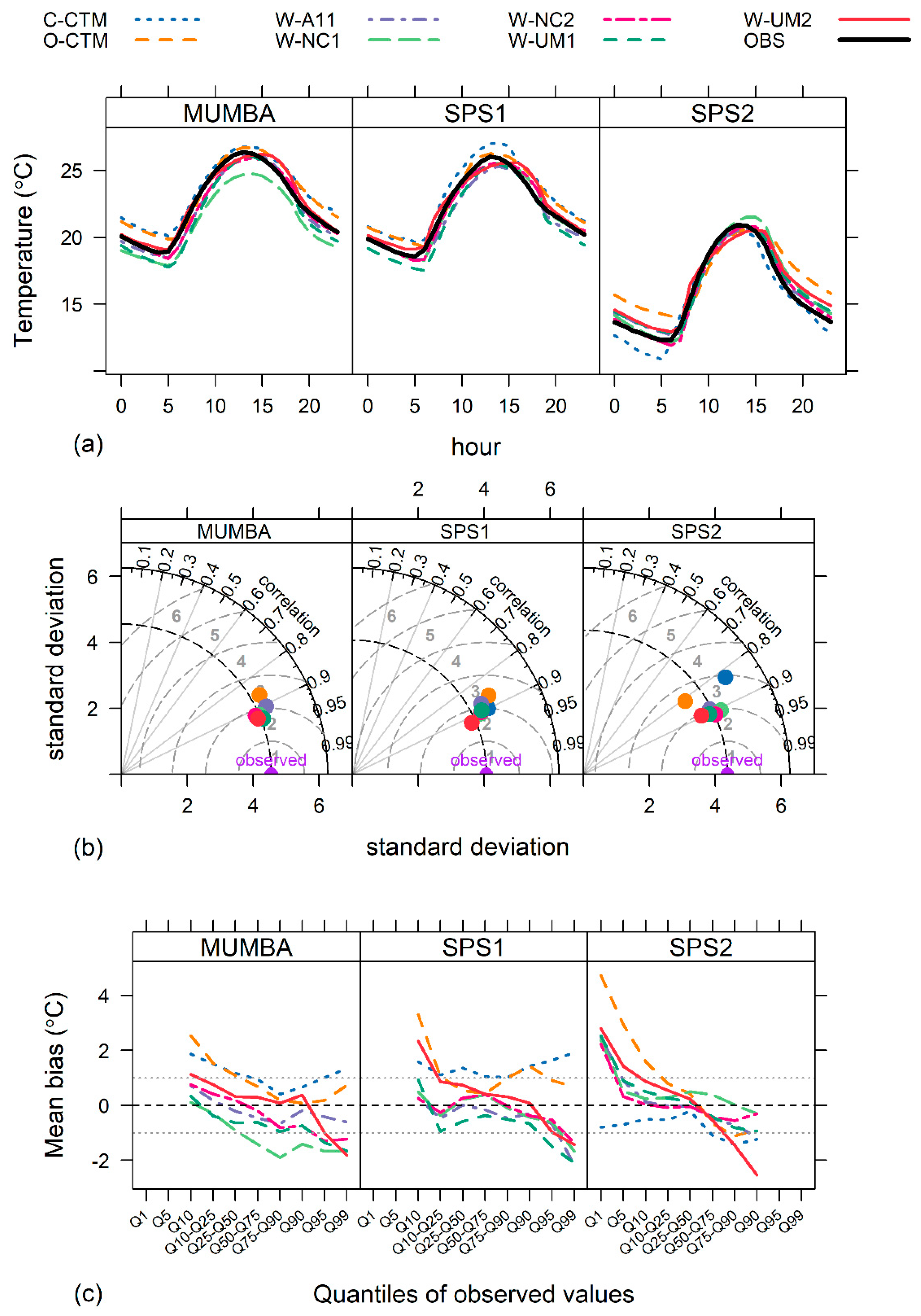
3.1. Temperature
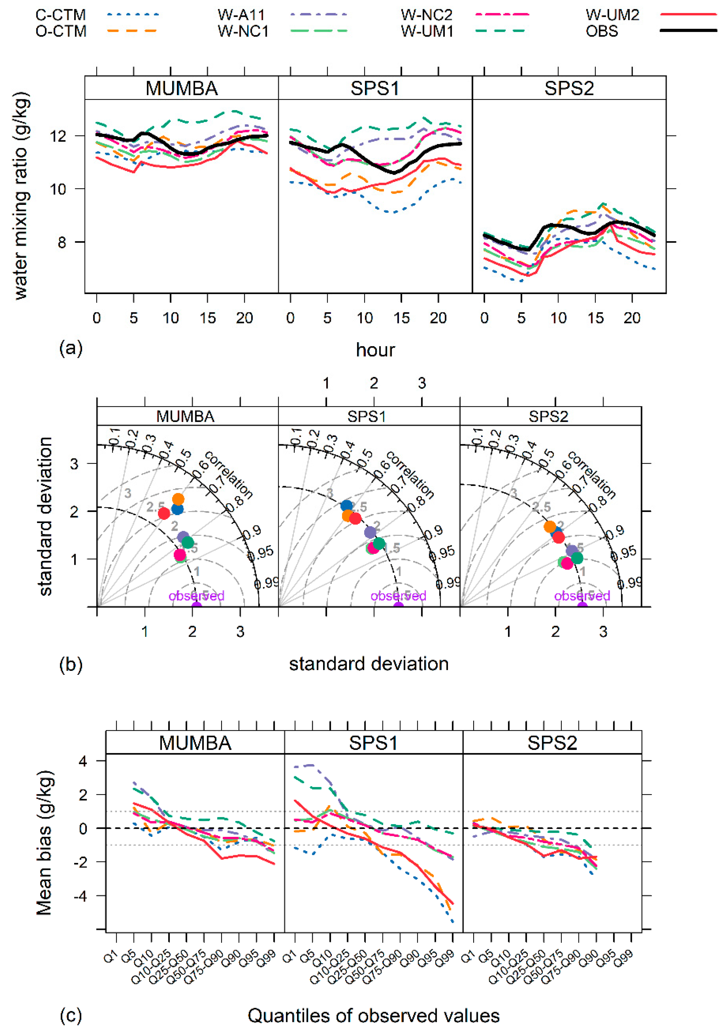
3.2. Mixing Ratio of Water
3.3. Wind
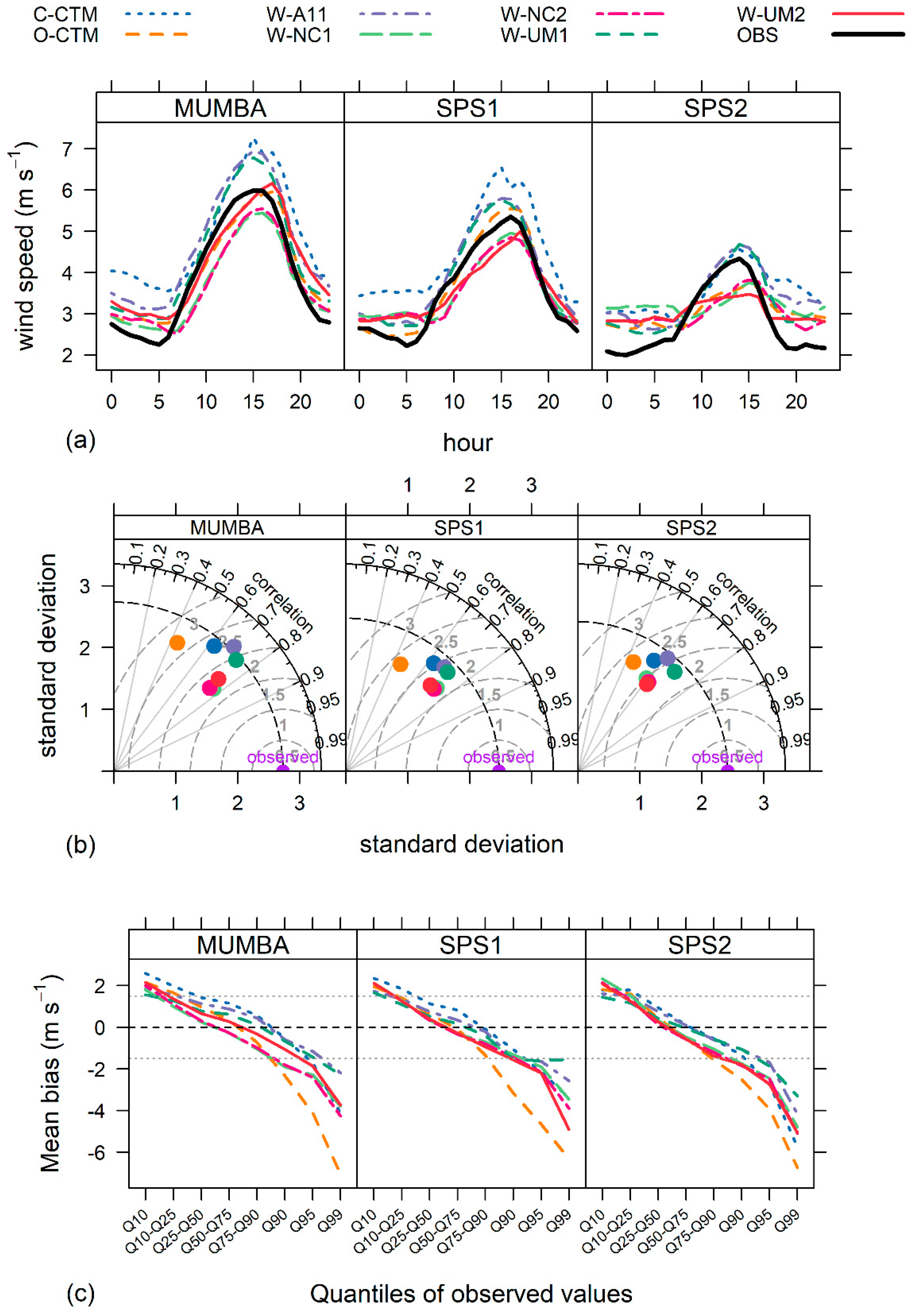
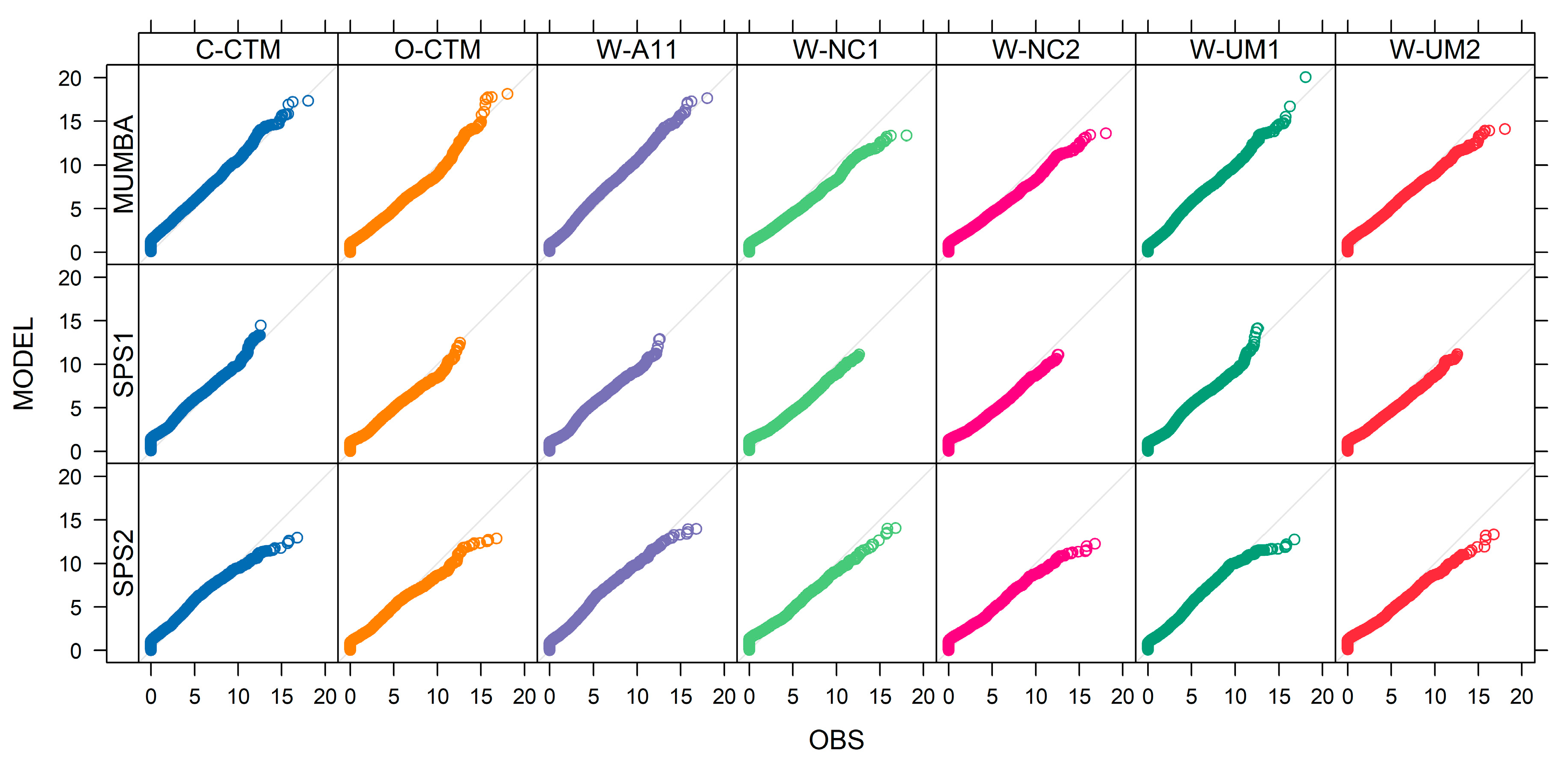
3.3.1. Wind Speed
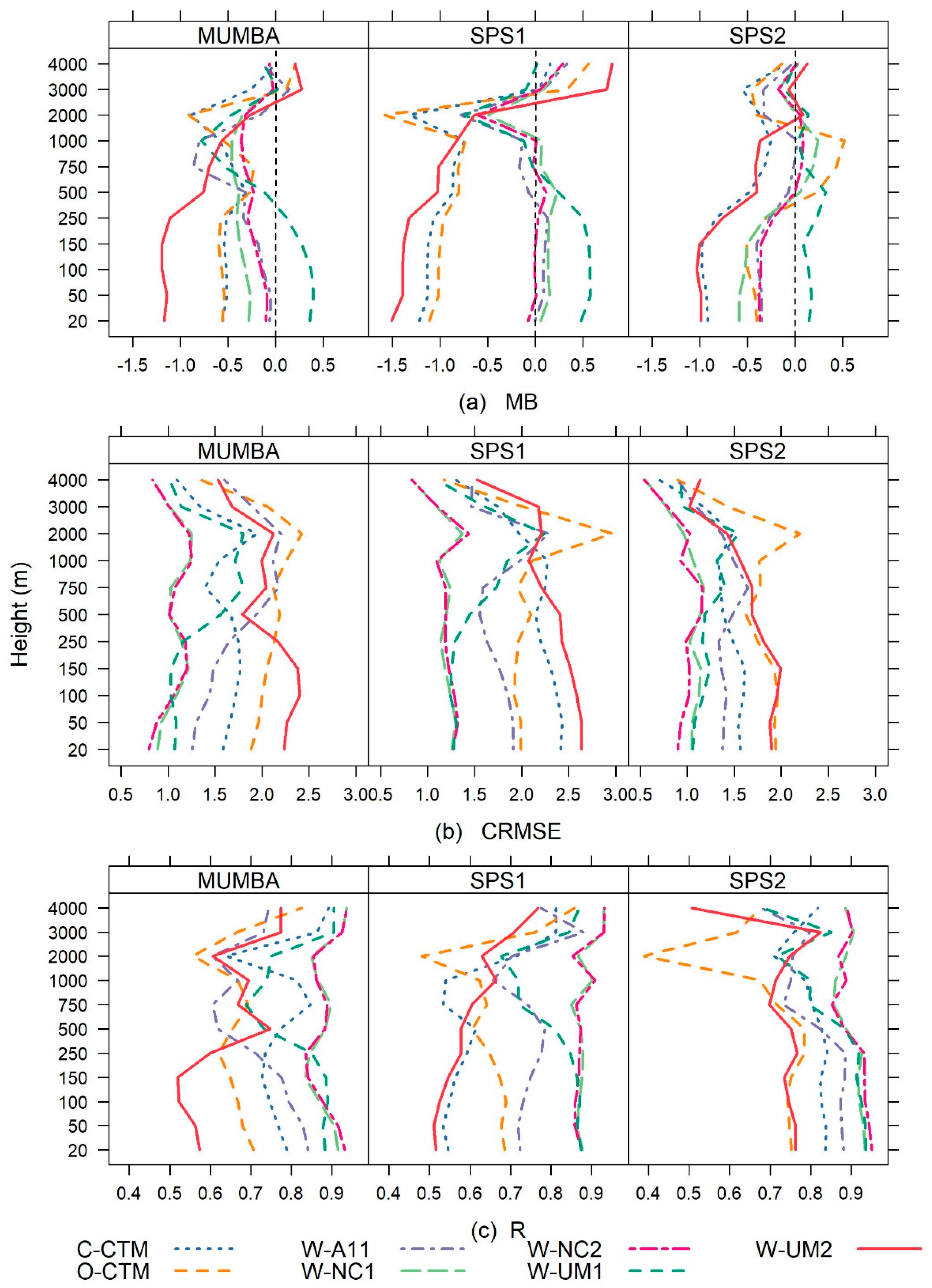
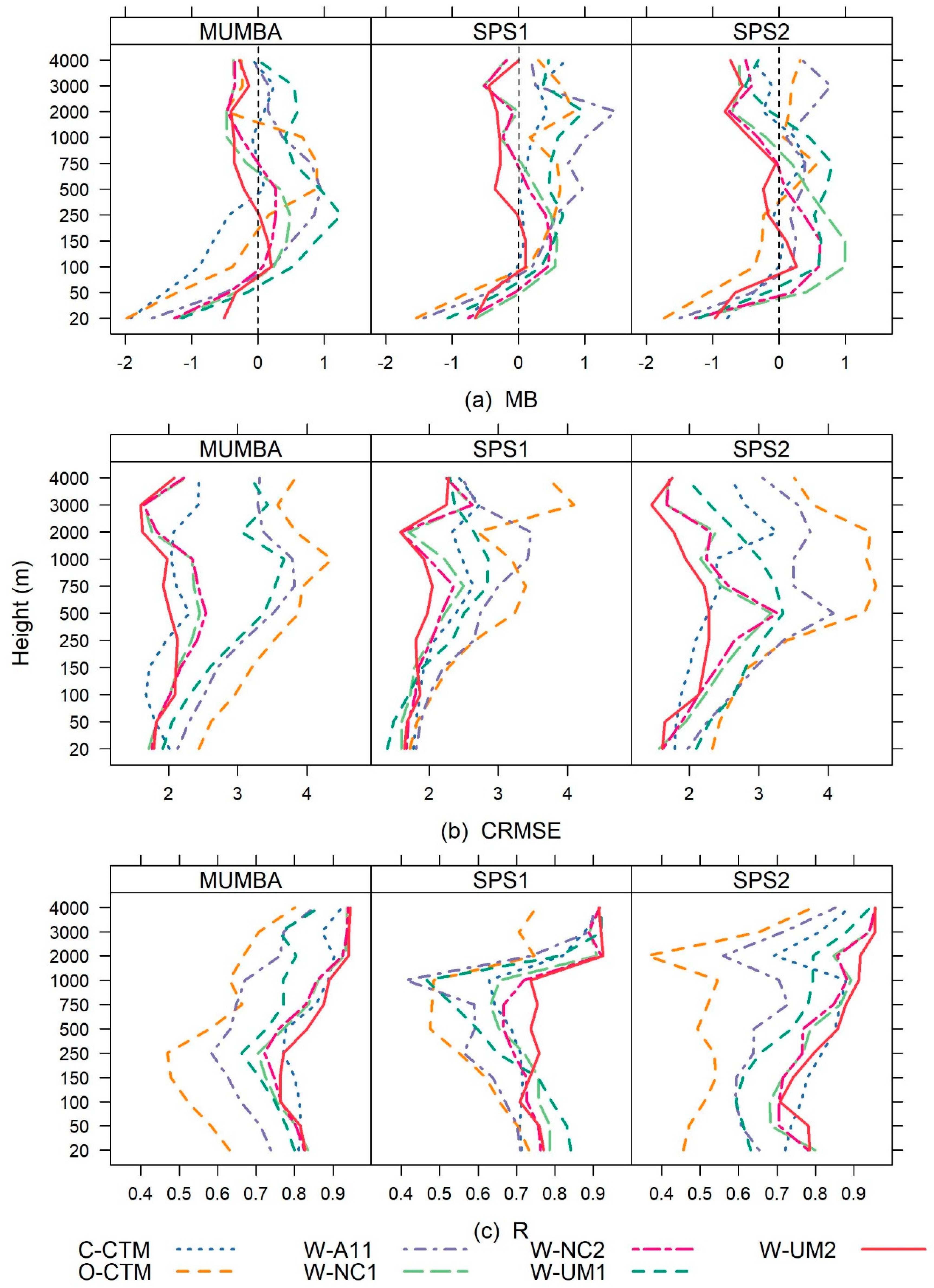
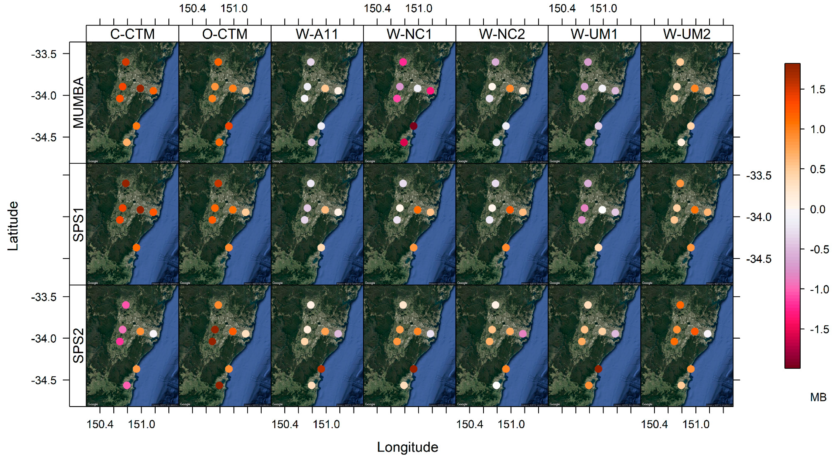
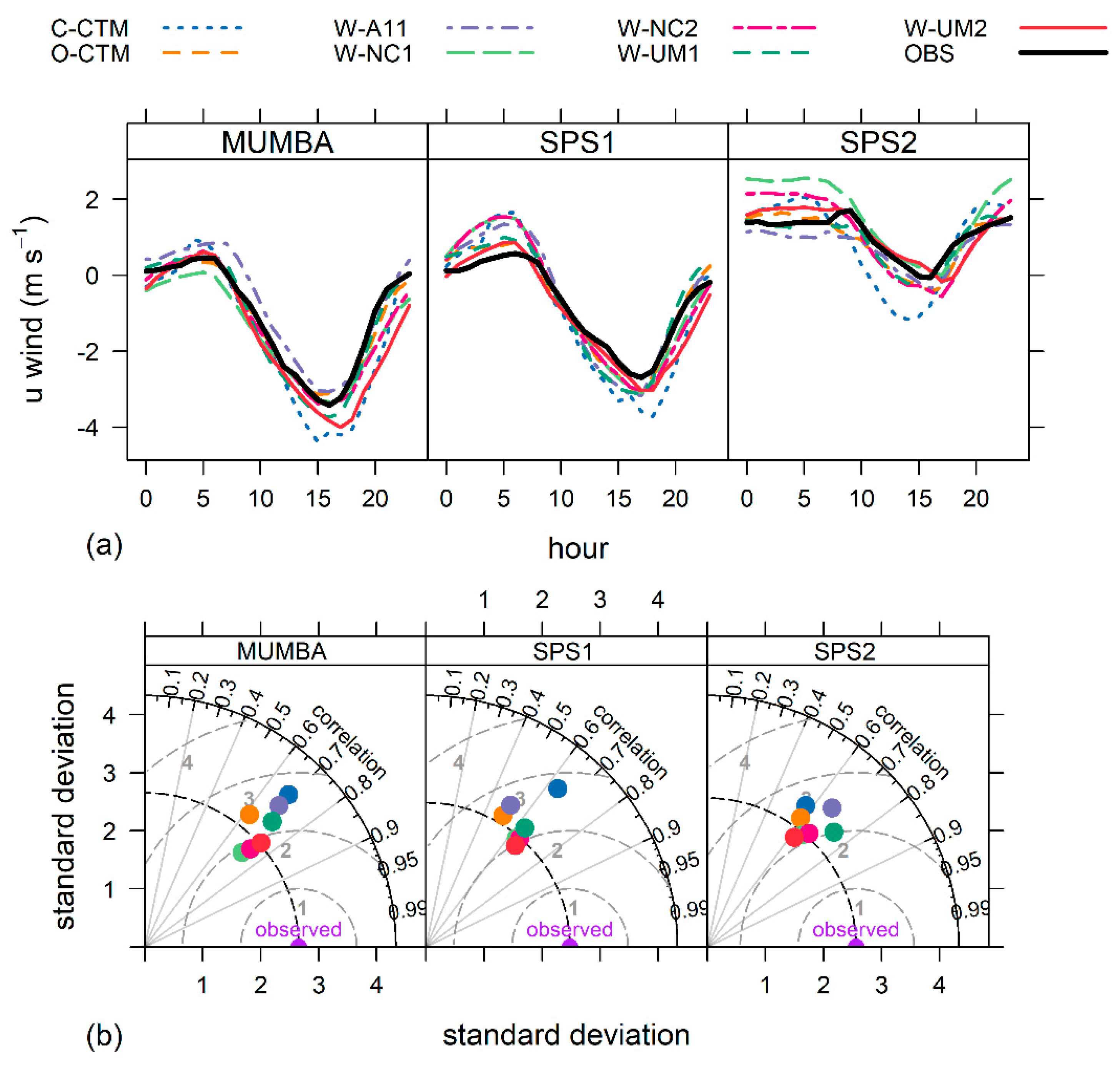
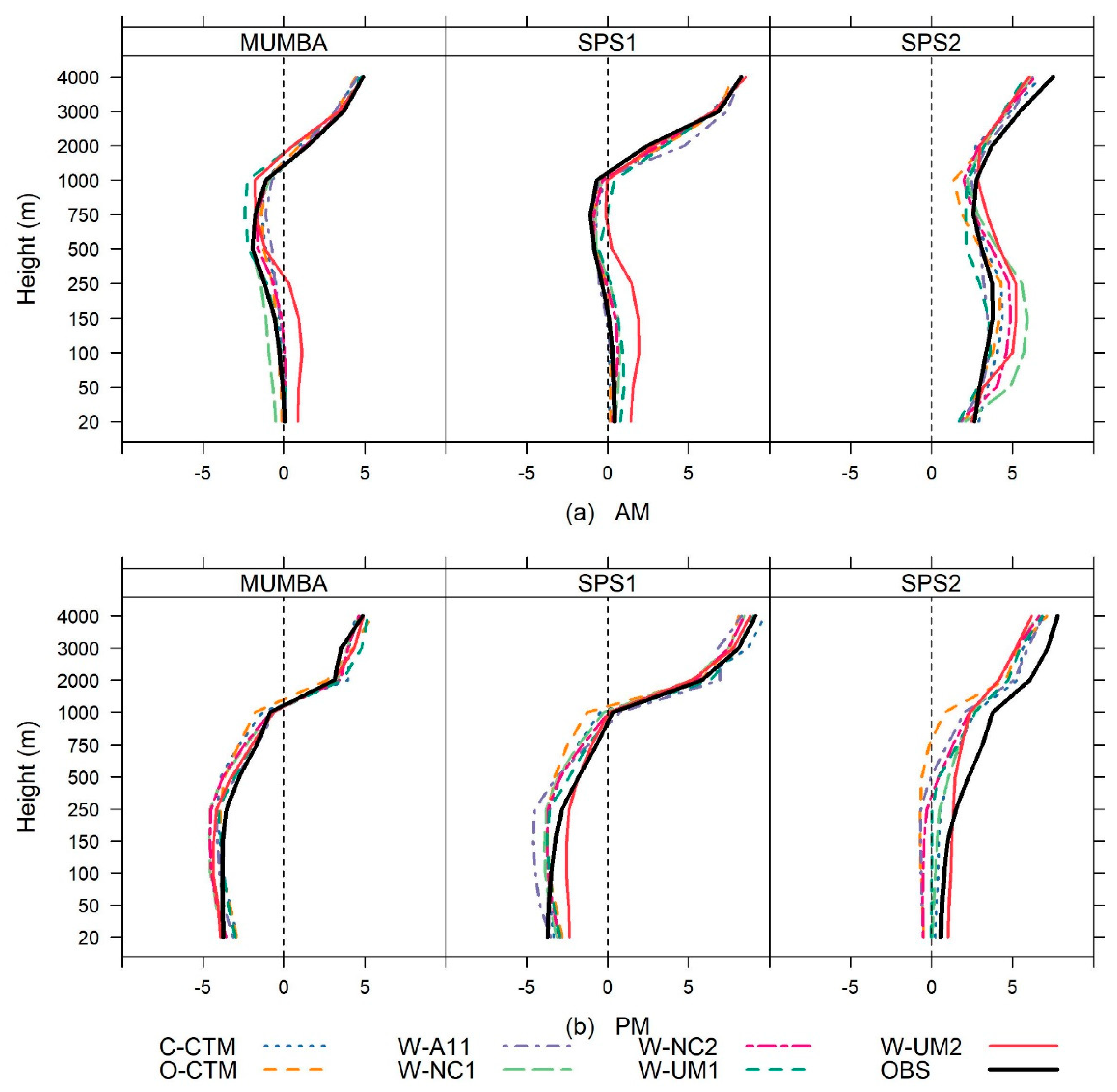
3.3.2. Winds Components
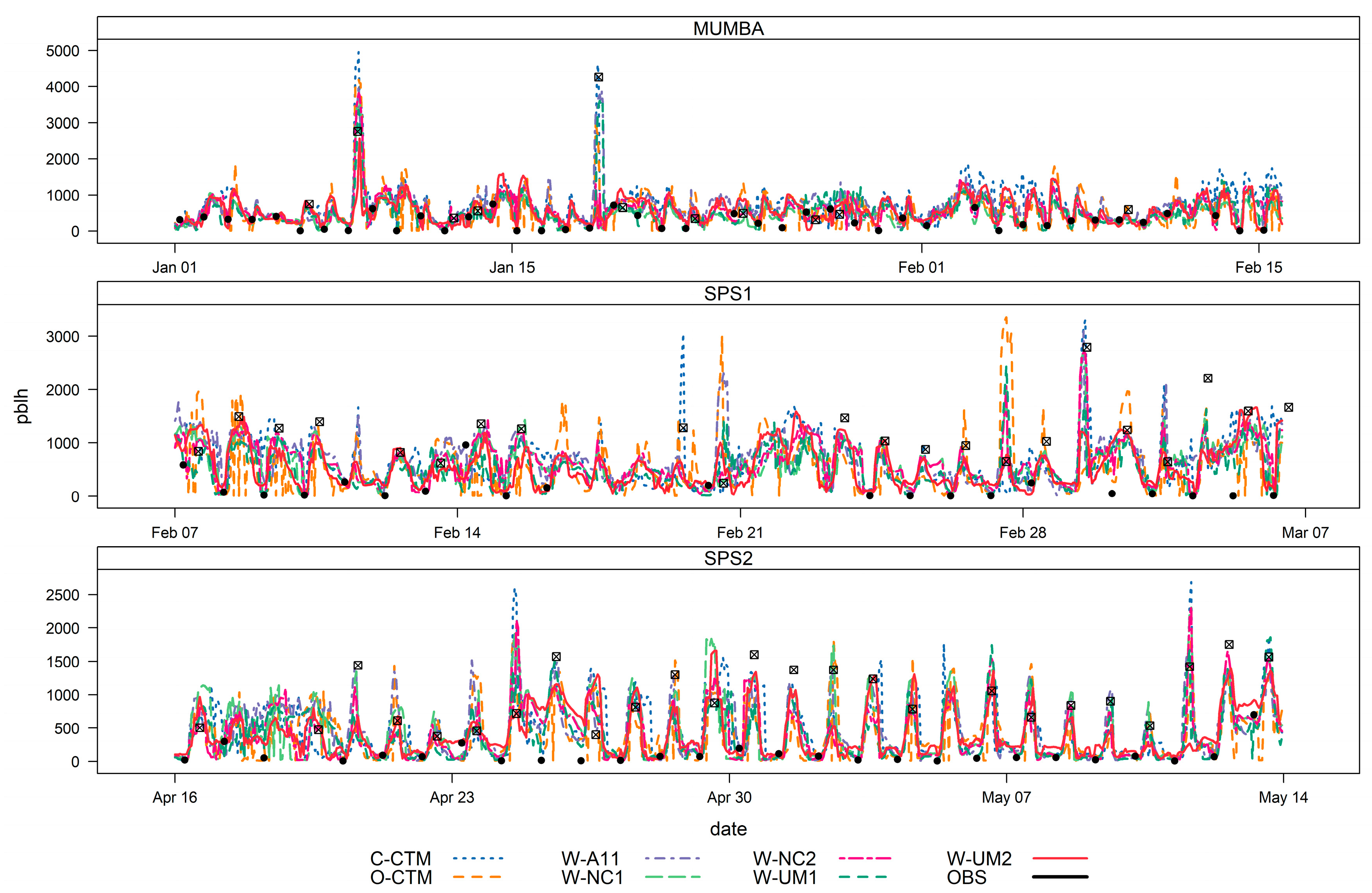
3.4. Planetary Boundary Layer Height
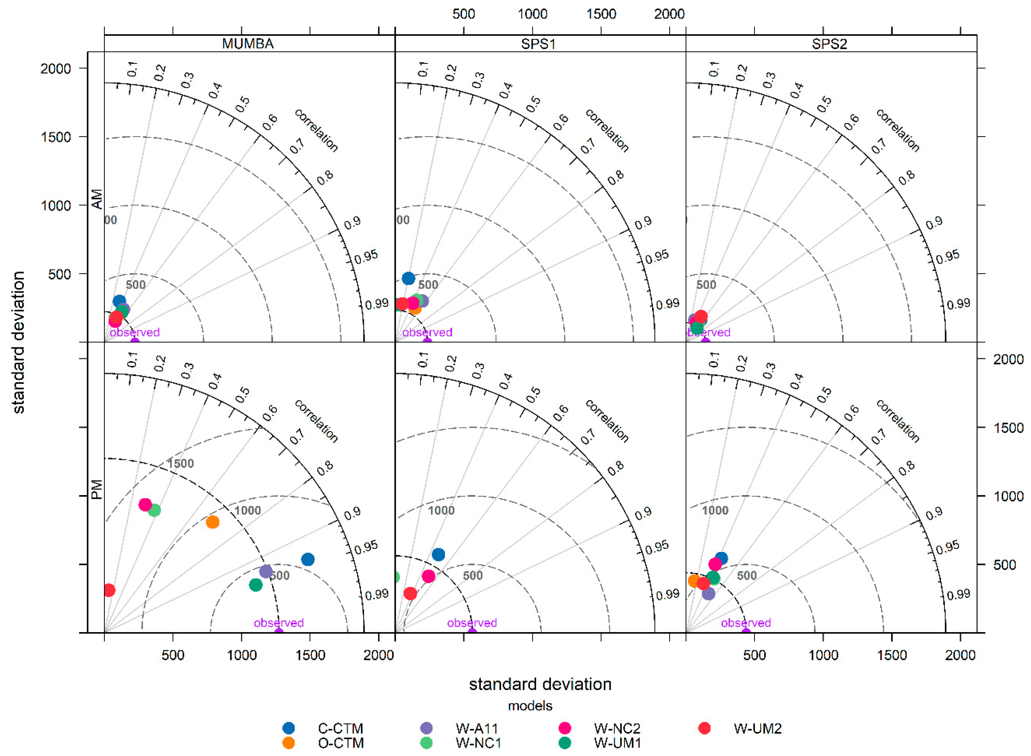
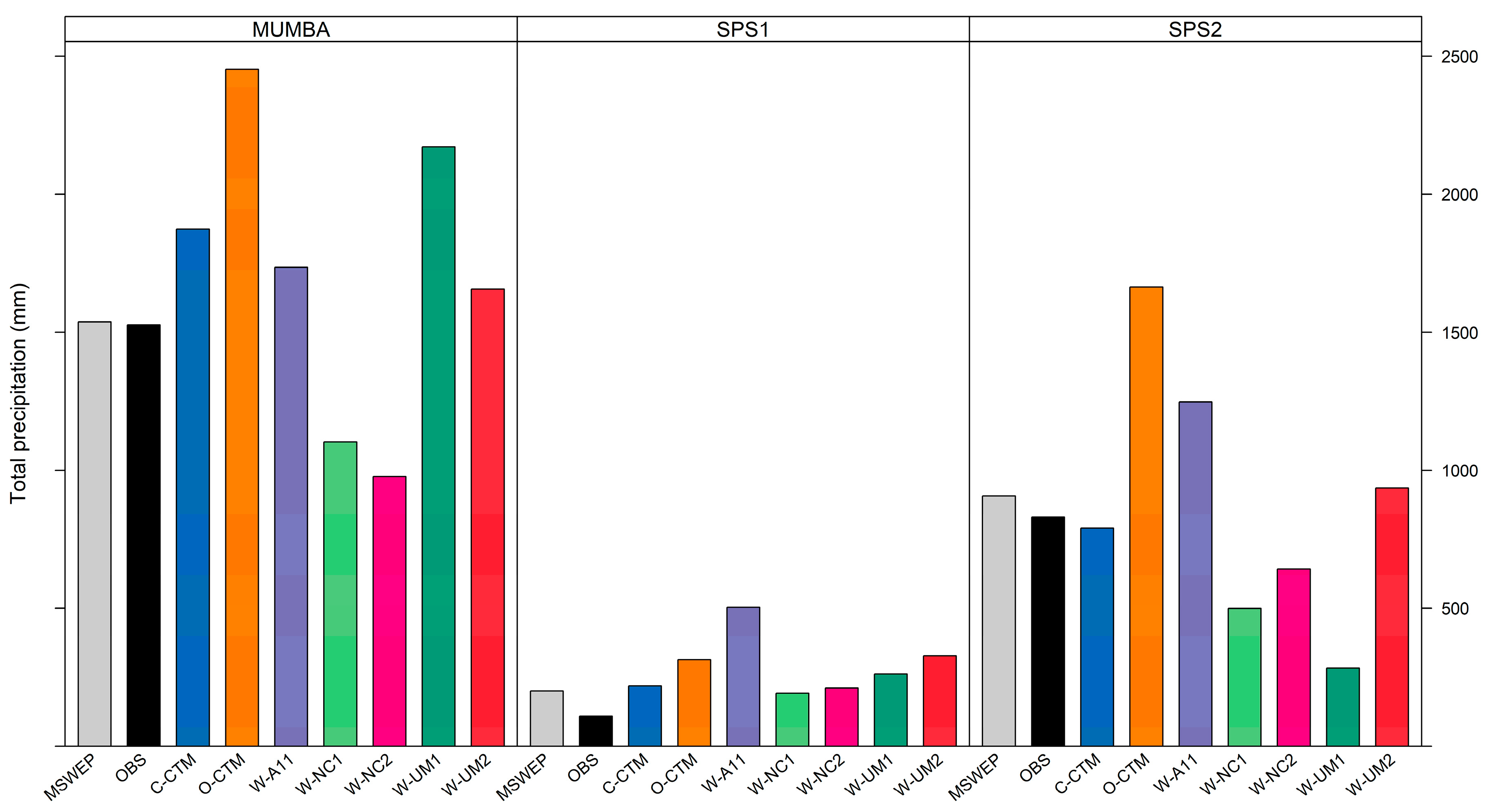
3.5. Precipitation
4. Conclusions
- The near surface air temperatures on average are accurately predicted by the WRF models, with biases within ±2 °C and CRMSE <2 °C. There are larger biases (within ±3 °C) and CRMSE up to 3 °C seen in the daytime near surface temperatures in the CCAM simulations. There is a potential for these biases to impact on photochemistry as they do occur when temperatures peak. The largest temperature biases (up to 5 °C) are seen in the nocturnal temperature, which may be associated with the model’s inability to simulate stable conditions overnight and could impact on dispersion in subsequent air quality modelling.
- Most models show a consistently drier atmosphere than observed, that is largest overnight (<−6 g/kg), while several the WRF simulations overestimate daytime moisture (up to 4 g/kg).
- The biases in temperature and atmospheric moisture in both CCAM simulations may be the result of biases from land surface fluxes. Further investigations into the ideal spin-up length and choice of LSM may reduce these biases.
- The wind speeds were consistently over predicted overnight, which is a common issue with meteorological models. The impact of these biases would lead to underestimation of pollutants overnight due to overestimated dispersion/advection. All simulations tend to underestimate the higher wind speeds.
- The models appear to have the ability to simulate the local-scale meteorological features, like the sea breeze, which is critical to ozone formation over the Sydney Basin. Further analysis into the capability of the models to emulate the progression of the sea breeze front is recommended.
- The PBLH evaluation highlighted some timing differences in the formation of the PBL, which would likely impact simulated morning dispersion. However, the discrete nature of the observations makes it challenging to fully identify the cause of the biases. Some of the models did better than others at capturing PBLH peaks during MUMBA, with the WRF MYJ PBL scheme showing better performance predicting deep convection during hot days compared to YSU. Neither PBL scheme showed better performance for deep convection not associated with extreme temperatures.
- Simulated total accumulated precipitation was overestimated by most models across all campaigns. The W-NC simulations, which used the MSKF cumulus scheme, tended to underestimate total precipitation from a reduction in convective rainfall over the region. Further investigations into the optimal cumulus parameterisation for the Australian region may shed some light on the biases observed.
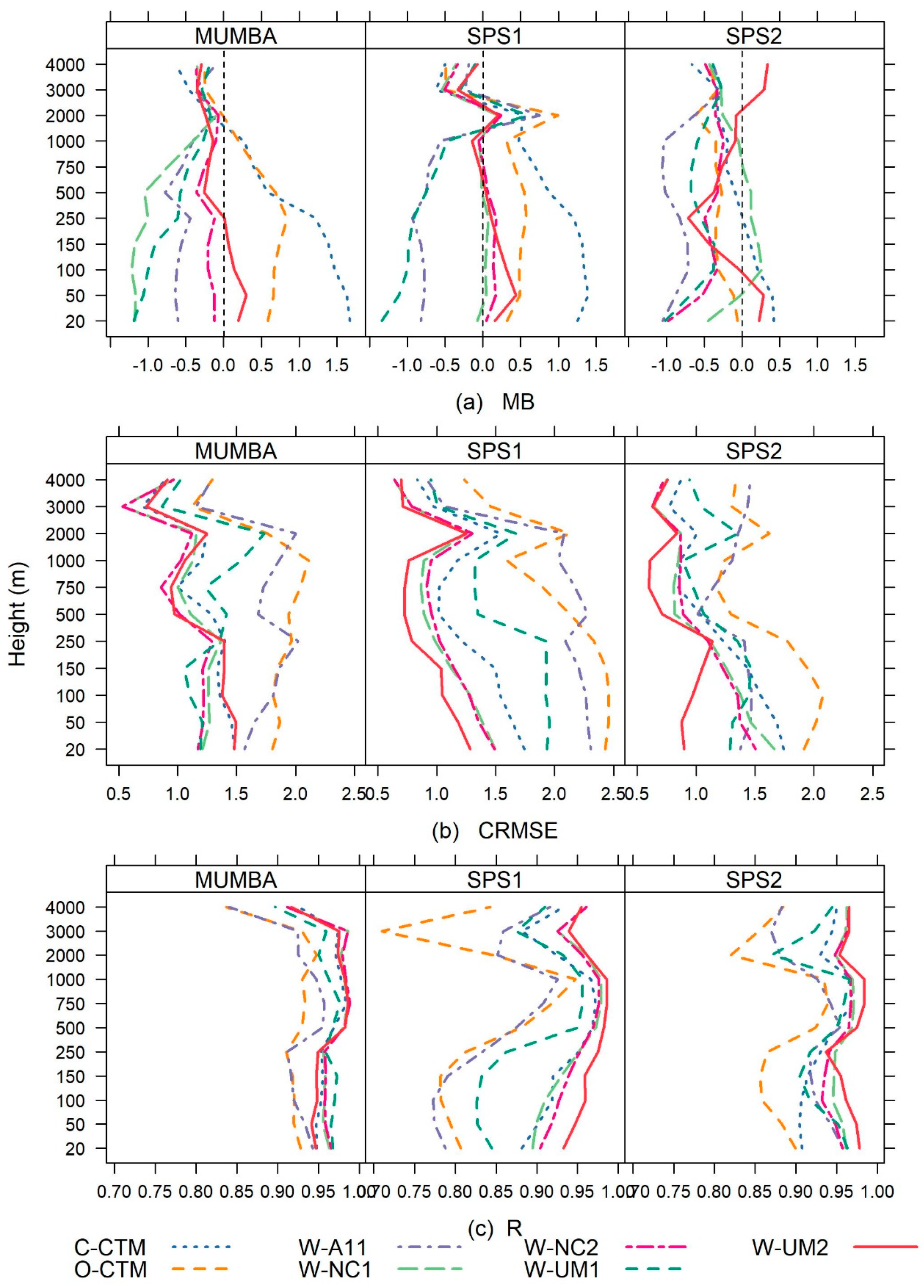
- The simulations with stronger nudging (both W-NC simulations) had improved skill through the vertical profiles compared to the weaker scale selective spectral nudging in W-A11 and CCAM simulations.
Supplementary Materials
Author Contributions
Funding
Acknowledgments
Conflicts of Interest
References
- Lelieveld, J.; Evans, J.S.; Fnais, M.; Giannadaki, D.; Pozzer, A. The contribution of outdoor air pollution sources to premature mortality on a global scale. Nature 2015, 525, 367–371. [Google Scholar] [CrossRef] [PubMed]
- Shah, A.S.V.; Langrish, J.P.; Nair, H.; McAllister, D.A.; Hunter, A.L.; Donaldson, K.; Newby, D.E.; Mills, N.L. Global association of air pollution and heart failure: A systematic review and meta-analysis. Lancet 2013, 382, 1039–1048. [Google Scholar] [CrossRef]
- Keywood, M.D.; Emmerson, K.M.; Hibberd, M.F. Australia State of the Environment 2016: Atmosphere. In Independent Report to the Australian Government Minister for the Environment and Energy; Australian Government Department of the Environment and Energy: Canberra, Australia, 2016. [Google Scholar] [CrossRef]
- Broome, R.A.; Fann, N.; Cristina, T.J.; Fulcher, C.; Duc, H.; Morgan, G.G. The health benefits of reducing air pollution in Sydney, Australia. Environ. Res. 2015, 143, 19–25. [Google Scholar] [CrossRef] [PubMed]
- DP&E. New South Wales State and Local Government Area Population and Household Projections; DP&E: Sydney, NSW, Australia, 2016.
- Cope, M.E.; Keywood, M.D.; Emmerson, K.M.; Galbally, I.E.; Boast, K.; Chambers, S.; Cheng, M.; Crumeyrolle, S.; Dunne, E.; Fedele, R.; et al. Sydney Particle Study—Stage II; The Centre for Australian Weather and Climate Research: Melbourne, Australia, 2014; ISBN 978-1-4863-0359-5.
- Seaman, N.L. Meteorological modeling for air-quality assessments. Atmos. Environ. 2000, 34, 2231–2259. [Google Scholar] [CrossRef]
- Chambers, S.; Guerette, E.-A.; Monk, K.; Griffiths, A.D.; Zhang, Y.; Nguyen Duc, H.; Cope, M.E.; Emmerson, K.M.; Chang, L.T.-C.; Silver, J.D.; et al. Skill-testing chemical transport models across contrasting atmospheric mixing states using Radon-222. Atmosphere 2019, 10, 25. [Google Scholar] [CrossRef]
- Zhang, F.; Bei, N.; Nielsen-Gammon, J.W.; Li, G.; Zhang, R.; Stuart, A.; Aksoy, A. Impacts of meteorological uncertainties on ozone pollution predictability estimated through meteorological and photochemical ensemble forecasts. J. Geophys. Res. 2007, 112. [Google Scholar] [CrossRef]
- Rao, S.T.; Galmarini, S.; Puckett, K. Air Quality Model Evaluation International Initiative (AQMEII): Advancing the State of the Science in Regional Photochemical Modeling and Its Applications. Bull. Am. Meteorol. Soc. 2011, 92, 23–30. [Google Scholar] [CrossRef]
- Vautard, R.; Moran, M.D.; Solazzo, E.; Gilliam, R.C.; Matthias, V.; Bianconi, R.; Chemel, C.; Ferreira, J.; Geyer, B.; Hansen, A.B.; et al. Evaluation of the meteorological forcing used for the Air Quality Model Evaluation International Initiative (AQMEII) air quality simulations. Atmos. Environ. 2012, 53, 15–37. [Google Scholar] [CrossRef]
- Solazzo, E.; Bianconi, R.; Pirovano, G.; Matthias, V.; Vautard, R.; Moran, M.D.; Wyat Appel, K.; Bessagnet, B.; Brandt, J.; Christensen, J.H.; et al. Operational model evaluation for particulate matter in Europe and North America in the context of AQMEII. Atmos. Environ. 2012, 53, 75–92. [Google Scholar] [CrossRef]
- Solazzo, E.; Bianconi, R.; Vautard, R.; Appel, K.W.; Moran, M.D.; Hogrefe, C.; Bessagnet, B.; Brandt, J.; Christensen, J.H.; Chemel, C.; et al. Model evaluation and ensemble modelling of surface-level ozone in Europe and North America in the context of AQMEII. Atmos. Environ. 2012, 53, 60–74. [Google Scholar] [CrossRef]
- Brunner, D.; Savage, N.; Jorba, O.; Eder, B.; Giordano, L.; Badia, A.; Balzarini, A.; Baró, R.; Bianconi, R.; Chemel, C.; et al. Comparative analysis of meteorological performance of coupled chemistry-meteorology models in the context of AQMEII phase 2. Atmos. Environ. 2015, 115, 470–498. [Google Scholar] [CrossRef]
- Im, U.; Bianconi, R.; Solazzo, E.; Kioutsioukis, I.; Badia, A.; Balzarini, A.; Baró, R.; Bellasio, R.; Brunner, D.; Chemel, C.; et al. Evaluation of operational online-coupled regional air quality models over Europe and North America in the context of AQMEII phase 2. Part II: Particulate matter. Atmos. Environ. 2015, 115, 421–441. [Google Scholar] [CrossRef]
- Im, U.; Bianconi, R.; Solazzo, E.; Kioutsioukis, I.; Badia, A.; Balzarini, A.; Baró, R.; Bellasio, R.; Brunner, D.; Chemel, C.; et al. Evaluation of operational on-line-coupled regional air quality models over Europe and North America in the context of AQMEII phase 2. Part I: Ozone. Atmos. Environ. 2015, 115, 404–420. [Google Scholar] [CrossRef]
- Angevine, W.M.; Eddington, L.; Durkee, K.; Fairall, C.; Bianco, L.; Brioude, J. Meteorological Model Evaluation for CalNex 2010. Mon. Weather Rev. 2012, 140, 3885–3906. [Google Scholar] [CrossRef]
- Carslaw, D.; Agnew, P.; Beevers, S.; Chemel, C.; Cooke, S.; Davis, L.; Derwent, D.; Francis, X.; Fraser, A.; Kitwiroon, N.; et al. Defra Phase 2 Regional Model Evaluation; DEFRA: London, UK, 2013.
- NSW-EPA. 2008 Calendar Year Air Emissions Inventory for the Greater Metropolitan Region in New South Wales; NSW-Environment Protection Authority: Sydney, Australia, 2012.
- NSW-OEH. Towards Cleaner Air. NSW Air Quality Statement 2016; NSW-OEH: Sydney, Australia, 2016.
- Utembe, S.; Rayner, P.; Silver, J.; Guerette, E.-A.; Fisher, J.; Emmerson, K.; Cope, M.E.; Paton-Walsh, C.; Griffiths, A.; Duc, H.; et al. Hot summers: Effect of elevated temperature on air quality in Sydney, Australia. Atmosphere 2018, 9, 466. [Google Scholar] [CrossRef]
- Price, O.F.; Williamson, G.J.; Henderson, S.B.; Johnston, F.; Bowman, D.M. The relationship between particulate pollution levels in Australian cities, meteorology, and landscape fire activity detected from MODIS hotspots. PLoS ONE 2012, 7, e47327. [Google Scholar] [CrossRef] [PubMed]
- Di Virgilio, G.; Hart, M.A.; Jiang, N.B. Meteorological controls on atmospheric particulate pollution during hazard reduction burns. Atmos. Chem. Phys. 2018, 18, 6585–6599. [Google Scholar] [CrossRef]
- Williamson, G.J.; Bowman, D.M.J.S.; Price, O.F.; Henderson, S.B.; Johnston, F.H. A transdisciplinary approach to understanding the health effects of wildfire and prescribed fire smoke regimes. Environ. Res. Lett. 2016, 11, 125009. [Google Scholar] [CrossRef]
- Williamson, G.; Price, O.; Henderson, S.; Bowman, D. Satellite-based comparison of fire intensity and smoke plumes from prescribed and wildfires in south-eastern Australia. Int. J. Wildland Fire J. 2013, 22, 121–129. [Google Scholar] [CrossRef]
- Hyde, R.; Young, M.A.; Hurley, P.; Manins, P.C. Metropolitan Air Quality Study Meteorology—Air Movements; NSW Environmental Protection Authority: Sydney, Australia, 1996.
- Hart, M.; De Dear, R.; Hyde, R. A synoptic climatology of tropospheric ozone episodes in Sydney, Australia. Int. J. Climatol. 2006, 26, 1635–1649. [Google Scholar] [CrossRef]
- Jiang, N.; Betts, A.; Riley, M. Summarising climate and air quality (ozone) data on self-organising maps: A Sydney case study. Environ. Monit. Assess. 2016, 188, 103. [Google Scholar] [CrossRef] [PubMed]
- Paton-Walsh, C.; Guérette, É.-A.; Emmerson, K.; Cope, M.; Kubistin, D.; Humphries, R.; Wilson, S.; Buchholz, R.; Jones, N.; Griffith, D.; et al. Urban Air Quality in a Coastal City: Wollongong during the MUMBA Campaign. Atmosphere 2018, 9, 500. [Google Scholar] [CrossRef]
- Crippa, P.; Sullivan, R.C.; Thota, A.; Pryor, S.C. The impact of resolution on meteorological, chemical and aerosol properties in regional simulations with WRF-Chem. Atmos. Chem. Phys. 2017, 17, 1511–1528. [Google Scholar] [CrossRef]
- Skamarock, W.C.; Klemp, J.B.; Dudhia, J.; Gill, D.O.; Barker, D.M.; Duda, M.G.; Huang, X.-Y.; Wang, W.; Powers, J.G. A Description of the Advanced Research WRF Version 3. NCAR Tech. Note 2008. [Google Scholar] [CrossRef]
- McGregor, J.; Dix, M.R. An Updated Description of the Conformal-Cubic Atmospheric Model. In High Resolution Simulation of the Atmosphere and Ocean; Hamilton, K., Ohfuchi, W., Eds.; Springer: Berlin, Germany, 2008. [Google Scholar]
- Guerette, E.-A.; Monk, K.; Utembe, S.; Silver, J.D.; Emmerson, K.; Griffiths, A.; Duc, H.; Chang, L.T.-C.; Trieu, T.; Jiang, N.; et al. Evaluation of regional air quality models over Sydney, Australia: Part 2 Model performance for surface ozone and PM2.5. Atmosphere 2019. submitted. [Google Scholar]
- Dee, D.P.; Uppala, S.M.; Simmons, A.J.; Berrisford, P.; Poli, P.; Kobayashi, S.; Andrae, U.; Balmaseda, M.A.; Balsamo, G.; Bauer, P.; et al. The ERA-Interim reanalysis: Configuration and performance of the data assimilation system. Q. J. 2011, 137, 553–597. [Google Scholar] [CrossRef]
- NCEP FNL Operational Model Global Tropospheric Analyses, continuing from July 1999. In Research Data Archive at the National Center for Atmospheric Research; Computational and Information Systems Laboratory: Boulder, CO, USA, 2000. [CrossRef]
- Janjić, Z.I. The Step-Mountain Eta Coordinate Model: Further Developments of the Convection, Viscous Sublayer, and Turbulence Closure Schemes. Mon. Weather Rev. 1994, 122, 927–945. [Google Scholar] [CrossRef]
- Hong, S.-Y.; Noh, Y.; Dudhia, J. A New Vertical Diffusion Package with an Explicit Treatment of Entrainment Processes. Mon. Weather Rev. 2006, 134, 2318. [Google Scholar] [CrossRef]
- Lin, Y.-L.; Farely, R.D.; Orville, H.D. Bulk parameterization of the snow field in a cloud model. J. Appl. Meteorol. Climatol. 1983, 22, 1065–1092. [Google Scholar] [CrossRef]
- Hong, S.-Y.; Lim, J.-O. The WRF Single-Moment 6-Class Microphysics Scheme (WSM6). J. Korean Meteor. Soc. 2006, 42, 129–151. [Google Scholar]
- Morrison, H.; Thompson, G.; Tatarskii, V. Impact of Cloud Microphysics on the Development of Trailing Stratiform Precipitation in a Simulated Squall Line: Comparison of One- and Two-Moment Schemes. Mon. Weather Rev. 2009, 137, 991–1007. [Google Scholar] [CrossRef]
- Grell, G.A.; Dévényi, D. A generalized approach to parameterizing convection combining ensemble and data assimilation techniques. Geophys. Res. Lett. 2002, 29. [Google Scholar] [CrossRef]
- Zheng, Y.; Alapaty, K.; Herwehe, J.A.; Del Genio, A.D.; Niyogi, D. Improving High-Resolution Weather Forecasts Using the Weather Research and Forecasting (WRF) Model with an Updated Kain–Fritsch Scheme. Mon. Weather Rev. 2016, 144, 833–860. [Google Scholar] [CrossRef]
- Iacono, M.J.; Delamere, J.S.; Mlawer, E.J.; Shephard, M.W.; Clough, S.A.; Collins, W.D. Radiative forcing by long-lived greenhouse gases: Calculations with the AER radiative transfer models. J. Geophys. Res. Atmos. 2008, 113. [Google Scholar] [CrossRef]
- Chou, M.-D.; Suarez, M.J. A Solar Radiation Parameterization (CLIRAD-SW) for Atmospheric Studies; NASA/TM-1999-104606; NASA Goddard Space Flight Center: Greenbelt, MD, USA, 1999.
- Chou, M.-D.; Suarez, M.J.; Liang, X.-Z.; Yan, M.M.-H. A Thermal Infrared Radiation Parameterisation for Atmospheric Studies; NASA/TM-2001-104606; NASA Goddard Space Flight Center: Greenbelt, MD, USA, 2001.
- Chen, F.; Dudhia, J. Coupling an Advanced Land Surface-Hydrology Model with the Penn State-NCAR MM5 Modeling System. Part 1: Model Implementation and Sensitivity. Mon. Weather Rev. 2001, 129. [Google Scholar] [CrossRef]
- He, J.; He, R.; Zhang, Y. Impacts of Air-sea Interactions on Regional Air Quality Predictions Using a Coupled Atmosphere-ocean Model in South-eastern U.S. Aerosol Air Q. Res. 2018, 18, 1044–1067. [Google Scholar] [CrossRef]
- Wang, K.; Zhang, Y.; Yahya, K.; Wu, S.-Y.; Grell, G. Implementation and initial application of new chemistry-aerosol options in WRF/Chem for simulating secondary organic aerosols and aerosol indirect effects for regional air quality. Atmos. Environ. 2015, 115, 716–732. [Google Scholar] [CrossRef]
- Zhang, Y.; Jena, C.; Wang, K.; Paton-Walsh, C.; Guérette, É.-A.; Utembe, S.; Silver, D.J.; Keywood, M. Multiscale Applications of Two Online-Coupled Meteorology-Chemistry Models during Recent Field Campaigns in Australia, Part I: Model Description and WRF/Chem-ROMS Evaluation Using Surface and Satellite Data and Sensitivity to Spatial Grid Resolutions. Atmosphere 2019, 10, 189. [Google Scholar] [CrossRef]
- Zhang, Y.; Wang, K.; Jena, C.; Paton-Walsh, C.; Guérette, É.-A.; Utembe, S.; Silver, D.J.; Keywood, M. Multiscale Applications of Two Online-Coupled Meteorology-Chemistry Models during Recent Field Campaigns in Australia, Part II: Comparison of WRF/Chem and WRF/Chem-ROMS and Impacts of Air-Sea Interactions and Boundary Conditions. Atmosphere 2019, 10, 210. [Google Scholar] [CrossRef]
- McGregor, J. C-CAM Geometric Aspects and Dynamical Formulation; CSIRO Marine and Atmospheric Research: Aspendale, Australia, 2005; p. 70.
- Schmidt, F. Variable fine mesh in the spectral global models. Beitraege Physik Atmos. 1977, 50, 211–217. [Google Scholar]
- Corney, S.; Grose, M.; Bennett, J.C.; White, C.; Katzfey, J.; McGregor, J.; Holz, G.; Bindoff, N.L. Performance of downscaled regional climate simulations using a variable-resolution regional climate model: Tasmania as a test case. J. Geophys. Res. Atmos. 2013, 118, 11936–11950. [Google Scholar] [CrossRef]
- Nguyen, K.C.; Katzfey, J.J.; McGregor, J.L. Downscaling over Vietnam using the stretched-grid CCAM: Verification of the mean and interannual variability of rainfall. Clim. Dyn. 2013, 43, 861–879. [Google Scholar] [CrossRef][Green Version]
- Emmerson, K.M.; Galbally, I.E.; Guenther, A.B.; Paton-Walsh, C.; Guerette, E.-A.; Cope, M.E.; Keywood, M.D.; Lawson, S.J.; Molloy, S.B.; Dunne, E.; et al. Current estimates of biogenic emissions from eucalypts uncertain for southeast Australia. Atmos. Chem. Phys. 2016, 16, 6997–7011. [Google Scholar] [CrossRef]
- Emmerson, K.M.; Cope, M.E.; Galbally, I.E.; Lee, S.; Nelson, P.F. Isoprene and monoterpene emissions in south-east Australia: Comparison of a multi-layer canopy model with MEGAN and with atmospheric observations. Atmos. Chem. Phys. 2018, 18, 7539–7556. [Google Scholar] [CrossRef]
- Kowalczyk, E.A.; Garratt, J.R.; Krummel, P.B. Implementation of a Soil-Canopy Scheme into CSIRO GCM—Regional Aspects of the Model Response. CSIRO Atmos. Res. Tech. Pap. 1994, 32. [Google Scholar] [CrossRef]
- Thatcher, M. Processing of Global Land Surface Datasets for Dynamical Downscaling with CCAM and TAPM; CSIRO Marine and Atmospheric Research: Aspendale, Australia, 2008.
- Schwarzkopf, M.D.; Fels, S.B. The Simplified Exchange Method Revisited: An Accurate, Rapid Method for Computation of Infrared Cooling Rates and Fluxes. J. Geophys. Res. 1991, 96, 9075–9096. [Google Scholar] [CrossRef]
- Rotstayn, L.D. A physically based scheme for the treatment of stratiform clouds and precipitation in large-scale models. I: Description and evaluation of the microphysical processes. Q. J. R. Meteorol. Soc. 1997, 123, 1227–1282. [Google Scholar] [CrossRef]
- McGregor, J.L.; Gordon, H.B.; Watterson, I.G.; Dix, M.R.; Rotstayn, L.D. The CSIRO 9-Level Atmospheric General Circulation Model; CSIRO: Canberra, Australia, 1993; pp. 1–89.
- Holtslag, A.A.M.; Boville, B.A. Local Versus Nonlocal Boundary-Layer Diffusion in a Global Climate Model. J. Clim. 1993, 6, 1825–1842. [Google Scholar] [CrossRef]
- McGregor, J. A New Convection Scheme Using a Simple Closure. BMRC Res. Rep. 2003, 93, 33–36. [Google Scholar]
- Rotstayn, L.D.; Lohmann, U. Tropical Rainfall Trends and the Indirect Aerosol Effect. J. Clim. 2002, 15, 2103–2116. [Google Scholar] [CrossRef]
- Thatcher, M.; Hurley, P. Simulating Australian Urban Climate in a Mesoscale Atmospheric Numerical Model. Boun.-Layer Meteorol. 2012, 142, 149–175. [Google Scholar] [CrossRef]
- Guérette, E.-A.; Paton-Walsh, C.; Kubistin, D.; Humphries, R.; Bhujel, M.; Buchholz, R.R.; Chambers, S.; Cheng, M.; Davy, P.; Dominick, D.; et al. Measurements of Urban, Marine and Biogenic Air (MUMBA): Characterisation of Trace Gases and Aerosol at the Urban, Marine and Biogenic Interface in Summer in Wollongong, Australia; PANGAEA: Wollongong, Australia, 2017. [Google Scholar]
- Paton-Walsh, C.; Guerette, E.-A.; Kubistin, D.C.; Humphries, R.S.; Wilson, S.R.; Dominick, D.; Galbally, I.E.; Buchholz, R.R.; Bhujel, M.; Chambers, S.; et al. The MUMBA campaign: Measurements of urban marine and biogenic air. Earth Syst. Sci. Data 2017, 9, 349–362. [Google Scholar] [CrossRef]
- Dennis, R.; Fox, T.; Fuentes, M.; Gilliland, A.; Hanna, S.; Hogrefe, C.; Irwin, J.; Rao, S.T.; Scheffe, R.; Schere, K.; et al. A Framework for Evaluating Regional-Scale Numerical Photochemical Modeling Systems. Environ. Fluid Mech. 2010, 10, 471–489. [Google Scholar] [CrossRef] [PubMed]
- Emery, C.; Tai, E. Enhanced Meteorological Modeling and Performance Evaluation for Two Texas Ozone Episodes. In Final Report submitted to Texas Near Non-Attainment Areas through the Alamo Area Council of Governments; ENVIRON International Corp.: Novato, CA, USA, 2001. [Google Scholar]
- Kemball-Cook, S.; Jia, Y.; Emery, C.; Morris, R.; Wang, Z.; Tonnesen, G. Alaska MM5 Modeling for the 2002 Annual Period to Support Visibility Modeling. In Prepared for Western Regional Air Partnership (WRAP); Environ International Corporation: Novato, CA, USA, 2005. [Google Scholar]
- McNally, D.E. 12 km MM5 Performance Goals. In Proceedings of the 10th Annual AdHoc Meteorological Modelers Meeting, Boulder, CO, USA, 24–25 June 2010; Environmental Protection Agency: Washington, DC, USA, 2009. [Google Scholar]
- Emmerson, K.; Cope, M.; Hibberd, M.; Lee, S.; Torre, P. Atmospheric mercury from power stations in the Latrobe Valley, Victoria. Air Q. Clim. Chang. 2015, 49, 33–37. [Google Scholar]
- Kowalczyk, E.A.; Wang, Y.P.; Law, R.M.; Davies, H.L.; McGregor, J.; Abramowitz, G. The CSIRO Atmosphere Biosphere Land Exchange (CABLE) Model for Use in Climate Models and as an Offline Model; CSIRO Marine and Atmospheric Research: Aspendale, Australia, 2006.
- Di Virgilio, G.; Evans, J.P.; Di Luca, A.; Olson, R.; Argüeso, D.; Kala, J.; Andrys, J.; Hoffmann, P.; Katzfey, J.J.; Rockel, B. Evaluating reanalysis-driven CORDEX regional climate models over Australia: Model performance and errors. Clim. Dyn. 2019. [Google Scholar] [CrossRef]
- Yang, Z.-L.; Dickinson, R.E.; Henderson-Sellers, A.; Pitman, A.J. Preliminary study of spin-up processes in land surface models with the first stage data of Project for Intercomparison of Land Surface Parameterization Schemes Phase 1(a). J. Geophys. Res. Atmos. 1995, 100, 16553–16578. [Google Scholar] [CrossRef]
- Jiménez, P.A.; Dudhia, J. On the Ability of the WRF Model to Reproduce the Surface Wind Direction over Complex Terrain. J. Appl. Meteorol. Climatol. 2013, 52, 1610–1617. [Google Scholar] [CrossRef]
- Cuxart, J.; Holtslag, A.A.M.; Beare, R.J.; Bazile, E.; Beljaars, A.; Cheng, A.; Conangla, L.; Ek, M.; Freedman, F.; Hamdi, R.; et al. Single-Column Model Intercomparison for a Stably Stratified Atmospheric Boundary Layer. Bound.-Layer Meteorol. 2006, 118, 273–303. [Google Scholar] [CrossRef]
- Derbyshire, S.H. Boundary-Layer Decoupling over Cold Surfaces as a Physical Boundary-Instability. Bound.-Layer Meteorol. 1999, 90, 297–325. [Google Scholar] [CrossRef]
- Mahrt, L. The Near-Calm Stable Boundary Layer. Bound.-Layer Meteorol. 2011, 140, 343–360. [Google Scholar] [CrossRef]
- Seidel, D.J.; Zhang, Y.; Beljaars, A.; Golaz, J.-C.; Jacobson, A.R.; Medeiros, B. Climatology of the planetary boundary layer over the continental United States and Europe. J. Geophys. Res. Atmos. 2012, 117. [Google Scholar] [CrossRef]
- Cohen, A.E.; Cavallo, S.M.; Coniglio, M.C.; Brooks, H.E. A Review of Planetary Boundary Layer Parameterization Schemes and Their Sensitivity in Simulating Southeastern U.S. Cold Season Severe Weather Environments. Weather Forecast. 2015, 30, 591–612. [Google Scholar] [CrossRef]
- Evans, J.P.; Ekström, M.; Ji, F. Evaluating the performance of a WRF physics ensemble over South-East Australia. Clim. Dyn. 2012, 39, 1241–1258. [Google Scholar] [CrossRef]
- Beck, H.E.; van Dijk, A.I.J.M.; Levizzani, V.; Schellekens, J.; Miralles, D.G.; Martens, B.; de Roo, A. MSWEP: 3-hourly 0.25 global gridded precipitation (1979–2015) by merging gauge, satellite, and reanalysis data. Hydrol. Earth Syst. Sci. 2017, 21, 589–615. [Google Scholar] [CrossRef]


| Model Identifier | Parameter | W-UM1 | W-UM2 | W-A11 | O-CTM | C-CTM | W-NC1 | W-NC2 |
|---|---|---|---|---|---|---|---|---|
| Research Group | Univ. Melbourne | Univ. Melbourne | ANSTO | NSW OEH | CSIRO | NCSU | NCSU | |
| Model specifications | Met. model | WRF | WRF | WRF | CCAM | CCAM | WRF | WRF |
| Chem. model | CMAQ | WRF-Chem | WRF-Chem with simplified Radon only | CSIRO-CTM | CSIRO-CTM | WRF-Chem | WRF-Chem-ROMS | |
| Met model version | 3.6.1 | 3.7.1 | 3.7.1 | r-4271:4285M | r-2796 | 3.7.1 | 3.7.1 | |
| Domain | Nx | 80, 73, 97, 103 | 80, 73, 97, 103 | 80, 73, 97, 103 | 75, 60, 60, 60 | 88,88,88,88 | 79, 72, 96, 102 | 79, 72, 96, 102 |
| Ny | 70, 91, 97, 103 | 70, 91, 97, 103 | 70, 91, 97, 103 | 65, 60, 60, 60 | 88,88,88,88 | 69, 90, 96, 102 | 69, 90, 96, 102 | |
| Vertical layers | 33 | 33 | 50 | 35 | 35 | 32 | 32 | |
| Thickness of first layer (m) | 33.5 | 56 | 19 | 20 | 20 | 35 | 35 | |
| Initial & Boundary conditions | Met input/BCs | ERA Interim | ERA Interim | ERA Interim | ERA Interim | ERA Interim | NCEP/FNL | NCEP/FNL |
| Topography/Land use | Geoscience Australia DEM for inner domain, USGS elsewhere | Geoscience Australia DEM for inner domain. USGS elsewhere. | Geoscience Australia DEM for inner domain, USGS elsewhere. MODIS land use | MODIS | MODIS | USGS | USGS | |
| SST | High-res SST analysis (RTG_SST) | High-res SST analysis (RTG_SST) | High-res SST analysis (RTG_SST) | SST from ERA Interim | SSTs from ERA Interim | High-res SST analysis (RTG_SST) | Simulated by ROMS | |
| Integration | 24-h simulations, each with 12-h spin-up | Continuous with 2-d spin up | Continuous with 10-d spin up | Continuous with 1 mth spin up. | Continuous with 1 mth spin up. | Continuous with 8-d spin up | Continuous with 8-d spin up | |
| Data assimilation | Grid-nudging outer domain above the PBL | Grid-nudging outer domain above the PBL | Spectral nudging in domain 1 above the PBL (scale-selective relaxation to analysis) | Scale-selective filter to nudge towards the ERA-Interim data | Scale-selective filter to nudge towards the ERA-Interim data | Gridded analysis nudging above the PBL | Gridded analysis nudging above the PBL | |
| Parameterisations | Microphysics | Morrison | Lin | WSM6 | Prognostic condensate scheme | Prognostic condensate scheme | Morrison | Morrison |
| LW radiation | RRTMG | RRTMG | RRTMG | GFDL | GFDL | RRTMG | RRTMG | |
| SW radiation | RRTMG | GSFC | RRTMG | GFDL | GFDL | RRTMG | RRTMG | |
| Land surface | NOAH | NOAH | NOAH | Kowalczyk scheme | Kowalczyk scheme | NOAH | NOAH | |
| PBL | MYJ | YSU | MYJ | Local Richardson number and non-local stability | Local Richardson number and non-local stability | YSU | YSU | |
| UCM | 3-category UCM | NOAH UCM | Single layer UCM | Town Energy budget approach | Town Energy budget approach | Single layer UCM | Single layer UCM | |
| Convection | G3 (domains 1-3, off for domain 4) | G3 | G3 | Mass-flux closure | Mass-flux closure | MSKF | MSKF | |
| Aerosol feedbacks | No | No | No | Prognostic aerosols with direct and indirect effects | Prognostic aerosols with direct and indirect effects | Yes | Yes | |
| Cloud feedbacks | No | No | No | Yes | Yes | Yes | Yes |
| Campaign | Period Start | Data Source |
|---|---|---|
| SPS1 | 07 February 2011–07 March 2011 | http://doi.org/10.4225/08/57903B83D6A5D |
| SPS2 | 16 April 2012–14 May 2012 | http://doi.org/10.4225/08/5791B5528BD63 |
| MUMBA | 21 December 2012–15 February 2013 | http://doi.pangaea.de/10.1594/PANGAEA.871982 |
| Variable | Statistical Metric | Units | Benchmark | Terrain Type | Source |
|---|---|---|---|---|---|
| Temperature | MAE/Gross Error | degrees K | ≤2 | Simple | [69] |
| ≤3 | Complex | [70] | |||
| Bias | ≤±0.5 | Simple | [69] | ||
| ≤±1 | Complex | [70] | |||
| IOA | - | ≥0.8 | [69] | ||
| Mixing ratio | MAE/Gross Error | g/kg | ≤2 | [69] | |
| Bias | ≤±1 | [69] | |||
| IOA | - | ≥0.6 | [69] | ||
| Wind speed | RMSE | m s-1 | ≤2 | Simple | [69] |
| ≤2.5 | Complex | [70] | |||
| Bias | ≤±0.5 | Simple | [69] | ||
| ≤±1.5 | Complex | [70] | |||
| IOA | - | ≥0.6 | [69] | ||
| Wind direction | MAE/Gross Error | Degrees | ≤30 | Simple | [69] |
| ≤55 | Complex | [70] | |||
| Bias | ≤±10 | [69] |
| Time of Day | Statistic | Model | Campaign | ||
|---|---|---|---|---|---|
| MUMBA | SPS1 | SPS2 | |||
| AM | NMB (%) | C-CTM | 66 | 260 | 92 |
| O-CTM | −9 | 61 | 47 | ||
| W-A11 | 41 | 184 | 57 | ||
| W-NC1 | 19 | 127 | 93 | ||
| W-NC2 | 8 | 139 | 71 | ||
| W-UM1 | 1 | 58 | 7 | ||
| W-UM2 | 17 | 131 | 167 | ||
| Mean (m) | Observations | 255 | 132 | 92 | |
| PM | NMB (%) | C-CTM | 17 | −29 | −1 |
| O-CTM | 12 | −22 | 1 | ||
| W-A11 | 13 | −27 | −8 | ||
| W-NC1 | −31 | −26 | 11 | ||
| W-NC2 | −22 | −18 | −10 | ||
| W-UM1 | −1 | −31 | −13 | ||
| W-UM2 | −36 | −26 | −11 | ||
| Mean (m) | Observations | 1048 | 1196 | 985 | |
© 2019 by the authors. Licensee MDPI, Basel, Switzerland. This article is an open access article distributed under the terms and conditions of the Creative Commons Attribution (CC BY) license (http://creativecommons.org/licenses/by/4.0/).
Share and Cite
Monk, K.; Guérette, E.-A.; Paton-Walsh, C.; Silver, J.D.; Emmerson, K.M.; Utembe, S.R.; Zhang, Y.; Griffiths, A.D.; Chang, L.T.-C.; Duc, H.N.; et al. Evaluation of Regional Air Quality Models over Sydney and Australia: Part 1—Meteorological Model Comparison. Atmosphere 2019, 10, 374. https://doi.org/10.3390/atmos10070374
Monk K, Guérette E-A, Paton-Walsh C, Silver JD, Emmerson KM, Utembe SR, Zhang Y, Griffiths AD, Chang LT-C, Duc HN, et al. Evaluation of Regional Air Quality Models over Sydney and Australia: Part 1—Meteorological Model Comparison. Atmosphere. 2019; 10(7):374. https://doi.org/10.3390/atmos10070374
Chicago/Turabian StyleMonk, Khalia, Elise-Andrée Guérette, Clare Paton-Walsh, Jeremy D. Silver, Kathryn M. Emmerson, Steven R. Utembe, Yang Zhang, Alan D. Griffiths, Lisa T.-C. Chang, Hiep N. Duc, and et al. 2019. "Evaluation of Regional Air Quality Models over Sydney and Australia: Part 1—Meteorological Model Comparison" Atmosphere 10, no. 7: 374. https://doi.org/10.3390/atmos10070374
APA StyleMonk, K., Guérette, E.-A., Paton-Walsh, C., Silver, J. D., Emmerson, K. M., Utembe, S. R., Zhang, Y., Griffiths, A. D., Chang, L. T.-C., Duc, H. N., Trieu, T., Scorgie, Y., & Cope, M. E. (2019). Evaluation of Regional Air Quality Models over Sydney and Australia: Part 1—Meteorological Model Comparison. Atmosphere, 10(7), 374. https://doi.org/10.3390/atmos10070374