Article

Evaluation of Regional Air Quality Models over Sydney and Australia: Part 1—Meteorological Model Comparison

1
Department of Planning, Industry and Environment (Formerly New South Wales Office of Environment and Heritage), PO Box 29, Lidcombe, Sydney 1825, Australia
2
Centre for Atmospheric Chemistry, University of Wollongong, Wollongong 2522, Australia
3
School of Earth Sciences, University of Melbourne, Melbourne 3010, Australia
4
Oceans and Atmosphere, Commonwealth Scientific and Industrial Research Organization (CSIRO), Aspendale 3195, Australia
5
Department of Marine, Earth and Atmospheric Sciences, North Carolina State University, Raleigh, NC 27695, USA
6
Environmental Research, Australian Nuclear Science and Technology Organisation (ANSTO), Sydney 2232, Australia
*
Author to whom correspondence should be addressed.
Atmosphere 2019, 10(7), 374; https://doi.org/10.3390/atmos10070374
Submission received: 11 June 2019 / Revised: 29 June 2019 / Accepted: 1 July 2019 / Published: 4 July 2019
(This article belongs to the Special Issue Air Quality in New South Wales, Australia)

Abstract

:
The ability of meteorological models to accurately characterise regional meteorology plays a crucial role in the performance of photochemical simulations of air pollution. As part of the research funded by the Australian government’s Department of the Environment Clean Air and Urban Landscape hub, this study set out to complete an intercomparison of air quality models over the Sydney region. This intercomparison would test existing modelling capabilities, identify any problems and provide the necessary validation of models in the region. The first component of the intercomparison study was to assess the ability of the models to reproduce meteorological observations, since it is a significant driver of air quality. To evaluate the meteorological component of these air quality modelling systems, seven different simulations based on varying configurations of inputs, integrations and physical parameterizations of two meteorological models (the Weather Research and Forecasting (WRF) and Conformal Cubic Atmospheric Model (CCAM)) were examined. The modelling was conducted for three periods coinciding with comprehensive air quality measurement campaigns (the Sydney Particle Studies (SPS) 1 and 2 and the Measurement of Urban, Marine and Biogenic Air (MUMBA)). The analysis focuses on meteorological variables (temperature, mixing ratio of water, wind (via wind speed and zonal wind components), precipitation and planetary boundary layer height), that are relevant to air quality. The surface meteorology simulations were evaluated against observations from seven Bureau of Meteorology (BoM) Automatic Weather Stations through composite diurnal plots, Taylor plots and paired mean bias plots. Simulated vertical profiles of temperature, mixing ratio of water and wind (via wind speed and zonal wind components) were assessed through comparison with radiosonde data from the Sydney Airport BoM site. The statistical comparisons with observations identified systematic overestimations of wind speeds that were more pronounced overnight. The temperature was well simulated, with biases generally between ±2 °C and the largest biases seen overnight (up to 4 °C). The models tend to have a drier lower atmosphere than observed, implying that better representations of soil moisture and surface moisture fluxes would improve the subsequent air quality simulations. On average the models captured local-scale meteorological features, like the sea breeze, which is a critical feature driving ozone formation in the Sydney Basin. The overall performance and model biases were generally within the recommended benchmark values (e.g., ±1 °C mean bias in temperature, ±1 g/kg mean bias of water vapour mixing ratio and ±1.5 m s−1 mean bias of wind speed) except at either end of the scale, where the bias tends to be larger. The model biases reported here are similar to those seen in other model intercomparisons.

1. Introduction

The health impacts of airborne particulates and gaseous pollutants on urban populations are now well established [1,2]. Whilst the air quality in Australian cities is generally very good compared to many other parts of the world, Sydney experiences occasional poor air quality events that expose the population to heightened health risks [3]. Health effects are also known to occur at air pollution concentrations that are within national air quality standards, meaning that health benefits can be realised through improving air quality even in regions with relatively low pollution levels [4]. The population within the Sydney basin is predicted to grow by ~20% in the next 20 years [5], increasing both the local sources of pollution and the population exposure.
To predict spatial air pollution patterns and identify the best policies to reduce particulate matter and improve air quality, robust and verified air quality models are needed. The Clean Air and Urban Landscape (CAUL) hub (funded by the Australian government’s Department of the Environment) set out to undertake an intercomparison of air quality models over Sydney that would test existing capabilities, identify any problems and provide the necessary validation of models in the region. This project was designed to establish robust air quality modelling capabilities by building on the substantial efforts in recent years by the Commonwealth Scientific and Industrial Research Organisation (CSIRO) and the New South Wales (NSW) Office of Environment and Heritage (OEH).
Over the past several years, CSIRO has developed an air quality modelling system to improve photochemical ozone and secondary particle modelling for air quality applications in Australia [3,6]. This modelling intercomparison investigates the capabilities of the CSIRO modelling system and of the OEH’s operational version, along with several other state-of-the-science air quality modelling systems. Modelling groups from the Australian Nuclear Science and Technology Organisation (ANSTO), the University of Melbourne (UM) and North Carolina State University (NCSU) used varying configurations of the Weather Research and Forecasting (WRF) model for meteorology to drive either the Community Multi-scale Air Quality (CMAQ) chemical transport model (CTM) or the inbuilt WRF-chemistry model (WRF-Chem).
Since a significant driver of air quality model performance is ability of the models to reproduce meteorological observations, this part of the intercomparison project aims to assess the performance of these numerical weather simulations. Air pollution events predominantly occur under calm, stable conditions where winds may be light and the direction harder to accurately predict [7,8]. Meteorology plays an integral role in the formation, transport and transformation of pollutants and, therefore, the accurate simulation of meteorology is essential for modelling air quality [9] and any errors or uncertainties will propagate through to the air quality predictions [7].
There have been several previous model intercomparison exercises, mostly examining the performance of regional models over Europe and North America. For example, the Air Quality Model Evaluation International Initiative (AQMEII) was established in 2009 to provide a forum for the advancement of model evaluation methods of regional-scale air quality models [10]. Phase I of the AQMEII project involved a 16-member ensemble of offline air quality modelling systems run over either North America and/or Europe for the full year of 2006. An operational evaluation was undertaken for both the meteorology [11] and air quality [12,13]. Phase II of the AQMEII project involved 21 online (coupled chemistry and meteorology) simulations and were evaluated for meteorology [14] and air quality [15,16]. Both AQMEII evaluations of meteorology found considerable variability between models and observations and systematic biases, the most notable in the nocturnal wind speeds.
As part of the California Nexus (CalNex) field campaign in 2010 [17], six configurations of the WRF model and one of the Coupled Ocean-Atmosphere Mesoscale Prediction system (COAMPS) were evaluated for most of May and June 2010. Similar to the AQMEII evaluations they found biases toward higher wind speed (particularly during the day). The study also identified flaws in the depth and timing of the sea breeze, plus benefits of finer resolution and different initialization products. The Department of Environment, Food and Rural Affairs (DEFRA) in the UK commissioned a regional model intercomparison [18] with nine modelling systems run for the same modelling year as AQMII phase I. Results suggested good overall performance from the surface meteorological components examined. Overestimations of wind speeds were only observed from a small percentage of models and the variability in the temperature and Planetary Boundary Layer Height (PBLH) did not appear to translate to deviations in ozone predictions. This is the first model intercomparison to investigate regional model performance over Australia.
Sydney is situated on the east coast of Australia bounded by forested, elevated terrain inland and the Pacific Ocean to the east. The closest urbanised region to Sydney is the city of Wollongong located on a narrow coastal strip against steep escarpment, approximately 80 km south of Sydney. These two cities, in addition to Newcastle to the north, collectively make up the Greater Metropolitan Region (GMR) of NSW where up to 75% of the state’s population resides [19]. Poor air quality episodes in the NSW GMR are predominantly caused by particles from prescribed burns or bushfires or ozone from photochemical smog [20,21].
The air quality impacts from prescribed burns or bushfires are predominantly dependent on the location of the source and the state of the atmosphere [22]. A recent study into the relationship between elevated PM2.5 across Sydney and prescribed burns [23] found the calm, stable overnight and early morning conditions lead to the highest PM2.5 concentrations. Prescribed burns tend to be carried out under these calm conditions as they are ideal for fire control, however, atmospheric dispersion tends to be poor under these conditions [24]. Bushfires (wildfires), on the other hand, occur under varying meteorological conditions and as the intensity of these fires are higher the impacts to the local air quality tends to be smaller. These smaller local air quality impacts from bushfires are due to the plume reaching the upper atmosphere, however, the impacts may be more widespread due to long-range transport [24,25].
The three major cities in the GMR are characterised by similar meteorological conditions driving ozone pollution, in addition to experiencing inter-regional transport of pollution [26]. Previous studies [26,27,28,29] have highlighted the interactions between the synoptic and mesoscale processes that drive these localised air pollution episodes. High ozone events tend to occur during warmer months, when an anticyclone is present in the Tasman Sea directing north-westerly to north-easterly synoptic flow. The synoptic flow interacts with the local mesoscale features of cold morning drainage flow off the ranges (westerly) and the afternoon sea breezes (north-easterly) to transport pollution back inland. Both Hart et al. [27] and Jiang et al. [28] found the location of the air quality impacts over the Sydney basin were connected with the strength and location of the synoptic circulation. The peak in ozone concentrations in the Sydney basin often aligned with the location of the sea breeze front [26]. In [29] the authors also identified the cold drainage flow caused large air pollution events in Wollongong. These studies also identified that the morning drainage flow and afternoon sea breeze circulation was connected to inter-regional transport.
As a model intercomparison of this type has not previously been conducted over the Sydney region, this study aims to determine the ability of the meteorological models to reproduce observed features of the local meteorology that drives poor air quality episodes specific to Sydney and Wollongong. This is done by investigating the causes of discrepancies between models and observations and between different models. The focus on these two cities was based on the availability of three significant monitoring campaigns conducted over the region. Section 2 describes the model configurations, observational data and evaluation methods. The results and discussions of the model evaluation are separated by each meteorological parameter through Section 3. The final section concludes with a summary of the findings.

2. Methodology

2.1. Models

The modelling was conducted over four consistent geographical domains, grid resolutions and time periods. The modelling domains (See Figure 1) cover Australia (AUS) at 80 km resolution, NSW at 27 km, the GMR at 9 km and the innermost domain covers the Sydney basin (SYD) at 3 km resolution. The spatiotemporal variability of key modelled meteorological or air quality parameters is generally expected to improve with increasing grid resolutions. However, improved performance is not guaranteed [30]. There is also a need to optimize the use of available computational resources. Therefore, 3 km was chosen as the finest resolution for this study. Vertical resolution was not prescribed and was chosen by each group to assimilate into their air quality model.
Seven different simulations were examined based on various configurations of two meteorological models. A summary of the meteorological model configurations from each institution are presented in Table 1. The WRF model [31] from the National Centre for Atmospheric Research and the National Centre for Environmental Prediction (NCAR/NCEP) was used to drive one configuration of CMAQ (W-UM1) and four different configurations of WRF-Chem (W-UM2, W-A11, W-NC1 and W-NC2). The Conformal Cubic Atmospheric Model (CCAM) from the CSIRO [32] was used by two institutions to drive the CSIRO CTM (O-CTM and C-CTM). The results from the intercomparison of these CTMs for ozone and PM2.5 are presented in part II of this paper [33].
All models were initialised with 0.75° resolution European Centre for Medium Range Forecasting (ECMWF) Re-Analysis (ERA) interim reanalysis [34], except those from NCSU which used the 0.25° resolution NCEP Operational Global Analysis final analysis (FNL) [35]. All model configurations used some form of analysis nudging in the AUS domain.
The WRF model is a fully compressible, non-hydrostatic mesoscale meteorological model with a wide range of applications, including weather prediction and dynamical downscaling. All the model configurations employ four-dimensional data assimilation (FDDA) grid nudging either above the planetary boundary layer (PBL) or through the entire atmosphere. Between the individual WRF configurations there are up to three different schemes selected per physics parameterisation option. For the PBL either the MYJ [36] utilising a local closure scheme was chosen or the non-local closure scheme of YSU [37]. The complex Lin [38], WSM6 [39] or Morrison [40] schemes were used to parameterise microphysics. Most models’ parameterised cumulus using the Grell 3D scheme [41] and the W-NC models used Multi-Scale Kain-Fritsch (MSKF) [42], which can improve the model’s performance for precipitation at fine spatial scales. For radiation the RRTMG long and shortwave schemes were chosen [43] except for W-UM2 which used the GSFC [44,45] for shortwave radiation. All models used the Noah Land Surface Model (LSM) scheme, which uses four soil layers [46]. All simulations used prescribed sea surface temperatures (SSTs) except the W-NC2 simulation. The SSTs in W-NC2 were predicted using the Regional Ocean Modelling System (ROMS) that was dynamically coupled with WRF (described in detail in [47]). Aerosol and cloud feedbacks to radiation are explicitly defined in W-NC1 and W-NC2 but not in other WRF simulations. As WRF-Chem is an online modelling system, there are some feedbacks into the meteorology from aerosol direct and indirect effects in W-NC1 and W-NC2 [48]. Further detail of W-NC1 and W-NC2 can be found in [49,50].
The global CCAM uses a semi-Lagrangian advection scheme and semi-implicit time integration across a conformal cubic grid [32,51]. The cubic conformal grid utilizes the Schmidt coordinate transformation [52] to stretch the grid with higher resolution in the domain of interest and lower resolution elsewhere. Previously CCAM has been used for regional climate studies (e.g., [53,54] and more recently a number of air quality studies in Australia [55,56] as part of the CCAM-CTM air quality modelling system. The physical parameterizations and input data include the land surface scheme detailed in [57], the Moderate Resolution Imaging Spectroradiometer (MODIS) land use data [58], GFDL for long-wave and short-wave radiation [59] with microphysics determined by the liquid and ice-water scheme of [60] and [38]. The PBL scheme is based on Monin–Obukhov similarity theory [61] and has non-local treatment of stability from [62]. Cumulus are parameterised using a mass-flux closure [63]. Aerosol feedbacks are characterised by prognostic aerosols, including both direct and indirect effects [64]. The urban canopy is based on the Town Energy Budget approach described in [65].

2.2. Observations

The three modelling periods coincide with intensive air quality monitoring campaigns in the NSW region (periods shown in Table 2), and these three discrete periods were chosen to facilitate an in-depth investigation of modelled air pollutants concentrations and their transformations. The first two periods are the Sydney Particle Study (SPS) measurement campaigns, held in summer 2011 (SPS1) and autumn 2012 (SPS2). The goal of the SPS studies were to gain a quantitative understanding of the sources and sinks of particles within the Sydney airshed for science and policy development [6]. The third campaign was the Measurement of Urban, Marine and Biogenic Air (MUMBA) campaign held over summer 2012/2013 [66,67], 80 km south of Sydney in Wollongong. One of the aims of the MUMBA campaign was to characterise the ocean–forest–urban interface to test the skill of atmospheric models. These measurement campaigns are described in further detail in part II of this study [33].
During the SPS1 measurement period the maximum temperatures were on average 30.3 °C (Sydney stations shown in Figure 1b), which were warmer than the climatological average (1981–2010, http://www.bom.gov.au/climate/data/) of 28.2 °C. Rainfall recorded for February was low (22.2 mm) compared with the climatological mean (108.9 mm). Photochemical activity was deemed ‘moderate’ with no hot days to drive ozone formation [6]. The following SPS2 campaign in autumn experienced average maximum temperatures of 23.8 °C and 20.5 °C across the Sydney region for April and May, respectively. There was significant rainfall during April (138 mm), while May recorded below average rainfall of 16.6 mm (climatological averages for May were 86.3 mm and in April were 61.0 mm).
The MUMBA campaign was held during a very hot summer, and there were two days when maximum temperatures were above 40 °C across the region. There was also high rainfall recorded toward the end of January (122 mm recorded at Wollongong Airport (station no. 068241) on the 29th January 2013). For a detailed discussion of the meteorology and air quality see [67], while the two hot days are examined in the modelling study in [21].
The meteorological model evaluation primarily consists of an operational evaluation [68], comparing model output with observations at seven Bureau of Meteorology (BoM) stations. A selection of BoM stations (see locations in Figure 1b) were chosen to provide an even spread across the Sydney Basin and Wollongong (location of the MUMBA campaign) and the inclusion of any additional sites was not expected to provide any further information as there is limited variability in the model performance across the domain. The OEH maintain an extensive air quality monitoring network with up to 18 stations within the study area that includes meteorological parameters. These data however, are not included in this analysis as the OEH sites do not comply with World Meteorological Organisation (WMO) standards for meteorological instrumentation and placement, in particular the winds are influenced by fine-scale flow features not present in the 3 km resolution simulations.
Following a similar methodology as previous meteorological model intercomparisons studies for air quality [11,14] this study examines the temperature, mixing ratio of water, wind (via wind speed and wind components), precipitation and PBLH. In this evaluation, the water content of the atmosphere is represented by the water mixing ratio, which is the amount of water in the air in grams of water vapour per kilogram of dry air.

2.3. Evaluation and Analysis Methods

Utilising a similar set of statistical metrics to those in [11,14], the operational evaluation presented here comprises primarily of panels of composite diurnal plots comparing each model simulations configuration for each campaign. The analyses presented focuses on the hourly data averaged across the seven selected measurement sites, however, the same analysis for daily averages can be found in the Supplementary Material.
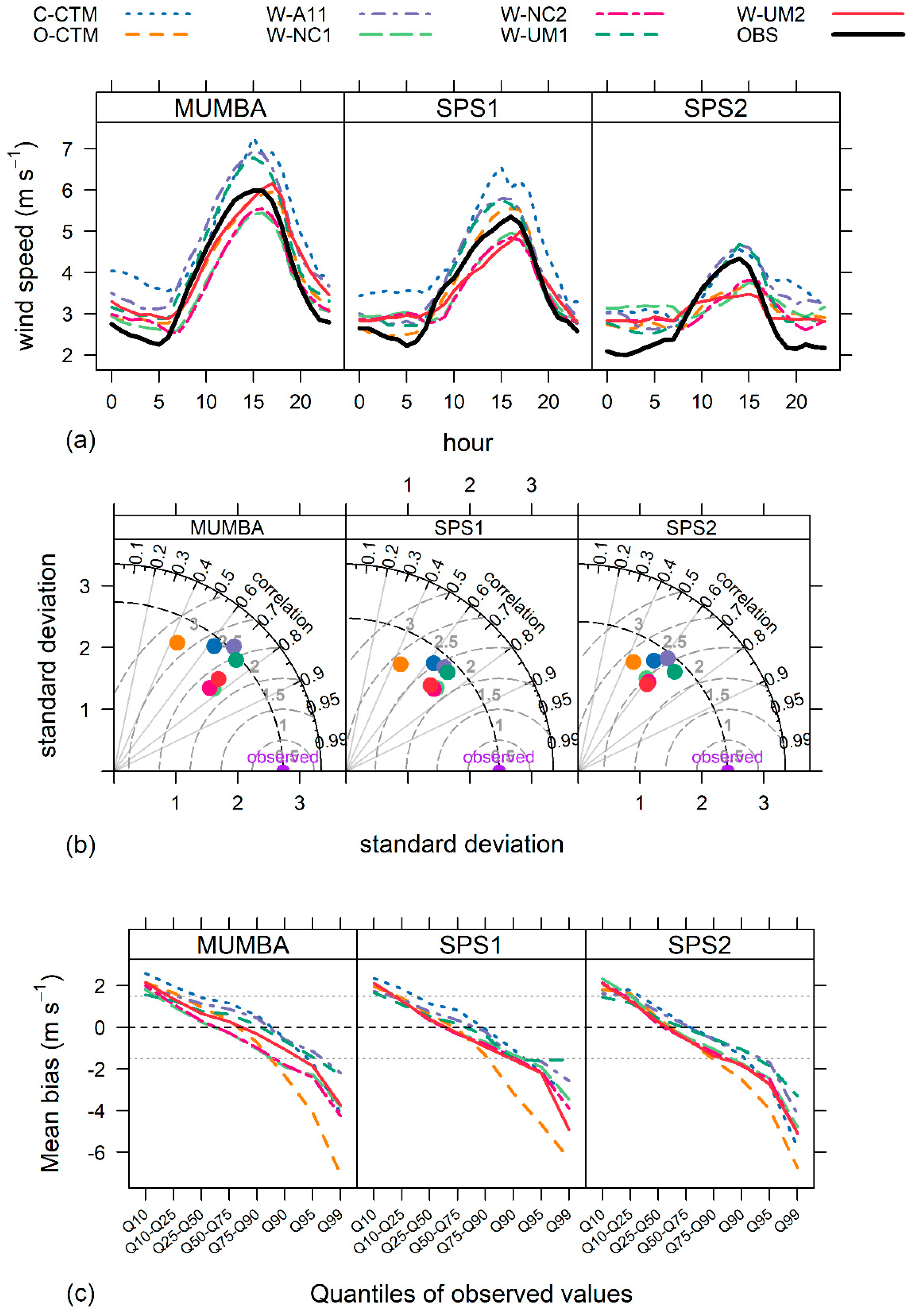
The composite diurnal plots are followed by a panel of Taylor diagrams summarising model performance in terms of standard deviation, correlation coefficients and centred root-mean-square error (CRMSE) for each campaign. On the Taylor diagrams the standard deviations of the hourly observations are indicated with a dashed radial line and the point of perfect agreement with observations is marked as ‘observed’ on the x axis. The strength of the correlation between modelled and observed hourly variables are indicated by the Pearson’s correlation coefficient (R) shown on the outside arc. Finally, the CRMSE is indicated by concentric dashed grey lines emanating from the ‘observed’ value. The last panel presents mean bias (MB) for paired model/observed values, split into quantile bins (0–1, 1–5, 5–10, 10–25, 25–50, 50–75, 75–90, 90–95, 95–99 and 99–100 percentiles) of observed values. Tables of the statistics are presented in the Supplementary Material (Tables S1–S5).
To investigate how each meteorological model performs through the atmosphere we also examine radiosonde observations (released twice daily from Sydney Airport at approximately 6:00 (morning) and 15:00 (afternoon) local standard time—UTC+10). Both the observed and model profiles are interpolated to the altitudes of 20, 50, 100, 150, 250, 500, 750, 1000, 2000, 3000, 4000 m above ground level. The focus of this study in on the lower 4000 m of the atmosphere as it is most relevant for air quality modelling, however, the full profile up to 20,000 m elevation can be found in the Supplementary Material (Figures S4, S6 and S8). The statistical metrics (MB, CRMSE and R) are calculated for temperature, water mixing ratio and wind speed in the vertical. Only the average vertical profiles of the zonal wind component are shown, as the interpretation of the statistics computed on the wind components is difficult due to the positive/negative nature of the data.
The most commonly referenced meteorological benchmarks were established by [69]. The modelling conducted by [69] was over the eastern and mid-west of the US where the terrain is considered flat and “simple”. For more complex terrain the benchmarks provided by [71] and [72] may be more appropriate and are also provided in Table 3. Both the Sydney basin and Wollongong region would be considered complex due to the surrounding ranges/escarpment and the presence of the coastline; therefore, the complex benchmarks will be considered.

3. Model Evaluation Results and Discussion

The following results and discussion sections are based on the hourly averaged data across the seven selected BoM weather stations in Sydney and Wollongong. Box and whisker plots of the MB, R and CRMSE for each model (presented in Figure S1 in the Supplementary Material) highlight some of the variability in the meteorological data across the seven sites. Generally, the average of the seven stations capture the sign and magnitude of the statistics. There appears to be less variability between sites for temperature and water mixing ratio, with the exception of a couple of stations. There is more spread in the statistics across sites for the wind.

3.1. Temperature

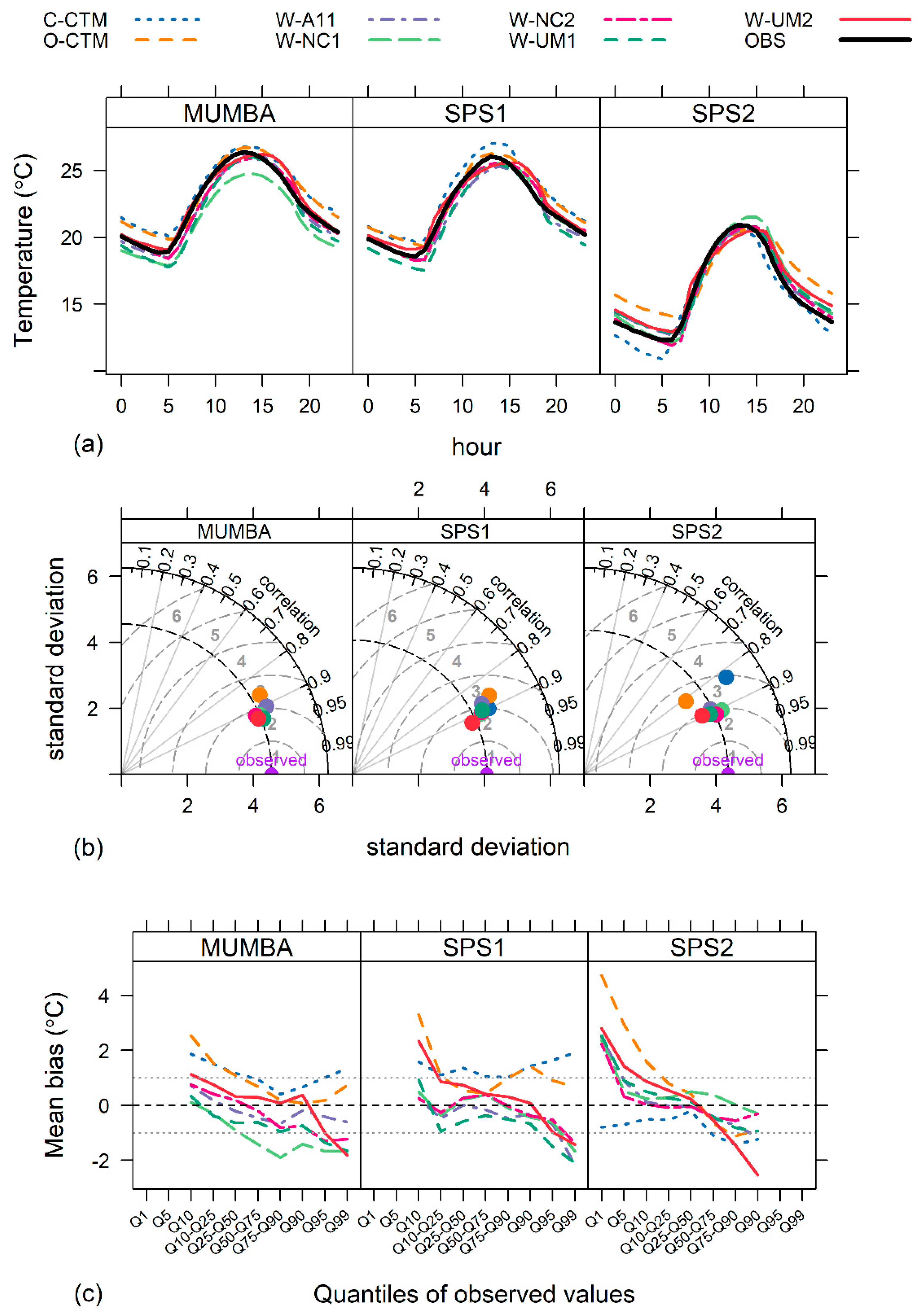
Temperature plays an important role in air pollution due to the temperature dependency of photochemical and aerosol processes, as well as vertical dispersion from buoyancy due to the heat island effect. The WRF 2 m temperatures and the CCAM 10 m temperatures were used for the near surface temperature evaluation. This is the temperature parameter that has been historically evaluated for the CCAM-CTM system [6,72]. The composite diurnal pattern (Figure 2a) is captured by the simulations and the expected shift in temperature between summer (MUMBA/SPS1) and autumn (SPS2) is observed.
There is close agreement between the WRF simulations and the observations, with a small negative bias in the first half of the day across all campaigns. The largest negative bias in the diurnally averaged temperatures is seen in the W-NC1 simulation during MUMBA and W-UM1 during SPS1. The nocturnal temperatures are underpredicted by most WRF configurations during the two summer campaigns and overpredicted during SPS2 (autumn). The O-CTM and C-CTM simulated near surface daytime temperatures during all campaigns are close to the observations. These CCAM simulations overestimate overnight temperatures during all campaigns, except for the C-CTM simulation during SPS2 where they are underestimated.
Taylor diagrams for temperature (Figure 2b) provide a visual comparison of each model’s performance, highlighting in this case a tight clustering of skill between the simulations across all campaigns. The two CCAM configurations are outliers with poorer performance during SPS2. The CCAM models CRMSE range between 2 and 3 °C and tend to have a higher amplitude of variation than the observations, with the exception of O-CTM during SPS2 which is lower. The WRF simulations temperatures are close to the amplitude of the standard deviation for all campaigns with a CRMSE around 2 °C. Overall the correlation coefficients are high (close to 0.9), with the two CCAM simulations slightly lower (around 0.8) during SPS2.
Figure 2c presents the mean bias of the paired modelled and observed hourly averaged temperatures by quantile of observed values. For the WRF model configurations, the bulk of the modelled temperatures (within quartile 25–75) fall within the benchmarks of ±1 °C (denoted by the dashed lines). At the higher and lower ends of the temperature ranges, where there are fewer occurrences, the mean bias is above the benchmark but it remains within ±3 °C of the mean. There is a consistent pattern between all WRF model configurations and across all campaigns of a positive bias for cooler temperatures (too warm) and a negative bias for warmer temperatures (too cool). The two CCAM simulations temperature biases are positive across all quantiles for the summer campaigns, while C-CTM simulation temperature biases are negative during SPS2. During SPS2 the WRF simulations tend to have a larger positive bias in the cooler temperatures compared to the summer campaigns. These biases are seen in the diurnal plots (Figure 2a), particularly overnight when temperatures are at their coolest. Quantile-quantile plots (Figure S2 in the Supplementary Material) show that these biases are not a function of the timing of the temperature variations as they are seen in the unpaired analysis. The greatest deviations from the observations in the WRF simulations are the cooler biases in W-NC1 (MUMBA), W-UM1 (SPS1) and W-UM2 (SPS2), which all remain warmer than −2.5 °C.
The C-CTM and O-CTM simulations consistently overestimate temperatures during the summer campaigns, however, most of these remain within the benchmark values (±1 °C). Similar to the WRF simulations, the CCAM simulations cooler temperatures have a positive bias (up to 3 °C), seen as an overestimation of overnight temperatures in the diurnal plots (Figure 2a). Conversely, the C-CTM simulation underestimate temperatures (but within the benchmark values) during SPS2 and only just beyond the benchmark values for warmer temperatures.
In the daily analysis (Figure S3 in the Supplementary Material) most of the simulated temperatures are close to the observed. These plots show similar biases as seen in the hourly analysis (Figure 2); for example, the CCAM simulations overpredict temperatures by up to 2 °C during the summer campaigns. The performance metrics are improved when considering daily averages, with correlation coefficients above 0.9 for all models. The majority of the mean bias daily temperature quantiles follow the same pattern as the hourly and fall within the benchmark values. The magnitude of temperature biases that are outside the benchmark values are only up to 2 °C.
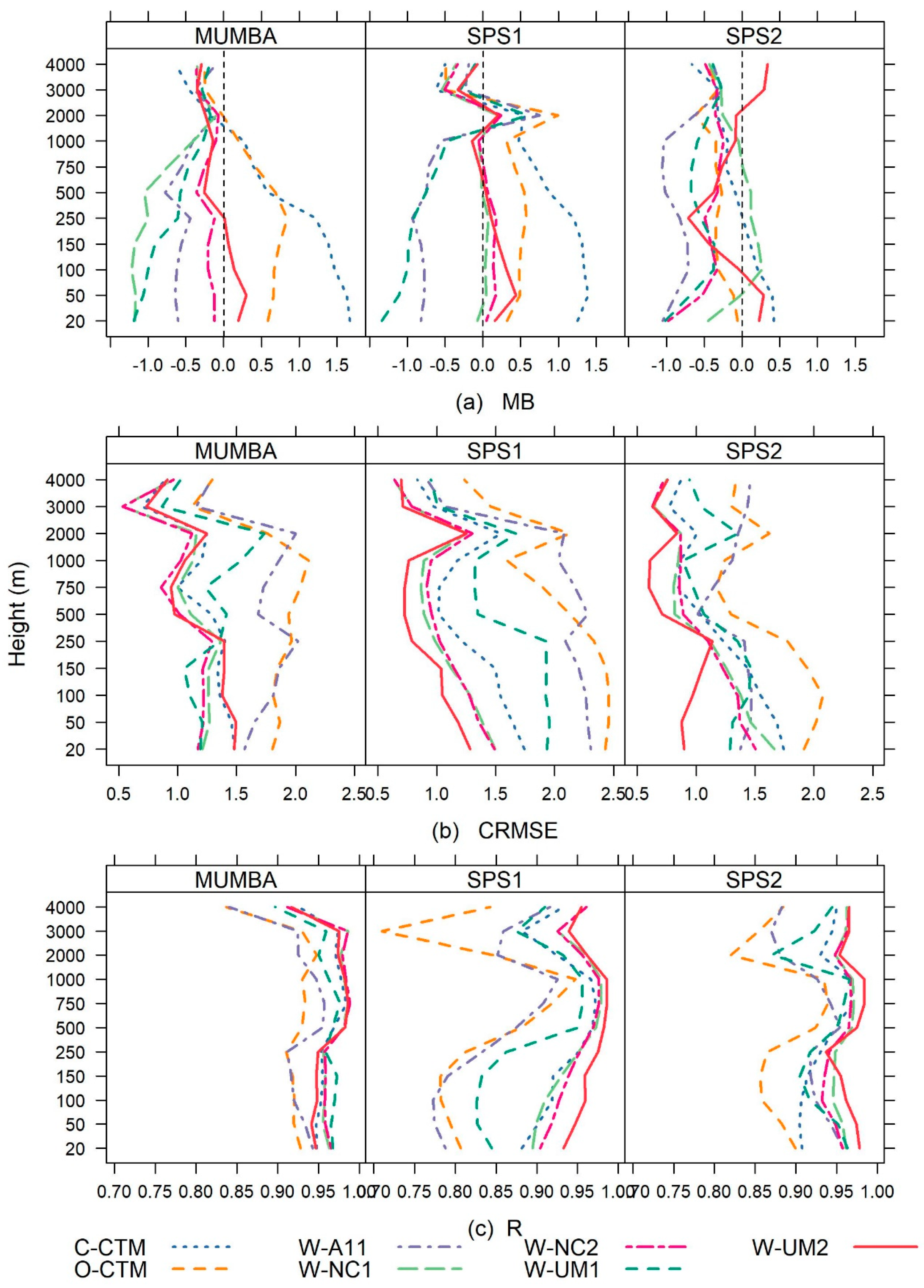
To examine the model performance above the surface, vertical profiles of temperature MB, CRMSE and R at Sydney Airport are presented in Figure 3. Below 4000 m, temperature MB varies between ±1.7 °C for all models. The W-A11 and W-UM1 configurations consistently underestimate temperatures below 2000 m. During SPS1 and MUMBA, the MB for W-UM2 and W-NC2 is close to zero, while their MB ranges between −1 and 0.5 °C during SPS2. The MB for W-NC1 changes between campaigns with the largest (<−1 °C) during MUMBA, close to zero during SPS1 and within ±0.5 °C during SPS2. The CCAM models tend to have a positive bias below 1000 m, except during SPS2 where the O-CTM mean bias is negative and C-CTM becomes negative above 250 m. Since all the models are nudged towards the analysis data (ERA Interim or FNL) above the PBL, the temperature bias in the vertical profiles is likely reduced due to an increasing influence from the gridded analysis data forcing. This would lead to improved model performance above the PBL that would vary depending on the type and strength of the nudging. Both W-A11 and O-CTM consistently have larger biases, greater CRMSE and lower correlations compared to other simulations which may be the result of the weaker scale-selective spectral nudging.
The vertical profiles of CRMSE (Figure 3b) show the spread of CRMSE during SPS1 ranges between 0.5 and 2.5 °C in the lower 1000 m compared to 0.5–2 °C for MUMBA and SPS2. The O-CTM and W-A11 simulations consistently have the largest CRMSE in the vertical across all campaigns, whereas W-UM2 and both the W-NC simulations have the smallest CRMSE. The correlation coefficients (Figure 3c) are generally over 0.9 during MUMBA and SPS2. During SPS1 the correlations coefficients are above 0.9, with the exception of W-UM1, W-A11 and O-CTM which have correlation coefficients above 0.75.
At 2000 m through all statistics, most notable in the SPS1 campaign, is a positive MB, an increase in CRMSE and a reduction in the correlation coefficients. Additionally, the correlation coefficients reach a minimum of 0.7 for O-CTM at 3000 m. These reductions in model performance are the result of the model’s inability to accurately capture upper level inversions observed between 2000 and 3000 m on certain days. This would likely be a response to the choice of PBL parameterisations and there is a similar magnitude response between the simulations that use YSU (W-A11, W-UM1) or MYJ (W-UM2, W-N1 and W-NC2) PBL schemes. It appears that the simulations using the MJY PBL scheme have a greater skill capturing these upper level inversions.
The WRF simulations temperature estimates across all three campaign periods have mean biases at the surface mostly within the benchmark values (±1 °C) and between −1.5 °C and 0.5 °C through the vertical. Pairings of model performance for temperature are seen between W-A11 and W-UM1, which share the same PBL, radiation and LSM physics parameterisation schemes. These two simulations have a tendency for cooler temperature biases that extend through the atmosphere. Comparison between the two W-NC simulations show an improvement in temperature predictions in the lower atmosphere by the inclusion of the ROMS SSTs and further analysis of these two simulations can be found in [49,50].
The CCAM simulations are another pairing which have near surface warm temperatures biases that are largest overnight and greater than the benchmark values (up to 5 °C). The warm temperature biases in the CCAM simulations may be a result of the choice of LSM and its inputs, providing biased surface temperature and moisture. The Community Atmosphere Biosphere Land Exchange (CABLE) [73] is an alternative LSM available to the CCAM system. A recent intercomparison including CCAM run with CABLE LSM [74] had cold maximum temperature biases around ±2 °K and minimum temperature biases around ±1.5 °K over southern Australia, indicating that this choice might lead to improved temperature biases.
Ozone pollution events tend to occur at the peak of diurnal temperatures during summer months. The overestimation (underestimation) of temperatures in the 90th percentile by the CCAM (WRF) simulations suggests that these models may overpredict (underpredict) such episodes.. The larger CRMSE values (>2 °C) indicate that the models could potentially drive large errors in the subsequent air quality modelling, as the largest errors tend to occur during hotter days when photochemical activity is more likely. The impacts of these biases on ozone predictions are discussed further in [33].
The cooler nocturnal temperatures, seen predominantly in the W-UM1 and W-NC1 simulations during SPS1 and the C-CTM simulation during SPS2, could potentially be associated with more stable/calmer nights and reduced dispersion (see Section 3.4). The evaluation method discussed in [8], enables a closer, separate investigation of conditions at the extreme ends of the scale. They found the nocturnal temperature estimates in the models showed a strong sensitivity to stability class, with the poorest performance seen on the most stable nights. They also found the largest variability in model skill was under the most stable nocturnal conditions (associated with clear sky days the following day) and the best skill was during well mixed conditions. It should be noted that this analysis was focused on autumn (SPS2) only.

3.2. Mixing Ratio of Water

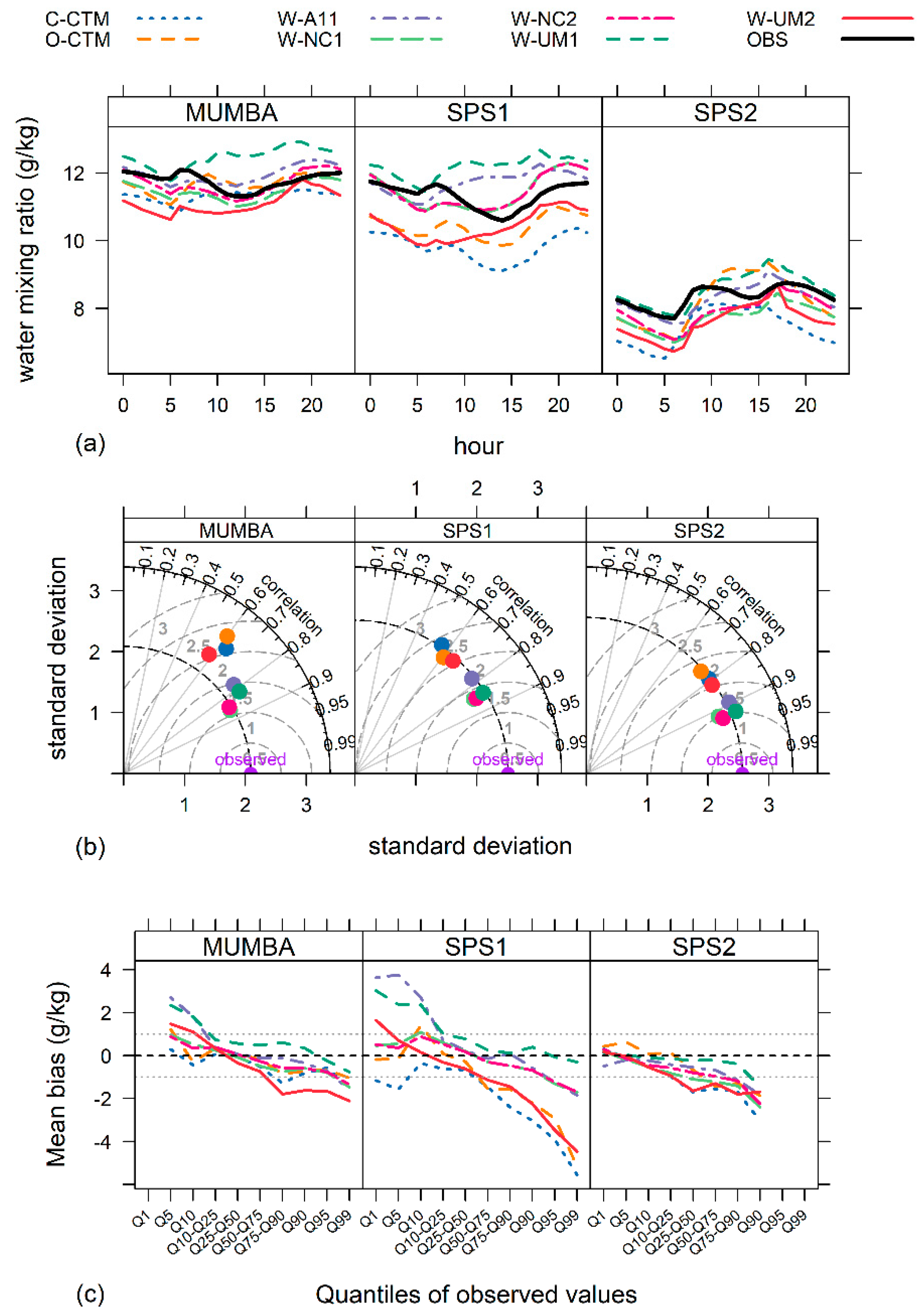
Moisture in the atmosphere influences both photochemistry and aerosol formation. There is no clear diurnal cycle in the mixing ratio of water, as seen in Figure 4a. The models capture the seasonal change between the drier autumn months of SPS2 and higher moisture in the two summer campaigns. Most models underestimate water mixing ratio, with the largest deviations overnight. W-UM2 is consistently drier than the observations across all campaigns. Conversely, W-UM1 consistently overestimates water mixing ratio throughout the day across all campaigns, while W-A11 and both the W-NC models overestimations predominantly occur after 10:00 local standard time (UTC+10). The CCAM models are drier during the SPS1 campaign and O-CTM is wetter on average than observations during the daytime for MUMBA and SPS2.
The Taylor plots in Figure 4b all show a dispersed model performance for water mixing ratio. The best performance is seen for the W-NC models and W-UM1, with the poorest performance for W-UM2 and the CCAM configurations. The variability of the models tends to be greater than the variability of the observations during MUMBA. This was not observed for the SPS campaigns where the variability of the models was the same or slightly less than the variability of the observations. The driest models (O-CTM, C-CTM and W-UM2) have CRMSE between 2 and 3 g/kg for the summer campaigns and 1.5–2 g/kg for SPS2, while for the other WRF simulations the CRMSE was between 1 and 2 g/kg. The correlation coefficients generally range from 0.6 to 0.95, except for C-CTM during SPS1 which had a lower correlation coefficient around 0.5.
The paired quantile mean bias plots for water mixing ratio (Figure 4c) highlight that the biases of the extreme dry measurements are too wet (positive mean bias) and for the high water vapour measurements the simulations are too dry (negative mean bias). The majority of the data sits within the benchmark values (±1 g/kg). The largest underestimation of surface moisture (between −4 and −2 g/kg) is seen in W-UM1, C-CTM and O-CTM simulations during SPS1.
For daily averages (Figure S5 in the Supplementary Material), there is an improvement in the model skill with smaller differences between simulated and observed water mixing ratios. The correlation coefficients are above 0.8 for WRF simulations and between 0.6 and 0.9 for both CCAM simulations.
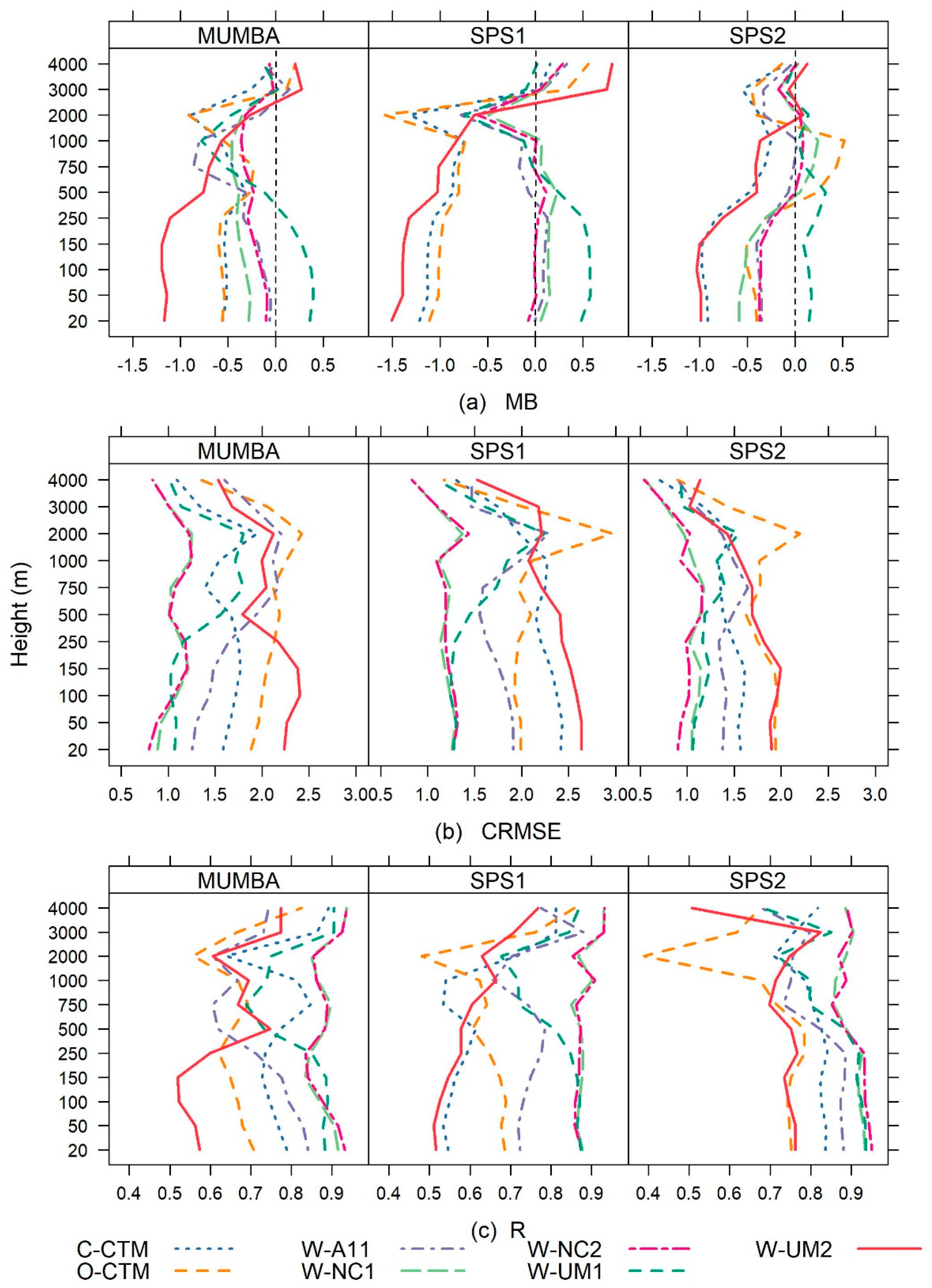
Figure 5a shows that the MB of water mixing ratio throughout the vertical profile is underestimated by most models at the BoM Sydney Airport site. A small positive MB (<0.6 g/kg) is observed in the lower levels of the W-UM1 simulation during all three campaigns, and the W-NC1 and W-A11 simulations (<0.2 g/kg) during SPS1. The W-UM2 simulation below 2000 m had the largest negative vertical moisture MB (between −1.5 and −1 g/kg) for all three campaigns. The CRMSE (Figure 5b) ranged between 0.5 and 3 g/kg across all campaigns. Above 1000 m the variability of CRMSE between simulations decreases and tends towards zero, which again may be a function of the analysis nudging above the PBL. The correlation coefficients (Figure 5c) are similar to those at the surface, between 0.4 and 0.95. The spread between models during SPS2 is smaller, with higher correlation coefficients (>0.7).
Overall the water mixing ratio from the simulations of these three campaigns fall within the benchmark values (±1 g/kg). Similar to temperature, there are pairings of model performance. The W-A11 and W-UM1 simulations have a tendency to be too moist. The W-NC simulations have the smallest biases, however, unlike with temperature, the differences between the two simulations are small, indicating that the addition of the ROMS has less of an impact on atmospheric moisture. The CCAM simulations tend to be too dry, along with the W-UM2 simulation. All performance statistics, both at the surface across Sydney and through the vertical at Sydney Airport, are consistently better during SPS2 compared to the summer campaigns.
Again, a notable feature appears at 2000 m where there is an increasingly negative spike in the MB. This dry MB is largest for SPS1 CCAM simulations and is aligned with the warm temperature biases seen in Section 3.1. These warm, dry biases, where the variability of each of the model simulations are increased and the correlation coefficient are reduced, is the result of the model’s inability to accurately capture upper level inversions observed between 2000 and 3000 m on certain days.
Perhaps as expected, the simulations tend to overestimate moisture during relatively dry observed conditions and underestimate moisture during relatively moist observed conditions. The underestimation of atmospheric moisture, particularly in the W-UM2 simulations during all campaigns and the CCAM simulations during SPS1, could result in impacts on subsequent air quality modelling. In particular they may result in reductions in afternoon convection or formation of non-precipitating cloud which could alter solar radiation, chemistry and secondary aerosol formation.
The possible sources of these drier conditions in the CCAM simulations may be from soil moisture and temperature biases from the LSM, similar to what may be driving the temperature biases seen in Section 3.1. Additionally, accurate soil moisture is achieved with a multi-year spin-up time [75], however, the longest spin-up in these simulations was one month in C-CTM and the shortest was two days for W-UM2. Increasing the length of the spin up of the LSM may result in improved surface fluxes and, subsequently, temperature and atmospheric moisture.

3.3. Wind

Winds influence the spatial distribution and concentrations of pollutants through processes of dispersion, advection and turbulent mixing. It is, therefore, critical to accurately characterise the air flow speed and direction for input into air quality models. Statistical comparisons of wind speed measurements are straightforward, however, there is a relationship between model skill and the wind speed when considering wind direction [76]. Jiménez et al. [76] found large differences between simulated and observed winds at low wind speeds and in complex terrain, while the inverse was found for higher wind speeds and flatter terrain. Comparisons of wind direction will not be examined in this evaluation, however, it is interesting to investigate how well the models capture the strong afternoon north-easterly sea breeze that is critical for ozone formation and transport in the Sydney region [26]. Given that the predominant feature of the sea breeze is the east-west wind component, this evaluation will focus on the zonal winds. The meridional wind plots can be found in Figures S10 and S11 in the Supplementary Material.

3.3.1. Wind Speed

On average all the models overestimated nocturnal wind speeds during all three campaigns (see Figure 6a), with the exception of O-CTM during SPS1. During the daytime throughout the two summer campaigns, C-CTM, W-A11 and W-UM1 all overestimated wind speeds on average. During SPS2 these three models simulated average daytime wind speeds closer to the observations. The other three WRF configurations (W-UM2, W-NC1 and W-NC2) all underestimated wind speeds during the day across all campaigns. O-CTM overestimated daytime wind speeds during SPS1, getting close to observations on average during MUMBA and underestimating on average during SPS2.
There are two clusters of wind speed model performance in the Taylor plots (Figure 6b), aligning with the above mentioned diurnal groupings (W-A11, W-UM1 and C-CTM in one cluster and W-UM2 and both the W-NC simulations in the other). All models show lower variability than observed and this deviation is largest for W-UM2 and both the W-NC models in all three campaigns. The correlation coefficients range between 0.5 and 0.8 for the SPS2 campaign and 0.6 and 0.8 for the summer campaigns. The O-CTM is an outlier with a correlation coefficient close to 0.4 for all three campaigns.
The quantile plots of the paired wind speed mean bias (Figure 6c) show that the lower 10% (Q10) of wind speeds tend to be overestimated (too fast) and the higher 10% (Q90) of winds speeds are underestimated (too slow). The bulk of the wind speed biases are within the benchmark values (±1.5 m s−1) and the largest biases are seen in the higher wind speeds. The largest negative biases are seen for the O-CTM (over −6 m s−1), W-UM2 and both the W-NC simulations (up to −4 m s−1), which corresponds with the underestimation of daytime wind speeds seen in Figure 6a. The exception to this is O-CTM during SPS1. This simulation overestimates peak daytime wind speeds on average (Figure 6a); however, the lower correlation and the larger negative mean bias when the winds speeds are fastest, suggests this simulation has the poorest performance across this campaign.
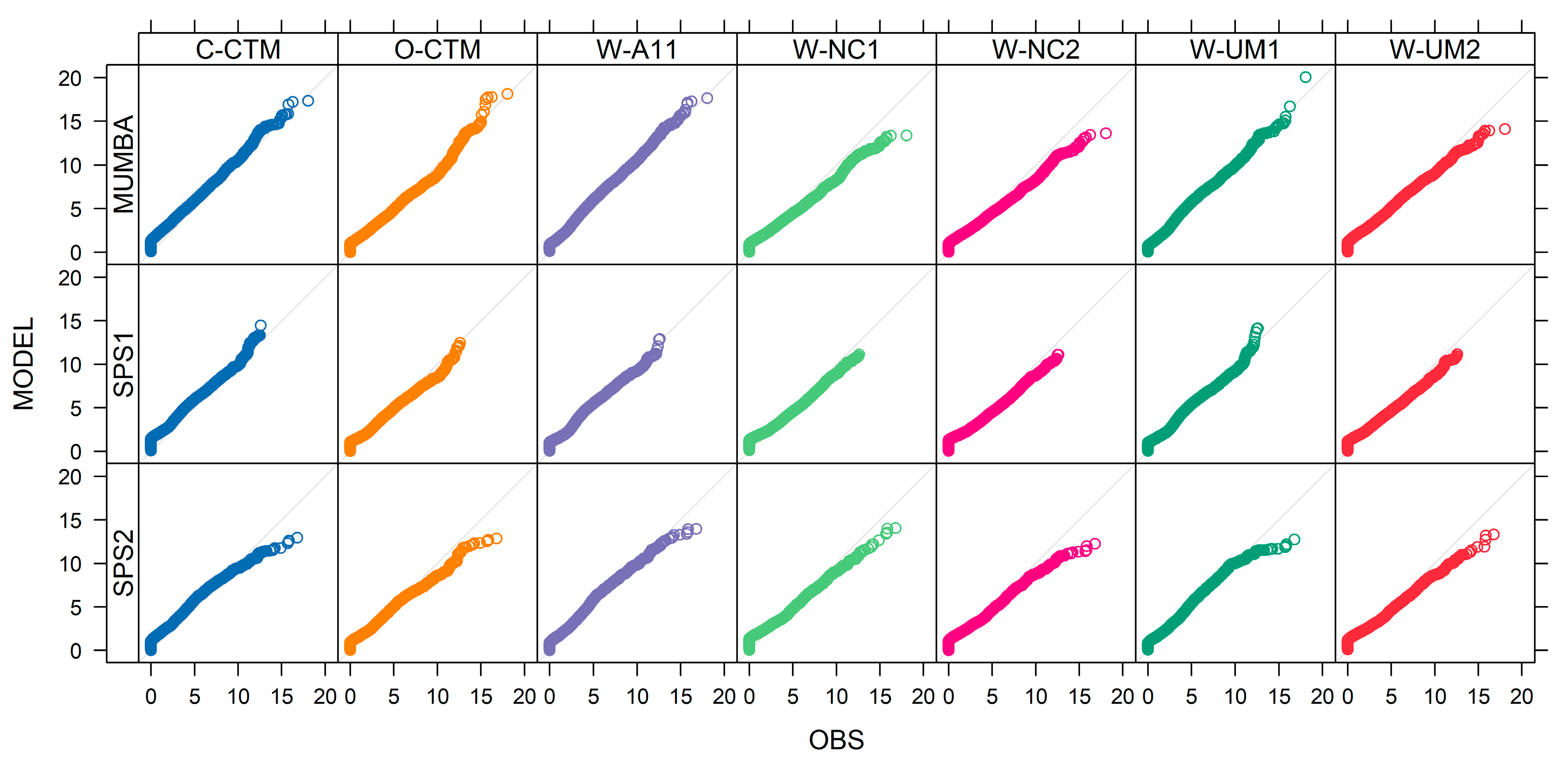
Examining the quantile-quantile plots (Figure 7), most of the models underestimate the highest wind speeds, agreeing with the paired mean bias plots (Figure 6c). During MUMBA W-UM1, and to a lesser extent W-A11 and the CCAM models, overestimate the high wind speeds, in particular around 15 m s−1. This overestimation is also seen in SPS1 for C-CTM, W-A11 and W-UM1. This differs from the paired mean bias plots (Figure 6c), suggesting that these models have disproportionately high wind speeds overall compared to the observations and the timing of the modelled high wind speed events does not coincide with observed events.
The daily analysis (Figure S7 in the Supplementary Material) shows that the wind speeds are overestimated on this time scale. The Taylor plots highlight overall better model performance in the daily analysis compared to the hourly. The daily averaged correlation coefficients compared to the hourly averaged analysis increase to 0.6–08 for W-A11, W-UM1 and O-CTM, while all other model simulations correlation coefficients were greater than 0.8. For daily averages the wind speed mean biases all lie within the benchmark values.
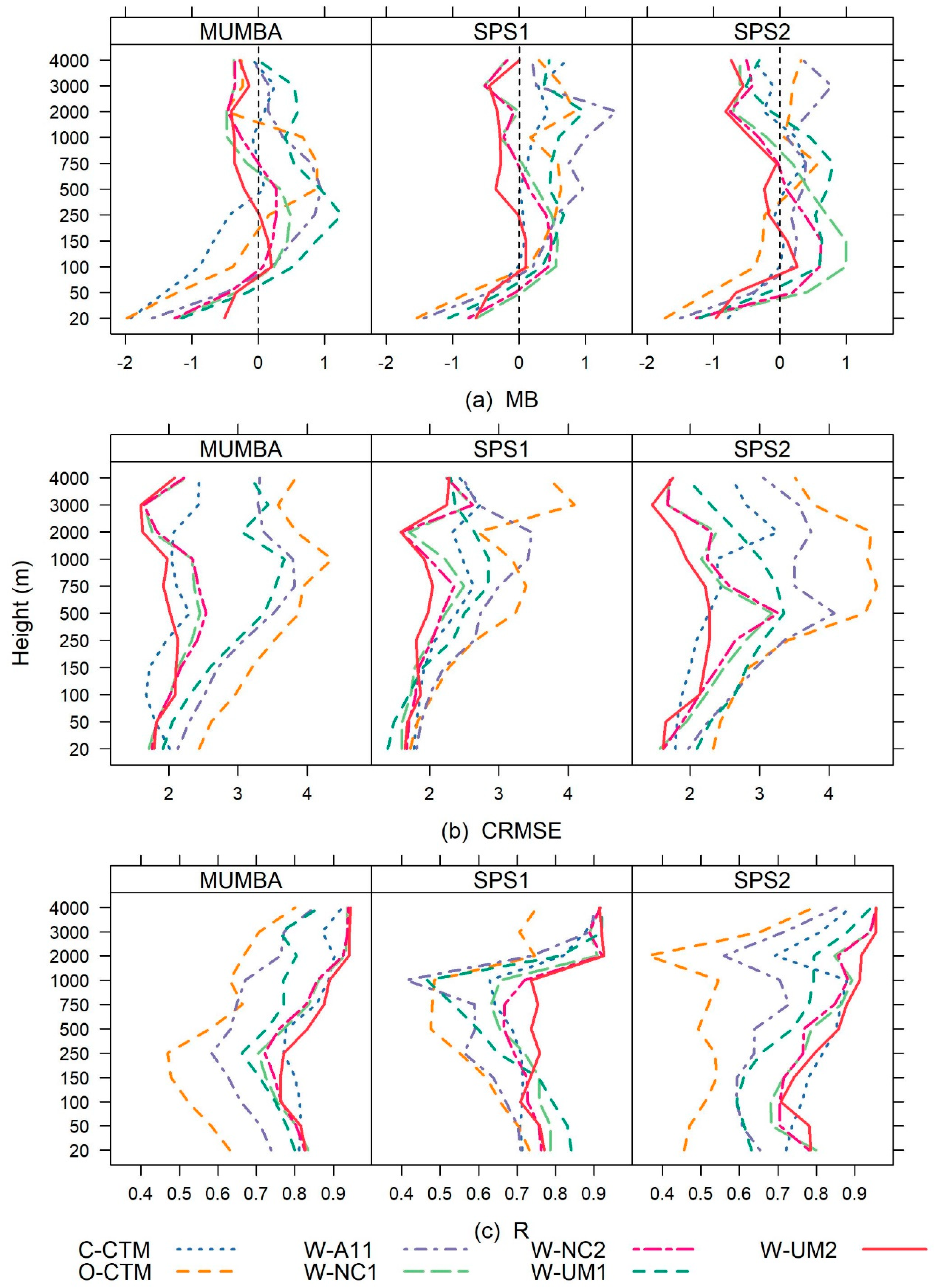
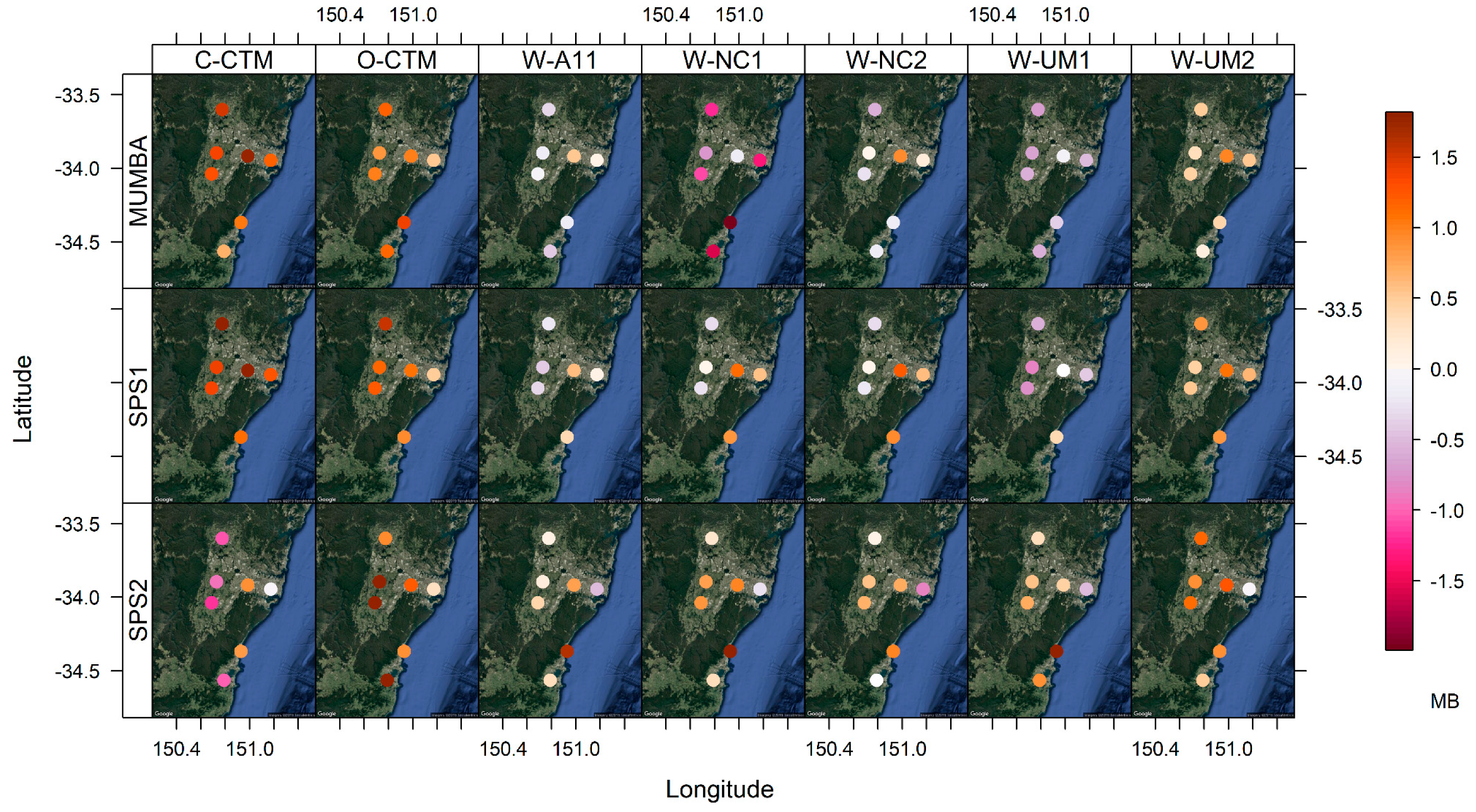
Overall the mean biases in the vertical (Figure 8a) are within the benchmark values (±1.5 m s−1), becoming smaller (within ±1 m s−1) above 1000 m, with the exception of the C-CTM and W-A11 simulations at the surface during MUMBA. The negative bias for all models in the lowest levels (Figure 8a) differ from the surface analysis (Figure 6), with positive biases overnight for all simulations in and the W-A11, W-UM1 and the C-CTM simulations during the day. This difference is due to the vertical profiles only containing BoM Sydney Airport data, where the wind speeds are, on average, higher due to its location close to the coast. The models tend to underestimate winds at this site. This is seen clearly in the bubble plot of surface mean bias in Figure 9, where the mean bias is negative at Sydney Airport and often at another coastal site further south, whereas the mean bias is positive at all other sites.
The CRMSE (Figure 8b) is similar among the models, with values between 1.5 and 4 m s−1. The correlation coefficients (Figure 8c) are generally greater than 0.6 for MUMBA and SPS2. In the SPS1 simulations the correlation coefficients decrease from 0.80 to a minimum of 0.4 at 1000 m, particularly in the O-CTM, W-A11 and W-UM1 simulations. This reduction in correlation at 1000 m is the result of these simulations overestimating the wind speeds over several days. The improvement in model performance above the PBL is again potentially due to the nudging above the PBL forcing the models towards the gridded analysis data (ERA-interim or FNL).

3.3.2. Winds Components

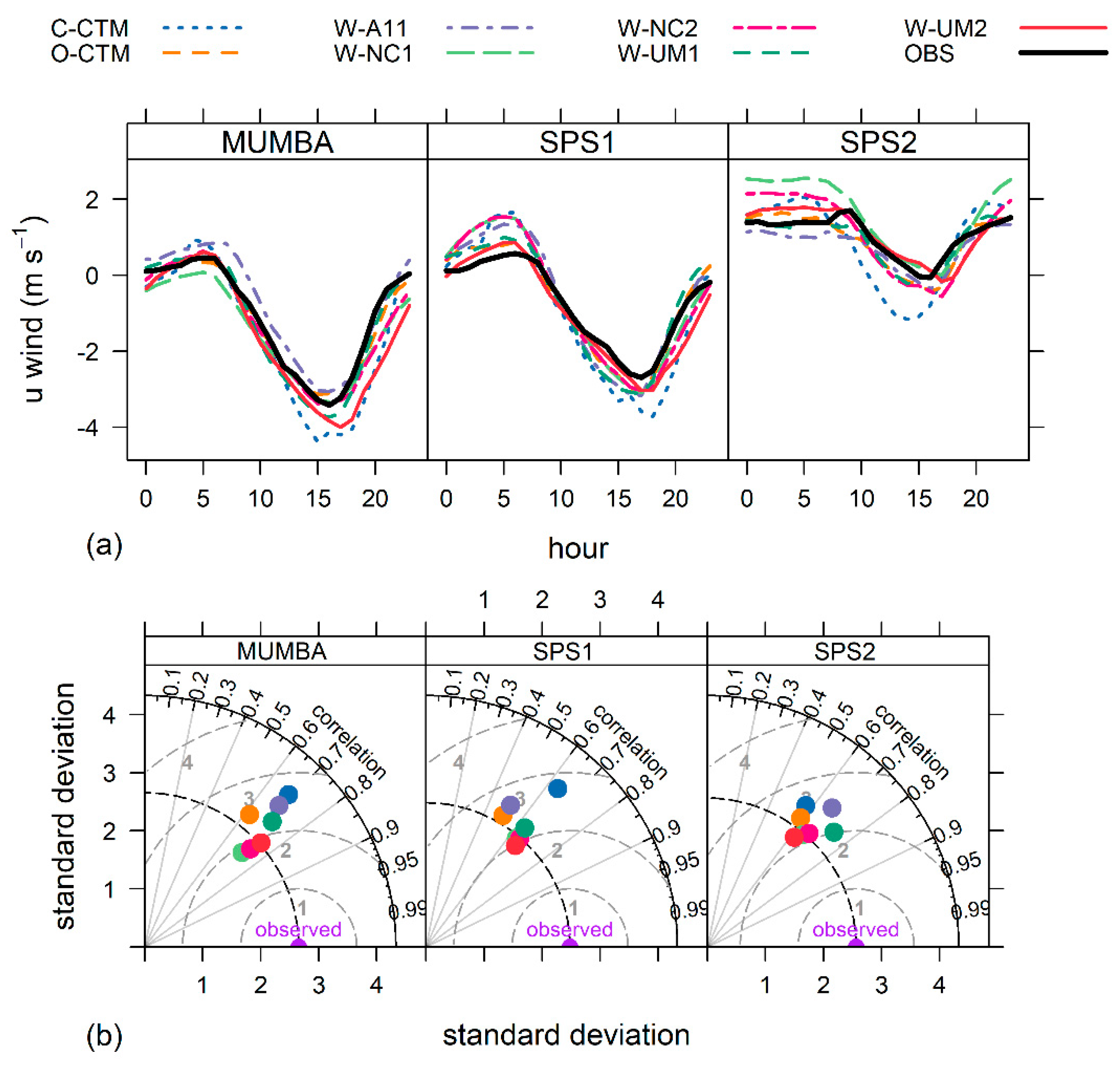
The strong sea breeze that occurs predominantly during summer is seen in the diurnal plots of zonal winds (Figure 10a), with the models showing good agreement with the observed average diurnal cycle. The easterly wind component peaks around 3 pm during the summer campaigns (SPS1 and MUMBA) and all the models on average capture this feature. During SPS2, the westerly component dominates with a weaker easterly shift than the observations on average by 4 pm. The amplitude of the shift from westerly to easterly in the diurnally averaged plots is larger than observed for almost all models. The C-CTM has the largest deviation from the observations during all campaigns.
Model performance of the zonal wind components vary considerably, particularly during the summer campaigns, as illustrated by the spread in the Taylor plots (Figure 10b). Both the W-NC simulations and W-UM2 are clustered together with slightly lower variability than the observations, whereas W-UM1, W-A11 and both the CCAM simulations have higher variability than the observations. This is similar to the Taylor plots for wind speed (Figure 6b). The correlation coefficients range between 0.5 and 0.8 for all campaigns.
The analysis of daily averaged zonal winds (Figure S9 in the Supplementary Material) shows a similar level of performance for MUMBA and SPS2 and decreased performance for SPS1. Interestingly, the performance seen in the Taylor plots of the daily averaged meridional winds (Figure S11b in the Supplementary Material) is improved when compared to the hourly analysis, as the north-south component of the winds is more likely a synoptic feature and better captured on daily time scales. However, the local sea breeze is a diurnal feature which is better represented by the hourly analysis.
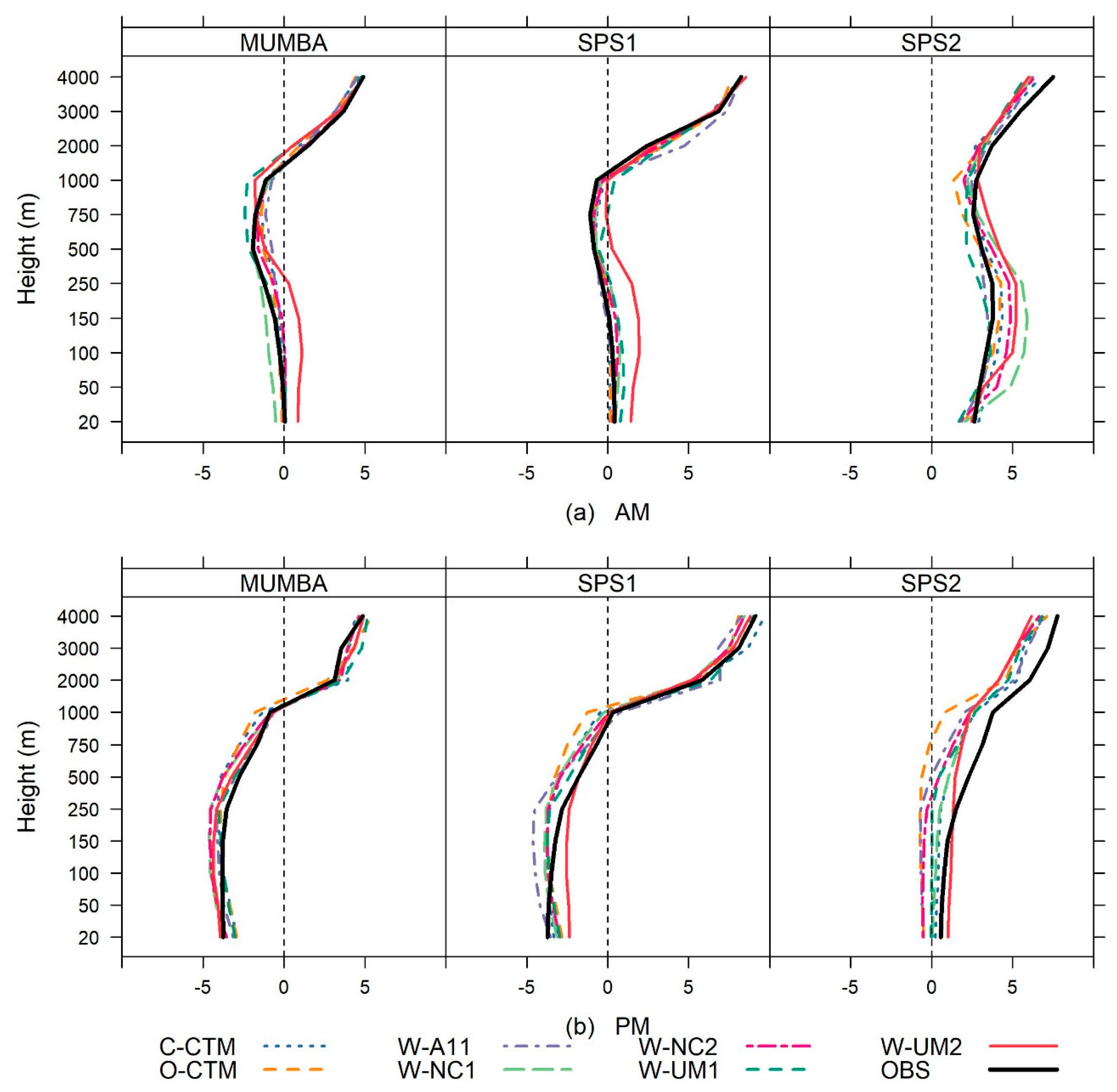
The averaged zonal wind through the vertical profile for the morning (AM) and afternoon (PM) soundings are presented in Figure 11a,b. Overall the models tend to follow the observed average wind component through the vertical, with a weak westerly component (positive) in the morning during summer, easterly (negative) at the top of the boundary layer and westerly (positive) above the PBL. In the afternoon the sea breeze has set up an easterly wind flow within the PBL and the westerlies remain above. During autumn (SPS2), the winds are consistently westerly through the vertical profile in the morning. The afternoon winds generally remain westerly, however, the strength is much less in the O-CTM, W-A11 and W-UM1 simulations, where the lower 1000 m has a slight easterly component.
The consistent overestimation of calm nocturnal wind speeds seen in all simulations, could lead to an underestimation of pollutant concentrations due to unrealistic dispersion. These calm conditions are important for air quality as they are generally associated with high pollution events. Vautard et al. [11] also saw this overestimation and suggested it may be associated with insufficient vertical resolution and excessive vertical diffusion. Chambers et al. [8] demonstrated this overestimation of nocturnal winds by the models (especially under stable conditions) and linked this problem directly to overestimated PBL depths and found the resultant pollutant concentrations were also underestimated. This overestimation of wind speeds may be due to the assigned surface roughness in the models, the thickness of the near-surface model layer, or a host of challenges associated with modelling the surface boundary layer [77,78] especially under weak winds and strong stratification [79].
Conversely, an underestimation of winds speeds, seen across the daytime of the W-UM2 and both W-NC simulations, may lead to an overestimation of pollutant concentrations as dispersion and advection would be reduced. The difference between coastal and inland wind speed biases could also potentially impact air quality simulations. The models appear to be unable to capture the observed shift in wind speeds between coastal and inland station locations.
In addition to wind speed, predicting the direction that air pollutants are transported is critical to accurately modelling air quality impacts. The models appear, on average, to capture the direction and amplitude of the daily sea breeze, a key component in the formation and transport of ozone across the Sydney basin. In this location, the sea breeze provides a clear demonstration of the importance of accurate wind fields for other meteorological parameters. For example, W-A11 (Figure 11b) develops an overly strong sea breeze and as a result the water mixing ratio has a high bias in the afternoon. The resultant chemical species may then be affected in a similar manner.

3.4. Planetary Boundary Layer Height

Turbulent mixing in the boundary layer of the atmosphere controls the dilution of air pollution at the surface. In order to assess each model’s ability to simulate turbulent mixing, the PBLH has been investigated. Each modelling system provides PBLH, however, the methods for computing it can vary between models. For consistency, the PBLH for both the model output and the observations has been derived using a method based on the bulk Richardson number (Ri), as described in [80]:
Ri ( z ) = ( g / θ v s ) ( θ v z   θ v s ) ( z z s ) ( u z u s ) 2 + ( v z v s ) 2 + ( bu 2 )
The Ri profile is calculated using the virtual potential temperature (θv), wind component profiles (u and v) starting from surface values (denoted by s) of 0 and ignoring surface frictional effects (b = 0). The first level with a Ri ≥ 0.25 is identified and linear interpolation between that level and the next lowest level provides an estimate of the PBLH.
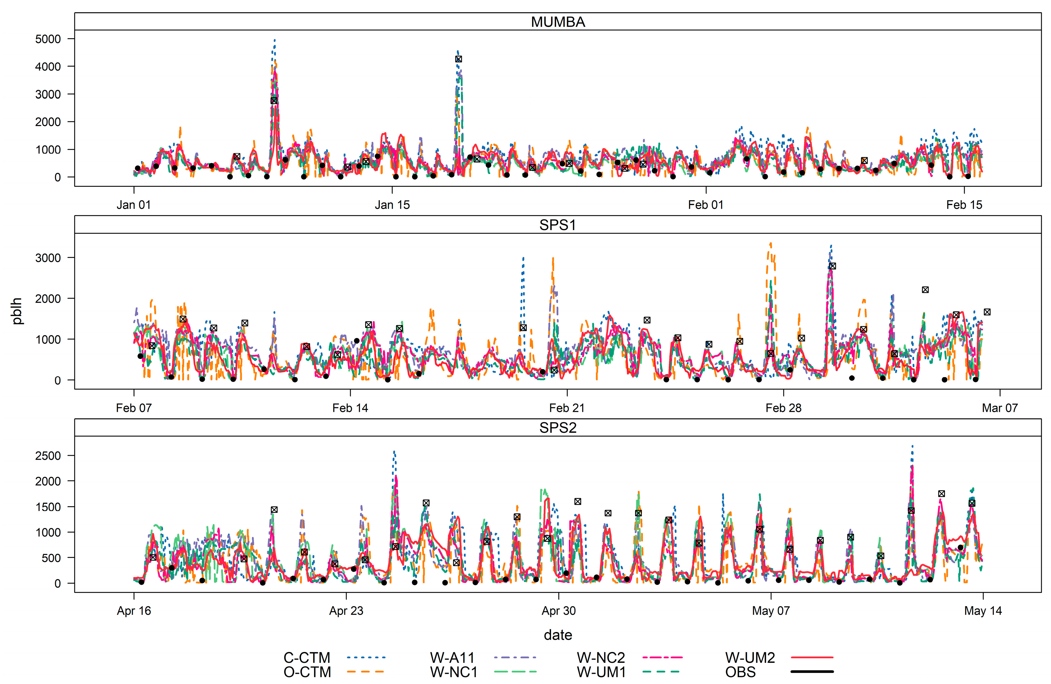
The PBLH is computed for each morning (AM) and afternoon (PM) radiosonde measurement at the BoM Sydney Airport site and are presented in Figure 12 (denoted by black dots for AM and black crosses in a box for PM) along with the full time series of the modelled PBLH. Although the observations are sparse during some periods, it is evident that the model simulations capture some of the day-to-day variability of the PBLH in addition to several anomalous events.
The two hot days in January (8th and 18th) of the MUMBA campaign, when the PBLH peaks above 2000 m during the afternoon, are captured by all models for the first event, but only by W-A11, W-UM1 and the two CCAM simulations for the second event. The timing of the peak is slightly later for the W-UM2 simulation of January 8th, however, the magnitude is closer to observations. All other simulations overestimate the PBLH between 500 m (W-UM1) and 2000 m (C-CTM) on January 8th. There was no recorded rainfall during these two events, so the peaks are associated with heating, not convective rainfall. The improved ability of the W-A11 simulation to capture the deep convection on both hot days may be the result of increased vertical resolution (56 vertical levels), however, the W-UM1 simulation has similar vertical resolution to all other simulations (33 vertical levels).
Both the W-A11 and W-UM1 simulations used the MYJ PBL scheme (local closure) and more accurately simulated the deep convection during the two hot days during MUMBA compared to the simulations that used the YSU PBL scheme (non-local closure). The treatment of localised stability maxima by the YSU non-local closure scheme should allow for a more realistic representation of mixing from large eddies [81], simulating deep convection more accurately. However, it was not the case in our comparison since the MYJ local closure scheme in the W-A11 and W-UM1 simulations were able to simulate the larger PBLH during both of these events. This agrees with what was also seen in [21] and the use of MYJ for this region was recommended in the performance evaluation of WRF simulations over south eastern Australia in [82]. The CCAM simulations employ a non-local closure PBL scheme and appear to simulate the deep convection during these events well.
During SPS1 there were two days towards the end of the measurement campaign (March 1st and 4th) when the observed PBLH was greater than 2000 m. However, these peaks were not associated with above average temperatures. The C-CTM, W-A11, W-NC1 and W-NC2 simulations all captured the amplitude of the first peak, however, none of the simulations captured the amplitude of the second peak. There were also at least two days when some of the simulations overestimated the PBLH up to 2000 m. The large overestimations of the first day (February 20th) were predominantly from O-CTM and W-A11, W-UM1 and W-UM2 and during the second day (February 27th) it was O-CTM, W-UM1 and both the W-NC simulations. During SPS2, there were no days when the PBLH peaked over 2000 m, however, all simulations, except W-UM2, overestimated the PBLH peaks up to 1500 m on two days. There does not seem to be a PBL scheme that performs better during the SPS1 and SPS2 campaigns.
The campaign averaged normalised mean bias (NMB) computed for morning and afternoon observations are presented in Table 4. During the morning, generally all models overestimate PBLH, with the exception of O-CTM during MUMBA. Conversely during the afternoon, the models underestimate PBLH. The exceptions to this are C-CTM, O-CTM and W-A11 during MUMBA when the models overestimate the magnitude of the PBLH on the afternoon of the first of the two hot days. Additionally, W-NC1 on average overpredicts the afternoon PBLH during SPS2.
There is a considerable amount of spread in model performance as seen in the Taylor diagrams of PBLH (Figure 13). It is evident that the model simulations generally overestimate variability in the morning, with the exception of W-UM2 and both the W-NC models during MUMBA and W-UM1 during SPS2. Conversely, the Taylor plots illustrate lower variability in the modelled afternoon PBLH compared to observations for most simulations, except for both W-NC simulations during SPS2 and C-CTM in all campaigns. Overall, correlation coefficients are low, ranging between 0 and 0.6, with the exception of the W-UM1, W-A11 and C-CTM simulations during the afternoon of the MUMBA campaign where the correlation coefficients are over 0.9. This improved performance is the result of better simulating the peak in PBLH associated with the hot days during January of the MUMBA campaign. The poorest performance overall for PBLH is seen during the SPS1 campaign, which seems to be the most challenging campaign to model overall.
The analysis performed here indicates that the models have limited skill in accurately predicting the PBLH. There are two aspects to the PBLH observations which may be behind the errors in the PBLH. Firstly, the observations are effectively discrete points in time, so that apparent biases in the morning PBLH can be caused by errors in the timing of PBL growth. Second, the radiosonde launch site is close to the coast, situated on the shore of Botany Bay and 8 km inland from the ocean. This has the potential for small errors in wind direction to dramatically change the measurements upwind.
Most simulations tend to over predict the PBLH during the morning and under predict the PBLH during the afternoon. The overestimation of the morning PBLH height has the potential to lead to an underestimation of pollutant concentrations due to overestimated turbulent mixing. The overestimated PBLH aligns with the overestimated nocturnal temperatures and wind speeds seen in Section 3.1 and Section 3.3.
The underprediction of the afternoon PBLH would mean reduced daytime mixing and, therefore, potential reductions in dispersion of pollutants. Investigations into PBLH in [8], found that under stable nocturnal conditions there was less variability between the models compared to the unstable categories, suggesting the models inability to accurately model these conditions.

3.5. Precipitation

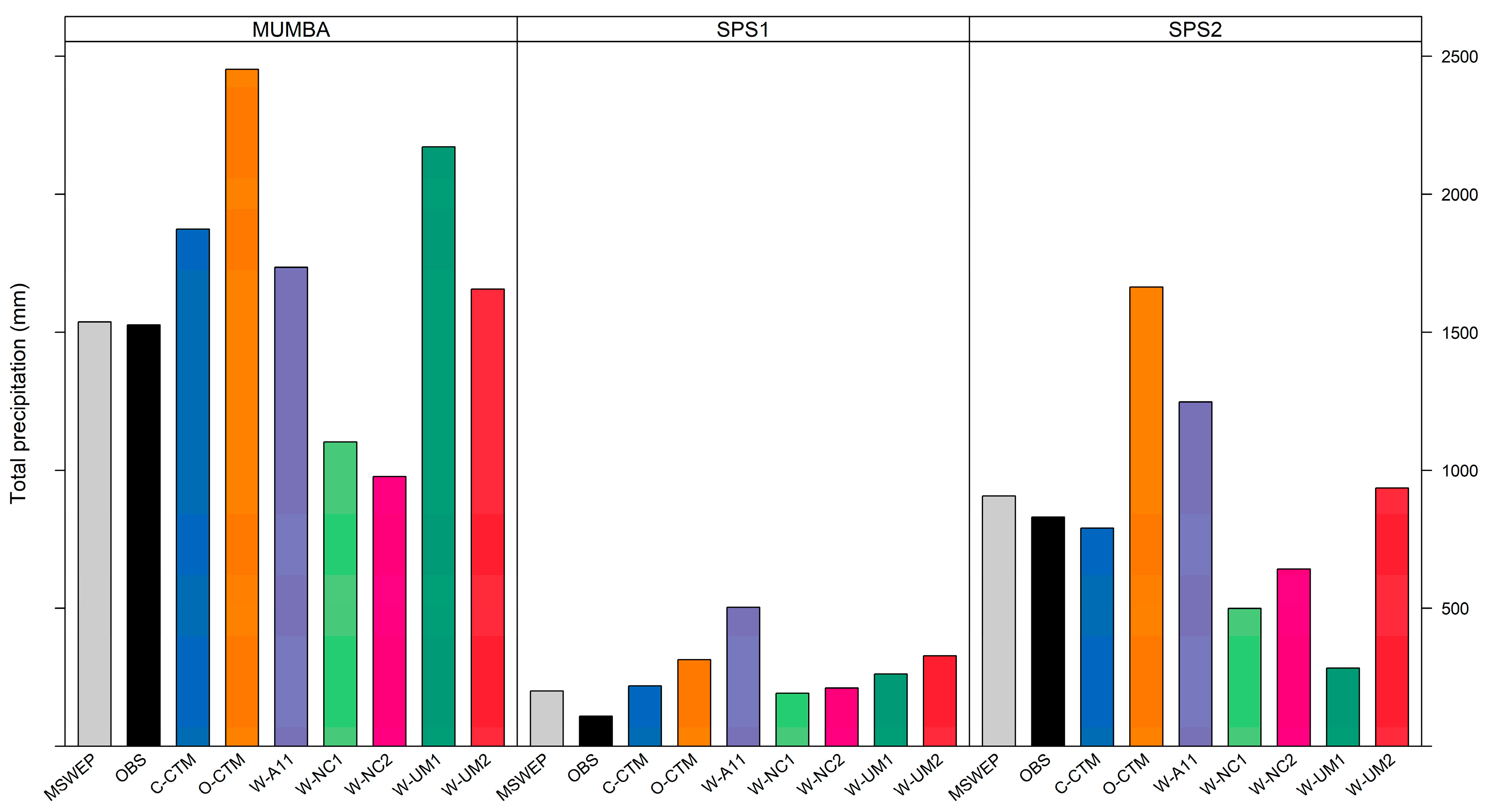
Precipitation impacts air quality predominantly through wet deposition and aerosol scavenging. Figure 14 shows total accumulated precipitation for each model during each campaign compared with the observations and the MSWEPv1.2 gridded precipitation data [83]. Precipitation totals vary by up to 1500 mm between the model simulations and campaigns. Overall, MUMBA had the greatest observed precipitation (occurring at the end of the campaign), while the SPS1 period was relatively dry compared to the other campaigns. The models appear to capture this variability in total precipitation between campaigns, with the exception of a few model simulations.
Total accumulated precipitation modelled during the MUMBA campaign is overestimated by all simulations except W-NC1 and W-NC2. All models have more precipitation than observed during the drier SPS1 campaign, with the W-NC1 and W-NC2 closest to the observations. W-A11, W-UM2 and O-CTM overestimate accumulated precipitation during SPS2 whereas all other models underestimate precipitation for this campaign.
Overall the simulations tend to overestimate total accumulated precipitation. The exceptions are the two W-NC model simulations, which underestimate precipitation during MUMBA and SPS2 as well as W-UM1 during SPS2. The overestimation of precipitation would likely result in underestimation of particulates, while conversely the underestimation of precipitation would lead to an overestimation of particulate pollutant due to reduced wet deposition and aerosol scavenging.
The O-CTM simulation was consistently wetter than the C-CTM simulations which was also seen in the water mixing ratio (Section 3.2). This difference is atmospheric and precipitable water may be the result of different versions of the models (see Table 1). The two W-NC simulations used the MSKF scheme and the precipitation was dominated by non-convective precipitation (analysis not provided in this manuscript), which may explain why these simulations were drier than the other WRF simulations which used the Grell 3D cumulus scheme. The MSKF scheme is relatively new and has proven to have good skill in other regions of the globe, however, this scheme may not be not suited to South-eastern Australia.

4. Conclusions

A model intercomparison has been conducted to evaluate the ability of two meteorological models (CCAM and WRF), used in a suite of seven air quality modelling systems, to reproduce observed features of the local meteorology relevant to air quality and specific to Sydney and Wollongong in NSW, Australia. The modelling covered three periods when air quality measurement campaigns were held to facilitate an in-depth evaluation of the air quality models. The operational evaluation was conducted on hourly data averaged across seven BoM sites, focusing on temperature, water mixing ratio, winds, PBLH and precipitation.
Overall the best performance is seen for the SPS2 campaign (during autumn) when temperatures tend to be cooler, the atmosphere is drier and wind speeds are lower. The data generally sit within the benchmark values, except at either end of the scale, where the bias tends to be larger.
A summary of the findings in this study are:
  • The near surface air temperatures on average are accurately predicted by the WRF models, with biases within ±2 °C and CRMSE <2 °C. There are larger biases (within ±3 °C) and CRMSE up to 3 °C seen in the daytime near surface temperatures in the CCAM simulations. There is a potential for these biases to impact on photochemistry as they do occur when temperatures peak. The largest temperature biases (up to 5 °C) are seen in the nocturnal temperature, which may be associated with the model’s inability to simulate stable conditions overnight and could impact on dispersion in subsequent air quality modelling.
  • Most models show a consistently drier atmosphere than observed, that is largest overnight (<−6 g/kg), while several the WRF simulations overestimate daytime moisture (up to 4 g/kg).
  • The biases in temperature and atmospheric moisture in both CCAM simulations may be the result of biases from land surface fluxes. Further investigations into the ideal spin-up length and choice of LSM may reduce these biases.
  • The wind speeds were consistently over predicted overnight, which is a common issue with meteorological models. The impact of these biases would lead to underestimation of pollutants overnight due to overestimated dispersion/advection. All simulations tend to underestimate the higher wind speeds.
  • The models appear to have the ability to simulate the local-scale meteorological features, like the sea breeze, which is critical to ozone formation over the Sydney Basin. Further analysis into the capability of the models to emulate the progression of the sea breeze front is recommended.
  • The PBLH evaluation highlighted some timing differences in the formation of the PBL, which would likely impact simulated morning dispersion. However, the discrete nature of the observations makes it challenging to fully identify the cause of the biases. Some of the models did better than others at capturing PBLH peaks during MUMBA, with the WRF MYJ PBL scheme showing better performance predicting deep convection during hot days compared to YSU. Neither PBL scheme showed better performance for deep convection not associated with extreme temperatures.
  • Simulated total accumulated precipitation was overestimated by most models across all campaigns. The W-NC simulations, which used the MSKF cumulus scheme, tended to underestimate total precipitation from a reduction in convective rainfall over the region. Further investigations into the optimal cumulus parameterisation for the Australian region may shed some light on the biases observed.
  • The simulations with stronger nudging (both W-NC simulations) had improved skill through the vertical profiles compared to the weaker scale selective spectral nudging in W-A11 and CCAM simulations.
When taken together, the pattern of biases in the model outputs suggests areas which might improve the results, at least in some of the simulations. Improving the surface fluxes of moisture and momentum may help with the biases seen in temperature, wind speed and water mixing ratio, and this may partly be achieved by using more realistic initial conditions for soil moisture. The results also point to the importance of nudging parameters. Like previous studies, the difficulty of adequately representing the stable boundary layer is particularly apparent, meaning that the output from chemical models should be used with caution under conditions of light winds and stable stratification.
Largely the model simulations performance meets the benchmarks of key atmospheric variables for input into air quality models. The biases shown are similar to what has been identified in previous model intercomparison studies and they have the potential to impact on subsequent air quality modelling.

Supplementary Materials

The following are available online at https://www.mdpi.com/2073-4433/10/7/374/s1, Figure S1. Box and whisker plot of station data for each model, meteorological variable and statistic; Figure S2. Same as Figure 7 with hourly temperature data; Figure S3. Same as Figure 2 with daily averaged temperature data; Figure S4. Same as Figure 3 up to 20,000 m elevation; Figure S5. Same as Figure 4 with daily averaged mixing ratio data, Figure S6. Same as Figure 5 up to 20,000 m elevation; Figure S7. Same as Figure 6 with daily averaged wind speed data; Figure S8. Same as Figure 8 up to 20,000 m elevation; Figure S9. Same as Figure 11 with daily averaged zonal wind data; Figure S10. Same as Figure 10 with hourly meridional winds; Figure S11. Same as Figure S7 with daily averaged meridional wind data; Table S1. Statistics for temperature (°C) for each model and campaign; Table S2. Statistics for mixing ratio of water (g/kg) for each model and campaign; Table S3. Statistics for wind speed (m s−1) for each model and campaign; Table S4. Statistics for zonal (U) and meridional (V) winds (m s−1) for each model and campaign; Table S5. Statistics for Planetary Boundary Layer Height (m) for each model and campaign for morning (AM) and afternoon (PM).

Author Contributions

Conceptualization: C.P.-W., Y.S. and M.E.C.; data curation: E.-A.G., J.D.S., K.M.E., S.R.U., Y.Z., A.D.G., L.T.-C.C., H.N.D. and T.T.; formal analysis: K.M. and E.-A.G.; Funding acquisition, C.P.-W., Y.S. and M.E.C.; investigation: K.M. and E.-A.G.; methodology: K.M., E.-A.G., J.D.S., K.M.E., S.R.U., Y.Z., A.D.G., L.T.-C.C. and M.E.C.; project administration: C.P.-W.; supervision: C.P.-W. and Y.S.; visualization: K.M. and E.-A.G.; writing—original draft: K.M.; writing—review and editing: K.M., E.-A.G., C.P.-W., J.D.S., K.M.E., S.R.U., Y.Z., A.D.G. and L.T.-C.C.

Funding

This research is funded by the Australian Government’s National Environmental Science Program through the Clean Air and Urban Landscapes Hub. This research was also supported by the Australian Government Research Training Program (RTP) Scholarships. It was also supported by computational resources provided by the Australian Government through NCI under the National Computational Merit Allocation Scheme. YZ acknowledges the support by the University of Wollongong (UOW) Vice-Chancellors Visiting International Scholar Award (VISA), the University Global Partnership Network (UGPN), and the NC State Internationalization Seed Grant. Simulations using W-NC1 and W-NC2 were performed on Stampede and Stampede 2, provided as an Extreme Science and Engineering Discovery Environment (XSEDE) digital service by the Texas Advanced Computing Centre (TACC), and on Yellowstone (ark:/85065/d7wd3xhc) provided by NCAR’s Computational and Information Systems Laboratory, sponsored by the National Science Foundation.

Acknowledgments

KME and the OEH team wishes to thank Marcus Thatcher (CSIRO) for CCAM expertise.

Conflicts of Interest

The authors declare no conflict of interest.

References

  1. Lelieveld, J.; Evans, J.S.; Fnais, M.; Giannadaki, D.; Pozzer, A. The contribution of outdoor air pollution sources to premature mortality on a global scale. Nature 2015, 525, 367–371. [Google Scholar] [CrossRef] [PubMed]
  2. Shah, A.S.V.; Langrish, J.P.; Nair, H.; McAllister, D.A.; Hunter, A.L.; Donaldson, K.; Newby, D.E.; Mills, N.L. Global association of air pollution and heart failure: A systematic review and meta-analysis. Lancet 2013, 382, 1039–1048. [Google Scholar] [CrossRef]
  3. Keywood, M.D.; Emmerson, K.M.; Hibberd, M.F. Australia State of the Environment 2016: Atmosphere. In Independent Report to the Australian Government Minister for the Environment and Energy; Australian Government Department of the Environment and Energy: Canberra, Australia, 2016. [Google Scholar] [CrossRef]
  4. Broome, R.A.; Fann, N.; Cristina, T.J.; Fulcher, C.; Duc, H.; Morgan, G.G. The health benefits of reducing air pollution in Sydney, Australia. Environ. Res. 2015, 143, 19–25. [Google Scholar] [CrossRef] [PubMed]
  5. DP&E. New South Wales State and Local Government Area Population and Household Projections; DP&E: Sydney, NSW, Australia, 2016.
  6. Cope, M.E.; Keywood, M.D.; Emmerson, K.M.; Galbally, I.E.; Boast, K.; Chambers, S.; Cheng, M.; Crumeyrolle, S.; Dunne, E.; Fedele, R.; et al. Sydney Particle Study—Stage II; The Centre for Australian Weather and Climate Research: Melbourne, Australia, 2014; ISBN 978-1-4863-0359-5.
  7. Seaman, N.L. Meteorological modeling for air-quality assessments. Atmos. Environ. 2000, 34, 2231–2259. [Google Scholar] [CrossRef]
  8. Chambers, S.; Guerette, E.-A.; Monk, K.; Griffiths, A.D.; Zhang, Y.; Nguyen Duc, H.; Cope, M.E.; Emmerson, K.M.; Chang, L.T.-C.; Silver, J.D.; et al. Skill-testing chemical transport models across contrasting atmospheric mixing states using Radon-222. Atmosphere 2019, 10, 25. [Google Scholar] [CrossRef]
  9. Zhang, F.; Bei, N.; Nielsen-Gammon, J.W.; Li, G.; Zhang, R.; Stuart, A.; Aksoy, A. Impacts of meteorological uncertainties on ozone pollution predictability estimated through meteorological and photochemical ensemble forecasts. J. Geophys. Res. 2007, 112. [Google Scholar] [CrossRef]
  10. Rao, S.T.; Galmarini, S.; Puckett, K. Air Quality Model Evaluation International Initiative (AQMEII): Advancing the State of the Science in Regional Photochemical Modeling and Its Applications. Bull. Am. Meteorol. Soc. 2011, 92, 23–30. [Google Scholar] [CrossRef] [Green Version]
  11. Vautard, R.; Moran, M.D.; Solazzo, E.; Gilliam, R.C.; Matthias, V.; Bianconi, R.; Chemel, C.; Ferreira, J.; Geyer, B.; Hansen, A.B.; et al. Evaluation of the meteorological forcing used for the Air Quality Model Evaluation International Initiative (AQMEII) air quality simulations. Atmos. Environ. 2012, 53, 15–37. [Google Scholar] [CrossRef] [Green Version]
  12. Solazzo, E.; Bianconi, R.; Pirovano, G.; Matthias, V.; Vautard, R.; Moran, M.D.; Wyat Appel, K.; Bessagnet, B.; Brandt, J.; Christensen, J.H.; et al. Operational model evaluation for particulate matter in Europe and North America in the context of AQMEII. Atmos. Environ. 2012, 53, 75–92. [Google Scholar] [CrossRef] [Green Version]
  13. Solazzo, E.; Bianconi, R.; Vautard, R.; Appel, K.W.; Moran, M.D.; Hogrefe, C.; Bessagnet, B.; Brandt, J.; Christensen, J.H.; Chemel, C.; et al. Model evaluation and ensemble modelling of surface-level ozone in Europe and North America in the context of AQMEII. Atmos. Environ. 2012, 53, 60–74. [Google Scholar] [CrossRef] [Green Version]
  14. Brunner, D.; Savage, N.; Jorba, O.; Eder, B.; Giordano, L.; Badia, A.; Balzarini, A.; Baró, R.; Bianconi, R.; Chemel, C.; et al. Comparative analysis of meteorological performance of coupled chemistry-meteorology models in the context of AQMEII phase 2. Atmos. Environ. 2015, 115, 470–498. [Google Scholar] [CrossRef]
  15. Im, U.; Bianconi, R.; Solazzo, E.; Kioutsioukis, I.; Badia, A.; Balzarini, A.; Baró, R.; Bellasio, R.; Brunner, D.; Chemel, C.; et al. Evaluation of operational online-coupled regional air quality models over Europe and North America in the context of AQMEII phase 2. Part II: Particulate matter. Atmos. Environ. 2015, 115, 421–441. [Google Scholar] [CrossRef] [Green Version]
  16. Im, U.; Bianconi, R.; Solazzo, E.; Kioutsioukis, I.; Badia, A.; Balzarini, A.; Baró, R.; Bellasio, R.; Brunner, D.; Chemel, C.; et al. Evaluation of operational on-line-coupled regional air quality models over Europe and North America in the context of AQMEII phase 2. Part I: Ozone. Atmos. Environ. 2015, 115, 404–420. [Google Scholar] [CrossRef] [Green Version]
  17. Angevine, W.M.; Eddington, L.; Durkee, K.; Fairall, C.; Bianco, L.; Brioude, J. Meteorological Model Evaluation for CalNex 2010. Mon. Weather Rev. 2012, 140, 3885–3906. [Google Scholar] [CrossRef]
  18. Carslaw, D.; Agnew, P.; Beevers, S.; Chemel, C.; Cooke, S.; Davis, L.; Derwent, D.; Francis, X.; Fraser, A.; Kitwiroon, N.; et al. Defra Phase 2 Regional Model Evaluation; DEFRA: London, UK, 2013.
  19. NSW-EPA. 2008 Calendar Year Air Emissions Inventory for the Greater Metropolitan Region in New South Wales; NSW-Environment Protection Authority: Sydney, Australia, 2012.
  20. NSW-OEH. Towards Cleaner Air. NSW Air Quality Statement 2016; NSW-OEH: Sydney, Australia, 2016.
  21. Utembe, S.; Rayner, P.; Silver, J.; Guerette, E.-A.; Fisher, J.; Emmerson, K.; Cope, M.E.; Paton-Walsh, C.; Griffiths, A.; Duc, H.; et al. Hot summers: Effect of elevated temperature on air quality in Sydney, Australia. Atmosphere 2018, 9, 466. [Google Scholar] [CrossRef]
  22. Price, O.F.; Williamson, G.J.; Henderson, S.B.; Johnston, F.; Bowman, D.M. The relationship between particulate pollution levels in Australian cities, meteorology, and landscape fire activity detected from MODIS hotspots. PLoS ONE 2012, 7, e47327. [Google Scholar] [CrossRef] [PubMed]
  23. Di Virgilio, G.; Hart, M.A.; Jiang, N.B. Meteorological controls on atmospheric particulate pollution during hazard reduction burns. Atmos. Chem. Phys. 2018, 18, 6585–6599. [Google Scholar] [CrossRef] [Green Version]
  24. Williamson, G.J.; Bowman, D.M.J.S.; Price, O.F.; Henderson, S.B.; Johnston, F.H. A transdisciplinary approach to understanding the health effects of wildfire and prescribed fire smoke regimes. Environ. Res. Lett. 2016, 11, 125009. [Google Scholar] [CrossRef]
  25. Williamson, G.; Price, O.; Henderson, S.; Bowman, D. Satellite-based comparison of fire intensity and smoke plumes from prescribed and wildfires in south-eastern Australia. Int. J. Wildland Fire J. 2013, 22, 121–129. [Google Scholar] [CrossRef]
  26. Hyde, R.; Young, M.A.; Hurley, P.; Manins, P.C. Metropolitan Air Quality Study Meteorology—Air Movements; NSW Environmental Protection Authority: Sydney, Australia, 1996.
  27. Hart, M.; De Dear, R.; Hyde, R. A synoptic climatology of tropospheric ozone episodes in Sydney, Australia. Int. J. Climatol. 2006, 26, 1635–1649. [Google Scholar] [CrossRef]
  28. Jiang, N.; Betts, A.; Riley, M. Summarising climate and air quality (ozone) data on self-organising maps: A Sydney case study. Environ. Monit. Assess. 2016, 188, 103. [Google Scholar] [CrossRef] [PubMed]
  29. Paton-Walsh, C.; Guérette, É.-A.; Emmerson, K.; Cope, M.; Kubistin, D.; Humphries, R.; Wilson, S.; Buchholz, R.; Jones, N.; Griffith, D.; et al. Urban Air Quality in a Coastal City: Wollongong during the MUMBA Campaign. Atmosphere 2018, 9, 500. [Google Scholar] [CrossRef]
  30. Crippa, P.; Sullivan, R.C.; Thota, A.; Pryor, S.C. The impact of resolution on meteorological, chemical and aerosol properties in regional simulations with WRF-Chem. Atmos. Chem. Phys. 2017, 17, 1511–1528. [Google Scholar] [CrossRef] [Green Version]
  31. Skamarock, W.C.; Klemp, J.B.; Dudhia, J.; Gill, D.O.; Barker, D.M.; Duda, M.G.; Huang, X.-Y.; Wang, W.; Powers, J.G. A Description of the Advanced Research WRF Version 3. NCAR Tech. Note 2008. [Google Scholar] [CrossRef]
  32. McGregor, J.; Dix, M.R. An Updated Description of the Conformal-Cubic Atmospheric Model. In High Resolution Simulation of the Atmosphere and Ocean; Hamilton, K., Ohfuchi, W., Eds.; Springer: Berlin, Germany, 2008. [Google Scholar]
  33. Guerette, E.-A.; Monk, K.; Utembe, S.; Silver, J.D.; Emmerson, K.; Griffiths, A.; Duc, H.; Chang, L.T.-C.; Trieu, T.; Jiang, N.; et al. Evaluation of regional air quality models over Sydney, Australia: Part 2 Model performance for surface ozone and PM2.5. Atmosphere 2019. submitted. [Google Scholar]
  34. Dee, D.P.; Uppala, S.M.; Simmons, A.J.; Berrisford, P.; Poli, P.; Kobayashi, S.; Andrae, U.; Balmaseda, M.A.; Balsamo, G.; Bauer, P.; et al. The ERA-Interim reanalysis: Configuration and performance of the data assimilation system. Q. J. 2011, 137, 553–597. [Google Scholar] [CrossRef]
  35. NCEP FNL Operational Model Global Tropospheric Analyses, continuing from July 1999. In Research Data Archive at the National Center for Atmospheric Research; Computational and Information Systems Laboratory: Boulder, CO, USA, 2000. [CrossRef]
  36. Janjić, Z.I. The Step-Mountain Eta Coordinate Model: Further Developments of the Convection, Viscous Sublayer, and Turbulence Closure Schemes. Mon. Weather Rev. 1994, 122, 927–945. [Google Scholar] [CrossRef] [Green Version]
  37. Hong, S.-Y.; Noh, Y.; Dudhia, J. A New Vertical Diffusion Package with an Explicit Treatment of Entrainment Processes. Mon. Weather Rev. 2006, 134, 2318. [Google Scholar] [CrossRef]
  38. Lin, Y.-L.; Farely, R.D.; Orville, H.D. Bulk parameterization of the snow field in a cloud model. J. Appl. Meteorol. Climatol. 1983, 22, 1065–1092. [Google Scholar] [CrossRef]
  39. Hong, S.-Y.; Lim, J.-O. The WRF Single-Moment 6-Class Microphysics Scheme (WSM6). J. Korean Meteor. Soc. 2006, 42, 129–151. [Google Scholar]
  40. Morrison, H.; Thompson, G.; Tatarskii, V. Impact of Cloud Microphysics on the Development of Trailing Stratiform Precipitation in a Simulated Squall Line: Comparison of One- and Two-Moment Schemes. Mon. Weather Rev. 2009, 137, 991–1007. [Google Scholar] [CrossRef] [Green Version]
  41. Grell, G.A.; Dévényi, D. A generalized approach to parameterizing convection combining ensemble and data assimilation techniques. Geophys. Res. Lett. 2002, 29. [Google Scholar] [CrossRef]
  42. Zheng, Y.; Alapaty, K.; Herwehe, J.A.; Del Genio, A.D.; Niyogi, D. Improving High-Resolution Weather Forecasts Using the Weather Research and Forecasting (WRF) Model with an Updated Kain–Fritsch Scheme. Mon. Weather Rev. 2016, 144, 833–860. [Google Scholar] [CrossRef]
  43. Iacono, M.J.; Delamere, J.S.; Mlawer, E.J.; Shephard, M.W.; Clough, S.A.; Collins, W.D. Radiative forcing by long-lived greenhouse gases: Calculations with the AER radiative transfer models. J. Geophys. Res. Atmos. 2008, 113. [Google Scholar] [CrossRef]
  44. Chou, M.-D.; Suarez, M.J. A Solar Radiation Parameterization (CLIRAD-SW) for Atmospheric Studies; NASA/TM-1999-104606; NASA Goddard Space Flight Center: Greenbelt, MD, USA, 1999.
  45. Chou, M.-D.; Suarez, M.J.; Liang, X.-Z.; Yan, M.M.-H. A Thermal Infrared Radiation Parameterisation for Atmospheric Studies; NASA/TM-2001-104606; NASA Goddard Space Flight Center: Greenbelt, MD, USA, 2001.
  46. Chen, F.; Dudhia, J. Coupling an Advanced Land Surface-Hydrology Model with the Penn State-NCAR MM5 Modeling System. Part 1: Model Implementation and Sensitivity. Mon. Weather Rev. 2001, 129. [Google Scholar] [CrossRef]
  47. He, J.; He, R.; Zhang, Y. Impacts of Air-sea Interactions on Regional Air Quality Predictions Using a Coupled Atmosphere-ocean Model in South-eastern U.S. Aerosol Air Q. Res. 2018, 18, 1044–1067. [Google Scholar] [CrossRef]
  48. Wang, K.; Zhang, Y.; Yahya, K.; Wu, S.-Y.; Grell, G. Implementation and initial application of new chemistry-aerosol options in WRF/Chem for simulating secondary organic aerosols and aerosol indirect effects for regional air quality. Atmos. Environ. 2015, 115, 716–732. [Google Scholar] [CrossRef]
  49. Zhang, Y.; Jena, C.; Wang, K.; Paton-Walsh, C.; Guérette, É.-A.; Utembe, S.; Silver, D.J.; Keywood, M. Multiscale Applications of Two Online-Coupled Meteorology-Chemistry Models during Recent Field Campaigns in Australia, Part I: Model Description and WRF/Chem-ROMS Evaluation Using Surface and Satellite Data and Sensitivity to Spatial Grid Resolutions. Atmosphere 2019, 10, 189. [Google Scholar] [CrossRef]
  50. Zhang, Y.; Wang, K.; Jena, C.; Paton-Walsh, C.; Guérette, É.-A.; Utembe, S.; Silver, D.J.; Keywood, M. Multiscale Applications of Two Online-Coupled Meteorology-Chemistry Models during Recent Field Campaigns in Australia, Part II: Comparison of WRF/Chem and WRF/Chem-ROMS and Impacts of Air-Sea Interactions and Boundary Conditions. Atmosphere 2019, 10, 210. [Google Scholar] [CrossRef]
  51. McGregor, J. C-CAM Geometric Aspects and Dynamical Formulation; CSIRO Marine and Atmospheric Research: Aspendale, Australia, 2005; p. 70.
  52. Schmidt, F. Variable fine mesh in the spectral global models. Beitraege Physik Atmos. 1977, 50, 211–217. [Google Scholar]
  53. Corney, S.; Grose, M.; Bennett, J.C.; White, C.; Katzfey, J.; McGregor, J.; Holz, G.; Bindoff, N.L. Performance of downscaled regional climate simulations using a variable-resolution regional climate model: Tasmania as a test case. J. Geophys. Res. Atmos. 2013, 118, 11936–11950. [Google Scholar] [CrossRef]
  54. Nguyen, K.C.; Katzfey, J.J.; McGregor, J.L. Downscaling over Vietnam using the stretched-grid CCAM: Verification of the mean and interannual variability of rainfall. Clim. Dyn. 2013, 43, 861–879. [Google Scholar] [CrossRef]
  55. Emmerson, K.M.; Galbally, I.E.; Guenther, A.B.; Paton-Walsh, C.; Guerette, E.-A.; Cope, M.E.; Keywood, M.D.; Lawson, S.J.; Molloy, S.B.; Dunne, E.; et al. Current estimates of biogenic emissions from eucalypts uncertain for southeast Australia. Atmos. Chem. Phys. 2016, 16, 6997–7011. [Google Scholar] [CrossRef] [Green Version]
  56. Emmerson, K.M.; Cope, M.E.; Galbally, I.E.; Lee, S.; Nelson, P.F. Isoprene and monoterpene emissions in south-east Australia: Comparison of a multi-layer canopy model with MEGAN and with atmospheric observations. Atmos. Chem. Phys. 2018, 18, 7539–7556. [Google Scholar] [CrossRef]
  57. Kowalczyk, E.A.; Garratt, J.R.; Krummel, P.B. Implementation of a Soil-Canopy Scheme into CSIRO GCM—Regional Aspects of the Model Response. CSIRO Atmos. Res. Tech. Pap. 1994, 32. [Google Scholar] [CrossRef]
  58. Thatcher, M. Processing of Global Land Surface Datasets for Dynamical Downscaling with CCAM and TAPM; CSIRO Marine and Atmospheric Research: Aspendale, Australia, 2008.
  59. Schwarzkopf, M.D.; Fels, S.B. The Simplified Exchange Method Revisited: An Accurate, Rapid Method for Computation of Infrared Cooling Rates and Fluxes. J. Geophys. Res. 1991, 96, 9075–9096. [Google Scholar] [CrossRef]
  60. Rotstayn, L.D. A physically based scheme for the treatment of stratiform clouds and precipitation in large-scale models. I: Description and evaluation of the microphysical processes. Q. J. R. Meteorol. Soc. 1997, 123, 1227–1282. [Google Scholar] [CrossRef]
  61. McGregor, J.L.; Gordon, H.B.; Watterson, I.G.; Dix, M.R.; Rotstayn, L.D. The CSIRO 9-Level Atmospheric General Circulation Model; CSIRO: Canberra, Australia, 1993; pp. 1–89.
  62. Holtslag, A.A.M.; Boville, B.A. Local Versus Nonlocal Boundary-Layer Diffusion in a Global Climate Model. J. Clim. 1993, 6, 1825–1842. [Google Scholar] [CrossRef] [Green Version]
  63. McGregor, J. A New Convection Scheme Using a Simple Closure. BMRC Res. Rep. 2003, 93, 33–36. [Google Scholar]
  64. Rotstayn, L.D.; Lohmann, U. Tropical Rainfall Trends and the Indirect Aerosol Effect. J. Clim. 2002, 15, 2103–2116. [Google Scholar] [CrossRef]
  65. Thatcher, M.; Hurley, P. Simulating Australian Urban Climate in a Mesoscale Atmospheric Numerical Model. Boun.-Layer Meteorol. 2012, 142, 149–175. [Google Scholar] [CrossRef]
  66. Guérette, E.-A.; Paton-Walsh, C.; Kubistin, D.; Humphries, R.; Bhujel, M.; Buchholz, R.R.; Chambers, S.; Cheng, M.; Davy, P.; Dominick, D.; et al. Measurements of Urban, Marine and Biogenic Air (MUMBA): Characterisation of Trace Gases and Aerosol at the Urban, Marine and Biogenic Interface in Summer in Wollongong, Australia; PANGAEA: Wollongong, Australia, 2017. [Google Scholar]
  67. Paton-Walsh, C.; Guerette, E.-A.; Kubistin, D.C.; Humphries, R.S.; Wilson, S.R.; Dominick, D.; Galbally, I.E.; Buchholz, R.R.; Bhujel, M.; Chambers, S.; et al. The MUMBA campaign: Measurements of urban marine and biogenic air. Earth Syst. Sci. Data 2017, 9, 349–362. [Google Scholar] [CrossRef]
  68. Dennis, R.; Fox, T.; Fuentes, M.; Gilliland, A.; Hanna, S.; Hogrefe, C.; Irwin, J.; Rao, S.T.; Scheffe, R.; Schere, K.; et al. A Framework for Evaluating Regional-Scale Numerical Photochemical Modeling Systems. Environ. Fluid Mech. 2010, 10, 471–489. [Google Scholar] [CrossRef] [PubMed]
  69. Emery, C.; Tai, E. Enhanced Meteorological Modeling and Performance Evaluation for Two Texas Ozone Episodes. In Final Report submitted to Texas Near Non-Attainment Areas through the Alamo Area Council of Governments; ENVIRON International Corp.: Novato, CA, USA, 2001. [Google Scholar]
  70. Kemball-Cook, S.; Jia, Y.; Emery, C.; Morris, R.; Wang, Z.; Tonnesen, G. Alaska MM5 Modeling for the 2002 Annual Period to Support Visibility Modeling. In Prepared for Western Regional Air Partnership (WRAP); Environ International Corporation: Novato, CA, USA, 2005. [Google Scholar]
  71. McNally, D.E. 12 km MM5 Performance Goals. In Proceedings of the 10th Annual AdHoc Meteorological Modelers Meeting, Boulder, CO, USA, 24–25 June 2010; Environmental Protection Agency: Washington, DC, USA, 2009. [Google Scholar]
  72. Emmerson, K.; Cope, M.; Hibberd, M.; Lee, S.; Torre, P. Atmospheric mercury from power stations in the Latrobe Valley, Victoria. Air Q. Clim. Chang. 2015, 49, 33–37. [Google Scholar]
  73. Kowalczyk, E.A.; Wang, Y.P.; Law, R.M.; Davies, H.L.; McGregor, J.; Abramowitz, G. The CSIRO Atmosphere Biosphere Land Exchange (CABLE) Model for Use in Climate Models and as an Offline Model; CSIRO Marine and Atmospheric Research: Aspendale, Australia, 2006.
  74. Di Virgilio, G.; Evans, J.P.; Di Luca, A.; Olson, R.; Argüeso, D.; Kala, J.; Andrys, J.; Hoffmann, P.; Katzfey, J.J.; Rockel, B. Evaluating reanalysis-driven CORDEX regional climate models over Australia: Model performance and errors. Clim. Dyn. 2019. [Google Scholar] [CrossRef]
  75. Yang, Z.-L.; Dickinson, R.E.; Henderson-Sellers, A.; Pitman, A.J. Preliminary study of spin-up processes in land surface models with the first stage data of Project for Intercomparison of Land Surface Parameterization Schemes Phase 1(a). J. Geophys. Res. Atmos. 1995, 100, 16553–16578. [Google Scholar] [CrossRef]
  76. Jiménez, P.A.; Dudhia, J. On the Ability of the WRF Model to Reproduce the Surface Wind Direction over Complex Terrain. J. Appl. Meteorol. Climatol. 2013, 52, 1610–1617. [Google Scholar] [CrossRef]
  77. Cuxart, J.; Holtslag, A.A.M.; Beare, R.J.; Bazile, E.; Beljaars, A.; Cheng, A.; Conangla, L.; Ek, M.; Freedman, F.; Hamdi, R.; et al. Single-Column Model Intercomparison for a Stably Stratified Atmospheric Boundary Layer. Bound.-Layer Meteorol. 2006, 118, 273–303. [Google Scholar] [CrossRef]
  78. Derbyshire, S.H. Boundary-Layer Decoupling over Cold Surfaces as a Physical Boundary-Instability. Bound.-Layer Meteorol. 1999, 90, 297–325. [Google Scholar] [CrossRef]
  79. Mahrt, L. The Near-Calm Stable Boundary Layer. Bound.-Layer Meteorol. 2011, 140, 343–360. [Google Scholar] [CrossRef] [Green Version]
  80. Seidel, D.J.; Zhang, Y.; Beljaars, A.; Golaz, J.-C.; Jacobson, A.R.; Medeiros, B. Climatology of the planetary boundary layer over the continental United States and Europe. J. Geophys. Res. Atmos. 2012, 117. [Google Scholar] [CrossRef]
  81. Cohen, A.E.; Cavallo, S.M.; Coniglio, M.C.; Brooks, H.E. A Review of Planetary Boundary Layer Parameterization Schemes and Their Sensitivity in Simulating Southeastern U.S. Cold Season Severe Weather Environments. Weather Forecast. 2015, 30, 591–612. [Google Scholar] [CrossRef]
  82. Evans, J.P.; Ekström, M.; Ji, F. Evaluating the performance of a WRF physics ensemble over South-East Australia. Clim. Dyn. 2012, 39, 1241–1258. [Google Scholar] [CrossRef]
  83. Beck, H.E.; van Dijk, A.I.J.M.; Levizzani, V.; Schellekens, J.; Miralles, D.G.; Martens, B.; de Roo, A. MSWEP: 3-hourly 0.25 global gridded precipitation (1979–2015) by merging gauge, satellite, and reanalysis data. Hydrol. Earth Syst. Sci. 2017, 21, 589–615. [Google Scholar] [CrossRef]
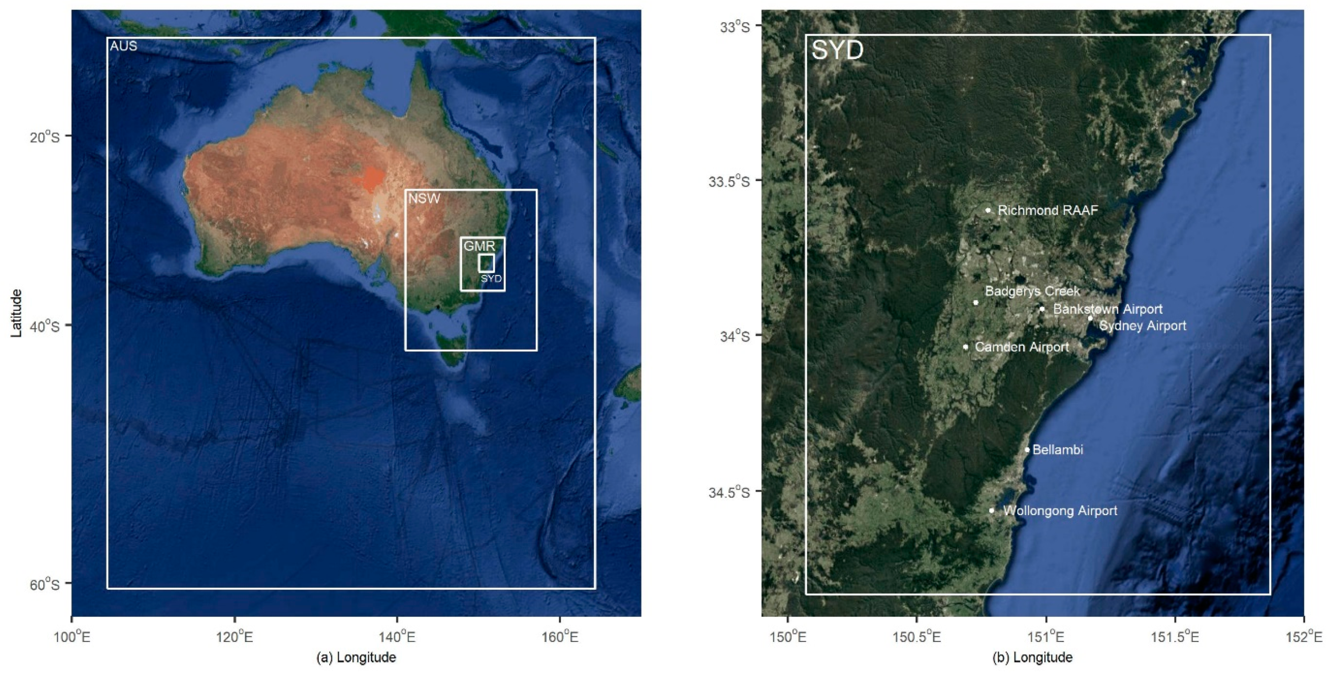
Figure 1. (a) Modelling domain configurations and the (b) location of Bureau of Meteorology Automatic Weather Stations used in this study. AUS: Australia NSW: New South Wales GMR: Greater Metropolitan Region SYD: Sydney domains.
Atmosphere 10 00374 g001
Figure 2. Near surface air temperature (°C) comparing observations and models grouped by each campaign (MUMBA, SPS1 and SPS2) for (a) mean diurnal cycle (observations are shown in black), (b) Taylor diagrams and (c) mean bias split by quantiles of observed values.
Atmosphere 10 00374 g002
Figure 3. Vertical profile of (a) mean bias (MB), (b) centred root mean square error (CRMSE) and (c) correlation coefficient (R) for temperature (°C) during each campaign (MUMBA, SPS1 and SPS2). The observations are from the twice daily radiosondes released at the BoM Sydney Airport site.
Atmosphere 10 00374 g003
Figure 4. Mixing ratio of water (g/kg) comparing observations and models grouped by each campaign (MUMBA, SPS1 and SPS2) for (a) mean diurnal cycle (observations are shown in black), (b) Taylor diagrams and (c) mean bias split by quantile bins.
Atmosphere 10 00374 g004
Figure 5. Vertical profile of (a) mean bias (MB), (b) centred root mean square error (CRMSE) and (c) correlation coefficient (R) for mixing ratio of water (g/kg) during each campaign (MUMBA, SPS1 and SPS2). The observations are from the twice daily radiosondes released at the BoM Sydney Airport site.
Atmosphere 10 00374 g005
Figure 6. Wind speed (m s−1) comparing observations and models grouped by each campaign (MUMBA, SPS1 and SPS2) for (a) mean diurnal cycle (observations are shown in black), (b) Taylor diagrams and (c) mean bias split by quantile bins.
Atmosphere 10 00374 g006
Figure 7. Quantile-quantile plots for wind speed (m s−1) comparing observations and models grouped by each campaign (MUMBA, SPS1 and SPS2).
Atmosphere 10 00374 g007
Figure 8. Vertical profile of (a) mean bias (MB), (b) centred root mean square error (CRMSE) and (c) correlation coefficient (R) for wind speed (m s−1) during each campaign (MUMBA, SPS1 and SPS2). The observations are from the twice daily radiosondes released at the BoM Sydney Airport site.
Atmosphere 10 00374 g008
Figure 9. Bubble plots of surface wind speed (m s−1) bias for all BoM weather stations for each model and campaign (MUMBA, SPS1 and SPS2).
Atmosphere 10 00374 g009
Figure 10. Zonal winds (m s−1) comparing observations and models grouped by each campaign (MUMBA, SPS1 and SPS2) for (a) mean diurnal cycle (observations are shown in black) and (b) Taylor diagrams.
Atmosphere 10 00374 g010
Figure 11. Averaged zonal wind (m s−1) profiles for (a) AM (morning) and (b) PM (afternoon) at the BoM Sydney Airport site for each campaign (MUMBA, SPS1 and SPS2).
Atmosphere 10 00374 g011
Figure 12. Planetary boundary layer height (PBLH—m) simulated (lines) and observed morning (AM—black dots) and afternoon (PM—black crosses in a box) for MUMBA, SPS1 and SPS2 campaign simulations.
Atmosphere 10 00374 g012
Figure 13. Taylor plots of PBLH (m) during the morning (AM) and afternoon (PM) for each campaign (MUMBA, SPS1 and SPS2).
Atmosphere 10 00374 g013
Figure 14. Time series of accumulated precipitation (mm) averaged over all BoM stations for each model and campaign (MUMBA, SPS1 and SPS2).
Atmosphere 10 00374 g014
Table 1. Overview of the configuration of the meteorological models.
Model IdentifierParameterW-UM1W-UM2W-A11O-CTMC-CTMW-NC1W-NC2
Research GroupUniv. MelbourneUniv. MelbourneANSTONSW OEHCSIRONCSUNCSU
Model specificationsMet. modelWRFWRFWRFCCAMCCAMWRFWRF
Chem. modelCMAQWRF-ChemWRF-Chem with simplified Radon onlyCSIRO-CTMCSIRO-CTMWRF-ChemWRF-Chem-ROMS
Met model version3.6.13.7.13.7.1r-4271:4285Mr-27963.7.13.7.1
DomainNx80, 73, 97, 10380, 73, 97, 10380, 73, 97, 10375, 60, 60, 6088,88,88,8879, 72, 96, 10279, 72, 96, 102
Ny70, 91, 97, 10370, 91, 97, 10370, 91, 97, 10365, 60, 60, 6088,88,88,8869, 90, 96, 10269, 90, 96, 102
Vertical layers33335035353232
Thickness of first layer (m)33.5561920203535
Initial & Boundary conditionsMet input/BCsERA InterimERA InterimERA InterimERA InterimERA InterimNCEP/FNLNCEP/FNL
Topography/Land useGeoscience Australia DEM for inner domain, USGS elsewhereGeoscience Australia DEM for inner domain. USGS elsewhere.Geoscience Australia DEM for inner domain, USGS elsewhere. MODIS land useMODISMODISUSGSUSGS
SSTHigh-res SST analysis (RTG_SST)High-res SST analysis (RTG_SST)High-res SST analysis (RTG_SST)SST from ERA InterimSSTs from ERA InterimHigh-res SST analysis (RTG_SST)Simulated by ROMS
Integration24-h simulations, each with 12-h spin-upContinuous with 2-d spin upContinuous with 10-d spin upContinuous with 1 mth spin up.Continuous with 1 mth spin up.Continuous with 8-d spin upContinuous with 8-d spin up
Data assimilationGrid-nudging outer domain above the PBLGrid-nudging outer domain above the PBLSpectral nudging in domain 1 above the PBL (scale-selective relaxation to analysis)Scale-selective filter to nudge towards the ERA-Interim dataScale-selective filter to nudge towards the ERA-Interim dataGridded analysis nudging above the PBLGridded analysis nudging above the PBL
ParameterisationsMicrophysicsMorrisonLinWSM6Prognostic condensate schemePrognostic condensate schemeMorrisonMorrison
LW radiationRRTMGRRTMGRRTMGGFDLGFDLRRTMGRRTMG
SW radiationRRTMGGSFCRRTMGGFDLGFDLRRTMGRRTMG
Land surfaceNOAHNOAHNOAHKowalczyk schemeKowalczyk schemeNOAHNOAH
PBLMYJYSUMYJLocal Richardson number and non-local stabilityLocal Richardson number and non-local stabilityYSUYSU
UCM3-category UCMNOAH UCMSingle layer UCMTown Energy budget approachTown Energy budget approachSingle layer UCMSingle layer UCM
ConvectionG3 (domains 1-3, off for domain 4)G3G3Mass-flux closureMass-flux closureMSKFMSKF
Aerosol feedbacksNoNoNoPrognostic aerosols with direct and indirect effectsPrognostic aerosols with direct and indirect effectsYesYes
Cloud feedbacksNoNoNoYesYesYesYes
ANSTO: Australian Nuclear Science and Technology Organisation WRF: Weather Research and Forecasting NSW OEH: New South Wales Office of Environment and Heritage CSIRO: Commonwealth Scientific and Industrial Research Organisation NCSU: North Carolina State University CCAM: Conformal Cubic Atmospheric Model BCs: Boundary Conditions ERA: European Centre for Medium Range Forecasting (ECMWF) Re-Analysis NCEP/FNL: National Centre for Environmental Prediction Final Analysis DEM: Digital Elevation Model USGS: United States Geological Survey MODIS: Moderate Resolution Imaging Spectroradiometer SST: Sea Surface Temperature PBL: Planetary Boundary Layer WSM6: WRF Single-Moment 6-class Scheme RRTMG: Rapid Radiative Transfer Model for GCMs GFDL: Geophysical Fluid Dynamics Scheme GSFC: Goddard Space Flight Centre Scheme MYJ: Mellor-Yamada-Janjic Scheme YSU: Yonsei University Scheme UCM: Urban Canopy Model G3: Grell 3D ensemble Scheme MSKF: Multi-Scale Kain-Fritsch Scheme.
Table 2. Measurement campaigns.
CampaignPeriod StartData Source
SPS107 February 2011–07 March 2011http://doi.org/10.4225/08/57903B83D6A5D
SPS216 April 2012–14 May 2012http://doi.org/10.4225/08/5791B5528BD63
MUMBA21 December 2012–15 February 2013http://doi.pangaea.de/10.1594/PANGAEA.871982
Table 3. Meteorological parameter benchmarks.
VariableStatistical MetricUnitsBenchmarkTerrain TypeSource
TemperatureMAE/Gross Errordegrees K≤2Simple[69]
≤3Complex[70]
Bias≤±0.5Simple[69]
≤±1Complex[70]
IOA-≥0.8 [69]
Mixing ratioMAE/Gross Errorg/kg≤2 [69]
Bias≤±1 [69]
IOA-≥0.6 [69]
Wind speedRMSEm s-1≤2Simple[69]
≤2.5Complex[70]
Bias≤±0.5Simple[69]
≤±1.5Complex[70]
IOA-≥0.6 [69]
Wind directionMAE/Gross ErrorDegrees≤30Simple[69]
≤55Complex[70]
Bias≤±10 [69]
Mean gross error (MAE), index of agreement (IOA).
Table 4. Normalised mean bias (%) of PBLH (m) for each model per campaign.
Time of DayStatisticModelCampaign
MUMBASPS1SPS2
AMNMB (%)C-CTM6626092
O-CTM−96147
W-A114118457
W-NC11912793
W-NC2813971
W-UM11587
W-UM217131167
Mean (m)Observations25513292
PMNMB (%)C-CTM17−29−1
O-CTM12−221
W-A1113−27−8
W-NC1−31−2611
W-NC2−22−18−10
W-UM1−1−31−13
W-UM2−36−26−11
Mean (m)Observations10481196985