Multiscale Applications of Two Online-Coupled Meteorology-Chemistry Models during Recent Field Campaigns in Australia, Part II: Comparison of WRF/Chem and WRF/Chem-ROMS and Impacts of Air-Sea Interactions and Boundary Conditions

Abstract

Air-sea interactions play an important role in atmospheric circulation and boundary layer conditions through changing convection processes and surface heat fluxes, particularly in coastal areas. These changes can affect the concentrations, distributions, and lifetimes of atmospheric pollutants. In this Part II paper, the performance of the Weather Research and Forecasting model with chemistry (WRF/Chem) and the coupled WRF/Chem with the Regional Ocean Model System (ROMS) (WRF/Chem-ROMS) are intercompared for their applications over quadruple-nested domains in Australia during the three following field campaigns: The Sydney Particle Study Stages 1 and 2 (SPS1 and SPS2) and the Measurements of Urban, Marine, and Biogenic Air (MUMBA). The results are used to evaluate the impact of air-sea interaction representation in WRF/Chem-ROMS on model predictions. At 3, 9, and 27 km resolutions, compared to WRF/Chem, the explicit air-sea interactions in WRF/Chem-ROMS lead to substantial improvements in simulated sea-surface temperature (SST), latent heat fluxes (LHF), and sensible heat fluxes (SHF) over the ocean, in terms of statistics and spatial distributions, during all three field campaigns. The use of finer grid resolutions (3 or 9 km) effectively reduces the biases in these variables during SPS1 and SPS2 by WRF/Chem-ROMS, whereas it further increases these biases for WRF/Chem during all field campaigns. The large differences in SST, LHF, and SHF between the two models lead to different radiative, cloud, meteorological, and chemical predictions. WRF/Chem-ROMS generally performs better in terms of statistics and temporal variations for temperature and relative humidity at 2 m, wind speed and direction at 10 m, and precipitation. The percentage differences in simulated surface concentrations between the two models are mostly in the range of ±10% for CO, OH, and O₃, ±25% for HCHO, ±30% for NO₂, ±35% for H₂O₂, ±50% for SO₂, ±60% for isoprene and terpenes, ±15% for PM_2.5, and ±12% for PM₁₀. WRF/Chem-ROMS at 3 km resolution slightly improves the statistical performance of many surface and column concentrations. WRF/Chem simulations with satellite-constrained boundary conditions (BCONs) improve the spatial distributions and magnitudes of column CO for all field campaigns and slightly improve those of the column NO₂ for SPS1 and SPS2, column HCHO for SPS1 and MUMBA, and column O₃ for SPS2 at 3 km over the Greater Sydney area. The satellite-constrained chemical BCONs reduce the model biases of surface CO, NO, and O₃ predictions at 3 km for all field campaigns, surface PM_2.5 predictions at 3 km for SPS1 and MUMBA, and surface PM₁₀ predictions at all grid resolutions for all field campaigns. A more important role of chemical BCONs in the Southern Hemisphere, compared to that in the Northern Hemisphere reported in this work, indicates a crucial need in developing more realistic chemical BCONs for O₃ in the relatively clean SH.

1. Introduction

Air-sea interactions have large impacts on atmospheric circulation and planetary boundary layer (PBL) conditions (such as the PBL height (PBLH), surface temperature, and surface wind) through changing coastal convection and surface fluxes exchange. The changes in PBL conditions will affect the concentrations, distributions, and lifetimes of atmospheric pollutants. While the impacts of air-sea interactions on atmospheric dynamics and ocean circulation have been assessed [1,2,3,4], their impacts on meteorology and atmospheric pollutants have not been extensively studied. He et al. [5] compared model simulations over the southern U.S. using the Weather Research and Forecasting model with Chemistry (WRF/Chem) without air-sea interactions, WRF/Chem with a 1-D ocean mixed layer model (WRF/Chem-OML), and WRF/Chem coupled with a 3-D Regional Ocean Modeling System (WRF/Chem-ROMS). They reported that the differences in the simulated surface concentrations of O₃ and PM_2.5 between WRF/Chem-ROMS and WRF/Chem can be as large as 17.3 ppb and 7.9 μg m⁻³, respectively, because WRF/Chem-ROMS explicitly simulates sea-surface temperature (SST), whereas WRF/Chem prescribes it. They also found that WRF/Chem-ROMS improves the predictions of most cloud and radiative variables and surface concentrations of a number of chemical species.

In addition to the model representations of major processes, the performance of a model is affected by the accuracy of the model inputs, such as emissions and initial and boundary conditions. The importance of chemical initial and boundary conditions (ICONs and BCONs) on air quality has been extensively studied in the Northern Hemisphere, but has seldom been reported for model applications in the Southern Hemisphere. These studies reported the impacts of ICONs and BCONs for several species including O₃ [6,7,8,9,10,11], CO [12], and particulate matter with diameters less than or equal to 2.5 and 10 μm (PM_2.5 and PM₁₀, respectively) [10,11,13,14], and their impacts on air quality. These studies suggested the use of spatial and time-varying BCONs, which can improve the model performance, compared to static or idealized BCONs [6,8,10,13]. They also reported sensitivity of the model predictions to chemical ICONs and BCONs derived from different global models. For example, Yahya et al. [11] compared 2006 and 2010 model predictions using WRF/Chem v3.4.1 with ICONs and BCONs from two global models, CESM and MACC, and found that the simulations with the CESM ICONs and BCONs improved the performance for O₃ mixing ratios in both years, PM_2.5 in 2010, and sulfate in 2006. Zhang et al. [12] showed substantial improvement for both spatial distribution and domain-mean performance statistics over the southeastern U.S. using satellite-constrained BCONs for O₃ and CO, reducing normalized mean biases (NMBs) of column O₃ and CO from 44.8% to −0.01% and −40.6% to −10.6%, respectively.

To understand the ambient air quality in Australia, in particular the Sydney area, evaluate the current models’ skill in reproducing atmospheric observations, and study the importance of air-sea interactions, the North Carolina State University’s version of WRF/Chem v3.7.1 (WRF/Chem-NCSU) and the coupled North Carolina State University’s WRF/Chem v3.7.1 with ROMS (WRF/Chem-ROMS) have been applied over quadruple-nested domains at grid resolutions of 81, 27, 9, and 3 km over Australia (d01), an area in southeastern Australia (d02), an area in New South Wales (d03), and in the Greater Sydney area (d04), respectively. The model simulations were performed during three field campaigns conducted in New South Wales (NSW), including the Sydney Particle Study (SPS) Stages 1 and 2 in western Sydney, during summer 2011 (5 February to 7 March) and autumn 2012 (16 April to 14 May), respectively [15,16], and the Measurements of Urban, Marine, and Biogenic Air (MUMBA) campaign in Wollongong during summer 2013 (21 December–15 February 2013) [17].

Part I presents a comprehensive evaluation of WRF/Chem-ROMS using surface data from the three field campaigns and satellite data. In this part II paper, the results from WRF/Chem are evaluated and compared with those of WRF/Chem-ROMS to assess the impact of air-sea interaction representation on meteorological and chemical predictions. In addition, the impact of chemical BCONs is assessed.

2. Model Description and Adjustment of Boundary Conditions

The two models used in this study are WRF/Chem-NCSU and WRF/Chem-ROMS. The model configurations and evaluation protocols are described in detail in the Part I paper. A more detailed description of WRF/Chem-NCSU can be found in Wang et al. [18] and Yahya et al. [19] and that of WRF/Chem-ROMS can be found in He et al. [5]. While WRF/Chem-NCSU is an online-coupled meteorology and chemistry model, WRF/Chem-ROMS is an online-coupled meteorology, chemistry, and ocean model. As indicated in Part I, the WRF/Chem-ROMS simulation uses the same physics and chemistry options as WRF/Chem with only one difference, WRF/Chem-ROMS explicitly represents air-sea interactions and simulates SST, whereas WRF/Chem-NCSU does not simulate air-sea interactions and it prescribes SST based on NCEP high-res SST analysis (RTG_SST) data [20,21]. The RTG_SST was generated based on satellite retrieval and created daily in near-real time (https://polar.ncep.noaa.gov/sst/rtg_high_res/description.shtml). This dataset has several weaknesses. For example, the resolution of data is relatively coarse with 0.5° × 0.5°, the accuracy of the data is directly affected by the satellite data used for the SST retrieval and, thus, contains relatively high uncertainties, compared to other reanalysis data, and the data may contain higher biases when the precipitating clouds are presented. Since the WRF/Chem simulation is initialized once at the beginning of the simulation, the prescribed SST remains constant throughout the simulation for each field campaign. For WRF/Chem-ROMS, the SST is simulated real-time and updated hourly.

In the initial applications of the two models, BCONs of CO, NO₂, HCHO, O₃, and PM_2.5 are calculated based on global model predictions from the Community Earth System Model (CESM-NCSU) v1.2.2. To improve the accuracy in the chemical boundary conditions, these values are adjusted using satellite-constrained values, which directly affect predictions over d01 at 81 km and indirectly affect predictions over the other domains (d02–d04). The satellite retrievals used for adjustment are the column abundance of carbon monoxide (CO) from the Measurements of Pollution in the Troposphere (MOPITT), columns of nitrogen dioxide (NO₂) and formaldehyde (HCHO) from the Global Ozone Monitoring Experiment (GOME), the tropospheric ozone residual (TOR) from the Ozone Monitoring Experiment (OMI), and the aerosol optical depth (AOD) (a proxy for aerosol column concentrations) from the Moderate Resolution Imaging Spectroradiometer (MODIS). The monthly average values from both satellite retrievals and CESM-NCSU, their ratios, as well as the average values along each side of the domain (by averaging a band containing 5 row or column of satellite retrievals depending on different side of boundaries) are first calculated. The four adjustment factors for each side are then calculated using these retrieval-to-model ratios and applied for all vertical profiles of the BCONs for these species. The adjustment factors for PM_2.5 are applied for the BCONs of all the major PM species. No adjustment is made for boundaries with poor quality of satellite data. Table S1 in the supplementary material summarizes the adjustment factors used for model simulations of SPS1, SPS2, and MUMBA. Using satellite retrievals as constraints, the values of BCONs are increased for CO, O₃, and HCHO and decreased for NO₂ for all three field campaign periods. Those for PM_2.5 are increased for SPS2 and MUMBA, but decreased for SPS2.

3. Impact of Explicit Representations of Air-Sea Interactions

3.1. Sea Surface Temperature and Surface Fluxes

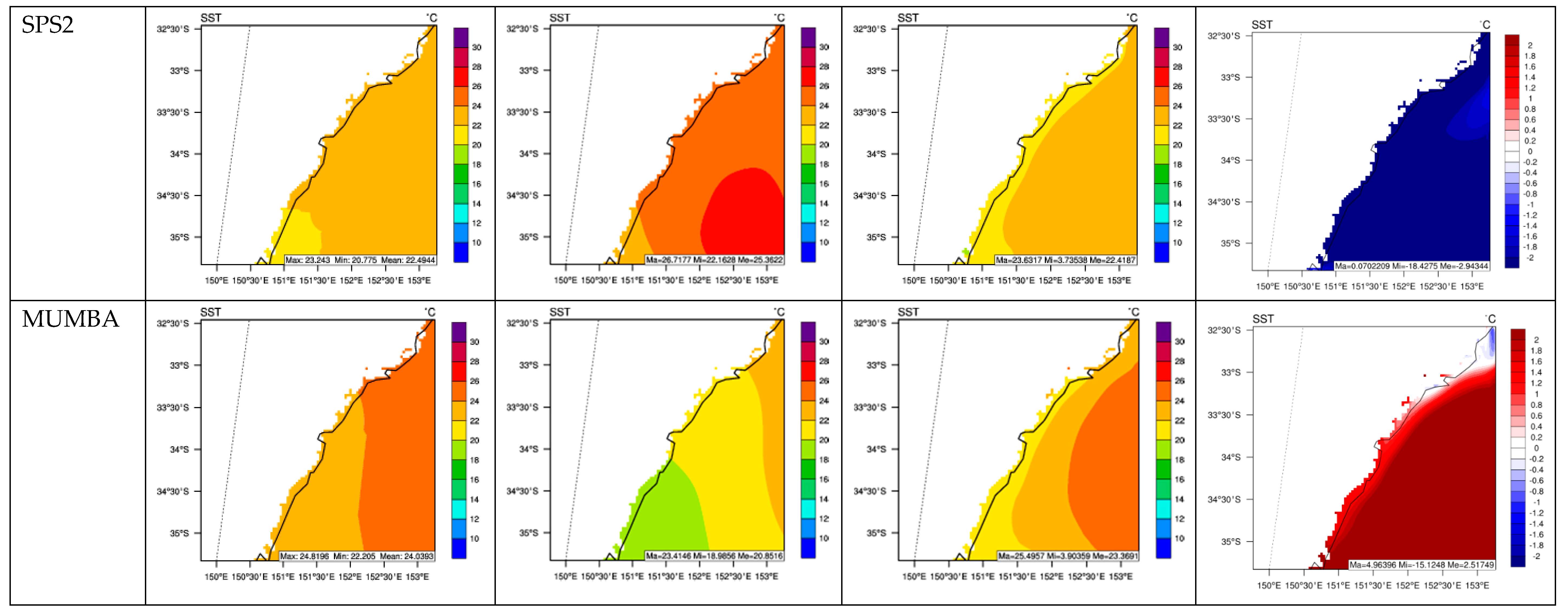
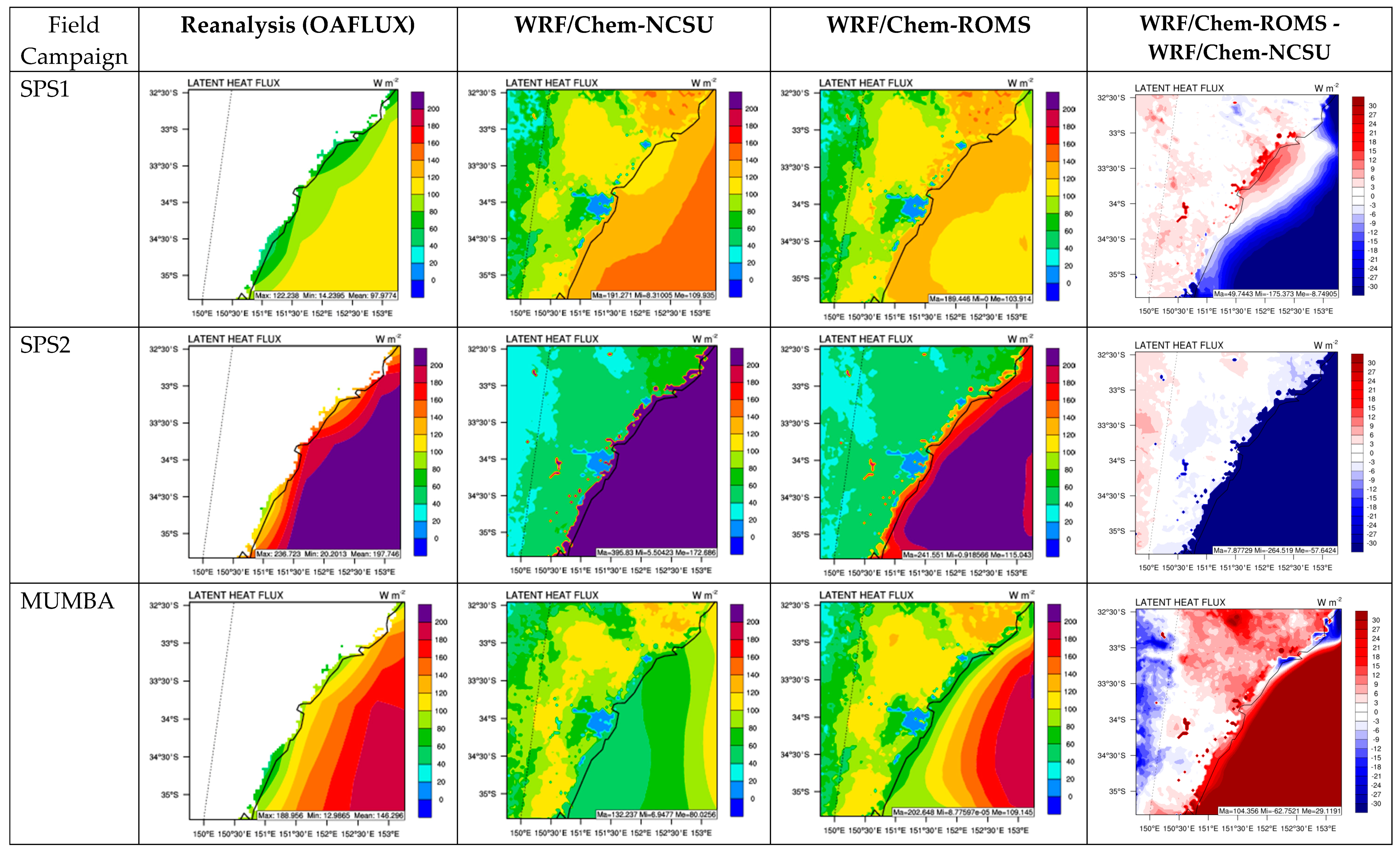
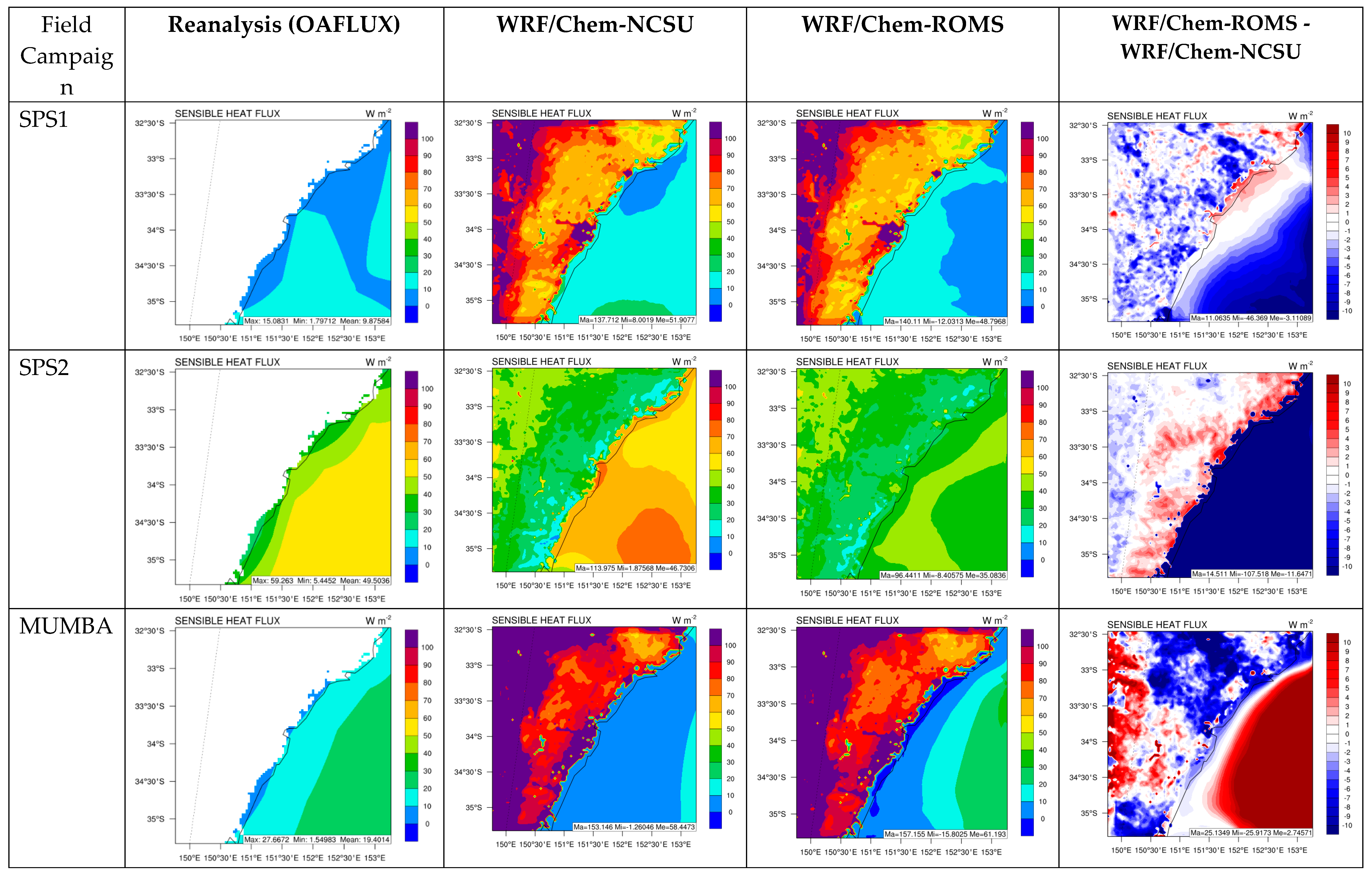
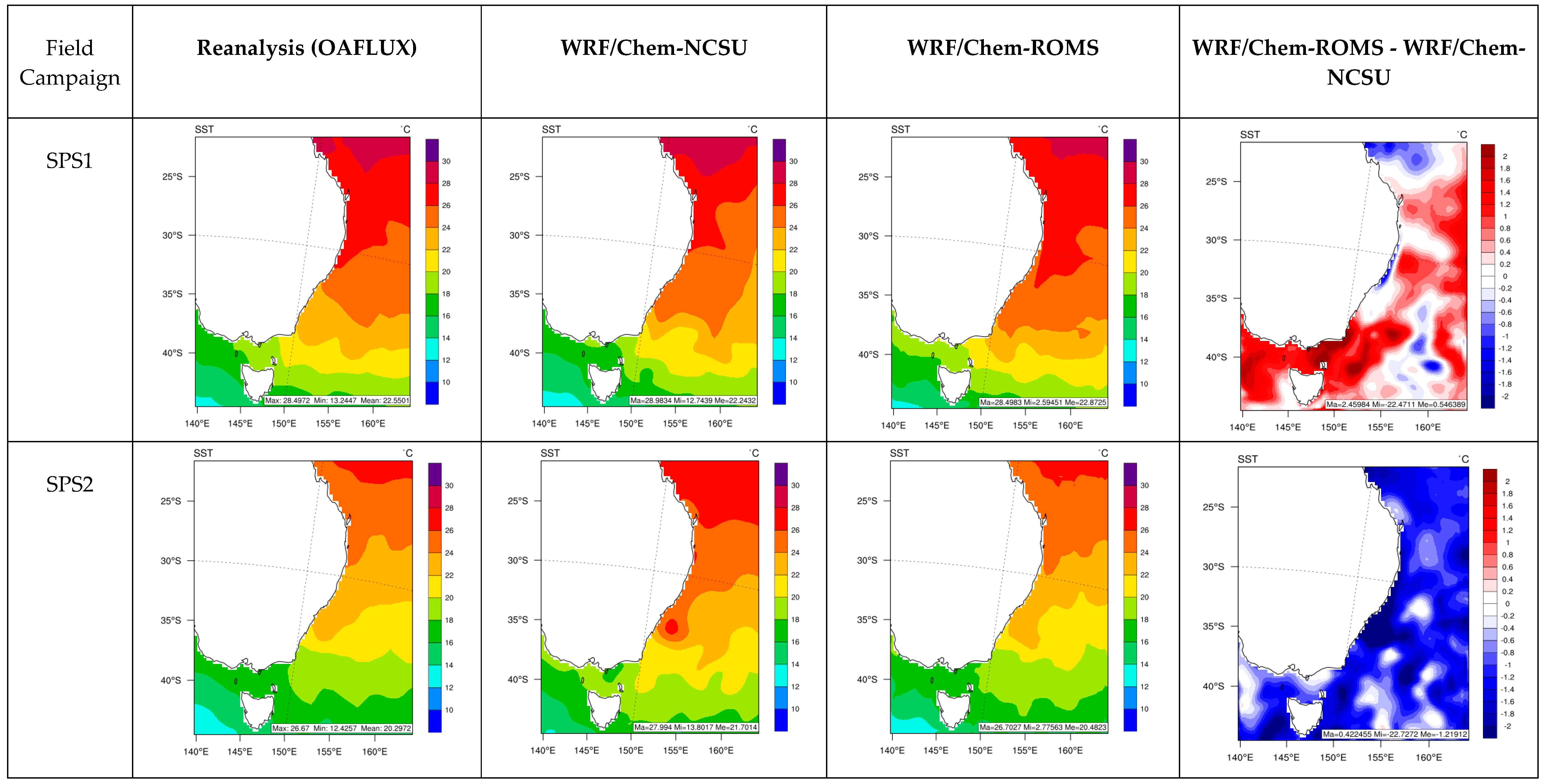
Air-sea interactions affect the marine boundary layer through the exchange of heat and momentum fluxes, which further affects large scale circulation, cloud formation, and precipitation, all of which in turn affect chemical concentrations of air pollutants. Unlike WRF/Chem-ROMS, that explicitly simulates air-sea interactions, WRF/Chem does not simulate air-sea interactions, instead, it uses prescribed SST from NCEP high-res SST analysis (RTG_SST) analysis data. To evaluate the impacts of explicit representation of air-sea interactions through the coupling of WRF/Chem and ROMS, simulated SST, latent heat flux (LHF), and sensible heat flux (SHF) from WRF/Chem-ROMS and prescribed SST and simulated LHF and SHF from WRF/Chem are evaluated using the Objectively Analyzed Air-Sea Fluxes (OAFlux) data [22].

Table 1. Mean bias (MB) and normalized mean bias (NMB) of meteorological and chemical variables from WRF/Chem and WRF/Chem-ROMS simulations at 81 km (d01), 27 km (d02), 9 km (d03), and 3 km (d04) over the 3 km domain (d04) for the SPS1 field campaign.

	WRF/Chem-ROMS								WRF/Chem
Variables	MB				NMB, %				MB				NMB, %
	d01	d02	d03	d04	d01	d02	d03	d04	d01	d02	d03	d04	d01	d02	d03	d04
Met
T2 (°C)	−0.9	−0.22	0.02	0.09	−4.1	−1.0	0.1	0.4	−1.11	−0.27	0.08	0.06	−5.0	−1.2	0.4	0.3
SST (°C)	1.4	1.0	0.5	0.6	5.9	4.2	2.3	2.9	0.9	0.9	0.9	0.9	3.9	4.0	4.0	3.9
RH2 (%)	−0.53	−1.95	−1.71	−0.7	−0.7	−2.8	−2.4	−1.0	0.40	−1.51	−1.55	−0.29	0.6	−2.1	−2.2	−0.5
WS10 (m s−1)	−0.56	−0.80	−0.35	−0.09	−15.3	−21.7	−9.7	−2.4	−0.52	−0.80	−0.3	−0.05	−14.3	−21.9	−8.2	−1.4
WD10 (°)	2.40	9.53	11.3	9.5	1.6	6.3	7.5	6.3	2.9	8.8	11.3	9.7	1.9	5.8	7.5	6.4
Precip (OBS) (mm day−1)	0.12	−0.01	−0.18	0.03	14.1	−0.7	−21.5	3.5	0.13	0.09	−0.06	0.07	15.7	10.5	−7.6	8.3
Precip. (MSWEP) (mm day−1)	−0.31	−0.36	−0.45	−0.16	−26.4	−30.5	−38.2	−13.4	−0.30	−0.28	−0.36	−0.17	−25.1	−23.5	−30.1	−14.8
Precip (GPCP) (mm day−1)	−1.3	−1.3	−1.5	−1.4	−59.1	−56.4	−69.6	−62.2	−1.3	−1.2	−1.5	−1.4	−59.7	−53.5	−68.4	−61.2
Chem
O3 (ppb)	2.96	0.09	−1.14	−0.97	17.4	0.5	−6.7	−5.7	2.80	−0.01	−0.99	−0.96	16.4	−0.1	−5.8	−5.7
CO (ppb)	−209.4	−166.9	−182.7	−146.4	−63.3	−46.6	−55.3	−44.3	−210.4	−169.5	−186.2	−147.1	−63.6	−51.3	−56.3	−44.5
NO (ppb)	−4.11	−1.56	−0.28	0.26	−84.5	−32.0	−5.8	5.0	−4.08	−1.57	−0.53	0.32	−83.9	−32.4	−10.8	6.5
NO2 (ppb)	−2.05	0.04	0.34	0.61	−32.3	0.7	5.4	9.6	−2.08	−0.09	0.16	0.59	−32.8	−1.4	2.5	9.3
SO2 (ppb)	0.31	0.62	0.58	0.70	50.7	100.9	94.9	114.3	0.28	0.57	0.54	0.67	46.0	93.5	87.9	110.2
PM2.5 (μgm−3)	−2.30	−1.66	−1.51	−1.36	−40.2	−29.1	−26.5	−23.7	−2.34	−1.71	−1.62	−1.44	−41.0	−29.9	−28.4	−25.2
PM10 (μgm−3)	−10.6	−9.9	−9.8	−9.4	−59.4	−55.6	−55.4	−52.9	−10.6	−9.9	−9.9	−9.6	−59.8	−55.6	−55.9	−53.8

Mean Obs and Sim: Time average across all grids with observations in each domain based on either hourly or daily predictions and observations, respectively; R: correlation coefficient; MB: mean bias; NMB: normalized mean bias; NME: normalized mean error; T2: 2 m temperature; SST: sea surface temperature; RH2: 2 m relative humidity; WS10: 10 m wind speed; WD10: 10 m wind direction; Precip: precipitation; O₃: ozone; CO: carbon monoxide; NO: nitric oxide; NO₂: nitrogen dioxide; SO₂: sulfur dioxide; PM_2.5 and PM₁₀: particulate matter with aerodynamic diameters ≤2.5 μm and 10 μm; OBS: the observations based on the Bureau of Meteorology (BoM) measurements; MSWEP: the Multi-Source Weighted-Ensemble Precipitation; and GPCP: the Global Precipitation Climatology Project. All observational data are based on the BoM measurements unless otherwise noted. Precipitation is evaluated against the three following datasets: OBS, MSWEP, and GPCP.

,

Table 2. Mean bias (MB) and normalized mean bias (NMB) of meteorological and chemical variables from WRF/Chem and WRF/Chem-ROMS simulations at 81 km (d01), 27 km (d02), 9 km (d03), and 3 km (d04) over the 3 km domain (d04) for the SPS2 field campaign.

	WRF/Chem-ROMS								WRF/Chem
Variables	MB				NMB, %				MB				NMB, %
	d01	d02	d03	d04	d01	d02	d03	d04	d01	d02	d03	d04	d01	d02	d03	d04
Met
T2 (°C)	−0.7	−0.1	−0.2	0.1	−4.6	0.6	−1.0	0.4	−0.07	0.36	0.14	0.37	−0.4	2.3	0.9	2.4
SST (°C)	−1.7	−0.5	−0.4	−0.1	−7.5	−2.2	−1.9	−0.4	1.8	2.4	2.6	2.9	7.9	10.8	11.7	12.7
RH2 (%)	0.5	−4.4	−4.1	−5.2	0.6	−5.9	−5.5	−6.9	−3.0	−6.6	−7.0	−8.1	−4.0	−8.8	−9.3	−10.7
WS10 (m s−1)	1.00	0.63	0.12	0.16	37.6	23.7	4.4	6.1	1.15	0.74	0.20	0.25	43.3	28.0	7.4	9.5
WD10 (°)	−1.6	2.6	4.2	1.9	−0.8	1.4	2.2	1.0	−3.4	2.7	3.8	2.8	−1.8	1.4	2.0	1.5
Precip (OBS) (mm day−1)	−1.16	−0.53	−1.33	−1.38	−26.3	−12.1	−30.2	−31.3	−0.76	−1.45	−1.94	−2.06	−17.1	−32.9	−44.0	−46.7
Precip. (MSWEP) (mm day−1)	−1.29	−0.67	−1.47	−1.52	−28.5	−14.8	−32.3	−33.4	−0.89	−1.59	−2.08	−2.20	−19.6	−35.0	−45.7	−48.3
Precip (GPCP) (mm day−1)	0.2	0.5	0.0	−0.1	10.6	23.5	0.3	−6.6	1.5	1.6	0.6	0.5	63.3	70.0	27.7	21.3
Chem
O3 (ppb)	2.65	−0.02	−1.26	−0.44	20.5	−0.2	−9.8	−3.4	3.96	0.91	−0.25	0.64	30.7	7.0	−1.9	4.9
CO (ppb)	−223.7	−121.6	−116.1	−92.9	−58.9	−32.0	−30.6	−24.5	−223.7	−128.9	−133.7	−114.6	−58.9	−34.0	−35.2	−30.2
NO (ppb)	−11.3	−5.63	0.59	1.65	−89.3	−44.6	4.7	13.0	−11.6	−6.56	−0.9	−0.01	−91.8	−51.9	−7.1	−0.1
NO2 (ppb)	−2.71	0.48	1.84	2.2	−29.5	5.3	20.1	24.0	−3.01	−0.00	1.38	1.67	−32.8	−0.0	15.1	18.2
SO2 (ppb)	0.39	0.82	0.86	0.98	63.3	134.8	141.0	160.5	0.44	0.78	0.75	0.87	71.3	126.8	123.3	141.4
PM2.5 (μgm−3)	−0.18	2.73	6.3	8.0	−3.4	49.7	114.8	145.6	−0.27	2.25	5.75	7.57	−5.0	41.0	104.6	137.9
PM10 (μgm−3)	−5.0	−3.1	−1.33	−0.28	−34.9	−21.8	−9.3	−1.9	−4.8	−4.0	−2.08	−1.0	−33.5	−28.3	−14.5	−7.0

Mean Obs and Sim: Time average across all grids with observations in each domain based on either hourly or daily predictions and observations, respectively; R: correlation coefficient; MB: mean bias; NMB: normalized mean bias; NME: normalized mean error; T2: 2 m temperature; SST: sea surface temperature; RH2: 2 m relative humidity; WS10: 10 m wind speed; WD10: 10 m wind direction; Precip: precipitation; O₃: ozone; CO: carbon monoxide; NO: nitric oxide; NO₂: nitrogen dioxide; SO₂: sulfur dioxide; PM_2.5 and PM₁₀: particulate matter with aerodynamic diameters ≤2.5 μm and 10 μm; OBS: the observations based on the Bureau of Meteorology (BoM) measurements; MSWEP: the Multi-Source Weighted-Ensemble Precipitation; GPCP: the Global Precipitation Climatology Project. All observational data are based on the BoM measurements unless otherwise noted. Precipitation is evaluated against the three following datasets: OBS, MSWEP, and GPCP.

and

Table 3. Mean bias (MB) and normalized mean bias (NMB) of meteorological and chemical variables from WRF/Chem and WRF/Chem-ROMS simulations at 81 km (d01), 27 km (d02), 9 km (d03), and 3 km (d04) over the 3 km domain (d04) for the MUMBA field campaign.

	WRF/Chem-ROMS								WRF/Chem
Variables	MB				NMB, %				MB				NMB, %
	d01	d02	d03	d04	d01	d02	d03	d04	d01	d02	d03	d04	d01	d02	d03	d04
Met
T2 (°C)	−0.5	0.1	−0.05	−0.2	−2.2	0.4	−0.2	−0.9	−1.9	−1.3	−1.0	−1.1	−8.6	−5.6	−4.6	−4.9
SST (°C)	0.4	0.3	−0.3	−0.5	1.8	1.3	−1.3	−2.1	−2.9	−3.1	−3.2	−3.3	−12.2	−13.0	−13.3	−13.6
RH2 (%)	0.4	−1.0	−0.6	−0.4	0.6	−1.5	−0.8	−0.5	4.5	2.8	2.4	2.5	6.3	4.0	3.4	3.5
WS10 (m s−1)	0.16	−0.21	−0.29	−0.32	4.3	−5.4	−7.5	−8.4	−0.04	−0.28	−0.33	−0.37	−1.0	−7.3	−8.6	−9.6
WD10 (°)	3.4	10.8	11.5	10.9	2.4	7.8	8.3	7.8	4.9	10.5	10.9	10.6	3.5	7.6	7.9	7.7
Precip (OBS) (mm day−1)	−1.65	−1.82	−1.67	−2.06	−32.4	−35.9	−32.9	−40.7	−2.11	−1.78	−2.09	−1.89	−41.6	−35.1	−41.1	−37.2
Precip. (MSWEP) (mm day−1)	−1.55	−1.73	−1.58	−1.97	−31.3	−34.7	−31.7	−39.5	−2.02	−1.69	−1.99	−1.79	−40.5	−33.9	−40.0	−36.0
Precip (GPCP) (mm day−1)	−2.3	−2.0	−2.3	−2.8	−42.2	−36.8	−41.9	−50.7	−3.1	−2.6	−2.7	−3.2	−57.1	−47.6	−48.9	−56.9
Chem
O3 (ppb)	2.96	0.52	−1.26	−1.84	16.2	2.8	−6.9	−10.1	1.6	−1.0	−2.3	−2.84	8.5	−5.6	−12.4	−15.6
CO (ppb)	−136.9	−102.8	−109.6	−63.7	−54.9	−41.2	−43.9	−25.5	−130.2	−96.6	−102.6	−45.4	−52.2	−38.7	−41.1	−18.2
NO (ppb)	−2.06	−0.48	0.49	1.41	−77.3	−18.1	18.3	53.2	−1.83	0.05	0.84	2.31	−68.9	2.0	31.4	86.9
NO2 (ppb)	−1.44	0.29	0.90	1.46	−30.2	6.2	18.8	30.7	−1.12	0.78	1.19	1.84	−23.6	16.4	25.0	38.7
SO2 (ppb)	0.21	0.51	0.61	0.92	33.8	83.5	98.8	149.6	0.23	0.49	0.61	0.90	37.4	80.5	99.4	146.6
PM2.5 (μgm−3)	−4.2	−3.65	−3.51	−3.27	−56.4	−48.6	−46.7	−43.6	−4.4	−3.8	−3.6	−3.42	−58.6	−51.0	−48.5	−45.6
PM10 (μgm−3)	−12.2	−11.5	−11.6	−10.9	−59.4	−56.3	−56.4	−53.4	−13.0	−12.2	−12.0	−11.2	−63.7	−59.6	−58.5	−54.7

Mean Obs and Sim: Time average across all grids with observations in each domain based on either hourly or daily predictions and observations, respectively; R: correlation coefficient; MB: mean bias; NMB: normalized mean bias; NME: normalized mean error; T2: 2 m temperature; SST: sea surface temperature; RH2: 2 m relative humidity; WS10: 10 m wind speed; WD10: 10 m wind direction; Precip: precipitation; O₃: ozone; CO: carbon monoxide; NO: nitric oxide; NO₂: nitrogen dioxide; SO₂: sulfur dioxide; PM_2.5 and PM₁₀: particulate matter with aerodynamic diameters ≤ 2.5 μm and 10 μm; OBS: the observations based on the Bureau of Meteorology (BoM) measurements; MSWEP: the Multi-Source Weighted-Ensemble Precipitation; GPCP: the Global Precipitation Climatology Project. All observational data are based on the BoM measurements unless otherwise noted. Precipitation is evaluated against the following three datasets: OBS, MSWEP, and GPCP.

compare the performance statistics in terms of mean bias (MB) and normalized mean bias (NMB) for SST and

Table 4. Mean bias (MB) and normalized mean bias (NMB) of column variables from WRF/Chem and WRF/Chem-ROMS simulations at 81 km (d01), 27 km (d02), 9 km (d03), and 3 km (d04) over the 3 km domain (d04) for the SPS1 field campaign.

Satellite Variables	Network	WRF/Chem-ROMS								WRF/Chem
		MB				NMB, %				MB				NMB, %
		d01	d02	d03	d04	d01	d02	d03	d04	d01	d02	d03	d04	d01	d02	d03	d04
LHF (W m−2)	OAFlux	47.5	36.8	22.5	25.2	49.4	38.2	23.4	26.2	40.8	42.0	39.5	38.3	42.4	43.7	41.1	39.8
SHF (W m−2)	OAFlux	7.1	4.3	2.6	1.5	74.2	45.2	27.3	16.0	8.7	7.5	7.0	5.4	90.8	77.6	73.1	56.4
GLW (W m−2)	CERES	−15.5	−15.1	−15.8	−17.2	−3.9	−3.8	−4.0	−4.4	−15.3	−13.9	−13.9	−15.8	−3.9	−3.5	−3.5	−4.0
GSW (W m−2)	CERES	50.0	46.9	50.0	56.6	24.5	23.0	24.5	27.8	47.1	44.4	47.0	54.1	23.1	21.8	23.1	26.6
LWCF (W m−2)	CERES	−16.4	−14.8	−15.6	−20.4	−44.4	−40.0	−42.2	−55.1	−16.5	−14.7	−15.4	−20.3	−44.6	−39.7	−41.8	−54.9
SWCF (W m−2)	CERES	−45.0	−40.3	−44.0	−51.0	−53.4	−47.8	−52.1	−60.4	−42.8	−38.1	−41.5	−48.9	−50.7	−45.1	−49.1	−57.9
AOD	MODIS	0.0	0.01	0.01	0.01	1.6	6.4	8.3	7.3	0.0	0.01	0.01	0.01	3.1	7.2	9.2	7.9
COT	MODIS	−11.1	−9.7	−11.8	−12.6	−70.4	−62.0	−74.9	−80.4	−9.7	−9.5	−11.5	−12.4	−61.7	−60.6	−73.4	−79.1
CCN	MODIS	−0.0	−0.0	−0.0	−0.0	−22.7	−19.4	−17.4	−12.7	−0.0	−0.0	−0.0	−0.0	−23.1	−17.9	−16.8	−12.8
CDNC (# m−3)	MODIS	−51.2	4.6	−6.9	−32.6	−46.2	3.5	−6.2	−31.2	−44.2	−17.4	−35.3	−40.2	−40.0	−15.7	−32.1	−37.3
CF	MODIS	−0.3	−0.2	−0.2	−0.3	−46.3	−39.4	−40.9	−45.6	−0.3	−0.2	−0.2	−0.3	−43.1	−36.2	−38.6	−43.4
LWP	MODIS	−119.4	−115.6	−113.2	−109.9	−96.8	−93.7	−91.7	−89.1	−117.9	−114.6	−111.6	−108.5	−95.5	−92.9	−90.5	−88.0
PWV	MODIS	−0.5	−0.4	−0.4	−0.4	−12.1	−11.6	−11.7	−11.7	−0.5	−0.4	−0.4	−0.4	−12.1	−11.4	−11.4	−11.4
Column CO (1018 molecules cm−2)	MOPITT	−0.3	−0.3	−0.3	−0.3	−22.0	−21.8	−21.6	−21.4	−0.3	−0.3	−0.3	−0.3	−22.0	−21.7	−21.6	−21.3
Column NO2 (1015 molecules cm−2)	GOME	−1.0	−0.7	−0.5	−0.5	−43.1	−30.9	−23.6	−22.7	−0.9	−0.7	−0.5	−0.5	−42.6	−31.2	−24.8	−23.2
Column HCHO (1015 molecules cm−2)	GOME	−1.2	−1.5	−1.6	−1.6	−16.4	−20.5	−22.6	−21.7	−1.2	−1.5	−1.6	−1.6	−17.0	−20.8	−22.8	−21.9
TOR (DU)	OMI	6.6	6.2	5.9	5.7	26.9	25.2	23.9	23.1	6.6	6.2	5.8	5.7	26.9	25.1	23.8	23.0

Mean Obs and Sim: Time average across all grids with observations in each domain based on either hourly or daily predictions and observations, respectively; R: correlation coefficient; MB: mean bias; NMB: normalized mean bias; NME: normalized mean error; LHF: latent heat flux; SHF: sensible heat flux; GLW; downward longwave radiation; GSW: net shortwave radiation; LWCF: longwave cloud forcing; SWCF: shortwave cloud forcing; AOD: aerosol optical depth; COT: cloud optical thickness; CCN: cloud condensation nuclei; CDNC: cloud droplet number concentration: CF: cloud fraction; LWP: cloud liquid water path; PWV: precipitating water vapor; CO: carbon monoxide; NO₂: nitrogen dioxide; HCHO: formaldehyde; TOR: tropospheric ozone residual; DU: Dobson Unit; OAFlux: the Objectively Analyzed Air-Sea Fluxes; CERES: the Clouds and the Earth’s Radiant Energy System; MODIS: the Moderate Resolution Imaging Spectroradiometer; MOPITT: Measurements of Pollution in the Troposphere; GOME: the Global Ozone Monitoring Experiment; OMI: the Ozone Monitoring Experiment.

,

Table 5. Mean bias (MB) and normalized mean bias (NMB) of column variables from WRF/Chem and WRF/Chem-ROMS simulations at 81 km (d01), 27 km (d02), 9 km (d03), and 3 km (d04) over the 3 km domain for the SPS2 field campaign.

Satellite Variables	Network	WRF/Chem-ROMS								WRF/Chem
		MB				NMB, %				MB				NMB, %
		d01	d02	d03	d04	d01	d02	d03	d04	d01	d02	d03	d04	d01	d02	d03	d04
LHF (W m−2)	OAFlux	−39.1	−4.9	−5.5	3.6	−19.9	−2.4	−2.7	1.8	105.1	121.9	127.3	131.8	53.4	62.0	64.8	67.0
SHF (W m−2)	OAFlux	−22.3	−14.7	−12.9	−11.3	−45.3	−29.9	−26.2	−22.9	6.1	12.5	15.3	15.7	12.5	25.4	31.0	31.8
GLW (W m−2)	CERES	−7.3	−6.4	−7.3	−9.1	−2.2	−1.9	−2.2	−2.7	−2.4	−3.1	−4.8	−7.4	−0.7	−0.9	−1.4	−2.2
GSW (W m−2)	CERES	6.7	8.1	10.9	16.3	5.2	6.2	8.5	12.7	3.8	5.5	10.1	16.4	2.9	4.3	7.8	12.8
LWCF (W m−2)	CERES	−4.6	−2.3	−3.7	−8.3	−19.0	−9.8	−15.2	−34.5	−1.6	−0.3	−2.6	−7.5	−6.7	−1.4	−10.6	−31.1
SWCF (W m−2)	CERES	−1.9	−1.4	−4.6	−10.6	−5.6	−4.1	−13.4	−31.1	1.0	0.9	−3.6	−10.4	2.7	2.5	−10.4	−30.5
AOD	MODIS	0.06	0.06	0.06	0.06	73.6	76.6	73.4	71.0	0.06	0.06	0.06	0.04	73.9	76.7	70.5	66.4
COT	MODIS	−2.7	−2.7	−6.4	−8.8	−18.7	−19.0	−44.5	−61.2	1.5	0.3	−4.8	−7.9	10.6	2.0	−33.2	−55.1
CCN	MODIS	−0.1	−0.1	−0.1	−0.0	−28.2	−27.8	−27.5	−24.1	−0.1	−0.1	−0.1	−0.0	−27.5	−28.5	−26.1	−22.9
CDNC (# m−3)	MODIS	-	-	-	-	-	-	-	-	-	-	-	-	-	-	-	-
CF	MODIS	−0.1	−0.1	−0.1	−0.2	−26.4	−26.8	−25.9	−32.2	−0.1	−0.1	−0.1	−0.2	−26.1	−24.4	−25.9	−34.9
LWP	MODIS	−136.0	−135.6	−134.8	−133.9	−95.1	−94.7	−94.2	−93.6	−134.7	−130.9	−130.2	−131.2	−94.1	−91.5	−91.0	−91.6
PWV	MODIS	0.3	0.3	0.3	0.3	21.1	21.3	21.0	21.0	0.3	0.3	0.3	0.3	23.1	22.7	22.3	21.9
Column CO (1018 molecules cm−2)	MOPITT	−0.1	−0.1	−0.1	−0.1	−7.3	−7.1	−7.0	−6.8	−0.1	−0.1	−0.1	−0.1	−7.3	−7.0	−7.0	−6.8
Column NO2 (1015 molecules cm−2)	GOME	−1.0	−0.7	−0.6	−0.5	−35.2	−25.4	−21.5	−19.4	−1.0	−0.7	−0.6	−0.6	−37.6	−26.3	−23.2	−21.2
Column HCHO (1015 molecules cm−2)	GOME	−0.9	−1.0	−1.0	−0.9	−25.0	−26.6	−27.4	−25.6	−0.8	−0.9	−0.9	−0.9	−23.1	−25.4	−25.8	−24.1
TOR (DU)	OMI	1.5	1.5	1.3	1.3	5.2	5.0	4.4	4.3	1.7	1.6	1.5	1.5	5.9	5.6	5.1	5.1

Mean Obs and Sim: Time average across all grids with observations in each domain based on either hourly or daily predictions and observations, respectively; R: correlation coefficient; MB: mean bias; NMB: normalized mean bias; NME: normalized mean error; LHF: latent heat flux; SHF: sensible heat flux; GLW; downward longwave radiation; GSW: net shortwave radiation; LWCF: longwave cloud forcing; SWCF: shortwave cloud forcing; AOD: aerosol optical depth; COT: cloud optical thickness; CCN: cloud condensation nuclei; CDNC: cloud droplet number concentration: CF: cloud fraction; LWP: cloud liquid water path; PWV: precipitating water vapor; CO: carbon monoxide; NO₂: nitrogen dioxide; HCHO: formaldehyde; TOR: tropospheric ozone residual; DU: Dobson Unit; OAFlux: the Objectively Analyzed Air-Sea Fluxes; CERES: the Clouds and the Earth’s Radiant Energy System; MODIS: the Moderate Resolution Imaging Spectroradiometer; MOPITT: Measurements of Pollution in the Troposphere; GOME: the Global Ozone Monitoring Experiment; OMI: the Ozone Monitoring Experiment.

and

Table 6. Mean bias (MB) and normalized mean bias (NMB) (%) of column variables from WRF/Chem and WRF/Chem-ROMS simulations at 81 km (d01), 27 km (d02), 9 km (d03), and 3 km (d04) over the 3 km domain for the MUMBA field campaign.

Satellite Variables	Network	WRF/Chem-ROMS								WRF/Chem
		MB				NMB, %				MB				NMB, %
		d01	d02	d03	d04	d01	d02	d03	d04	d01	d02	d03	d04	d01	d02	d03	d04
LHF (W m−2)	OAFlux	11.8	7.7	−9.8	−14.2	8.1	5.3	−6.8	−9.9	−73.8	−76.4	−79.0	−81.4	−51.4	−53.2	−55.0	−56.7
SHF (W m−2)	OAFlux	1.4	−1.6	−3.6	−6.7	7.3	−8.4	−19.0	−35.5	−7.9	−10.6	−12.1	−15.1	−42.1	−56.0	−63.8	−79.9
GLW (W m−2)	CERES	−15.0	−13.0	−14.1	−15.7	−3.9	−3.4	−3.7	−4.1	−18.0	−15.3	−14.7	−16.5	−4.7	−4.0	−3.8	−4.3
GSW (W m−2)	CERES	51.6	49.2	51.6	57.3	22.8	21.7	22.8	25.3	50.8	47.6	48.5	53.8	22.4	21.0	21.4	23.8
LWCF (W m−2)	CERES	−18.7	−18.1	−19.2	−20.4	−63.0	−61.2	−64.6	−68.8	−19.6	−18.9	−19.5	−20.7	−66.1	−63.9	−65.9	−69.9
SWCF (W m−2)	CERES	−39.5	−35.2	−37.7	−43.3	−50.1	−44.7	−47.9	−55.0	−38.5	−33.4	−34.8	−40.2	−48.9	−42.4	−44.2	−51.0
AOD	MODIS	0.03	0.04	0.05	0.04	27.2	32.3	34.5	33.0	0.03	0.03	0.04	0.04	23.7	27.7	28.8	27.8
COT	MODIS	−6.4	−6.9	−10.2	−12.1	−37.4	−40.5	−59.7	−71.0	−10.5	−9.4	−11.3	−12.6	−61.6	−55.2	−66.1	−73.7
CCN	MODIS	−0.2	−0.2	−0.2	−0.2	−57.9	−56.7	−56.3	−54.4	−0.2	−0.2	−0.2	−0.2	−60.3	−59.6	−57.8	−55.4
CDNC (# m−3)	MODIS	-	-	-	-	-	-	-	-	-	-	-	-	-	-	-	-
CF	MODIS	−0.4	−0.3	−0.3	−0.3	−65.8	−56.9	−48.7	−55.5	−0.3	−0.3	−0.2	−0.3	−55.1	−43.6	−35.7	−43.3
LWP	MODIS	−143.8	−140.3	−136.4	−134.6	−97.1	−94.7	−92.1	−90.9	−141.4	−137.0	−134.3	−132.8	−95.5	−92.5	−90.7	−89.6
PWV	MODIS	0.4	0.4	0.4	0.4	17.7	18.6	18.2	18.3	0.4	0.4	0.4	0.4	16.3	17.1	17.1	17.3
Column CO (1018 molecules cm−2)	MOPITT	−0.2	−0.2	−0.2	−0.2	−17.4	−17.2	−17.2	−17.0	−0.2	−0.2	−0.2	−0.2	−17.5	−17.2	−17.2	−17.1
Column NO2 (1015 molecules cm−2)	GOME	−0.6	−0.4	−0.2	−0.2	−34.2	−21.6	−15.4	−11.5	−0.5	−0.3	−0.2	−0.2	−29.5	−20.1	−15.2	−12.4
Column HCHO (1015 molecules cm−2)	GOME	0.0	−0.3	−0.6	−0.5	−0.1	−7.1	−11.4	−10.0	−0.2	−0.5	−0.7	−0.6	−5.0	−9.6	−13.2	−11.8
TOR (DU)	OMI	13.9	13.5	13.3	13.1	42.0	40.6	40.1	39.4	13.8	13.4	13.2	12.9	41.8	40.4	39.9	39.0

Obs: Mean Obs and Sim: Time average across all grids with observations in each domain based on either hourly or daily predictions and observations, respectively; R: correlation coefficient; MB: mean bias; NMB: normalized mean bias; NME: normalized mean error; LHF: latent heat flux; SHF: sensible heat flux; GLW; downward longwave radiation; GSW: net shortwave radiation; LWCF: longwave cloud forcing; SWCF: shortwave cloud forcing; AOD: aerosol optical depth; COT: cloud optical thickness; CCN: cloud condensation nuclei; CDNC: cloud droplet number concentration: CF: cloud fraction; LWP: cloud liquid water path; PWV: precipitating water vapor; CO: carbon monoxide; NO₂: nitrogen dioxide; HCHO: formaldehyde; TOR: tropospheric ozone residual; DU: Dobson Unit; OAFlux: the Objectively Analyzed Air-Sea Fluxes; CERES: the Clouds and the Earth’s Radiant Energy System; MODIS: the Moderate Resolution Imaging Spectroradiometer; MOPITT: Measurements of Pollution in the Troposphere; GOME: the Global Ozone Monitoring Experiment; OMI: the Ozone Monitoring Experiment.

compare MBs and NMBs of LHF and SHF simulated by WRF/Chem-NCSU and WRF/Chem-ROMS over oceanic areas during SPS1, SPS2, and MUMBA, respectively. Figure 1 and Figure 2 compare prescribed SST based on the NCEP high-res SST analysis data by WRF/Chem-NCSU and simulated SST by WRF/Chem-ROMS at 27 and 3 km grid resolutions, respectively, with estimated SST from a combined satellite retrievals, modeling, and reanalysis dataset, OAFlux, over the Greater Sydney area (d04). Figure 3 and Figure S1 and Figure 4 and Figure S2 compare simulated LHF and SHF, respectively, by both models at 27 and 3 km grid resolution with OAFlux estimates over d04. For SPS1, mean biases (MBs) of SST are 0.9 °C from WRF/Chem at all grid resolutions but 1.4 °C, 1.0 °C, 0.5 °C, and 0.6 °C from WRF/Chem-ROMS at 81, 27, 9, and 3km, respectively. Although SST from both models is higher than SST from OAFlux, the use of finer grid resolutions (3 and 9km) reduces the mean biases in simulated SST by WRF/Chem-ROMS. For SPS2, MBs of SST are 1.8 °C, 2.4 °C, 2.6 °C, and 2.9 °C from WRF/Chem and −1.7 °C, −0.5 °C, −0.4 °C, and −0.1 °C from WRF/Chem-ROMS at 81, 27, 9, and 3 km, respectively. The use of finer grid resolutions reduces the biases to a much larger extent than SPS1 in simulated SST by WRF/Chem-ROMS, whereas it further increases the warm biases for WRF/Chem. While prescribed SST from WRF/Chem is much higher than SST from OAFlux over most of the oceanic area, that from WRF/Chem-ROMS shows a substantial improvement over most of the oceanic area, except along the coastal areas where slight underpredictions occur. For MUMBA, MBs of SST are in the range of −3.3 °C to −2.9 °C from WRF/Chem and much smaller (−0.5 °C to 0.4 °C) from WRF/Chem-ROMS at all grid resolutions. Compared to WRF/Chem that has increasing cold biases as the spatial grid resolution increases, the explicit representation of air-sea interactions in WRF/Chem-ROMS significantly reduces the magnitudes of MBs in simulated SST even at a coarse grid resolution (81 or 27 km).

Although using a finer grid resolution does not give the lowest MB among the four simulations, the MBs of WRF/Chem-ROMS are all much smaller compared to those from WRF/Chem. As shown in Figure 1 and Figure 2, despite some underpredictions along the coastal areas, the SST gradients in WRF/Chem-ROMS are much closer to the SST from OAFlux.

For SPS1, NMBs of LHF are in the range of 39.8%–43.7% from WRF/Chem but 23.4%–49.4% from WRF/Chem-ROMS. Despite moderate overpredictions against OAFlux, the NMBs in simulated LHF by WRF/Chem-ROMS are greatly reduced at 3 and 9 km resolution, compared to those by WRF/Chem, especially over remote oceanic areas. The use of finer grid resolutions reduces the biases in simulated LHF by WRF/Chem-ROMS to a larger extent than those from WRF/Chem. For SPS2, NMBs of LHF range from 53.4% to 67.0% for WRF/Chem and from −19.9% to 1.8% for WRF/Chem-ROMS, indicating a substantial improvement by WRF/Chem-ROMS because of the explicit representation of air-sea interactions. The use of finer grid resolutions significantly reduces the biases for WRF/Chem-ROMS but further increases NMBs for WRF/Chem. As shown in Figure S1 in the Supplemental Material, the overpredictions of LHF by WRF/Chem occur over all oceanic areas. In contrast, WRF/Chem-ROMS captures the magnitude and gradient of LHF from OAFlux much better than WRF/Chem. For MUMBA, NMBs of LHF are in the range of −56.7% to −51.4% for WRF/Chem and −9.9% to 5.3% from WRF/Chem-ROMS. Similar to SST, the explicit representation of air-sea interactions in WRF/Chem-ROMS significantly reduces NMBs in simulated LHF, even at a coarse grid resolution (81 or 27 km). As shown in Figure 3, despite some underpredictions along the coastal areas, WRF/Chem-ROMS more accurately captures the magnitudes and gradients of LHF than WRF/Chem.

Similar to SST and LHF, the explicit representation of air-sea interactions in WRF/Chem-ROMS significantly reduces NMBs in simulated SHF, even at a coarse grid resolution (81 or 27 km). For SPS1, NMBs of SHF are 90.8%, 78.0%, 73.2%, and 56.4% from WRF/Chem but 74.2%, 45.2%, 27.3%, and 16.0% from WRF/Chem-ROMS at 81, 27, 9, and 3 km resolution, respectively. Although SHF overpredictions occur for both models, the NMBs in simulated SHF by WRF/Chem-ROMS are greatly reduced for all domains comparing to those by WRF/Chem. The use of finer grid resolutions reduces the biases in simulated SHF by WRF/Chem-ROMS to a larger extent than those from WRF/Chem. For SPS2, NMBs of SHF are 12.5%, 25.4%, 31.0%, and 31.8% from WRF/Chem and −45.3%, −29.9%, −26.2%, and −22.9% from WRF/Chem-ROMS at 81, 27, 9, and 3 km resolution, respectively, indicating a better performance in d03 and d04 by WRF/Chem-ROMS. The use of finer grid resolutions reduces the biases for WRF/Chem-ROMS but increases NMBs for WRF/Chem. As shown in Figure S2, the overpredictions of SHF by WRF/Chem occur over all oceanic areas whereas underpredictions of SHF by WRF/Chem-ROMS occur but to a lesser extent. For MUMBA, although the use of finer grid resolution increases the magnitudes of NMBs for both models, the NMBs from WRF/Chem-ROMS are much smaller than those from WRF/Chem. As shown in Figure 4, despite some underpredictions along the coastal areas, WRF/Chem-ROMS more accurately captures the magnitudes and gradients of SHF than WRF/Chem.

Although no observed LHF and SHF are available over land areas, particularly in the coastal areas, it is reasonable to assume that WRF/Chem-ROMS predicts more accurate LHF and SHF over land than WRF/Chem based on the model evaluation over oceanic areas.

3.2. Radiative and Meteorological Predictions

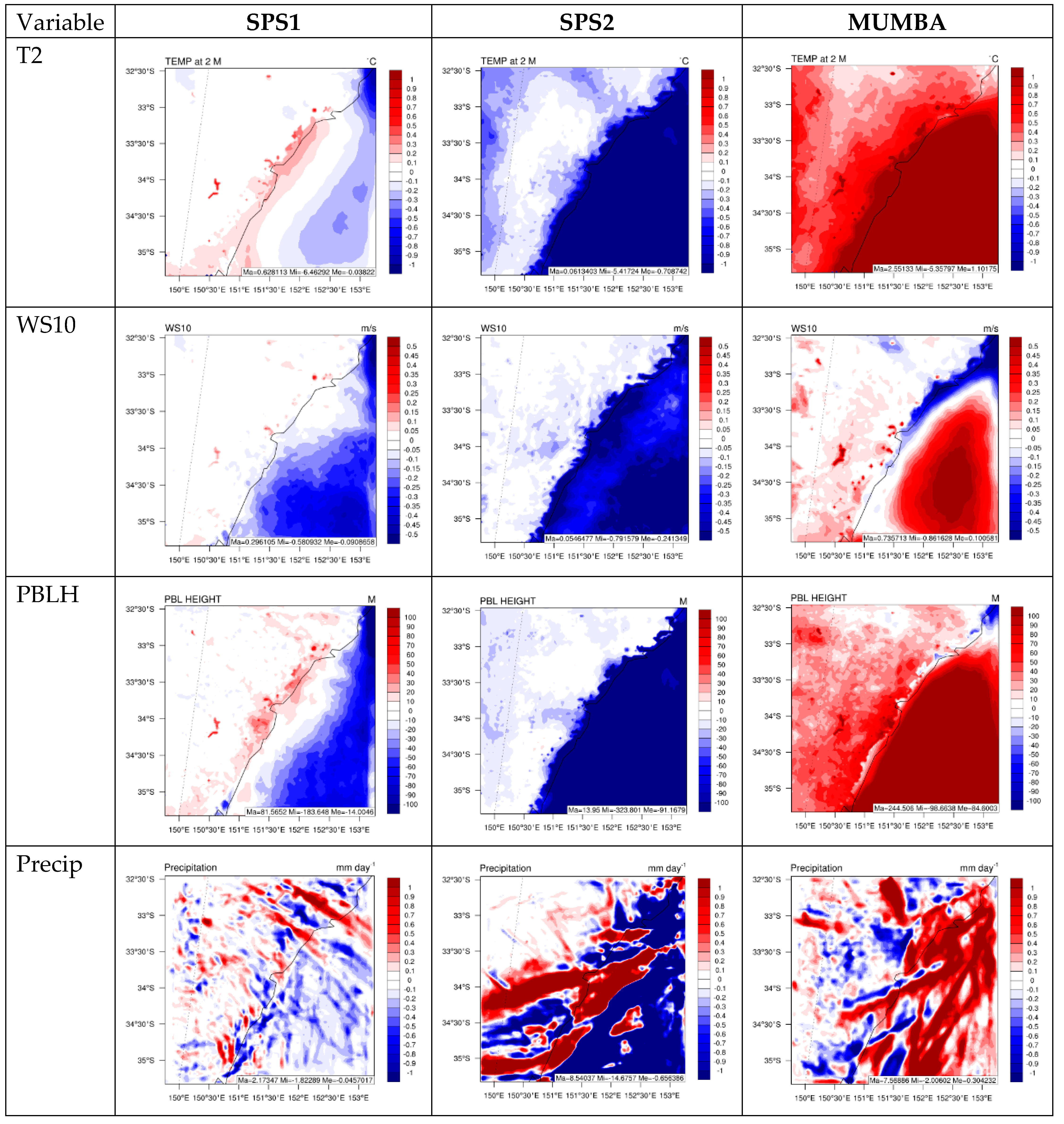
Differences in SST, LHF, and SHF between the two models lead to differences in radiative and meteorological predictions. Figure S3 and Figure 5 show the absolute differences in the spatial distributions of several radiative and meteorological variables, respectively, over d04 between WRF/Chem-ROMS and WRF/Chem. Compared to predictions from WRF/Chem, net shortwave radiation predictions from WRF/Chem-ROMS are generally higher over coastal and most oceanic areas for all field campaigns, higher for MUMBA but lower for SPS2 over land, and either higher or lower over land for SPS1. The absolute and percentage differences between net shortwave radiation simulated by WRF/Chem-ROMS and WRF/Chem range from −15 to 21.8 W m⁻² and −7.3% to 18%, respectively. Downward longwave radiation predictions from WRF/Chem-ROMS are lower over coastal and most oceanic areas for SPS1 and SPS2 but higher for MUMBA, with absolute and percentage differences of −14.5 to 9.2 W m⁻² and −4.1% to 2.6%, respectively. The differences in shortwave cloud forcing predictions between the two models are the opposite to those in net shortwave radiation, because WRF/Chem-ROMS tends to give lower cloud fractions over oceanic and coastal areas, which increases net shortwave radiation and reduces shortwave cloud forcing in those areas. The absolute differences in shortwave cloud forcing are from −21.0 to 13.1 W m⁻². Most percentage differences in shortwave cloud forcing are within ±20%. The differences in 2 m temperature (T2) predictions between the two models are driven mainly by changes in SHF, LHF, and downward longwave radiation over oceanic areas but changes in LHF and net shortwave radiation over land areas. The absolute and percentage differences in T2 range from −5.4 to 2.6 °C and −31.7% to 13.1%, respectively. The patterns of differences in predictions of 10 m wind speed (WS10) and PBLH between the two models generally follow those in T2 predictions. The absolute and percentage differences in WS10 range from −0.9 to 0.7 m s⁻¹ and −15.2% to 30.8%, respectively. The absolute and percentage differences in PBLH range from −323 to 244 m and −37.3% to 73.1%, respectively. For MUMBA, the increases in LHF and SHF deepen the PBLH, particularly over the ocean, and increase the formation of convective clouds. The opposite occurs for SPS1 and SPS2, because of decreased LHF and SHF. The absolute differences in precipitation predictions occur in either direction with a range of −14.7 to 8.5 mm day⁻¹, and most percentage differences are within ±50%. The simulated precipitation is generally higher over land areas for SPS1 and SPS2 but oceanic areas for MUMBA by WRF/Chem-ROMS than by WRF/Chem.

Table 4, Table 5 and Table 6 also compare MBs and NMBs between the two models for radiative and cloud variables. For SPS1, the performance statistics for radiative and cloud variables against satellite retrievals are overall very similar for all simulations at different grid resolutions, despite slightly worse performance for WRF/Chem-ROMS. For SPS2, WRF/Chem-ROMS gives slightly worse performance for net shortwave radiation, downward longwave radiation, shortwave and longwave cloud forcing, cloud optical thickness, cloud condensation nuclei, cloud liquid water path, and but better performance for cloud fraction and precipitating water vapor over Greater Sydney area. For MUMBA, WRF/Chem-ROMS gives slightly worse performance for downward longwave radiation, shortwave cloud forcing, cloud fraction, cloud liquid water path, and precipitating water vapor, but better performance for net shortwave radiation, longwave cloud forcing, cloud optical thickness, and cloud condensation nuclei over d04. Table 1, Table 2 and Table 3 compare MBs and NMBs between the two models for meteorological variables. For T2, comparing to domain-mean MBs from WRF/Chem, MBs from WRF/Chem-ROMS are lower at all grid resolutions except at 3 km for SPS1 and except at 81 and 9 km for SPS2 (similar at other grid resolutions for both SPS1 an SPS2), and much lower at all grid resolutions for MUMBA. For 2 m relative humidity (RH2), MBs from WRF/Chem-ROMS are lower at all grid resolutions for SPS2 and MUMBA and similar at all grid resolutions for SPS1. For WS10, MBs from WRF/Chem-ROMS are lower at all grid resolutions for SPS2 and at all grid resolutions except for 81km for MUMBA and similar at all grid resolutions for SPS1 and at 81km for MUMBA. For 10 m wind speed (WD10), MBs from WRF/Chem-ROMS are lower at all resolutions except 27 km and 9 km for SPS1, at all resolutions except 9 km for SPS2, and at 81 km for MUMBA, and similar at all other grid resolutions for those field campaigns. For precipitation against observations, MBs from WRF/Chem-ROMS are lower at all grid resolutions except at 9 km for SPS1, except at 81 km for SPS2, and except at 27 and 3 km for MUMBA, and similar at all other grid resolutions for all field campaigns. The largest improvement occurs for SPS2, reducing NMBs of precipitation against OBS from −46.7% to −31.3% at 3 km, from −44.0% to −30.2% at 9 km, and from −32.9% to −12.1% at 27 km. For precipitation against observations from the Multi-Source Weighted-Ensemble Precipitation (MSWEP), MBs from WRF/Chem-ROMS are lower at 3 km for SPS1, and at all grid resolutions except at 81 km for SPS2, and at 81 and 9 km for MUMBA. The largest improvement also occurs for SPS2, reducing NMBs of precipitation against MSWEP from −48.3% to −33.4% at 3 km, from −45.7% to −32.3% at 9 km, and from −35.0% to −14.8% at 27 km. For precipitation against the Global Precipitation Climatology Project (GPCP), WRF/Chem-ROMS improves the performance slightly for SPS1 and MUMBA but significantly for SPS2. Compared to WRF/Chem results, the NMB of precipitation from WRF/Chem-ROMS against GPCP data over d04 at 3, 9, and 27 km resolution during SPS2 reduces from 21.3% to −6.6%, from 27.7% to 0.3%, and from 70.0% to 23.5%, respectively.

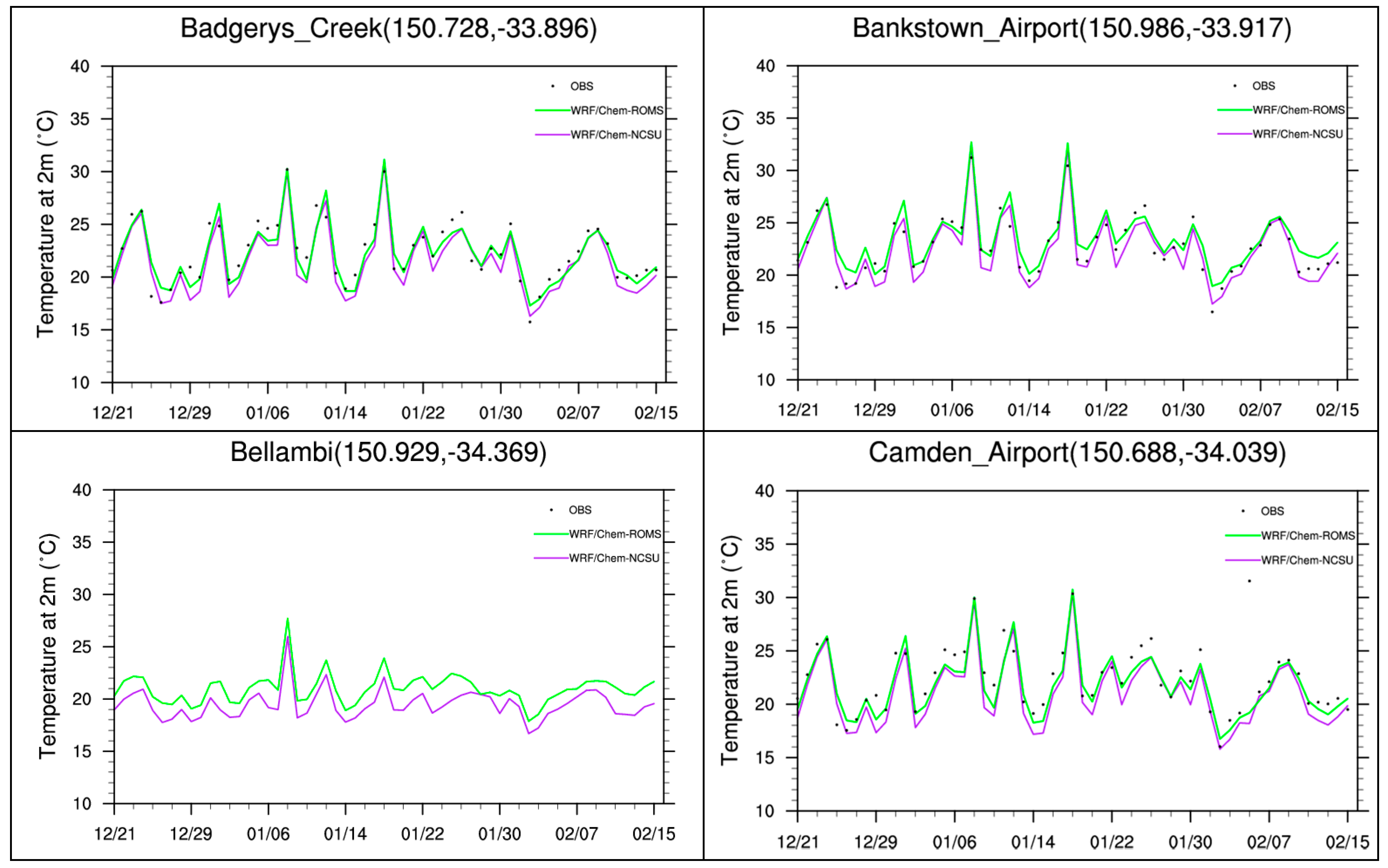
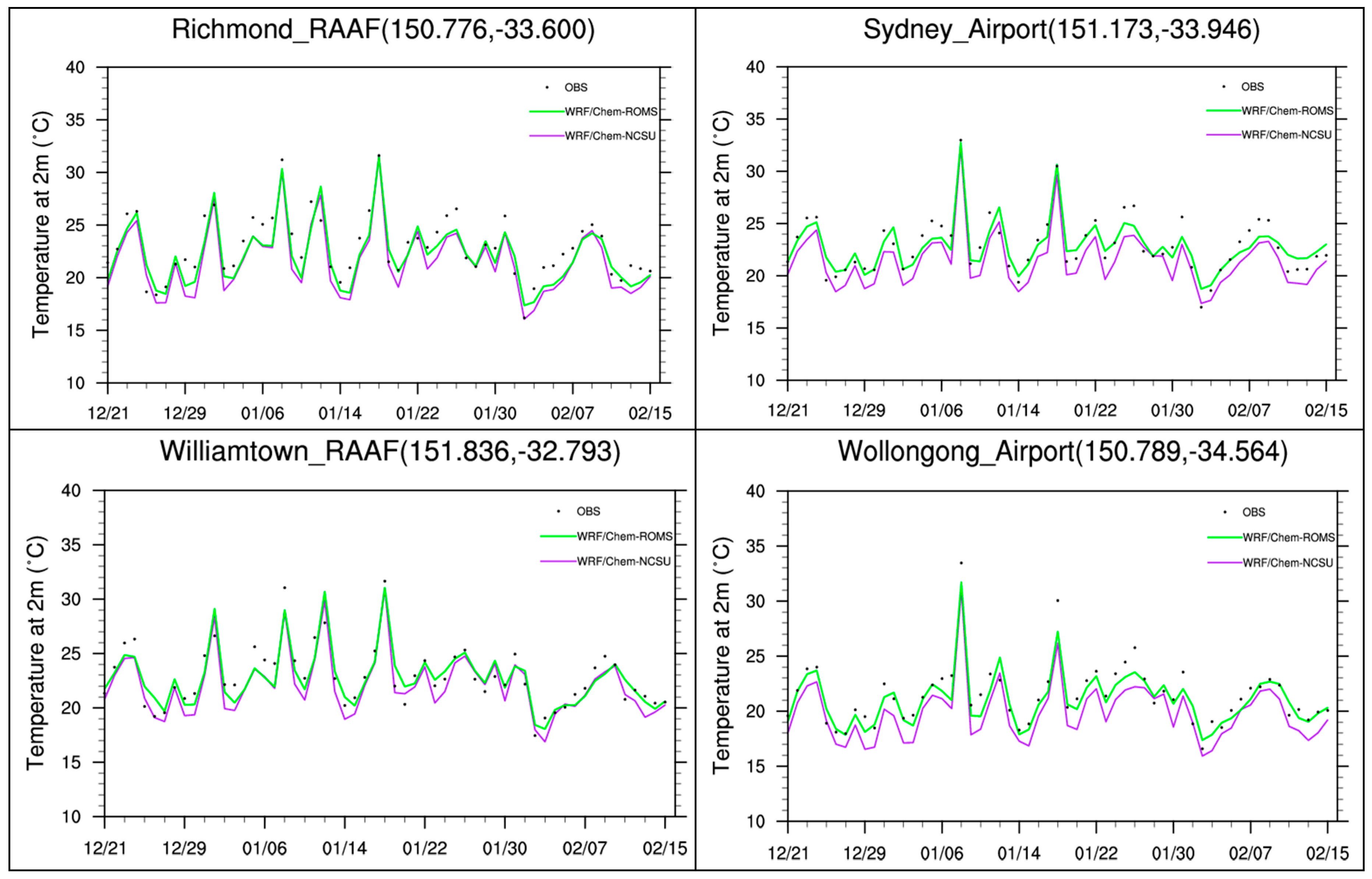
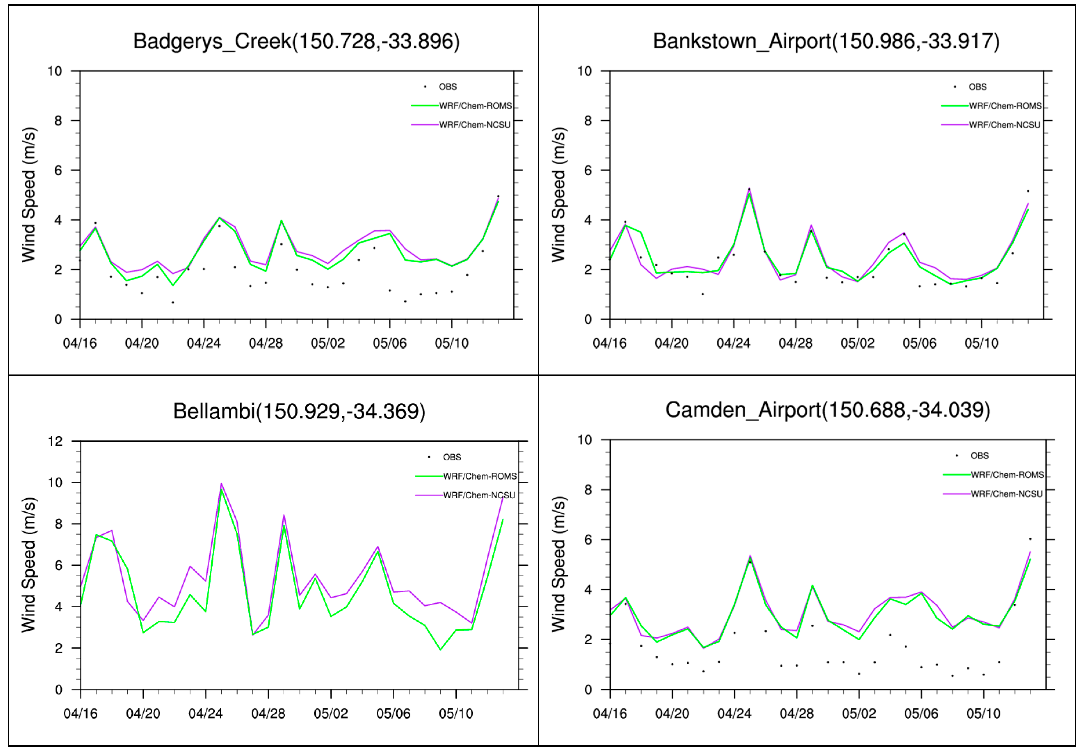
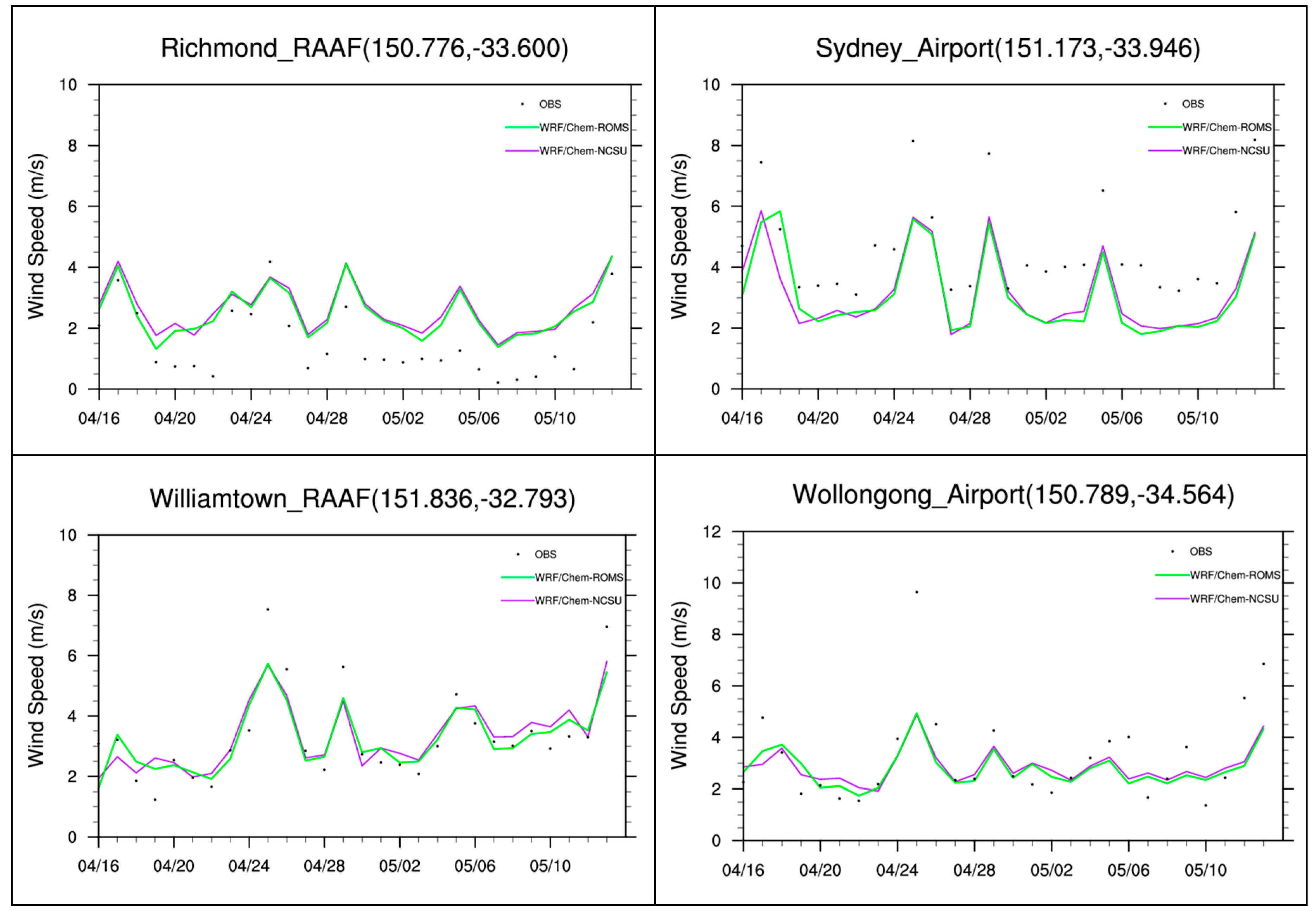
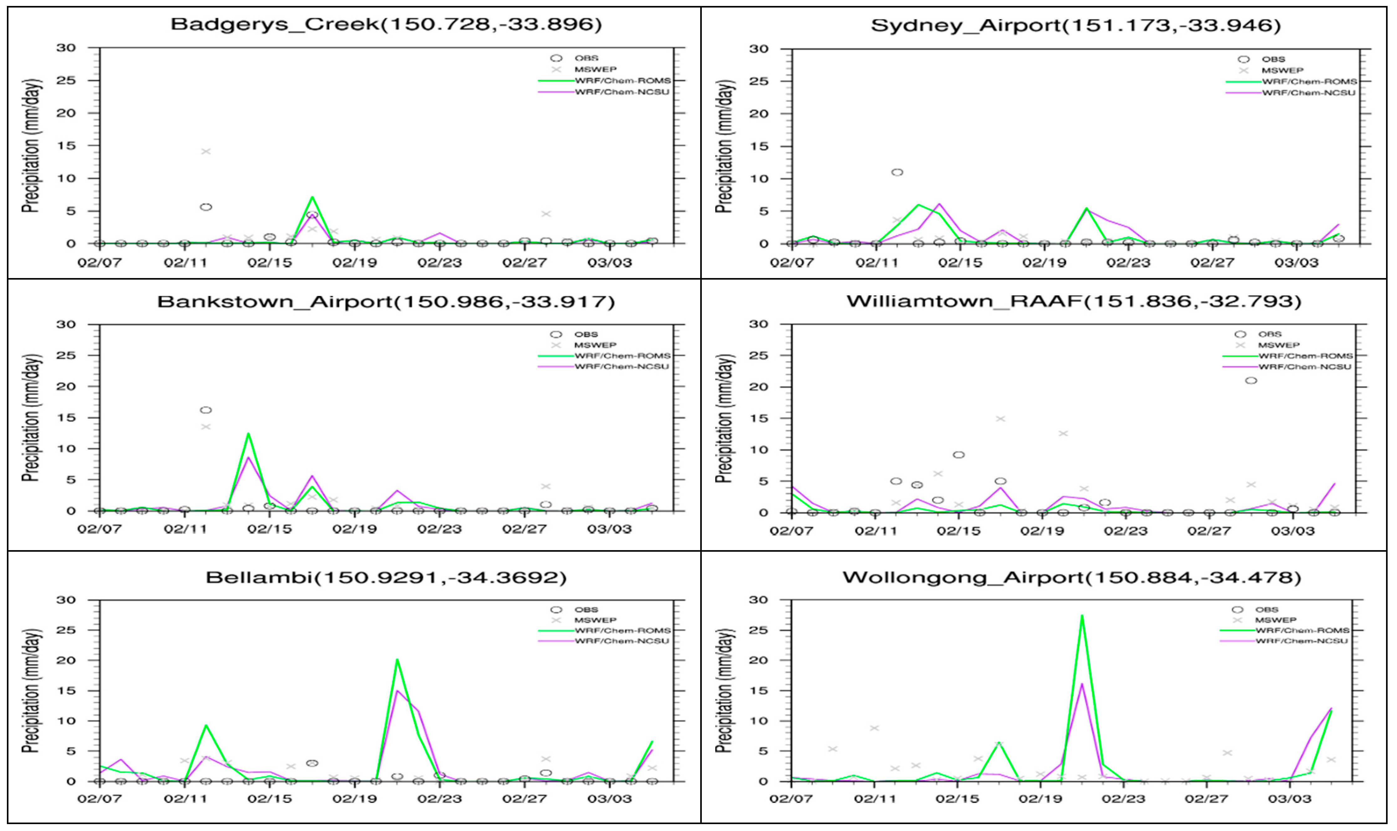
Figure 6 compares simulated temporal profiles of T2 at 8 Bureau of Meteorology (BoM) sites (i.e., Badgery’s Creek, Bankstown Airport, Bellambi, Camden Airport, Richmond RAAF, Sydney Airport, Williamtown RAAF, and Wollongong Airport) from both models against observations at 3 km resolution during MUMBA. Compared to WRF/Chem-NCSU, WRF/Chem-ROMS gives much closer agreement to observed T2 during both daytime and nighttime. This is because of more accurate predictions of SST, SHF, and LHF by WRF/Chem-ROMS. The differences between the two model predictions are generally larger at coastal sites (e.g., Sydney Airport, Bellambi, and Wollongong Airport) than at inland sites, because the T2 and other meteorological predictions are more sensitive to the differences in the air-sea interaction representation between the two models. Figure 7 compares simulated temporal profiles of WS10 at the 8 sites from both models against observations at 3 km resolution during SPS2. Compared to WRF/Chem-NCSU, WRF/Chem-ROMS generally gives less overpredictions for WS10 during most days at Badgery’s Creek, Camden Airport, Williamtown RAAF, and Wollongong Airport and some days at other sites. Figure 8 compares simulated temporal profiles of precipitation at 6 selected BoM sites from both models against observations at 3 km resolution during SPS1, SPS2, and MUMBA. During SPS1, WRF/Chem-ROMS tends to give slightly higher precipitation during several days at all sites, except for Sydney airport and Williamtown RAAF. However, its predictions agree better with observations on some days, leading to slightly smaller NMBs (3.5% vs. 8.3%) at all sites. During SPS2, WRF/Chem-ROMS captures better heavy precipitation events on 18 April 2012 at Badgery’s Creek, Bellambi, Sydney Airport, and Williamtown RAAF (−31.3% vs. −46.7%). During MUMBA, although WRF/Chem-ROMS captures better heavy precipitation events on 29 January 2013 at Sydney Airport and 2 February 2013 at all sites, particularly at Williamtown RAAF, it gives larger underpredictions for heavy precipitation events on 29 January 2013 at Badgery’s Creek, Bankstown Airport, Bellambi, and Wollongong Airport, leading to slightly larger underpredictions (NMBs of −40.7% vs. −37.2%).

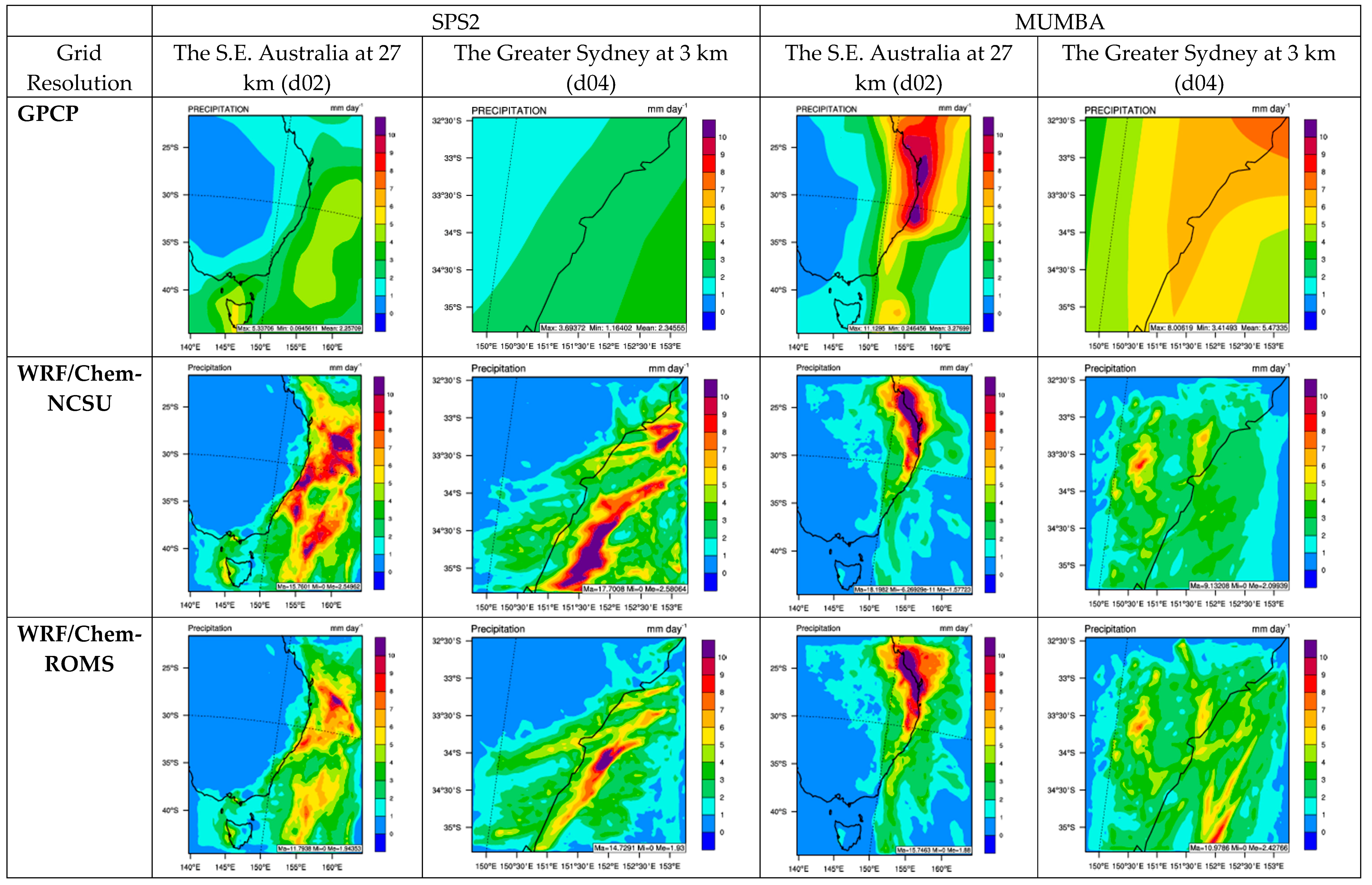
Figure 9 and Figure S4 compare the spatial distributions of simulated precipitation from both models against those from GPCP over southeastern Australia at 27 km resolution (d02) and the Greater Sydney area at 3 km resolution (d04) during SPS2 and MUMBA, respectively. During SPS2, compared to GPCP, precipitation is overpredicted with an NMB of 21.8% and 21.3% by WRF/Chem but underpredicted with an NMB of −3.7% and −6.6% by WRF/Chem-ROMS at 27 km resolution over d02 and at 3 km resolution over d04, respectively. Overpredictions occur mostly over the ocean for both models. During MUMBA, precipitation is underpredicted with an NMB of −47.1% and −56.9% by WRF/Chem and with an NMB of −37.5% and−50.7% by WRF/Chem-ROMS at 27 km resolution over d02 and at 3 km resolution over d04, respectively. As shown in Figure 9, underpredictions occur mostly over the southern portion of d02 for both models, to the lesser extent for WRF/Chem-ROMS. Underpredictions occur in some land and oceanic areas in the northern portion and some oceanic areas in the eastern portion of d04, to the lesser extent for WRF/Chem-ROMS. These results illustrate improved precipitation resulting from explicit representations of air-sea interactions through coupling of WRF/Chem and ROMS.

3.3. Chemical Predictions

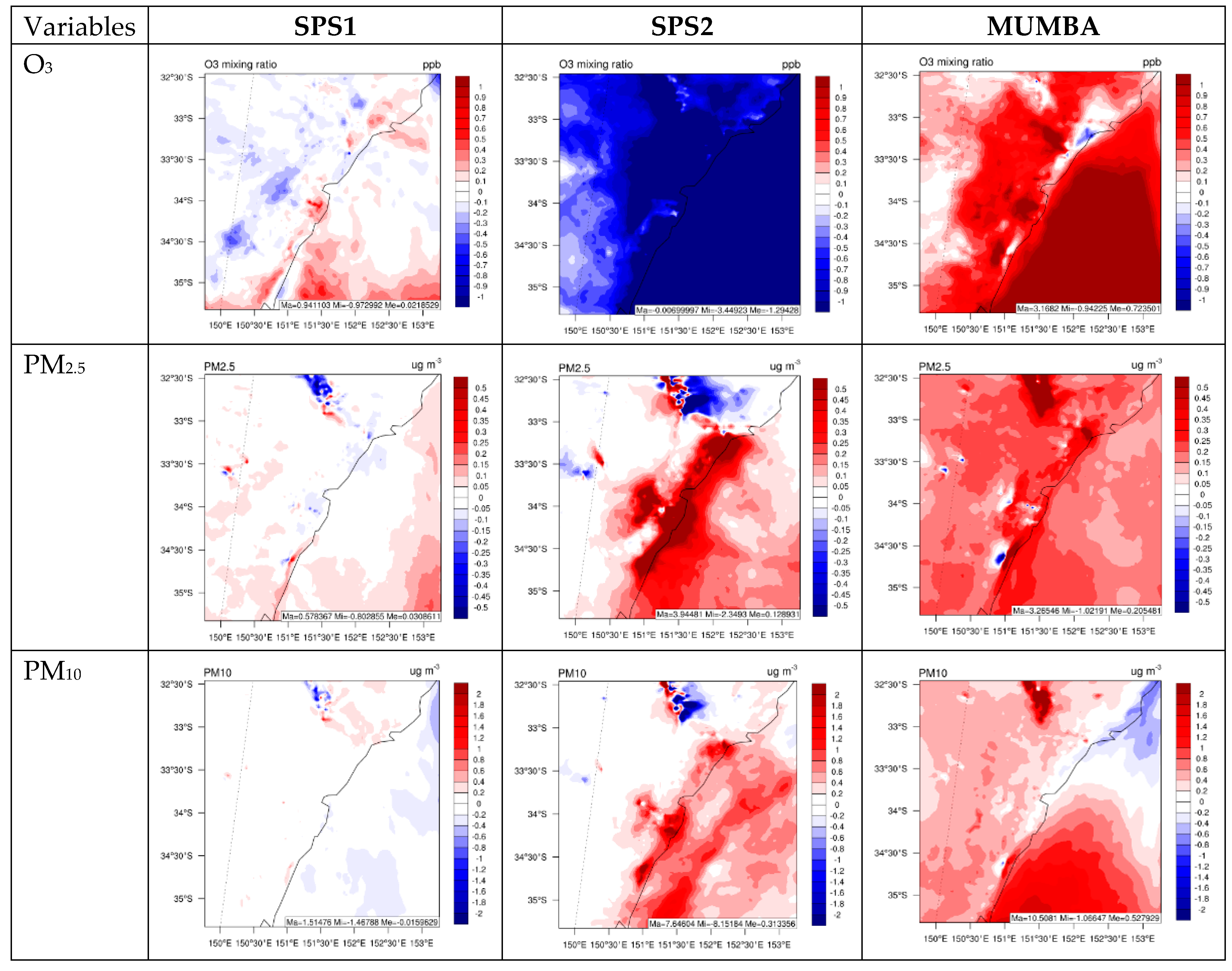
The changes in radiative and meteorological variables due to the inclusion of air-sea interactions in WRF/Chem-ROMS can affect chemical concentrations to various degrees. As an example, Figure S5 and Figure 10 show the absolute differences in the spatial distributions of CO, HCHO, isoprene, OH, O₃, PM_2.5, and PM₁₀ over d04 between WRF/Chem-ROMS and WRF/Chem during the three field campaigns. While the absolute differences are generally within 1 ppb for gaseous species, except CO whose differences may be up to 4.5 ppb, the domain-mean percentage differences are as large as 4.5% for CO, 16.1% for SO₂, 27% for NO₂, 9.8% for HCHO, 20.0% for isoprene, 17.3% for terpenes, 15.2% for H₂O₂, and 6.1% for O₃. The domain-mean absolute and percentage differences are 0.03–0.2 μg m⁻³ and 1.2–7.3% for PM_2.5, 0.02–0.5 μg m⁻³, and 0.6–7.4% for PM₁₀, respectively. The absolute and relative differences in these surface concentrations over d04 are larger than the domain mean values, for example, the percentage differences are mostly in the range of ±10% for CO, ±50% for SO₂, ±30% for NO₂, ±25% for HCHO, ±60% for isoprene, ±60% for terpenes, ±35% for H₂O₂, ±10% for OH, ±10% for O₃, ±15% for PM_2.5, and ±12% for PM₁₀. The patterns of differences are overall similar for CO, SO₂, and NO₂, for isoprene and terpenes, and for HCHO and H₂O₂. These differences reflect the net impacts of differences in radiative and meteorological variables on atmospheric chemistry and relevant processes such as dry and wet removals and atmospheric transport. For example, the increased surface CO, SO₂, and NO₂ mixing ratios in most regions may be caused mainly by the decreased PBLH and OH radicals for SPS2 and the decreased OH radicals for MUMBA. The isoprene mixing ratios increase for SPS1 and MUMBA and decrease for SPS2, which are the responses to the increased T2 for SPS1 and MUMBA and decreased T2 for SPS2. The increased HCHO mixing ratios for SPS1 and MUMBA and the decreased HCHO mixing ratios for SPS2 over land areas are caused by the similar changes in the isoprene mixing ratios. Those over oceanic areas are mainly caused by changes in PBLH and T2. The changes in meteorological variables such as T2, WS10, PBLH, and precipitation and the concentrations of precursors such as HCHO, isoprene, NO₂, and CO cause the changes in surface O₃ mixing ratios.

For all field campaigns, the concentrations of PM_2.5 simulated by WRF/Chem-ROMS are higher than those by WRF/Chem over most regions, resulting from high SO₄²⁻ and NH₄⁺ over ocean and higher NO₃⁻, EC, and OC over both land and ocean. The changes in WS10 can affect the emissions of sea-salt particles, which will in turn affect PM₁₀ concentrations. The correlation of changes in WS10 and changes in PM₁₀ concentrations is strong for MUMBA, because the impact of WS10 dominates over the impacts of other factors for simulated PM₁₀ concentrations. The increased PM₁₀ in the coastal areas and ocean for SPS2 is mainly caused by increased PM_2.5 and decreased PBLH. For SPS1, despite increased PM_2.5 and decreased PBLH, PM₁₀ concentrations decrease slightly mainly because of decreased sea-salt particles resulted from reduced WS10.

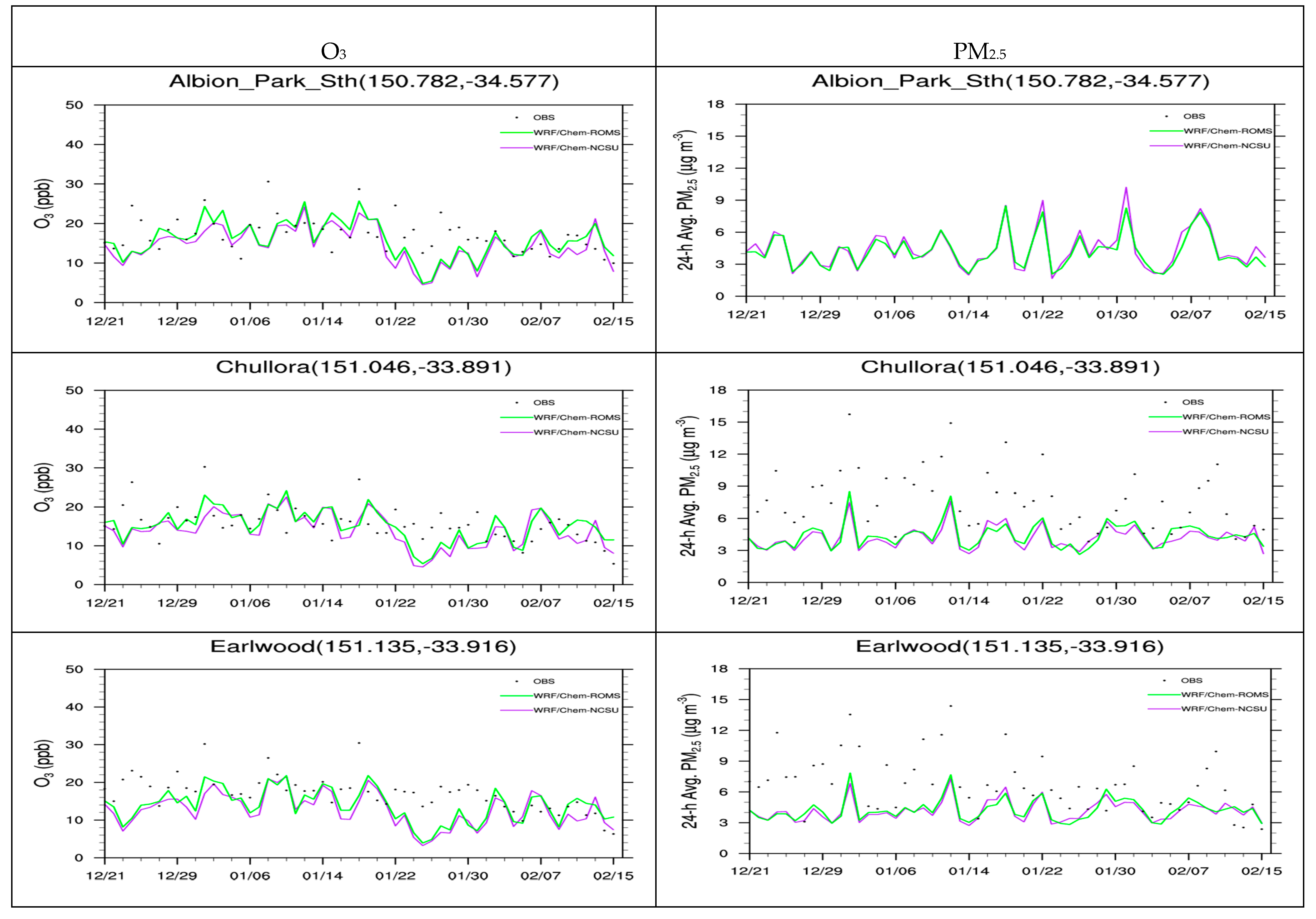
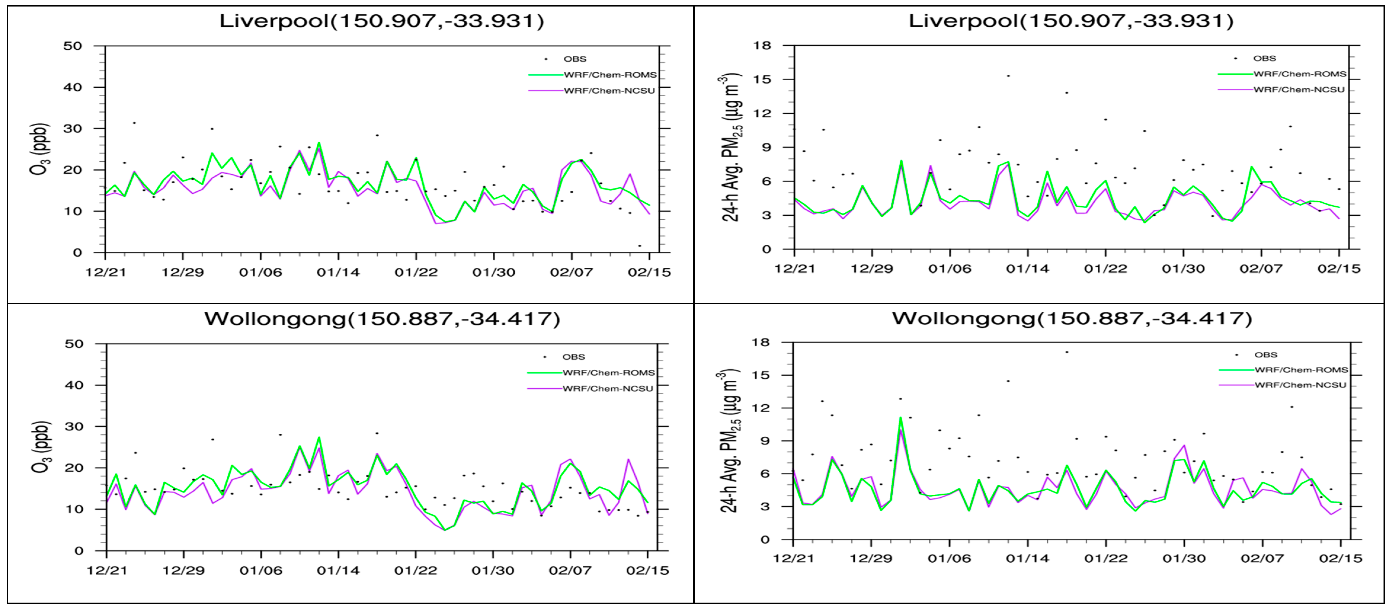
As shown in Table 1, Table 2 and Table 3, the statistical performance of WRF/Chem-ROMS at 3 km resolution in d04 is slightly better for CO, NO, PM_2.5, and PM₁₀ for SPS1, CO, O₃, and PM₁₀ for SPS2, and NO, NO₂, O₃, PM_2.5, and, PM₁₀ for MUMBA. Figure 11 compares the temporal variation of simulated daily-average surface concentrations of O₃ and PM_2.5 by WRF/Chem-NCSU and WRF/Chem-ROMS at 3 km at selected sites during MUMBA. Compared to WRF/Chem-NCSU, higher temperatures, biogenic VOCs, HCHO, and CO by WRF/Chem-ROMS lead to higher predicted O₃ concentrations during most days, bringing O₃ predictions into better agreement with observations at all sites (NMBs of −10.1% vs. −15.6%). The role of biogenic VOCs in enhancing surface O₃ in Greater Sydney area has been reported in Utembe et al. [23]. Simulated PM_2.5 concentrations from WRF/Chem-ROMS are also slightly higher during most days at all sites because of higher temperature, higher BVOCs and SO₂, and lower precipitation predictions, which slightly improves the model performance (NMBs of −43.6% vs. −45.6%).

As shown in Table 4, Table 5 and Table 6, WRF/Chem-ROMS gives slightly better performance for column NO₂ and HCHO for SPS1, column NO₂ and TOR for SPS2, and column CO, NO₂ (at 3 km resolution only), and HCHO for MUMBA. NMBs for AOD are slightly lower for WRF/Chem-ROMS at all grid resolutions during SPS1 and at 81 and 27 km resolution during SPS2 but slightly higher at all grid resolutions during MUMBA. AOD predictions from WRF/Chem-ROMS are slightly higher over most areas for SPS2 and MUMBA and over land areas for SPS1 (Figures not shown), mainly caused by differences in column PM_2.5 concentrations.

4. Impact of Chemical Boundary Conditions

Table 7. Normalized mean biases (NMBs) (%) of chemical predictions from WRF/Chem simulations without (top) and with (bottom) adjusted boundary conditions at 81 km (d01), 27 km (d02), 9 km (d03), and 3 km (d04) over the 3 km domain (d04).

a. Without Adjusted Boundary Conditions

Variables

SPS1

SPS2

MUMBA

d01

d02

d03

d04

d01

d02

d03

d04

d01

d02

d03

d04

Column

AOD

2.7

6.4

8.3

7.1

87.4

75.3

83.8

66.0

34.2

27.3

40.6

27.5

CO

−31.1

−30.8

−30.7

−30.5

−25.4

−25.0

−25.1

−24.9

−26.4

−26.1

−26.0

−25.9

NO2

−41.8

−31.2

−25.8

−24.1

−38.5

−27.9

−25.6

−23.3

−29.0

−20.3

−17.3

−14.3

HCHO

−17.1

−20.9

−22.9

−21.9

−21.6

−24.1

−24.6

−22.6

8.9

2.9

−1.0

0.9

TOR

12.5

11.0

9.8

9.1

−9.1

−9.4

−10.0

−9.9

−6.9

−8.0

−8.6

−9.0

Chem

O3 (ppb)

0.3

−15.4

−21.3

−21.3

13.7

−7.5

−15.4

−9.2

−12.9

−28.0

−34.8

−37.8

CO (ppb)

−66.1

−53.8

−58.9

−46.3

−61.7

−36.5

−37.7

−33.0

−55.1

−41.3

−43.8

−20.0

NO (ppb)

−80.1

−24.2

−0.4

17.8

−90.4

−48.4

−1.4

4.9

−59.1

28.5

65.1

129.4

NO2 (ppb)

−34.0

−5.3

−2.6

3.2

−33.6

−4.0

9.9

12.6

−26.5

7.0

11.6

22.1

SO2 (ppb)

44.7

87.7

87.4

108.7

71.6

127.0

122.0

141.4

39.6

80.2

97.7

149.0

PM2.5 (μg m−3)

−41.8

−32.1

−29.7

−25.9

−7.3

37.9

102.4

134.5

−60.0

−52.7

−50.0

−46.7

PM10 (μg m−3)

−60.2

−57.2

−56.6

−54.2

−35.0

−29.7

−15.5

−8.9

−64.4

−60.3

−59.2

−55.2

b. With Adjusted Boundary Conditions

Variables

SPS1

SPS2

MUMBA

d01

d02

d03

d04

d01

d02

d03

d04

d01

d02

d03

d04

Column

AOD

3.1

7.2

9.2

7.9

73.9

76.7

70.5

66.4

23.7

27.7

28.8

27.8

CO

−22.0

−21.7

−21.6

−21.3

−7.3

−7.0

−7.0

−6.8

−17.5

−17.2

−17.2

−17.1

NO2

−42.6

−31.2

−24.8

−23.2

−37.6

−26.3

−23.2

−21.2

−29.5

−20.1

−15.2

−12.4

HCHO

−17.0

−20.8

−22.8

−21.9

−23.1

−25.4

−25.8

−24.1

−5.0

−9.6

−13.2

−11.8

TOR

26.9

25.1

23.8

23.0

5.9

5.6

5.1

5.1

41.8

40.4

39.9

39.0

Chem

O3 (ppb)

16.4

−0.1

−5.8

−5.7

30.7

7.0

−1.9

4.9

8.5

−5.6

−12.4

−15.6

CO (ppb)

−63.6

−51.3

−56.3

−44.5

−58.9

−34.0

−35.2

−30.2

−52.2

−38.7

−41.1

−18.2

NO (ppb)

−83.9

−32.4

−10.8

6.5

−91.8

−51.9

−7.1

−0.1

−68.9

2.0

31.4

86.9

NO2 (ppb)

−32.8

−1.4

2.5

9.3

−32.8

−0.0

15.1

18.2

−23.6

16.4

25.0

38.7

SO2 (ppb)

46.0

93.5

87.9

110.2

71.3

126.8

123.3

141.4

37.4

80.5

99.4

146.6

PM2.5 (μg m−3)

−41.0

−29.9

−28.4

−25.2

−5.0

41.0

104.6

137.9

−58.6

−51.0

−48.5

−45.6

PM10 (μg m−3)

−59.8

−55.6

−55.9

−53.8

−33.5

−28.3

−14.5

−7.0

−63.7

−59.6

−58.5

−54.7

AOD: aerosol optical depth; CO: carbon monoxide; NO₂: nitrogen dioxide; HCHO: formaldehyde; TOR: tropospheric ozone residual; O₃: ozone; CO: carbon monoxide; NO: nitric oxide; NO₂: nitrogen dioxide; SO₂: sulfur dioxide; PM_2.5 and PM₁₀: particulate matter with aerodynamic diameters ≤2.5 μm and 10 μm; SPS1 and SPS2: Sydney Particle Study Stages 1 and 2; MUMBA: the Measurements of Urban, Marine and Bioge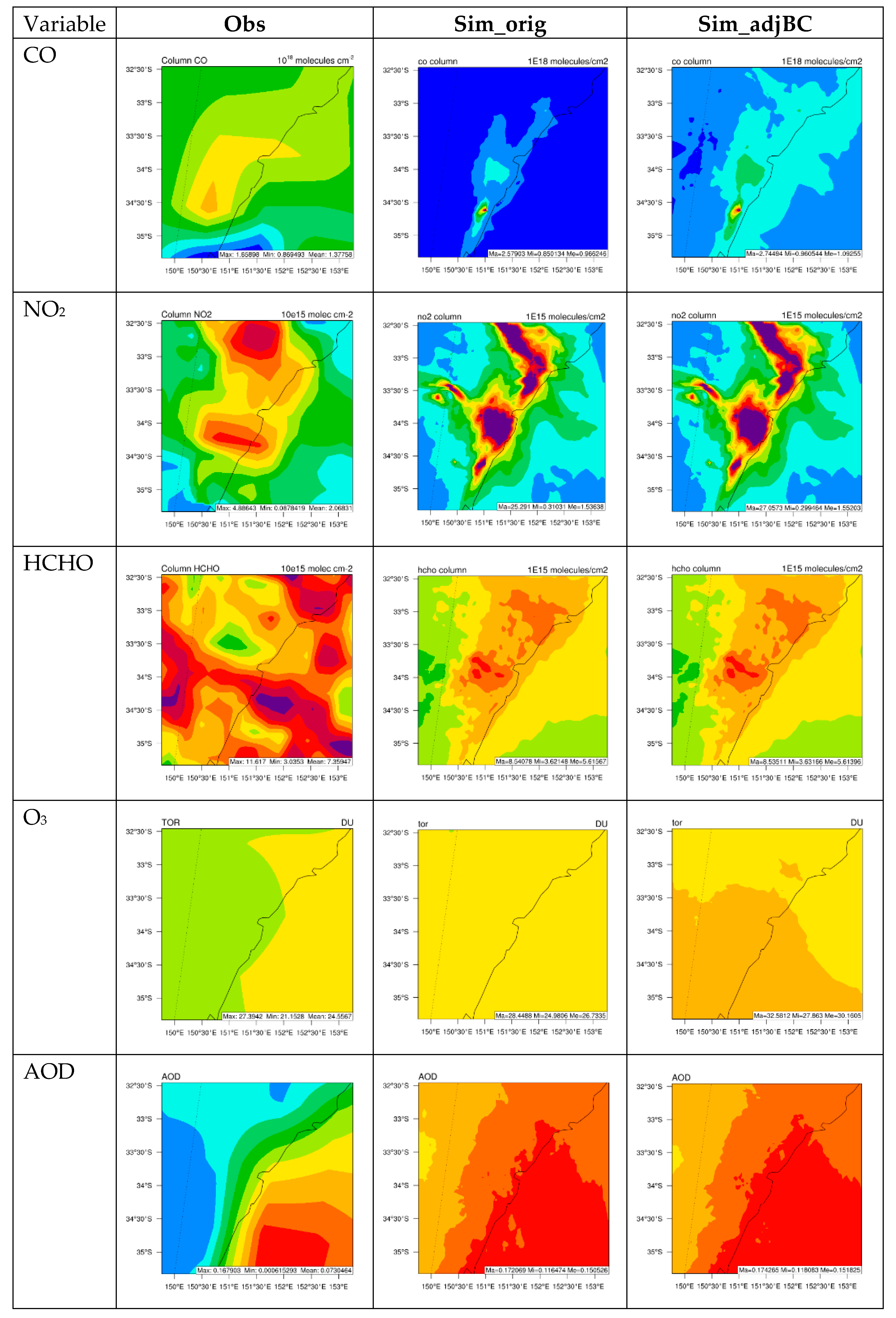nic Air.

summarizes the normalized mean biases (NMBs) of column and surface chemical predictions from WRF/Chem simulations without and with adjusted BCONs at 81 km (d01), 27 km (d02), 9 km (d03), and 3 km (d04) over the 3 km domain (d04). Figure 12 and Figure S6 compare satellite observed column mass abundances of gases and AOD with those simulated by WRF/Chem-NCSU without and with adjustment of BCONs over Greater Sydney (d04) during SPS1 and SPS2, respectively. The predictions from WRF/Chem-ROMS without and with adjustment of BCONs are similar to those from WRF/Chem-NCSU, thus not shown here. Among all the column variables, the spatial distributions and magnitudes of column CO with adjusted BCONs are obviously improved over all domains. The NMBs in d01 reduce largely from −31.1% to −22.0% for SPS1, from −25.4% to −7.3% for SPS2, and from −26.4% to −17.5% for MUMBA. Similar improvements are found for model predictions at all finer grid resolutions. For example, the NMBs of column CO predictions in d04 reduce largely from −30.5% to −21.3% for SPS1, from −24.9% to −6.8% for SPS2, and from −25.9% to −17.1% for MUMBA. For column NO₂, NMBs with adjusted BCONs are slightly worse at 81, 27, and 9 km, but slightly better at 3 km for SPS1, slightly better at all grid resolutions for SPS2, and slightly worse at 81km, but slightly better at other finer grid resolutions for MUMBA. For example, the NMBs in d04 reduce slightly from −24.1% to −23.2% for SPS1, from −23.3% to−21.2% for SPS2, and from −14.3% to −12.4% for MUMBA. The simulated spatial distributions for column NO₂ without and with adjusted BCONs are similar, both simulations capture well the hot spots but tend to overpredict the values of these hot spots, but underpredict column NO₂ in other regions. For column HCHO, NMBs are slightly better at all grid resolutions for SPS1 and MUMBA and slightly worse at all grid resolutions for SPS2. The spatial distributions for column HCHO without and with adjusted BCONs are very similar for all field campaigns, with moderate underpredictions for SPS1 and SPS2 and slight underpredictions for MUMBA. For column O₃, NMBs with adjusted BCONs are slightly better for SPS2 but worse for SPS1 and MUMBA. The spatial distributions of simulated column O₃ without and with adjusted BCONs do not agree with the satellite observations, with slight overpredictions for SPS2 but moderate overpredictions for SPS1 and MUMBA. The O₃ lateral boundary condition is adjusted using a fixed factor throughout all altitudes for each boundary side. More accurate adjustments by considering the shape of O₃ profiles (i.e., altitude weighted adjustment factors) need to be considered in the future work. For AOD, NMBs are better at all grid resolutions for SPS1 and at 81 km and 27 km for SPS2, but slightly worse at all grid resolutions for MUMBA.

The adjusted chemical BCONs can affect surface concentration predictions. For example, NMBs of surface CO and NO predictions over d04 reduce from −46.3% to −44.5% and 17.8% to 6.5% for SPS1, from −33.0% to −30.2%, and 4.9% to −0.1% for SPS2, and from −20.0% to −18.2% and 129.4% to 87.9% for MUMBA, respectively. NMBs of surface O₃ predictions at 3 km resolution over d04 reduce from −21.3% to −5.8% for SPS1, from −9.2% to 4.9% for SPS2, and from −37.8% to −15.6% for MUMBA. NMBs of surface PM_2.5 predictions at 3 km over d04 are slightly better for SPS1 and MUMBA and those of surface PM₁₀ predictions are slightly better over d04 at all grid resolutions. Figure S7 compares observed temporal variations of surface CO mixing ratios with two sets of surface CO predictions from WRF/Chem-NCSU at 3 km resolution at selected sites during SPS1; one using CO BCONs derived from CESM-NCSU simulations and one using CO BCONs constrained by satellite data. Slight improvement in surface CO predictions is found at all sites.

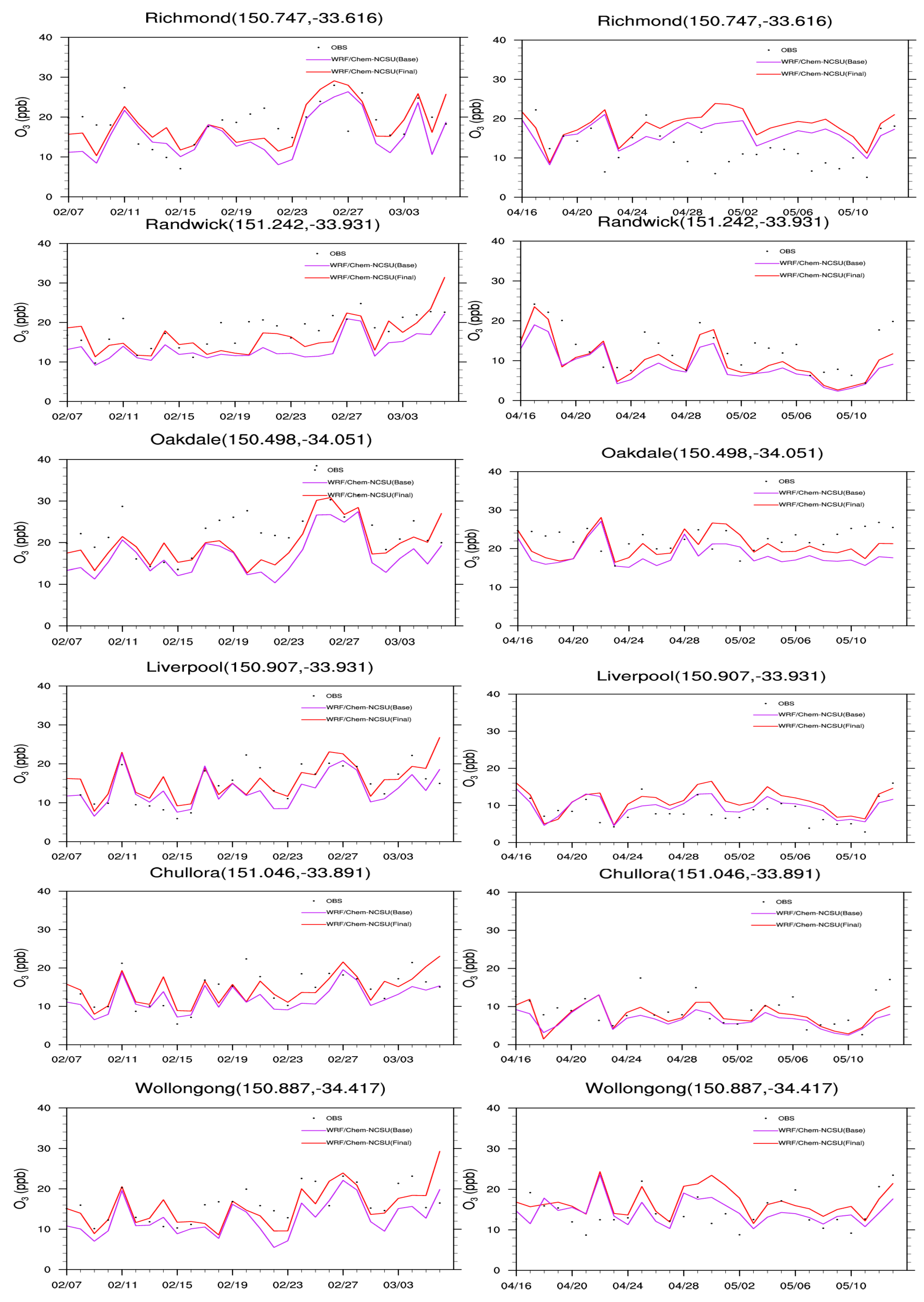
Figure 13 compares observed temporal variations of surface O₃ mixing ratios with two sets of O₃ predictions from WRF/Chem-NCSU at 3 km at selected sites during SPS1 without and with adjusted O₃ BCONs. Using satellite-constrained chemical BCONs for O₃ appreciably improves the performance of O₃ during most days at all sites. Compared to several studies on the importance of chemical BCONs over North America [9,11], the magnitude of relative changes in surface O₃ concentrations due to changes in chemical BCONs of O₃ is larger in Australia. For example, Yahya et al. [11] reported changes in the range of NMBs for maximum 8 h mixing ratios from −11.8% to −5.6% in 2006 and −13.0% to −11.1% in 2010 at rural sites and from −2.8% to −1.7% in 2006 and −1.1% to −7.0% in 2010 at urban and suburban sites in the continental U.S., when changing the chemical BCONs based on results from one global model to another. These relative changes are much smaller than those in this work (e.g., adjusted BCONs reduce NMBs of surface O₃ concentrations from −21.3% to −5.8% for SPS1 and from −37.8% to −15.6% for MUMBA) because of lower surface O₃ levels in Australia than those over North America, indicating a more important role of chemical BCONs in the Southern Hemisphere compared to the Northern Hemisphere.

5. Conclusions

As described in the Part I paper, the only difference between WRF/Chem and WRF/Chem-ROMS lies in the fact that air-sea interactions are not treated in WRF/Chem, but are explicitly represented in WRF/Chem-ROMS through a dynamic atmosphere-ocean coupling. As a result, SST is simulated in WRF/Chem-ROMS but prescribed based on RTG_SST analysis data in WRF/Chem. In this Part II paper, the results from WRF/Chem are evaluated using surface observations from the three field campaigns, satellite retrievals, and combined satellite and reanalysis data and compared with those of WRF/Chem-ROMS to assess the impact of air-sea interaction representation on meteorological and chemical predictions. A second objective of this Part II paper is to assess the impact of chemical BCONs used on overall model predictions.

At spatial grid resolutions of 3, 9, and 27 km, compared to WRF/Chem, the explicit air-sea interactions in WRF/Chem-ROMS lead to substantial improvements in terms of performance statistics and spatial distributions in the model’s predictability of sea-surface temperature, latent heat fluxes, and sensible heat fluxes over the ocean. For example, the MBs of SST are within ±1 °C for WRF/Chem-ROMS but can be up to ±3.3 °C for WRF/Chem during all three field campaigns. WRF/Chem-ROMS assembles the spatial distributions and gradients of SST, LHF, and SHF much closer to those from OAFlux. The use of finer grid resolutions (3 or 9 km) effectively reduces the biases in SST, LHF, and SHF during SPS1 and SPS2 by WRF/Chem-ROMS, whereas it further increases these biases for WRF/Chem during all field campaigns.

The large differences in SST, LHF, and SHF between the two models lead to different radiative, cloud, and meteorological predictions. For example, over the Greater Sydney area, the percentage differences between WRF/Chem-ROMS and WRF/Chem are −7.3% to 18% for net shortwave radiation, −4.1% to 2.6% for downward longwave radiation, −31.7% to 13.1% for T2, −15.2% to 30.8% for WS10, −37.3% to 73.1% for PBLH, and as large as ±20% for shortwave cloud forcing and ±50% for precipitation. While WRF/Chem-ROMS gives either similar or slightly worse performance for most radiative and cloud variables, it generally gives better performance in terms of performance statistics and temporal variations for meteorological predictions such as T2, RH2, WS10, WD10, and precipitation, with a few exceptions. For example, during SPS2, the WRF/Chem-ROMS simulation at 3 km reduces NMBs of precipitation from −46.7% to −31.3%, from −48.3% to −33.4%, and from 21.3% to −6.6% against data from OBS, MSWEP, and GPCP, respectively. WRF/Chem-ROMS also better captured heavy precipitation events on 18 April 2012 at Badgery’s Creek, Bellambi, Sydney Airport, and Williamtown RAAF during SPS2 and 29January 2013 at Sydney Airport and 2 February 2013 at all sites during MUMBA.

The differences in radiative, cloud, and meteorological predictions, in turn, cause different chemical predictions. For example, compared to WRF/Chem results, the decreased PBLH from WRF/Chem-ROMS may explain in part the increased surface CO, SO₂, and NO₂ mixing ratios in most regions during SPS2. The increased T2 for SPS1 and MUMBA from WRF/Chem-ROMS lead to higher isoprene and, thus, higher HCHO mixing ratios over land areas. The opposite occurs for SPS2. The changes in WS10 simulated by WRF/Chem-ROMS can affect the emissions of sea-salt particles, which in turn affect PM₁₀ concentrations. As a result, the percentage differences in surface concentrations are mostly in the range of ±10% for CO, OH, and O₃, ±25% for HCHO, ±30% for NO₂, ±35% for H₂O₂, ±50% for SO₂, ±60% for isoprene and terpenes, ±15% for PM_2.5, and ±12% for PM₁₀. Compared to WRF/Chem, WRF/Chem-ROMS can increase the concentrations of O₃, PM_2.5, and PM₁₀ by up to 3.1 ppb, 3.9 μg m⁻³, and 10.1 μg m⁻³, and decrease them as large as 3.4 ppb, 2.3 μg m⁻³, and 8.2 µg m⁻³, with domain-mean changes of −1.3 to 0.7 ppb (−6.1% to 4.0%), 0.03–0.2 µg m⁻³ (1.2–7.3%), and 0.02–0.5 μg m⁻³ (0.6-7.4%), respectively, for O₃, PM_2.5, and PM₁₀. The WRF/Chem-ROMS simulations at 3 km resolution slightly improves the statistical performance of surface concentrations of CO, NO, PM_2.5, PM₁₀, column NO₂ and HCHO for SPS1, CO, O₃, PM₁₀, column NO₂, and TOR for SPS2, and NO, NO₂, O₃, PM_2.5, PM₁₀, and column CO, NO₂ and HCHO for MUMBA.

The BCONs of CO, NO₂, HCHO, O₃, and PM_2.5 are constrained based on satellite retrievals of column CO, NO₂, HCHO, O₃, and AOD, respectively. Compared to WRF/Chem simulations without adjusted BCONs, WRF/Chem simulations with satellite-constrained BCONs improve the spatial distributions and magnitudes of column CO at 81 km over d01, which leads to improvement at 27, 9, and 3 km in d04. For example, the NMBs of column CO predictions in d04 reduce largely from −30.5% to −21.3% for SPS1, from −24.9% to −6.8% for SPS2, and from −25.9% to −17.1% for MUMBA. The use of satellite-constrained BCONs also slightly improves the performance of column NO₂ for SPS1 and SPS2, column HCHO for SPS1 and MUMBA, and TOR for SPS2 at 3 km resolution over d04. The adjusted BCONs reduce the NMBs of surface CO, NO, and O₃ predictions at 3 km over d04 from −46.3% to −44.5%, from 17.8% to 6.5%, and from −21.3% to −5.8% for SPS1, from −33.0% to −30.2%, from 4.9% to −0.1%, and from −9.2% to 4.9% for SPS2, and from −20.0% to −18.2%, from 129.4% to 87.9%, and from −37.8% to −15.6% for MUMBA, respectively. They reduce slightly the NMBs of surface PM_2.5 predictions at 3 km resolution over d04 for SPS1 and MUMBA and those of surface PM₁₀ predictions at all grid resolutions for all field campaigns. Compared to results from past studies on the impact of chemical BCONs on surface O₃ concentrations over North America, the magnitude of relative changes in surface O₃ concentrations due to changes in chemical BCONs of O₃ reported in this work is larger because of lower surface O₃ levels in Australia than those in North America. This indicates a more important role of chemical BCONs in the Southern Hemisphere compared to the Northern Hemisphere and, thus, a crucial need for more realistic chemical BCONs of O₃ in the relatively clean Southern Hemisphere.

References

1. Nelson, J.; He, R. Effect of the Gulf Stream on winter extratropical cyclone outbreaks. Atmos. Sci. Lett. 2012, 13, 311–316. [Google Scholar] [CrossRef]
2. Nelson, J.; He, R.; Warner, J.C.; Bane, J. Air–sea interactions during strong winter extratropical storms. Ocean Dyn. 2014, 64, 1233–1246. [Google Scholar] [CrossRef]
3. Zambon, J.B.; He, R.; Warner, J.C. Investigation of Hurricane Ivan using the Coupled Ocean-Atmosphere-Wave-Sediment Transport (COAWST) Model. Ocean Dyn. 2014, 64, 1535–1554. [Google Scholar] [CrossRef]
4. Zambon, J.B.; He, R.; Warner, J.C. Tropical to extratropical: Marine environmental changes associated with Superstorm Sandy prior to its landfall. Geophys. Res. Lett. 2014, 41, 8935–8943. [Google Scholar] [CrossRef]
5. He, J.; He, R.; Zhang, Y. Impacts of Air-Sea Interactions on Regional Air Quality Predictions Using a Coupled Atmosphere-Ocean Model in Southeastern U.S. Aerosol Air Qual. Res. 2018, 18, 1044–1067. [Google Scholar] [CrossRef]
6. Tang, Y.; Carmichael, G.R.; Thongboonchoo, N.; Chai, T.; Horowitz, L.W.; Pierce, R.B.; Al-Saadi, J.A.; Pfister, G.; Vukovich, J.M.; Avery, M.A.; et al. Influence of lateral and top boundary conditions on regional air quality prediction: A multiscale study coupling regional and global chemical transport models. J. Geophys. Res. 2007, 112, D10S18. [Google Scholar] [CrossRef]
7. Makar, P.A.; Gong, W.; Mooney, C.; Zhang, J.; Davignon, D.; Samaali, M.; Moran, M.D.; He, H.; Tarasick, D.W.; Sills, D.; et al. Dynamic adjustment of climatological ozone boundary conditions for air-quality forecasts. Atmos. Chem. Phys. 2010, 10, 8997–9015. [Google Scholar] [CrossRef]
8. Akritidis, D.; Zanis, P.; Katragkou, E.; Schultz, M.G.; Tegoulias, I.; Poupkou, A.; Markakis, K.; Pytharoulis, I.; Karacostas, T.H. Evaluating the impact of chemical boundary conditions on near surface ozone in regional climate-air quality simulations over Europe. Atmos. Res. 2013, 134, 116–130. [Google Scholar] [CrossRef]
9. Schere, K.; Flemming, J.; Vautard, R.; Chemel, C.; Colette, A.; Hogrefe, C.; Bessagnet, B.; Meleux, F.; Mathur, R.; Roselle, S.; et al. Trace gas/aerosol boundary concentrations and their impacts on continental-scale AQMEII modeling domains. Atmos. Environ. 2012, 53, 38–50. [Google Scholar] [CrossRef]
10. Ritter, M.; Müller, M.D.; Jorba, O.; Parlow, E.; Liu, L.J. Impact of chemical and meteorological boundary and initial conditions on air quality modeling: WRF-Chem sensitivity evaluation for a European domain. Meteorol. Atmos. Phys. 2013, 119, 59–70. [Google Scholar] [CrossRef]
11. Yahya, K.; He, J.; Zhang, Y. Multiyear Applications of WRF/Chem over Continental U.S.: Model Evaluation, Variation Trend, and Impacts of Boundary Conditions. J. Geophys. Res. 2015, 120, 12748–12777. [Google Scholar] [CrossRef]
12. Zhang, Y.; Hong, C.-P.; Yahya, K.; Li, Q.; Zhang, Q.; He, K.-B. Comprehensive evaluation of multi-year real-time air quality forecasting using an online-coupled meteorology-chemistry model over southeastern United States. Atmos. Environ. 2016, 138, 162–182. [Google Scholar] [CrossRef]
13. Samaali, M.; Moran, M.D.; Veronique, S.B.; Pavlovic, R.; Cousineau, S.; Sassi, M. On the influence of chemical initial and boundary conditions on annual regional air quality model simulations for North America. Atmos. Environ. 2009, 43, 4873–4885. [Google Scholar] [CrossRef]
14. Pour-Biazar, A.; Khan, M.; Wang, L.; Park, Y.H.; Newchurch, M.; McNider, R.T.; Liu, X.; Byun, D.W.; Cameron, R. Utilization of satellite observation of ozone and aerosols in providing initial and boundary condition for regional air quality studies. J. Geophys. Res. 2011, 116, D18309. [Google Scholar] [CrossRef]
15. Keywood, M.D.; Galbally, I.; Crumeyrolle, S.; Miljevic, B.; Boast, K.; Chambers, S.D.; Cheng, M.; Dunne, E.; Fedele, R.; Gillett, R.; et al. Sydney Particle Study-Stage-I: Executive Summary; CSIRO: Melbourne, Australia, 2012.
16. Cope, M.; Keywood, M.; Emmerson, K.; Galbally, I.; Boast, K.; Chambers, S.; Cheng, M.; Crumeyrolle, S.; Dunne, E.; Fedele, R.; et al. Sydney Particle Study–Stage-II; The Centre for Australian Weather and Climate Research: Aspendale, Australia, 2014; ISBN 978-1-4863-0359-5. [Google Scholar]
17. Paton-Walsh, C.; Guerette, E.; Kubistin, D.; Humphries, R.; Wilson, S.R.; Dominick, D.; Galbally, I.; Buchholz, R.; Bhujel, M.; Chambers, S.; et al. The MUMBA campaign: Measurements of urban, marine and biogenic air. Earth Syst. Sci. Data 2017, 9, 349–362. [Google Scholar] [CrossRef]
18. Wang, K.; Yahya, K.; Zhang, Y.; Wu, S.-Y.; Grell, G. Implementation and Initial Application of A New Chemistry-Aerosol Option in WRF/Chem for Simulation of Secondary Organic Aerosols and Aerosol Indirect Effects. Atmos. Environ. 2015, 115, 716–732. [Google Scholar] [CrossRef]
19. Yahya, K.; Glotfelty, T.; Wang, K.; Zhang, Y.; Nenes, A. Modeling Regional Air Quality and Climate: Improving Organic Aerosol and Aerosol Activation Processes in WRF/Chem version 3.7.1. Geosci. Model Dev. 2017, 10, 2333–2363. [Google Scholar] [CrossRef]
20. Thiébaux, J.; Rogers, E.; Wang, W.; Katz, B. A new high-resolution blended real-time global sea surface temperature analysis. Bull. Am. Meteorol. Soc. 2003, 84, 645–656. [Google Scholar] [CrossRef]
21. Reynolds, R.W.; Smith, T.M.; Liu, C.; Chelton, D.B.; Casey, K.S.; Schlax, M.G. Daily high-resolution-blended analyses for sea surface temperature. J. Clim. 2007, 40, 5473–5496. [Google Scholar] [CrossRef]
22. Yu, L.; Jin, X.; Weller, R.A. Multidecade Global Flux Datasets from the Objectively Analyzed Air-sea Fluxes (OAFlux) Project: LATENT and Sensible Heat Fluxes, Ocean Evaporation, and Related Surface Meteorological Variables; OAFlux Project Technical Report; OA-2008-01; Woods Hole Oceanographic Institution: Woods Hole, MA, USA, 2008; p. 64. Available online: http://oaflux.whoi.edu/pdfs/OAFlux_TechReport_3rd_release.pdf (accessed on 7 March 2019).
23. Utembe, S.; Rayner, P.; Silver, J.; Guerette, E.-A.; Fisher, J.A.; Emmerson, K.; Cope, M.; Paton-Walsh, C.; Griffiths, A.D.; Duc, H.; et al. Hot summers: Effect of extreme temperatures on ozone in Sydney, Australia. Atmosphere 2018, 9, 466. [Google Scholar] [CrossRef]
Figure 1. Observed and simulated SST over southeastern Australia (d02). Two sets of simulation results at 3 km are compared, one from WRF/Chem-NCSU and one from WRF/Chem-ROMS.
Atmosphere 10 00210 g001aAtmosphere 10 00210 g001b
Figure 2. Observed and simulated SST over the Greater Sydney (d04). Two sets of simulation results at 3 km are compared, one from WRF/Chem-NCSU and one from WRF/Chem-ROMS.
Atmosphere 10 00210 g002aAtmosphere 10 00210 g002b
Figure 3. Observed and simulated LHF over the Greater Sydney (d04). Two sets of simulation results at 3m km are compared, one from WRF/Chem-NCSU and one from WRF/Chem-ROMS.
Atmosphere 10 00210 g003
Figure 4. Observed and simulated SHF over the Greater Sydney (d04). Two sets of simulation results at 3 km are compared, one from WRF/Chem-NCSU and one from WRF/Chem-ROMS.
Atmosphere 10 00210 g004
Figure 5. Absolute differences in simulated meteorological variables between WRF/Chem-ROMS and WRF/Chem-NCSU over the Greater Sydney (d04).
Atmosphere 10 00210 g005
Figure 6. Observed and simulated temporal profiles of temperature at 2 m at selected sites over the Greater Sydney at 3 km (d04) during MUMBA. Two sets of simulation results at 3 km are compared, one from WRF/Chem-NCSU and one from WRF/Chem-ROMS.
Atmosphere 10 00210 g006aAtmosphere 10 00210 g006b
Figure 7. Observed and simulated temporal profiles of wind speed at 10 m at selected sites over the Greater Sydney at 3 km (d04) during SPS2. Two sets of simulation results at 3 km are compared, one from WRF/Chem-NCSU and one from WRF/Chem-ROMS.
Atmosphere 10 00210 g007aAtmosphere 10 00210 g007b
Figure 8. Observed and simulated temporal profiles of precipitation at selected sites over Greater Sydney at 3 km (d04) during SPS1. Two sets of simulation results at 3 km are compared, one from WRF/Chem-NCSU and one from WRF/Chem-ROMS.
Atmosphere 10 00210 g008
Figure 9. Observed and simulated precipitation over southeastern Australia at 27 km (d02) and the Greater Sydney at 3 km (d04) during SPS2 and MUMBA. Two sets of simulation results at 3 km are compared, one from WRF/Chem-NCSU and one from WRF/Chem-ROMS.
Atmosphere 10 00210 g009
Figure 10. Differences in simulated O3, PM2.5, and PM10 between WRF/Chem-ROMS and WRF/Chem-NCSU over Greater Sydney (d04).
Atmosphere 10 00210 g010
Figure 11. Observed and simulated surface concentrations of O3 and PM2.5 at selected sites during MUMBA. Two sets of simulation results at 3 km are compared, one from WRF/Chem-NCSU and one from WRF/Chem-ROMS.
Atmosphere 10 00210 g011aAtmosphere 10 00210 g011b
Figure 12. Observed and simulated column mass abundances of gases and AOD without and with adjustment of boundary conditions over the Greater Sydney (d04) for SPS1. The simulation results are from WRF/Chem-NCSU.
Atmosphere 10 00210 g012
Figure 13. Observed and simulated surface concentrations of O3 at selected sites during SPS1 (left) and SPS2 (right). Two sets of simulation results from WRF/Chem-NCSU at 3 km are compared, one using O3 boundary conditions derived from CESM simulations (Base) and one using O3 boundary conditions constrained by satellite data (Final).
Atmosphere 10 00210 g013