Radar Remote Sensing of Precipitation in High Mountains: Detection and Characterization of Melting Layer in the Grenoble Valley, French Alps

Abstract

The RadAlp experiment aims at developing advanced methods for rain and snow estimation using weather radar remote sensing techniques in high mountain regions for improved water resource assessment and hydrological risk mitigation. A unique observation system has been deployed in the French Alps, Grenoble region. It is composed of a Météo-France operated X-band MOUC radar (volumetric, Doppler and polarimetric) on top of the Mt Moucherotte (1920 m ASL), the X-band XPORT research radar (volumetric, Doppler, polarimetric), a K-band micro rain radar (MRR, Doppler, vertically pointing) and in situ sensors (rain gauges, disdrometers), latter three operated on the Grenoble campus (220 m ASL). Based on the observation that the precipitation phase changes at/below the elevation of mountain-top MOUC radar for more than 60% of the significant events, an algorithm for ML identification has been developed using valley-based radar systems: it uses the quasi vertical profiles of XPORT polarimetric measurements (horizontal and vertical reflectivity, differential reflectivity, cross-polar correlation coefficient) and the MRR vertical profiles of apparent falling velocity spectra. The algorithm produces time series of the altitudes and values of peaks and inflection points of the different radar observables. A literature review allows us to link the micro-physical processes at play during the melting process with the available polarimetric and Doppler signatures, e.g., (i) regarding the altitude differences between the peaks of reflectivity, cross-polar correlation coefficient and differential reflectivity, as well as (ii) regarding the co-variation of the profiles of Doppler velocity spectra and cross-polar correlation coefficient. A statistical analysis of the ML based on 42 rain events (98 h of XPORT data) is then proposed. Among other results, this study indicates that (i) the mean value of the ML width in Grenoble is 610 m with a standard deviation of 160 m; (ii) the mean altitude difference between the horizontal reflectivity and the ${\rho }_{HV}$ peaks is 90 m and the mean altitude difference between the ${\rho }_{HV}$ and Zdr peaks is 30 m; (iii) even for the limited rainrate range in the dataset (0–8.5 mm h${}^{-1}$), the “intensity effect” is clear on the reflectivity profile and the ML width, as well as on polarimetric variables such as ${\rho }_{HV}$ peak value and the Zdr enhancement in the upper part of the profile. On the contrary, the study of both the “density effect” and the influence of the $0°\mathrm{C}$ isotherm altitude did not yield significant results with the considered dataset; (iv) a principal component analysis on one hand shows the richness of the dataset since the first 2 PCs explain only 50% of the total variance and on the other hand the added-value of the polarimetric variables since they rank high in a ranking of the total variance explained by individual variables.

1. Introduction

The orography of the high mountain region has a huge impact on flow patterns of air masses, which dramatically alters the spatio-temporal distribution of precipitation [1]. The rapid change in the elevation profile within a short distance plays a significant role in spatial variations on precipitation phase (solid/liquid). While the lakes, glaciers and snowpacks in the mountains act as very important freshwater reserves, quick runoff response due to steep slopes and limited vegetation makes the alpine region vulnerable to natural disasters. Estimation of atmospheric precipitation (solid/liquid), often characterized by high seasonal variability, is of paramount importance in a mountainous region such as the Alps for the assessment and management of snow and water resources for drinking water, hydropower production, agriculture and tourism [2]. One of the most critical application concerns is the prediction of natural hazards associated with intense precipitation and melting of snowpacks i.e., inundations, floods, flash floods and gravitational movements, which requires a high-resolution observation (spatial resolution $\le 1{\mathrm{km}}^2$ and temporal resolution $\le 1\mathrm{h}$) [3]. While this can hardly be achieved with traditional in-situ raingauge networks, the use of radar remote sensing has a high potential that needs to be exploited but also several limitations that needs to be surpassed.

Quantitative Precipitation Estimation (QPE) with radar remote sensing in complex terrain such as the Alps is made more challenging by the topography, and the space-time structure and dynamics of precipitation systems. Radar coverage of the mountainous regions thus presents the radar positioning dilemma. On one hand, installing a radar at the top of a mountain allows a 360° panoramic view and therefore the ability to detect precipitation systems over a long-range at the regional scale, particularly relevant for localized and heavy convective systems in warm seasons. However, the precipitation can undergo significant changes between detection and arrival at ground level, including a phase change when the ML occurs within/below radar elevation during the cold periods. Signal attenuation within the ML and incorrect prediction of precipitation phase impact the radar QPE quality at ground level. On the other hand, installing a radar at the bottom of the valley provides high resolution and quality data required for vulnerable and densely populated alpine valleys, but the QPE coverage is limited due to beam blockage by surrounding mountains. Météo-France is enhancing the coverage of its operational radar network (ARAMIS, Application Radar à la Météorologie Infra-Synoptique reference) in the Alps employing X-band polarimetric & Doppler radars. First set of three radars were installed in the Southern Alps, between 2008 and 2013, at Montagne de Maurel (1770 m ASL), Mont Colombis (1740 m ASL) and Vars Mayt (2400 m ASL) within the framework of RHyTMME (Risques Hydrométéorologiques en Territoires de Montagnes et Méditerranéens) project [4]. In 2014/15, an additional X-band radar system was installed on top of the Mount Moucherotte (1920 m) overseeing the valley of Grenoble, the biggest city in the French Alps with around 500,000 inhabitants.

To quantify the dilemma of the altitude positioning for the Mont Moucherotte radar (MOUC radar hereafter), Figure 1 displays the altitudes and vertical extents of the ML as a function of the cumulative rain amounts in the Grenoble valley, for all the precipitation events surpassing a cumulative amount of 5 mm during the years 2016 and 2017. For this preliminary study, the ML top altitudes were approximated by the $0°\mathrm{C}$ isotherm altitudes predicted by the Météo-France Numerical Weather Prediction Model (NWP) model AROME at 12:00 UTC. The ML widths were derived from the statistics presented hereinafter and the rain total amounts were derived from raingauge measurements made at IGE (Institute for Geosciences and Environmental research), down in the Grenoble valley. The ML altitude intervals are coloured as a function of their position with respect to the detection layer of the MOUC radar at 0°-elevation angle, up to a range of 20 km (above: red; within: blue; below: green). From this analysis, one can keep in mind that for a rainfall threshold of 5 mm/day, the ML is below (within, resp.) the MOUC detection domain for 26.8% (36.1% respectively) of the cases, i.e., a total of about 63% of problematic cases in terms of possible influence of the vertical structure of precipitation on QPE. Interestingly, these figures do not vary too much as a function of the rain threshold, e.g., for a threshold of 20 mm/day, we observe 26.9% (34.9% resp.) of green (blue respectively) cases, i.e., a total 61.5% of potentially problematic cases.

The choice of the X-band frequency is challenging in the considered context due to its sensitivity to attenuation [5]. First performance assessment of the RHyTMME radar network [6], points out: (1). the need to better understand and quantify attenuation effects in the ML, (2). the importance of non-uniform beam filling (NUBF) effects at medium to long ranges in such a high-mountain context, as well as (3). the stronger impact of radome attenuation at X-band compared to S- or C-Band. Since 2016, we have had the opportunity to operate a research X-Band polarimetric radar system (XPORT radar hereafter) at IGE, in the valley. This unique setup of two radar systems just 11 km apart with an altitudinal gradient of 1700 m, should enable us to deal with the radar positioning dilemma and issues associated with the choice of the X-band operating frequency. In the present article, we focus on the identification and characterization of the ML for a series of precipitation events belonging mostly to the problematic cases for the MOUC radar. For this purpose, we consider the quasi-vertical profiles (QVP) of polarimetric variables [7] recorded with the XPORT radar and vertical profiles of Doppler spectra recorded with a co-located vertically pointing K-Band radar. We will assume attenuation and beam broadening effects to be of limited importance for such close-range/high-elevation angle measurements in predominantly stratiform precipitation with low intensity. Note that the attenuation problem, and more precisely the relationship between the total differential phase and path-integrated attenuation in convective rainfall and in the melting layer, is addressed in another article [8]. Hereinafter, we discuss in Section 2 the experimental setup and datasets used in this study and we illustrate the working principles of our ML detection algorithm. In Section 3, we revisit the literature on the melting of ice particles in the atmosphere and provide relevant illustrations, based on our radar observations, regarding micro-physical processes occurring within the melting layer. In Section 4, we analyze the information content of the available datasets. This allows us to draw some climatological features of the melting layer in a large Alpine valley, information that can be useful for validation of (or radar data assimilation in) Numerical Weather Prediction (NWP) models and for improving radar rain and snow quantitative estimation in high-mountain settings.

2. Datasets and Methods

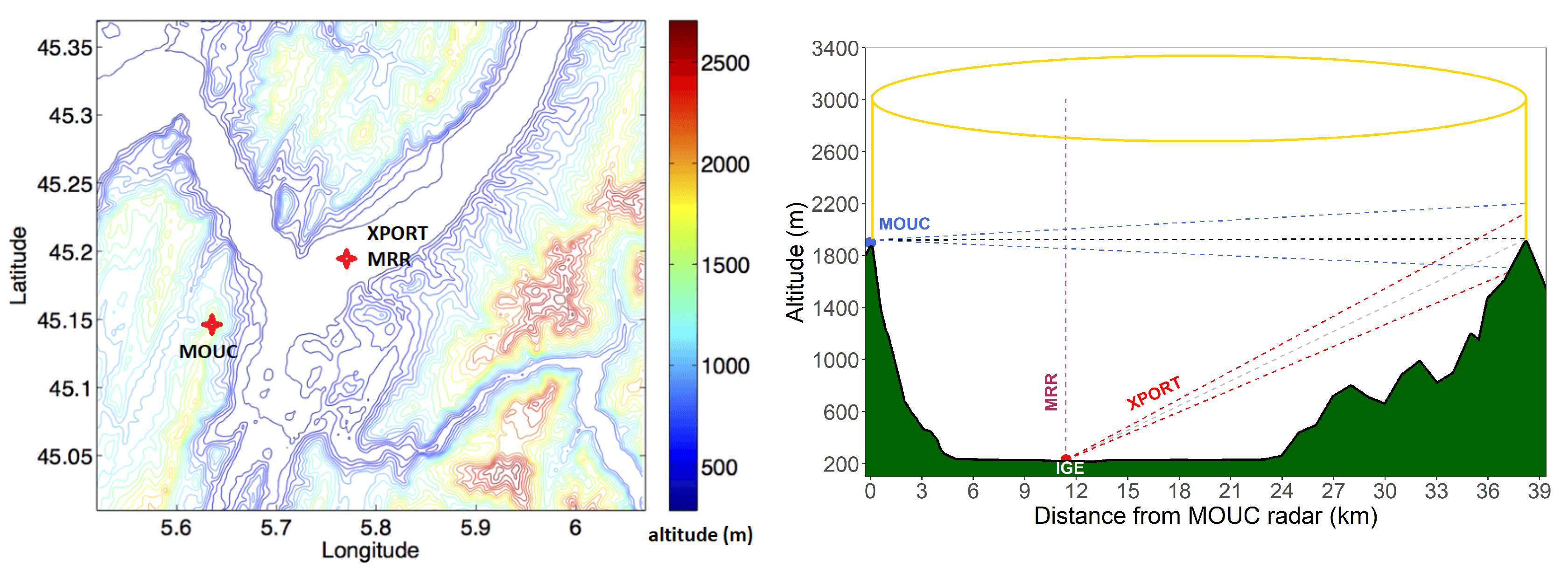
2.1. Study Site and Instruments

Grenoble is a Y-shaped alluvial valley in south-eastern France (Alps) with a mean altitude of about 220 m ASL surrounded by three mountain ranges: Chartreuse (culminating at 2083 m ASL) to the north, Belledonne (2977 m) to the south-east and Vercors (2307 m) to the west. Figure 2 shows the topography of the study area as well as the positions of the Météo-France operated radar system on top of the Mt Moucherotte (MOUC) and the IGE experimental site at the bottom of the valley.

The IGE experimental site includes the following devices:

(i)

IGE XPORT research radar [9]: X-band, dual polarized, volumetric scanning strategy,

Table 1. Characteristics of XPORT radar and numerical constants.

Symbol	Value	Unit	Parameter
$\nu$	9.4	GHz	Frequency
$P_t$	100	kW	Transmission Power
G	41.96	dB	Antenna Gain
${\theta }_{3dB}$	1.37	°	3-dB beanwidth
$\theta$	0.5	°	Angular resolution
$\tau$	1	$\mathsf{\mu }$s	Pulse width
$\Delta r$	30	m	Radial resolution
MDS	−112	dB	Minimum Detectable Signal
Numerical constants
$|K_w{|}^2$	0.93		Dielectric constant of water
$|K_i{|}^2$	0.176		Dielectric constant of solid ice
c	299,792,458	m/s	speed of light
Operating protocol	3.5°, 7.5°, 15°, 25° & 45° PPIs
Recorded parameters	$Z_h$, $Z_v$, $Z_{dr}$, ${\rho }_{HV}$, ${\mathsf{\Phi }}_{dp}$

(ii)

Micro rain radar (MRR): K-Band, FMCW [10]

(iii)

Meteorological station (MTO) including pressure, temperature, humidity, wind and rainfall intensity measurements

2.2. Datasets and Pre-Processing

The XPORT radar started recording high-resolution volumetric scan data of most significant rain events in 2016. Its operating protocol is made of 5 PPI scans at elevation angles of 3.5, 7.5, 15, 25 and 45°. It systematically records five radar parameters at radial resolution of 30 m and angular resolution of 0.5°. The recorded parameters are: horizontal reflectivity (Zh), vertical reflectivity (Zv), differential reflectivity (Zdr), cross-polar correlation coefficient (${\rho }_{HV}$) and cumulative differential phase (${\mathsf{\Phi }}_{dp}$) [11]. In this study, we consider 42 significant rain events (≥5 mm) in between November 2016 and January 2018. Due to the presence of ground clutter for the three lowest elevation angles and technical difficulties in operating the radar at 45° for a considerable period of time, we will use hereinafter only the 25° elevation angle measurements, which have a 6-min time resolution, the PPI itself lasting about 1 min. From the measurements of the recorded parameters, we produced quasi-vertical profiles (QVPs) by averaging measurements over 360° azimuth and then projecting the results to the vertical [7]. The ML identification algorithm, to be described below, performed poorly in case of large spatial variability of the 25° elevation angle measurements, notably when a rainy system was entering or leaving the valley. To limit the impact of such poor identifications on the ML statistical analyses, we used PPI scans of ${\rho }_{HV}$ to determine visually time steps with homogeneous precipitation in the various sectors of the XPORT detection domain. This sorting results in a total of 980 XPORT vertical profiles, i.e., to about 98 h of measurements. Monthly distribution of these vertical profiles is shown in

Table 2. Monthly distribution of profiles (#: number).

Month	# of Profiles	Alt Peak ${\mathit{\rho }}_{\mathbf{HV}}$
January	185	1564
February	6	1486
March	112	1303
April	119	1470
May	75	1902
September	41	2290
October	11	2715
November	224	1957
December	207	1584

. Note that the summer events are under-represented in this sample due to their convective nature, leading to strong spatial variability and subsequently poor identifications with the ML detection algorithm.

The MRR allows the continuous acquisition of the vertical profiles of Doppler Spectra of apparent fall velocities of the hydrometeors with a radial resolution of 100 m and a temporal resolution of 1 min. We applied the algorithm developed by Maahn and Kollias [12] which takes the unprocessed MRR data and apply an unfolding routine (called MK12 hereinafter) to reduce the error in Doppler spectra and fall velocity, especially in the solid phase precipitation, with respect to the original METEK algorithm. The MK12 pre-processing routine results in full Doppler spectra of apparent vertical velocities of falling hydrometeors over a velocity range of 0–12 m/s and with vertical resolution of 100 m from which we deduced the vertical profiles of the average velocity (W) and standard deviation (SW, for spectral width). Note that the MRR radar was deployed in other field campaigns in summer, so MRR data is actually available for only 27 out of 42 precipitation events being studied.

2.3. Automated Melting Layer Detection Algorithm

For its importance in micro-physical processes leading to precipitation phase change and for coping with the associated artifacts (bright band, attenuation) that affect radar QPE, the characterization of the ML has received a long-standing interest in radar meteorology [13,14] and radar hydrology [15,16] communities. Polarimetry offers unprecedented means for observing distinct ML radar signatures [14,17]: increase in reflectivity (Zh, Zv), differential reflectivity (Zdr) and differential propagation phase (${\varphi }_{dp}$), decrease in cross-correlation coefficient (${\rho }_{HV}$) within the ML. Vertical profiles of Doppler velocity spectra also bring valuable information on the hydrometeor falling velocities in stratiform precipitation [18,19]. A number of automated ML detection algorithms have been proposed to deal with radar data collected in various configurations: vertically pointing measurements [20], range-height indicators [21], PPIs at low-elevation angles [16,22], the latter being obviously the most unfavourable (small incidence angles on vertical layers, beam broadening effects) but also the common situation for QPE. In our context, we work with polarimetric QVPs [7] derived from the 25°-PPI XPORT radar measurements and with the vertical profiles of Doppler spectra derived from the MRR data. We assume attenuation and non-uniform beam filling to be of limited importance for such high-elevation angle measurements in predominantly stratiform precipitation with low intensity.

Figure 3 illustrates the working principle of the ML detection algorithm based on computation of the first and second derivatives of the QVP, a Zh QVP in that case. The “bright-band” peak corresponds to max(Zh) in the vertical profile, a first derivative equal to 0 and a minimum value of the second derivative. The bright band top and bottom correspond to the maximum values of the second derivative. The minimum of the first derivative of the reflectivity profile was found to be a distinctive figure for the reflectivity profiles: large peak value and altitude (alt2_Zh) located in between top and peak of the bright band. This altitude (alt2_Zh) is used as an initial guess for the ML position in the vertical.

Hereinafter, we denote upper and lower breakpoints of a given ML signature in QVP as “top” and “bottom” (“bot” in short), distinguishing the value and altitude coordinates of the point, e.g., Zh top altitude, Zh top value. Maxima/minima of the QVP is denoted as “peak” (e.g., Zh peak altitude, Zh peak value). For the sake of conciseness, a number of pseudo-variables are used in Tables and Figures; their description is given in Appendix A.1.

The identification algorithm for Zh works as:

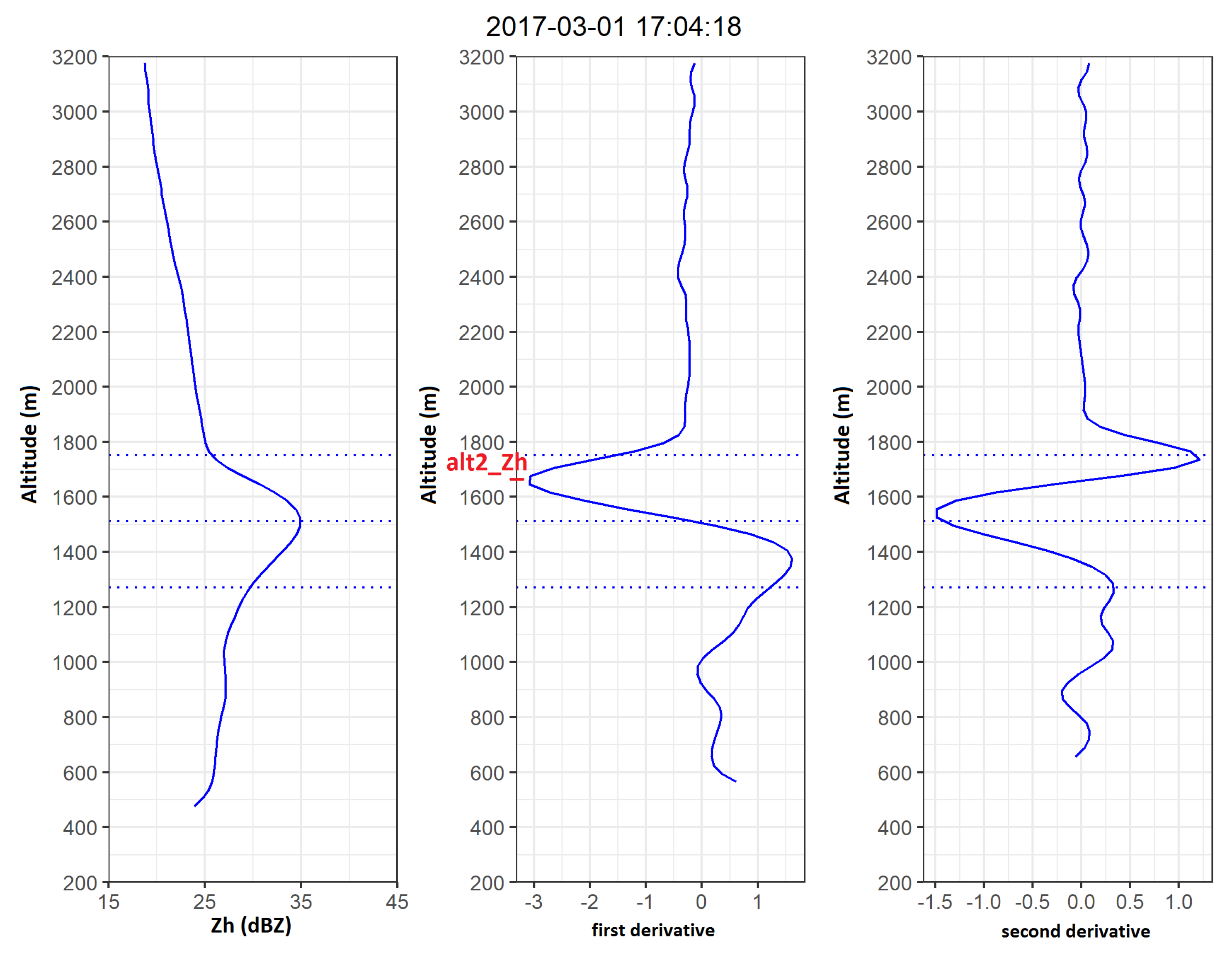
• Compute quasi-vertical profile of Zh, and its first and second derivatives.
• Find the altitude with minimum first derivative of Zh –> alt2_Zh
• Search for altitude and value of Zh peak (maxima with first derivative close to zero) up to 500 m below alt2_Zh –> Zh peak altitude and Zh peak value
• Search for Zh top altitude and Zh top value as max(second derivative of Zh) up to 300 m above alt2_Zh
• Search for Zh bot altitude and Zh bot value as max(second derivative of Zh) up to 500 m below alt2_Zh

The same algorithm works for Zv as well. Similarly for Zdr, we search for Zdr peak values and altitudes up to 800 m below alt2_Zh as max(Zdr) with first derivative close to zero. We look for top and bottom of enhancement in Zdr profile up to 500 m above and below Zdr.alt.peak, as max(second derivative of Zdr). In case of ${\rho }_{HV}$, we search for ${\rho }_{HV}$ peak up to 800 m below alt2_Zh as min(${\rho }_{HV}$) with first derivative close to zero. Then we search for ${\rho }_{HV}$ top altitude as the first altitude with ${\rho }_{HV}$ < max(${\rho }_{HV}$) − 0.02 above Zh peak. The ${\rho }_{HV}$ bot altitude is determined by symmetry. Using a single reference altitude, alt2_Zh, for identification of ML in all the radar observables (Zh, Zv, Zdr, ${\rho }_{HV}$) helps to reduce the errors in identification due to noise in different profiles in a given timestep, provided that the bright band in Zh is well observed. The time series of alt2_Zh is also used to limit the allowed jumps in reference altitudes in between two successive timesteps. Furthermore, in vertical profile of MRR derived average fall velocity (W), we look for “W top” (and “W bot”) as the maxima (and the minima) of second derivative of vertical profile of W, 500 m above and below ${\rho }_{HV}$ peak altitude.

3. Microphysics of the ML and the Vertical Profiles of Radar Observables

In this section, we aim to perform a detailed analysis of ML with the help of QVPs of Zh, Zv, Zdr, ${\rho }_{HV}$ and vertical profile of W, their relationship with each other, definition of melting layer boundaries and associated micro-physical processes. The QVPs of ${\varphi }_{dp}$ are not considered in this article since they were found to be too noisy and hardly exploitable for a large majority of the considered events, as they have generally low precipitation intensities. The analysis of a single timestep (e.g., 1 March 2017 17:04:18 in Figure 4) provides detailed insights into the vertical structure of rainfall and micro-physical processes associated with the melting layer, especially the hydrometeors’ evolution with time and/or height. A stratiform rain event with 9 mm of cumulative rainfall spread over 11 h window is discussed here. At the given timestep, rainfall intensity and temperature at MTO station were $2\mathrm{mm}\mathrm{h}{}^{-1}$ and 7.8 °C respectively. Top of the brightband can be observed at 1770 m ASL, a bit below the 0 °C isotherm at 1790 m estimated by the Météo-France AROME NWP model. The quasi vertical profiles of polarimetric and vertical profiles of Doppler observations from XPORT (left) and MRR (right) radars are displayed in Figure 4. Vertical profiles of XPORT are normalized between [0–1] to show the vertical profiles of Zh, Zdr and ${\rho }_{HV}$ in a single plot.

$$\begin{gathered} \mathrm{Zh},\mathrm{Zv}:[15,45]\mathrm{dBZ}-->[0,1] \\ \mathrm{Zdr}:[-3,3]\mathrm{dB}-->[0,1] \\ {\rho }_{HV}:[-0.65,1]-->[0,1] \end{gathered}$$

As falling ice particles move from $-5°$ to $0°\mathrm{C}$, they grow by aggregation, resulting in larger particles and in a reduction in the number of smaller particles [23], this might be an explanation for the gradual decrease in reflectivity above the ML in Figure 3 (left). When they pass through the $0°\mathrm{C}$ isotherm, they receive latent heat of fusion from the atmosphere. Ice particles start to melt and become wet. The latent heat required cools the air, leading to a quasi-0 °C temperature layer. They continue to descend, encounter warmer air and melt completely, eventually collapsing to rain drops much smaller than original icy hydrometeors of same mass and higher fall velocities.

Textbooks [24] and articles based on in-situ observations [25,26,27], wind-tunnelling experiments [28] and modelling studies [29,30] on snowflake melting processes establish that the melting of individual hydrometeor (or an aggregate) occurs in several stages in an atmospheric column, that we may summarize as follows:

• In the first stage, melting starts at the tips of ice branches on the entire periphery, but mainly at the bottom of the snowflake.
• In the second stage, aerodynamic drag helps the meltwater to flow and surface tension draws meltwater preferentially into concave regions, e.g., from periphery to the linkages of the snow crystals comprising of aggregates, minimizing the capillary forces and surface tension effects. The hydrometeor is not covered by meltwater in this stage, as the main ice-frame is still intact and the icy hydrometeor has ragged surface.
• As these enclaves fill up and the edges erode due to melting, in the third stage, liquid water flows out of the filled concave regions, merges with other nearby liquid bodies, and melt water seeps into branches inside the snowflakes breaking the ice lattices. Surface tension stabilizes the hydrometeor into new equilibrium shapes and consequently the crystal mesh changes from one with many small and sharp protrusions to one with a few smoother and larger protrusions.
• Towards the end of melting process, in the fourth stage, the weak connections of ice separating drops/liquid water bodies become sufficiently thin to fracture under aerodynamic forces or simply melt away relatively quickly. The particle assumes a spherical shape, initially around an ice core and eventually forming a water drop. Through the melting process, hydrometeors undergo change in shape and ice/water content leading to smaller particles with higher mass density, which results in increase of fall velocities as they also experience less air resistance.

Melting of a distribution of hydrometeors in a stratiform rainfall produces distinct signatures of radar observables on ground-based Doppler and polarimetric radars (Figure 4). Zh and Zv are sensitive to the phase (liquid, solid), concentration and size distribution of hydrometeors. Zdr is a proxy for their shape anisotropy and variation of particle orientation. ${\rho }_{HV}$ is a measure of coherence of the observations made in the horizontal and vertical polarisations, and as such, a good indicator of precipitation homogeneity within the resolution volume.

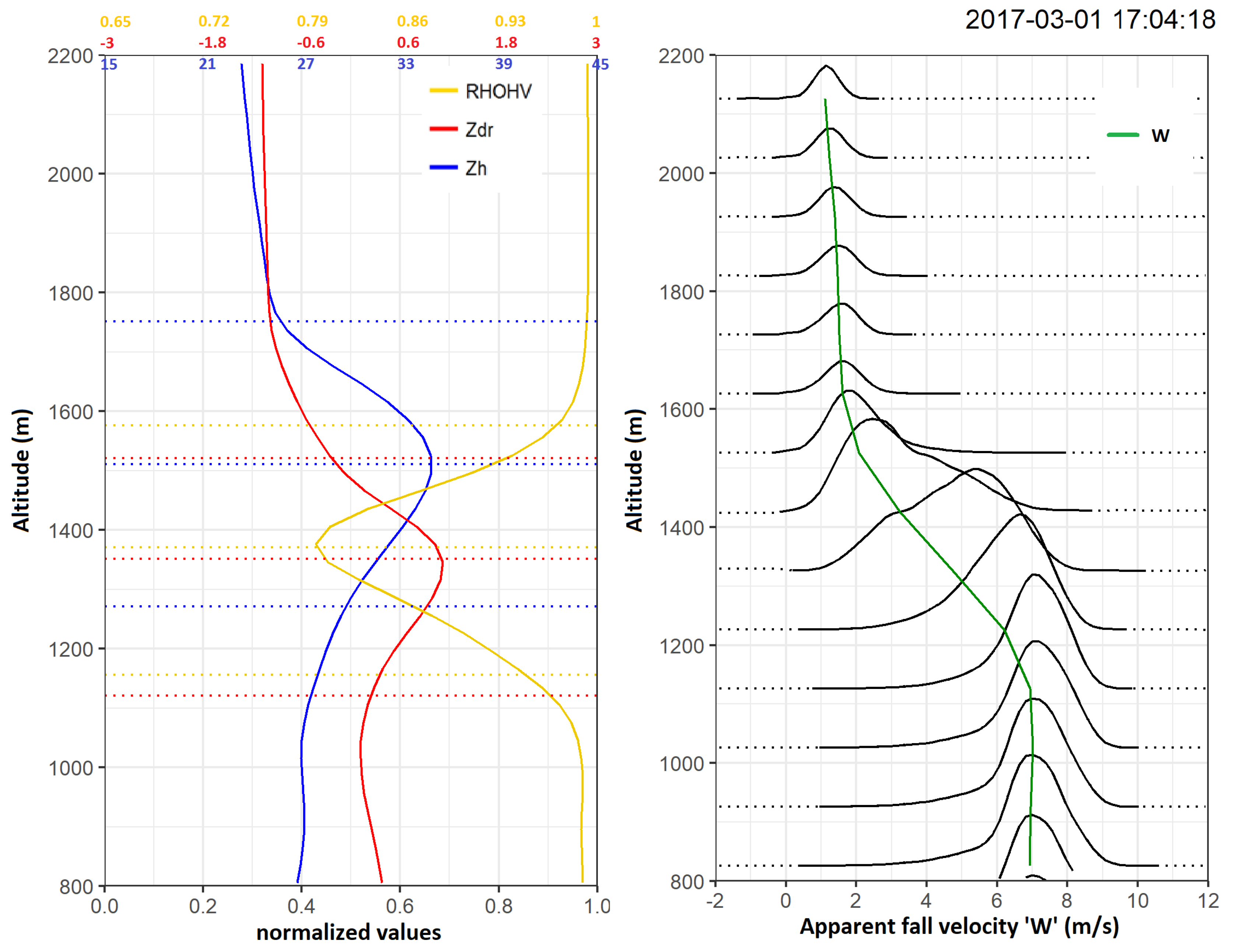
• With aggregation as the dominant process, from 1000 m above the ML, there is an increase in radar reflectivity (Zh, Zv) of 6 to 7 dBZ, as observed in Figure 3 and Figure 4, with little dependence on precipitation intensity, consistent with [14]. Small snowflakes melt faster than the big ones, causing some particles to fall faster than others and thus increasing probability of aggregation and coalescence. In an atmospheric column with steady precipitation, assuming stationarity, this leads to an increase in the particle size (in case of aggregation) or an increase in number density (if no aggregation) at a layer lower than the initial level. This leads to steady increase in Zh below initial 0 °C isotherm. When most big particles are at end of 3rd stage of melting, i.e., with thin shell of meltwater with ice-core, they essentially have size of the ice-particle and di-electric constant of water. These few large highly reflective particles, resembling big raindrops to a radar, explain the maximum of the reflectivity profile; around 10 dBZ bigger than the value at ML top for the example of Figure 3 and Figure 4. The bright band peak is said to occur at a level where the particles have attained the high scattering property of water drops but have not yet attained their velocity [31]. As these big particles start to melt and gain higher falling velocities, the number concentration at the given altitude of the atmospheric column decreases. This causes a gradual decrease in reflectivity in the lower portion of ML (below thw altitude of Zh peak); reflectivity remains more or less constant below the ML.
• Differential reflectivity (Zdr) is positive for particles whose major axes aligns close to horizontal, zero for spherical particles/particles with random distribution of orientation, and negative for vertically oriented particles. Big rain drops tend to flatten and orient themselves with major axes close to horizontal. Pristine ice crystals have small axis ratio (horizontal to vertical) and high bulk density, and fall with their major axes close to horizontal i.e., high Zdr. Aggregates have large axis ratio, low bulk density and low dielectric constant resulting in “effectively isotropic” shape, so low Zdr(∼0.5 dBZ) [17,32]. The vertical profile of Zdr is slightly different from Zh. Zdr increases as well during melting, but the maximum develops at lower altitude than Zh. A peak with positive value of Zdr below Zh peak indicates an oblate mean shape at that height, and the small values above and upper part of ML indicates isotropic mean shape while individual ice particles can be very irregular [29]. As the particles smoothen due to faster melting of protrusions, Zdr decreases on the upper part of melting layer, and just before the ice-structure crumbles in 4th stage of melting Zdr peaks rapidly, to 1 dB during this event. This suggest maximum anisotropy of hydrometeors occurs at lower altitude than maximum size. Surface tension during 4th stage of melting (following collaspe of ice-structure) acts much quicker compared to other melting processes. As hydrometeors assume more spherical shape, Zdr decreases quickly i.e., the vertical profile of Zdr enhancement is non-symmetric. This decrease in Zdr might also be a result of break-up of large melted aggregates [33]. Rain drops take more oblate shape, as they reach terminal velocity. It is noteworthy to remind that the elevation angle of 25° is used in this study, Zdr measurements within the ML might be more pronounced at lower scanning angle.
• Co-polar cross correlation coefficient (${\rho }_{HV}$) is sensitive to changes in shape, size, orientation and thermodynamic phase of hydrometeors between successive pulses. It might be sensitive to elevation angles of PPI scan in mixed-phased regions [34]. Vertical profile of ${\rho }_{HV}$ shows relatively high values (∼0.99) above (in snow) and below (in rain) the ML with a sharp decrease in the lower part of ML. Some ML detection algorithms (like [22]) use ${\rho }_{HV}$ < 0.97 as a threshold criterion for mixed phase of precipitation. Decorrelation occurs if the two orthogonal backscattered waves do not vary in unison, i.e., with the change in net effective backscattering properties at horizontal and vertical polarization in the resolution volume. The decrease in correlation is pronounced for wet, large and irregular hydrometeors [35], likely a consequence of a greater variety of shapes and axis ratios associated with partly melted particles and introduction of raindrops [17]. ${\rho }_{HV}$ minima occurs below the Zh maxima and slightly above the Zdr maxima (Figure 4), where some large particles are asymmetric with ice-frame still intact while some have already crumbled under surface tension to become more spherical.
• Vertically pointing MRR provides vertical profile of hydrometeor’s apparent fall velocity spectra(S(v)). The Doppler spectrum $S\left(v\right)$ is the power-weighted distribution of radial velocities within the resolution volume, i.e., $S\left(v\right)$ represents the power returned to the radar by scatterers with radial velocity between v and $v+\Delta v$. The average radial velocity (W) is the first moment of the normalized Doppler spectrum, and spectral width is the square root of normalized second moment. Spectral width is a measure of dispersion of velocities within the resolution volume. Unlike other radar observables, average fall velocity has a monotonously decreasing vertical profile (with increase in elevation) within the ML. Above ML, snow has average fall velocity of 1–2 m/s; presence of crystalline ice, super cooled water and air updrafts/downdrafts can affect the average fall velocity of snow. Towards the end of 3rd stage of melting, hydrometeors smoothen causing decrease in aerodynamic drag and slight increase in fall velocity. During the 4th stage of melting, as hydrometeor melt fraction increases, its density increases and it assumes more spherical shape (size decreases), which also aids to decrease aerodynamic drag and to increase fall velocity. As the largest hydrometeors melt completely and become spherical rain drops, the average fall velocity reaches a maximum. As the raindrops continue to fall, they might assume oblate shape resulting in a slight decrease of the fall velocity to reach the terminal velocity of 6–8 m/s. At low rainfall intensities raindrops are small and remain mostly spherical and this decrease might be negligible, like in Figure 4. Some ML detection algorithms (like [36]) use the altitude of maximum average velocity as the bottom of ML. At the altitude of Zh peak, the average fall velocity is still close to fall velocity of snow. The Doppler velocity spectra is very narrow above and below ML, centered at terminal velocity of snow and rain respectively. Within the melting layer, the spectral width broadens gradually with decrease in ${\rho }_{HV}$, reaches maximum value at altitude with minimum ${\rho }_{HV}$, and it contracts again with increase of ${\rho }_{HV}$.

4. Statistical Analysis of the ML Characteristics

Here, we study the climatology of the melting layer based on the available dataset of 42 rain events. We will seek to understand the dependence of ML parameters on altitude of the $0°\mathrm{C}$ isotherm, intensity of rainfall at ground and density of snow. Being a standard hypothesis of 1D ML models [16], 1 to 1 correspondence of snowflake to raindrop is a question of interest. The added value of Doppler and polarimetric measurements with respect to reflectivity measurements for the analysis of melting layer is also a subject of interest in this study.

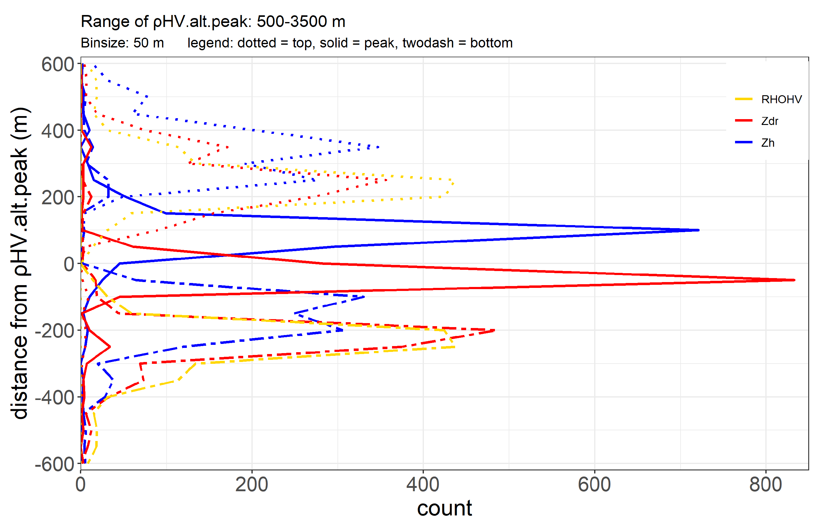
4.1. ML Boundaries and Vertical Organization of the ML

Let us first consider the altitudinal dimension of ML characteristic points. Our experience with the ML detection algorithm indicates that ${\rho }_{HV}$ peak is the most consistently identified signature, and we expect it to be in between altitudes of Zh peak and Zdr peak. Figure 5 shows the probability distribution functions (pdf) of different distances between radar signatures, i.e., top, peak and bottom of Zh, Zdr and ${\rho }_{HV}$, with respect to the ${\rho }_{HV}$ peak altitude, computed over the entire dataset of 980 profiles; a number of statistics (mean, standard deviation and quantiles of these distributions) are listed in

Table 3. Statistics of ML altitudes in terms of mean, standard deviation and quantiles. (see Appendix A.1 for the definitions of pseudo-variables).

	Units	Mean	Std.Dev	Q10	Q25	Q50	Q75	Q90
Zh.alt.top	(m)	2041	450	1411	1621	2071	2311	2671
Zh.alt.t2p	(m)	265	80	180	210	240	300	360
Zh.alt.p2b	(m)	268	81	180	210	240	300	360
Zdr.alt.t2p	(m)	274	87	180	210	270	330	390
Zdr.alt.p2b	(m)	208	57	150	180	180	240	270
${\rho }_{HV}$.alt.t2p	(m)	254	76	180	210	240	270	330
${\rho }_{HV}$.alt.p2b	(m)	254	76	180	210	240	270	330
Zh.alt.peak − ${\rho }_{HV}$.alt.peak	(m)	90.21	66.06	30	60	90	120	150
${\rho }_{HV}$.alt.peak − Zdr.alt.peak	(m)	30	48	0	30	30	30	60
ML width	(m)	609	162	450	510	600	690	780

.

We note that the pdfs of Zh and Zdr peak altitudes are quite narrow. The mean distance between ${\rho }_{HV}$ peak and Zdr peak is around 30 m, while the average distance between ${\rho }_{HV}$ peak and Zh peak is around 90 m. The distributions of the altitudes of the top and bottom are flatter compared to that of the peaks. The vertical profile of ${\rho }_{HV}$ in ML is symmetric, by construction, with top and bottom at 225 m from the peak value. Zh top and ${\rho }_{HV}$ bottom are the altitudes furthest from ${\rho }_{HV}$ peak. Study of ML microphysics in Section 3 shows that Zh is the first radar observation to change significantly when the particles are still in early stages of melting. So like Fabry and Zawadzki [14] we assume that Zh top coincides with 0 °C isotherm. We also observe that ${\rho }_{HV}$ bottom and max(W) occur at similar altitudes in Figure 4, both of which signify the end of melting process. So, in this study we will refer Zh.alt.top as ML top and ${\rho }_{HV}$.alt.bot as ML bottom. Hence, ML width = Zh.alt.top − ${\rho }_{HV}$.alt.bot. In our observation (Table 3), the mean ML width is 609 m; Q10 and Q90 of ML width are 450 m and 780 m respectively.

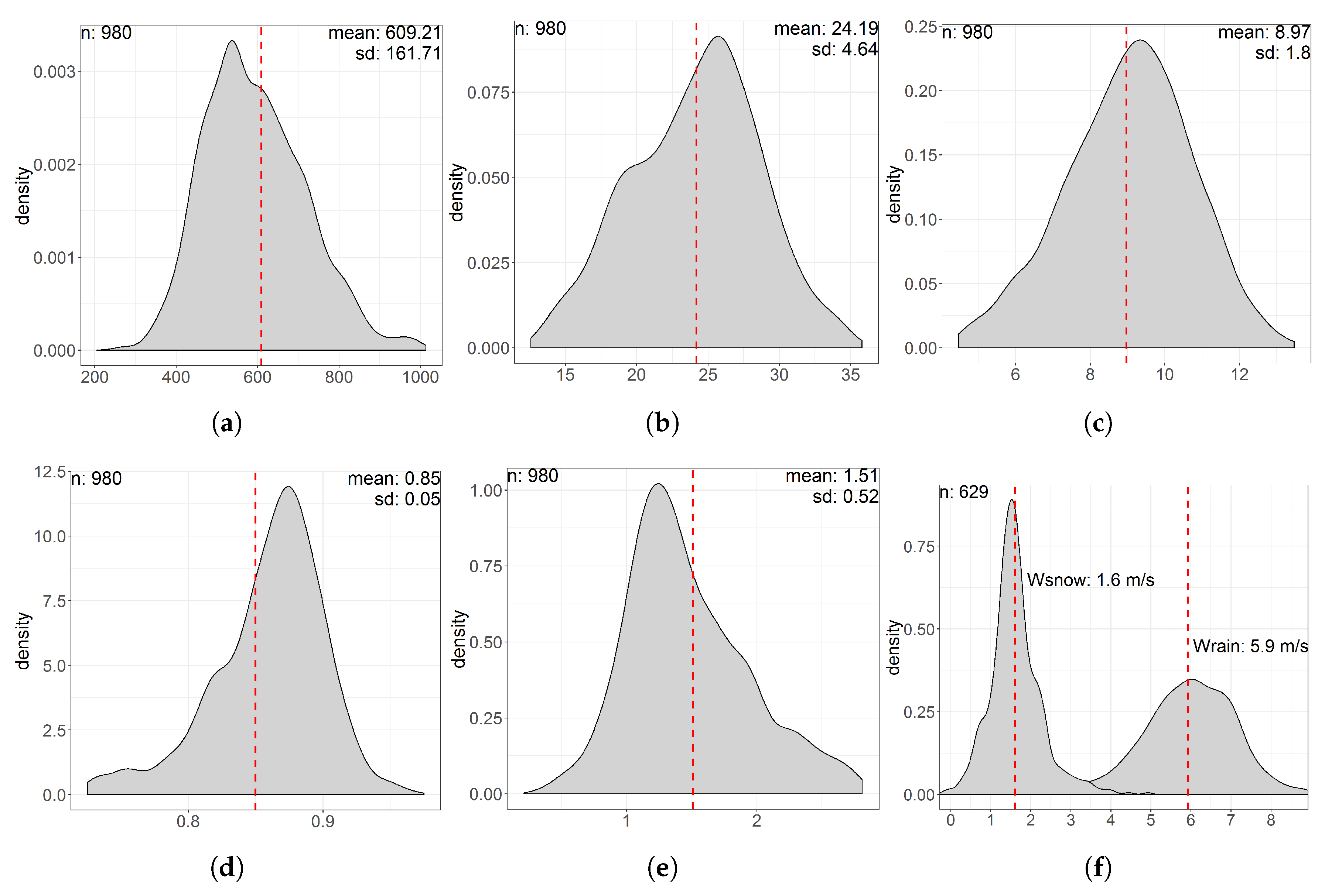
4.2. Statistics of ML Characteristic Values

Table 4. Statistics of ML characteristic values. (see Appendix A.1 for the definitions of pseudo-variables).

	Units	Mean	Std.Dev	Q10	Q25	Q50	Q75	Q90
Zh.val.bot	(dBZ)	24.19	4.64	18.07	20.85	24.59	27.38	29.89
Zh.val.t2p	(dBZ)	8.97	1.80	6.70	7.87	9.13	10.19	11.15
Zh.val.p2b	(dBZ)	6.37	1.69	4.14	5.49	6.56	7.38	8.13
Zdr.val.peak	(dB)	0.63	0.61	−0.08	0.2	0.57	0.99	1.49
Zdr.val.t2p	(dB)	1.24	0.41	0.82	0.99	1.18	1.4	1.8
Zdr.val.p2b	(dB)	1.51	0.52	0.96	1.15	1.4	1.8	2.25
${\rho }_{HV}$.val.peak	(-)	0.85	0.05	0.79	0.83	0.87	0.89	0.9
Rainrate	(mm/h)	1.45	1.04	0.48	0.72	1.24	1.85	2.66
Wsnow	(m/s)	1.6	0.75	0.85	1.28	1.56	1.91	2.37
Wrain	(m/s)	5.92	1.2	4.46	5.24	6.01	6.73	7.23

presents the statistics of the reflectivity and polarimetric values and Figure 6 displays normalized pdfs of some of these variables. As a first guess, we considered the Marshal-Palmer relationship ($R={(Zhbot/200)}^{1/1.6}$ with Zh bot in ${\mathrm{mm}}^6{\mathrm{m}}^{-3}$) as an estimate of rain rate (R in $\mathrm{mm}{\mathrm{h}}^{-1}$) below the ML. Wsnow and Wrain are hydrometeors’ apparent mean fall velocity in snow (60 m above ML top) and rain (100 m below ML bottom) respectively.

Table 4 shows that the events considered in this study have a rather limited range of rain rate values, 0.48 $\mathrm{mm}{\mathrm{h}}^{-1}$ at 10% quantile, 2.66 $\mathrm{mm}{\mathrm{h}}^{-1}$ at 90% quantile and a maxima of 8.47 $\mathrm{mm}{\mathrm{h}}^{-1}$. This is mostly due to the difficulties in identifying ML during convective events, often associated with high rainfall rates, as they have high horizontal variability. Figure 6 shows that the variables of interest are generally monomodal with limited skewness. This is why various pdf quantiles are listed in Table 4. Both the altitude and value statistics (Table 3 and Table 4) are in overall agreement with similar X-band radar observations [21] of ML made at Davos and Ardeche, except the mean ML width which is wider in our observations, possibily a result of different estimation mode between two studies.

The correlation matrix of the ML descriptors is shown in Figure 7. Due to the limited skewness of their individual distributions and the likely non-linear relationships between pairs of them, we have computed the Spearman’s rank correlation coefficient, more relevant for monotonic non-linear relationships than the classical Pearson’s linear correlation coefficient. Zh top, Zh bot, Zh peak and R show high correlation with each other. The correlation coefficient of 1 between Z bot and R results simply from the power-law transformation (deterministic and monotonic) applied. This high level of correlation is to be expected as the size and concentration of icy hydrometeors above ML are the common factors controlling these variables. Interestingly, the ${\rho }_{HV}$ peak value correlates also significantly with Zh top, Zh bot, Zh peak and R. We note that it correlates more with Zh peak than with Zh top or Zh bot. This confirms that Zh peak is more sensitive to presence of large particles than to the number concentration. In addition, we note that the Zdr peak value is significantly correlated with ${\rho }_{HV}$ peak value (which is also sensitive to particle orientation) and to a lesser extent to the reflectivity and rainrate descriptors. ML width correlates more with the reflectivity variables than with the polarimetric ones. Wsnow is essentially uncorrelated to all the other variables while Wrain is more correlated with the reflectivity and rainrate variables than with the polarimetric ones.

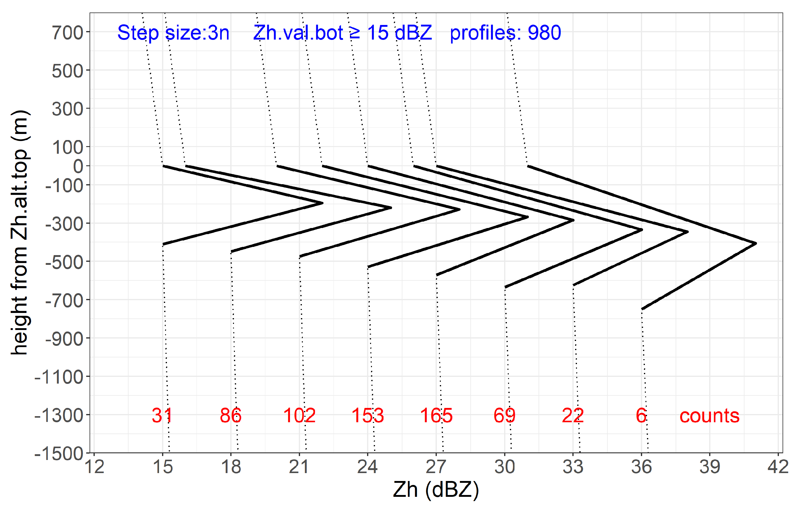
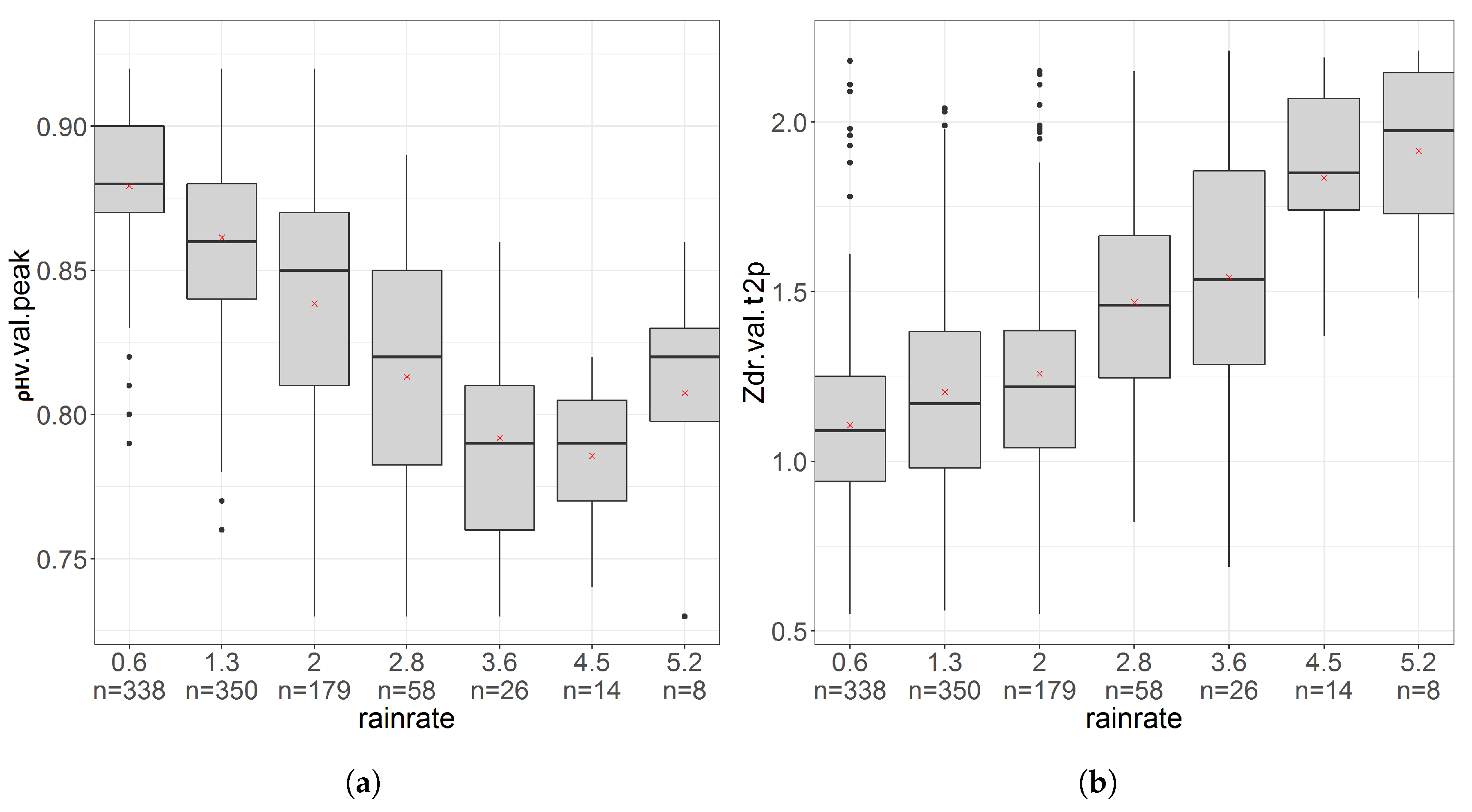
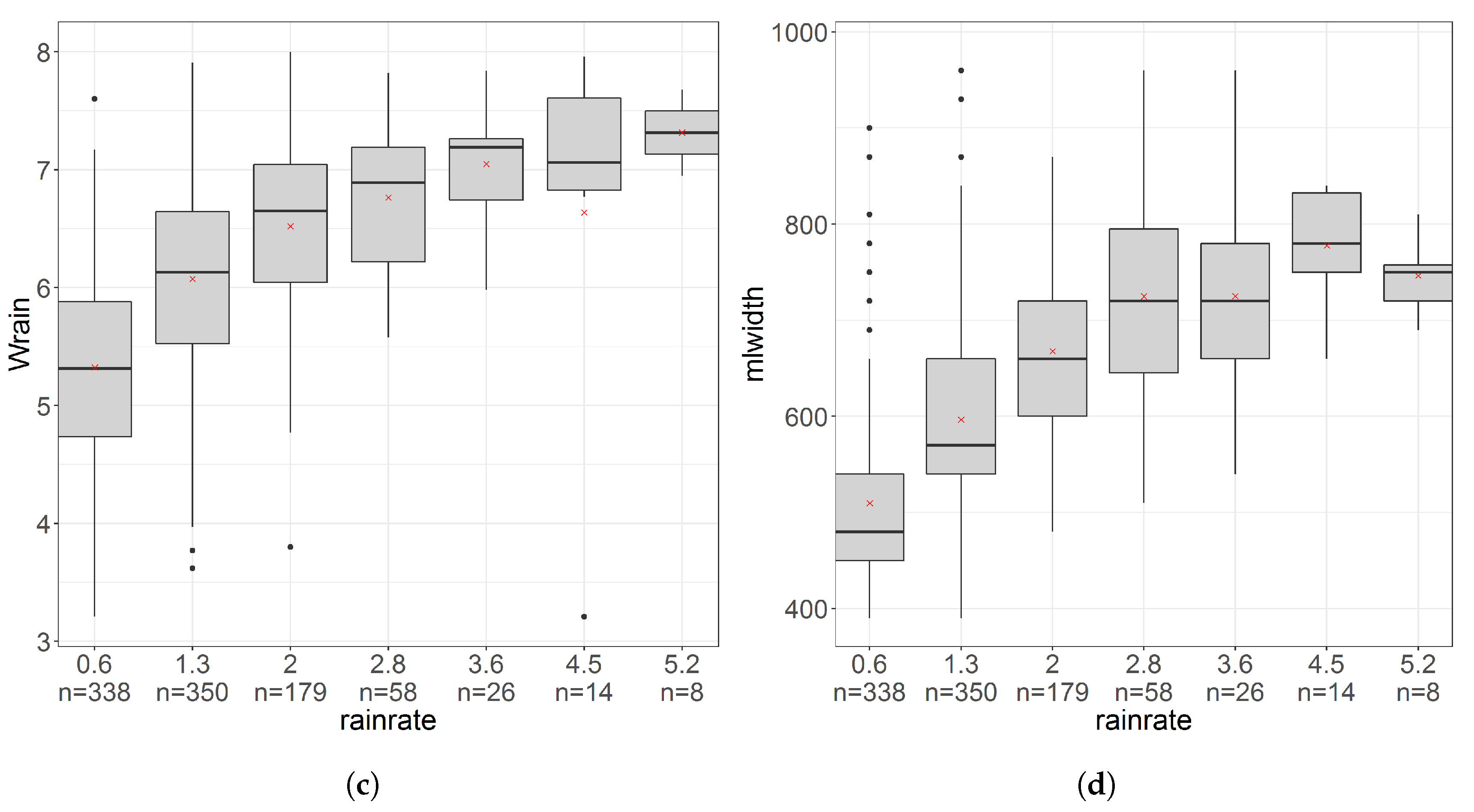
4.3. Evolution of ML Descriptors with Rainfall Intensity

During the events under study, rainfall in Grenoble valley has a slightly right skewed distribution with mean at 1.45 $\mathrm{mm}{\mathrm{h}}^{-1}$ and standard deviation of 1.04 $\mathrm{mm}{\mathrm{h}}^{-1}$. As noted previously Zh top, Zh bot and Zh peak show high correlation with each other. Inspired by Figure 10 of [14] we examine the relationships between Zh bot and three descriptors of the reflectivity profile: Bright Band (BB) width (altitude difference between Zh top and Zh bot), Zh top and Zh peak in Figure 8. As observed in [14] the BB width increases slowly till the Zh bot of 21 dBZ, beyond which the increase is rapid. Till 21 dBZ (

Table 5. Summary: Intensity effect.

Zh val.top	Zh val.t2p	Zh val.p2b	BB width	Zh alt.t2p	Zh alt.p2b
(dBZ)	(dBZ)	(dBZ)	(m)	(m)	(m)
15	7	7	410	194	216
18	9	7	448	219	229
21	8	7	474	228	246
24	9	7	528	267	261
27	9	6	570	284	286
30	10	6	634	334	300
33	11	5	623	345	278
36	10	5	750	405	345

), Zh.alt.p2b is bigger than Zh.alt.t2p, after which the former increases faster than the latter. Our explanation is as follows: at higher rainfall intensities there is higher probability of irregular shapes and aggregation above ML, resulting in particles with big concavities. When the ice particles start to melt, it takes longer to fill these concavities before a thin shell of liquid water can form around the biggest particles (Zh peak), followed by longer melting period (stage 4) for larger particles.

Another observation in Figure 8 and Table 5 is the increase in Zh.val.t2p and decrease in Zh.val.p2b with increase in reflectivity below the ML. It can be attributed to increase in particle size with increase in rainfall; another possible contribution is from microwave attenuation at higher rainfall intensities as raw data is used in this study i.e., without attenuation correction. Most models for vertical profiles of equivalent reflectivity (using ${\left|Kw\right|}^2$ from Table 1 for whole profile), assume that one snow particle results in one rain drop; this assumption seems to be refuted above 21 dBZ as well.

As further illustrations of the correlation matrix results in Figure 7 for polarimetric and Doppler variables, the evolution of ${\rho }_{HV}$ peak value, the differential reflectivity enhancement on top of the profile (Zdr.val.t2p) and the Doppler mean velocity in rain (Wrain) as a function of R is displayed in Figure 9. The evolution of the ML width, a priori slightly different from the BB width, is displayed as well as a function of R. Rainrates are divided into 7 classes, and mean intensities of each class are the X-labels. In each class, the distribution of the considered variable is presented in the form of box plots. As expected, the relationships are essentially non-linear. We underline that the upper two rainrate classes have low number of values, thus diminishing the significance of the trends observed there. Let us recall that with increase in intensity we expect increase in concentration, size, coalescence and increased diversity in shape/orientation of icy hydrometeors above the ML. With increase in number concentration and size of hydrometeors, we expect wider ML (Figure 9d) as more latent heat is required to melt large number of ice particles. Bigger particles size also means higher fall velocity (Figure 9c) and longer melting time, both of which resulting in the ML widening. Terminal velocity of rain drops depends on size, shape and mass of raindrops, and the density of air. At low rain intensity (drizzle), particles are smaller, resulting in lower terminal velocity. Correlation matrix [Figure 7] as well shows considerably high correlation of both fall velocity and ML width with rainrate. With increase in diversity of shape, size and orientation of icy hydrometeors, we expect increase in Zdr.val.t2p within ML with increase in rainfall intensity. In Figure 9b we can observe that the Zdr enhancement almost doubles (from 1.1 dB to 1.9 dB) as rainfall intensity increases from 0.6 to 5.2 $\mathrm{mm}{\mathrm{h}}^{-1}$. Finally, increase in diversity in shape, size, orientation, fall speed of melting particles within the pulse volume results in significant decrease of ${\rho }_{HV}$ peak value as rainrate increases (Figure 9a). At low rain intensity, ${\rho }_{HV}$ peak value is quite high around 0.88 for rain-rate of 0.6 $\mathrm{mm}{\mathrm{h}}^{-1}$; it drops to 0.78 around rainfall intensity of 4.5 $\mathrm{mm}{\mathrm{h}}^{-1}$. A larger dataset would be necessary to determine if the non-monotonic trends visible for ${\rho }_{HV}$ peak value and ML width for the highest rainrates are significant.

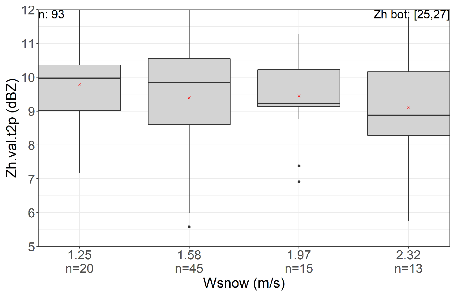
4.4. Evolution of ML Characteristic Values as a Function of Rainrate and Altitude of the 0 °C Isotherm

In this sub-sections, we detail the correlation structure of the ML descriptors as a function of the rainrate, considered as the most natural variable for describing the intensity of the phenomenon of interest (precipitation), and the ML top altitude, as a proxy for the 0 °C isotherm altitude.

Selection of physical explanatory variables helps to associate different ML radar signatures to different physical processes occurring in the ML. 0 °C altitude and rainfall intensity at ground are the two most trivial and easy to investigate explanatory variables. Temperature profile is another possible explanatory variable for rates of melting process, most probably associated with width of ${\rho }_{HV}$ decrease and vertical distance between Zh peak value and ${\rho }_{HV}$ peak value. Hydrometeors types (distribution and shape) are related to Zdr peak value and ${\rho }_{HV}$ peak value. Hydrometeor density can be another explanatory variable associated with Wsnow and the reflectivity enhancement on top of the profile (Zh.val.t2p). In this sub-section, we limit ourselves to study the relationship of some of the ML descriptors with the rainrate and the 0 °C isotherm altitude, using R and ML top derived from the radar dataset available as proxies. Investigations of other explanatory variables could be possible and desirable, e.g., with high-resolution NWP model outputs; this will be the subject of future research.

Using partial correlation coefficients in Figure 7, we computed the total correlation coefficients $r_{1.23}$ (Appendix A.2) of different ML characteristic values as explained variables (index 1) as a function of the two explanatory variables (ML top and R). The most interesting results are displayed in

Table 6. Spearman’s multiple regression with two explanatory variables: var 1 is the variable of interest, var2 and var3 are explanatory variables, ML top and R, respectively. ’r’ is the Spearman’s correlation coefficient between variables represented by subscripts.

var1	var2	var3	r12	r13	r23	r1.23
Zh.val.t2p	ML top	R	0.13	0.52	0.18	0.52
${\rho }_{HV}$ peak	ML top	R	0.16	−0.58	0.18	0.64
Zdr.val.p2b	ML top	R	−0.28	0.57	0.18	0.69
Zh.alt.peak − ${\rho }_{HV}.alt.peak$	ML top	R	−0.24	0.43	0.18	0.54

. First we note that ML top is poorly correlated with R in correlation matrix Figure 7 ($r_{23}$ = 0.18). This is desirable, as the addition of second explanatory variable promises new information, potentially adding value in the explanation of variable of interest with respect to the first explanatory variable. The added value can be quantified by comparing the total correlation coefficient $r_{1.23}$ with the absolute value of highest partial correlation coefficient $r_{12}$ or $r_{13}$. We found that there is actually little or no added-value with the second variable most of the time, e.g., for Zh.val.t2p in Table 6, but also for Zh top value, Wsnow and Wrain. However, there is a significant improvement on ${\rho }_{HV}$ and Zdr observations, i.e., +6 points improvement in explanation of ${\rho }_{HV}$ peak and +12 points improvement in explanation of Zdr enhancement at the bottom of the profile (Zdr.val.p2b), +11 points improvement in explanation of the altitude difference between the ${\rho }_{HV}$ peak and the Zdr peak values. As visible in Table 6 and equation in Appendix A.2, such gains in correlation are significant when $r_{12}$ and $r_{13}$ are of opposite sign, $r_{23}$ being positive. The physical interpretation of such statistics is not trivial, but they do draw our attention towards the complex interplay of melting processes on polarimetric radar observables.

4.5. Density Effect on Bright Band

The study [19] suggests that, for comparable precipitation rates, snow density affects the brightband intensity i.e., high density hydrometeors result in lower reflectivity peak due higher falling velocities and smaller particle sizes. Faster falling hydrometeors lead to lower number concentration which results in decrease of reflectivity. Larger icy hydrometeors, when covered with thin layer of water towards the end of second stage of melting (Section 3), appear as large particles with high dielectric constant to a radar, effectively produces strong reflectivity signature. Conversely, smaller particles lead to smaller reflectivity peak. The co-existence of supercooled cloud water with snow above ML, leading to riming and change in snow densities. For stratiform precipitation with a melting layer, the authors propose high density hydrometeors above ML can result in smaller BB enhancement. Faster falling hydrometeors lead to lower number concentration and a decrease in reflectivity.

In order to check if this effect is visible in our dataset, in Figure 10 we examine the effect of snow density on BB enhancement. As most of the events under study are stratiform events with max rainfall intensity of 8.47 $\mathrm{mm}{\mathrm{h}}^{-1}$, we do not have significant number of observations at the last interval i.e., mean(Wsnow) > 2.3 $\mathrm{m}{\mathrm{s}}^{-1}$ as seen in Figure 10. For a small class of reflectivity values below ML, [25–27 dBZ], we observe a decrease in BB enhancement of 1 dBZ with the increase in snow velocity/density.

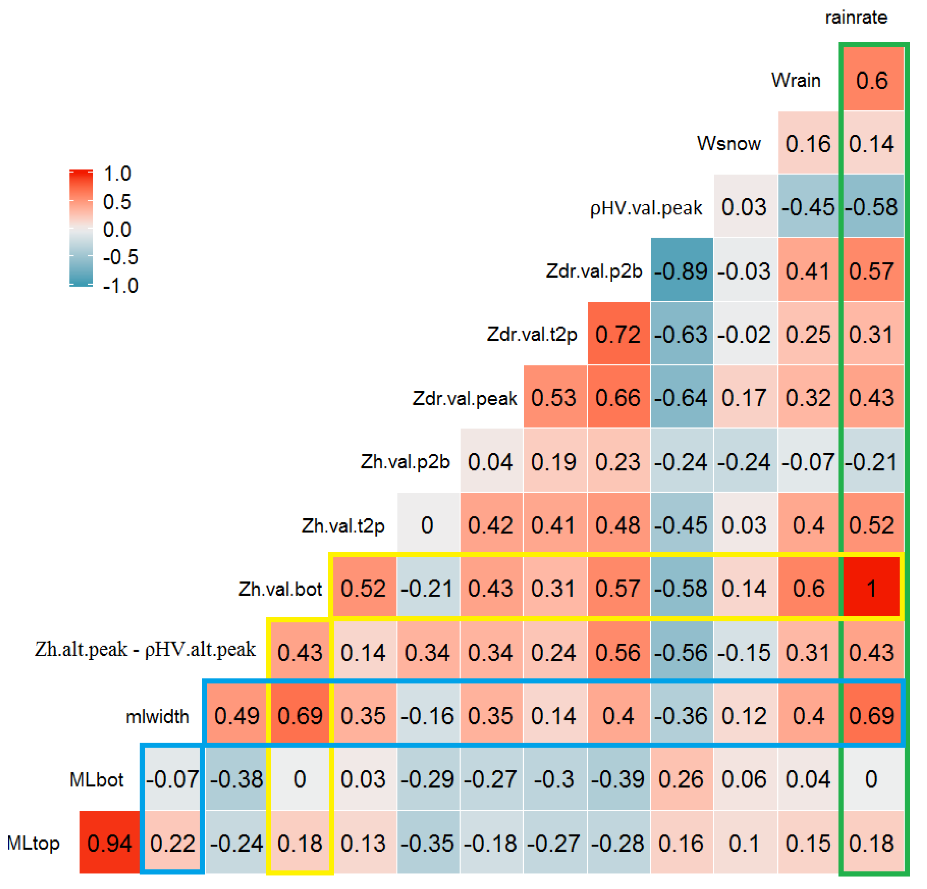
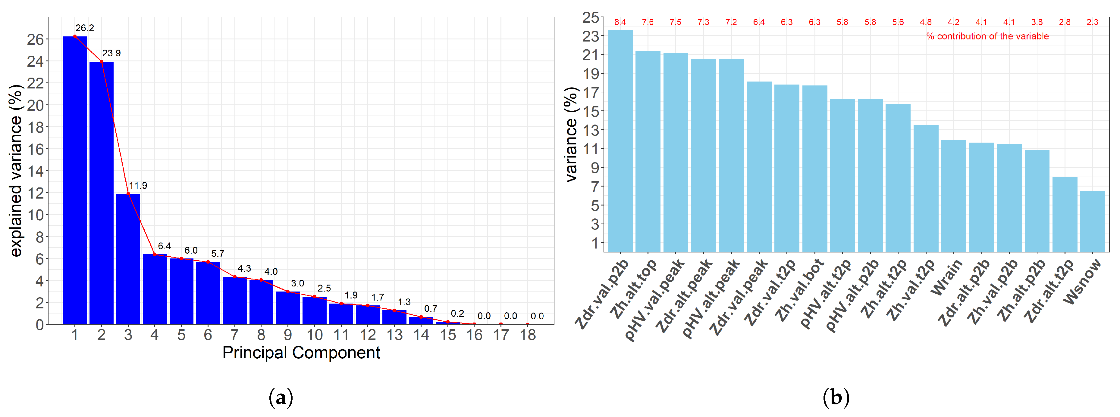
4.6. Information Content of the ML Dataset

In order to investigate more deeply the information content of the ML dataset available, we have implemented a number of statistical techniques ranging from Principal Component Analysis (PCA) to more complex clustering techniques, e.g., Kohonen’s self-organizing maps. In this article we simply present results from the PCA technique. We remind that PCA is a statistical procedure that uses an orthogonal transformation to convert a set of observations of possibly correlated variables into a set of values of linearly uncorrelated variables called principal components (PCs). By ordering the principal components, it is possible to reduce the dimensionality of the dataset if first few PCs retain most of the variance present in all of the original dataset. Here, we have selected 18 variables (x-labels of Figure 11b), assumed to be representative of the total variance present in vertical profiles of Zh, Zdr, ${\rho }_{HV}$ and W within the ML. Figure 11a shows that the first two PCs only explain about 50% of the total variance and that we need at least 9 PCs to explain 90% of the dataset variance. Lack of dominance of a few PCs is an indication that the dataset is quite rich and that polarimetric and Doppler variables bring significant information with respect to reflectivity data.

This is also evidenced with a further analysis of the contribution of each variable in the explanation of the total variance of the dataset. For this purpose, we simply computed the square of the total correlation coefficient (explained variance) of each variable with all the (independent) PCs. Figure 11b shows that the top 5 variables (when ordered) explain 20–24% of the total variance of the system and that the polarimetric variables (Zdr and ${\rho }_{HV}$) rank high. We expected Doppler information (mean fall velocities) to rank high as well, but this is not the case, especially for Wsnow. Maybe some other Doppler-derived variables, e.g., the velocity gradient within the ML, should have been considered with a higher explanatory power.

5. Discussion and Conclusions

The study presented here is an exploratory analysis within a broader project aimed at improving rain and snow quantitative estimation over high-mountain terrains, i.e., the study site is a large alpine valley in the French Alps. We studied the vertical variability of precipitation in the presence of melting layer through quasi-vertical profiles of polarimetric variables (Zh, Zv, Zdr and ${\rho }_{HV}$) and vertical profiles of Doppler spectra with high resolution (30 m in radial for the XPORT radar; 100 m for the MRR radar). We have selected an elevation angle of 25° for establishing the polarimetric QVPs of the XPORT radar. By choosing such a relatively low elevation angle, we were able to capture interesting radar signatures of the heterogeneity of hydrometeors between their horizontal and vertical dimensions [7]. On the other hand, for such an elevation angle, the horizontal variability of precipitation certainly influences the radar measurements. This was mitigated in our statistical analysis by discarding QVPs with high spatial variability related for instance to the precipitation system entering or leaving the valley or to highly convective situations. We used for this purpose a visual inspection of the ${\rho }_{HV}$) PPIs.

It is well established that the melting processes in the atmosphere give rise to enhancements in measurable radar parameters, which are precipitation and frequency dependent [34]. Efforts to understand the effects of melting particles on electromagnetic waves and consequent uncertainties in the surface-rainfall estimation have resulted in several melting layer detection algorithms and definitions of ML boundaries, each with their advantages and limitations. We have built a ML detection algorithm that detects the top, peak and the bottom of the enhancements in vertical profiles of Zh, Zv, Zdr and ${\rho }_{HV}$, and records the concurrent altitudes and values. We focused on stratiform events where ML occurs at rather low altitudes, e.g., within/below the Météo-France MOUC radar elevation. After an intensive review of the literature, we summarized the melting processes of an individual hydrometeor within the melting layer into four distinct stages. Then, we attributed different stages of the melting of the distribution of hydrometeors to the enhancements of the vertical profiles of radar observations. We observed that Zh peak occurs at higher altitude compared to ${\rho }_{HV}$ peak while the Zdr peak occurs lower; this observation is consistent with the melting processes of the largest particles, which have a major influence on the peak values. Falling icy hydrometeors start to melt when they cross the 0 °C isotherm. In radar only observation, Zh top is the closest indicator of the 0 °C isotherm altitude. So, we consider the altitude of Zh top to be the ML top. At the end of the melting process, as the largest particles melt completely; they assume the smallest possible volume due to surface tension and they attain maximum velocity. We observe that the altitude of max(W) from MRR corresponds well with the altitude of ${\rho }_{HV}$ bottom. We have considered the altitude of ${\rho }_{HV}$ bottom to be ML bottom. The subsequent statistical analysis of different ML descriptors provides results consistent with observations made in similar climatological context. It also demonstrates that the polarimetric information brings a strong added-value about the characterization of the ML processes with respect to reflectivity measurements alone.

Although robust in its current form, the ML detection algorithm can be improved: in particular, we observed that ${\rho }_{HV}$ peak is the most consistently identified parameter and we may consider this peak altitude as a reference to limit the altitude search ranges for each variable, as well as to initiate the algorithm and control the consistency of identifications from one time step to the next. Another area for improvement concerns the characterization and filtering of the variability of the quasi-vertical profiles associated with the horizontal variability of precipitation, e.g., when a precipitation system is entering or leaving the detection domain or in case of convective orecipitation. This could be achieved with sectorial identifications based on detection of the horizontal precipitation intermittency. Although the impact of attenuation at X-band on radar observations is thought to be limited due to the short distances, high-elevation angles and the limited rain rate range considered in the present study, the pre-processing of radar observations for attenuation is certainly desirable prior to the ML identification algorithm implementation. In another paper [8], we start investigating the relationship between the total differential phase ${\varphi }_{dp}$ and path-integrated attenuation (PIA), the latter being derived from mountain returns through the so-called Mountain Reference Technique. This study indicates that the ${\varphi }_{dp}$-PIA relationship (which is key for attenuation correction) in the melting layer is dependent on the vertical position within the ML, and as such on the processes occurring during the melting.

References

1. Rotunno, R.; Houze, R.A. Lessons on orographic precipitation from the Mesoscale Alpine Programme. Q. J. R. Meteorol. Soc. 2007, 133, 811–830. [Google Scholar] [CrossRef]
2. De Jong, C.; Masure, P.; Barth, T. Challenges of Alpine catchment management under changing climatic and anthropogenic pressures. In Proceedings of the iEMSs Fourth Biennial Meeting: International Congress on Environmental Modelling and Software (iEMSs 2008), Barcelona, Spain, 7–10 July 2008; pp. 694–702. [Google Scholar]
3. Delrieu, G.; Wijbrans, A.; Boudevillain, B.; Faure, D.; Bonnifait, L.; Kirstetter, P.E. Geostatistical radar– raingauge merging: A novel method for the quantification of rain estimation accuracy. Adv. Water Resour. 2014, 71, 110–124. [Google Scholar] [CrossRef]
4. Westrelin, S.; Mériaux, P.; Tabary, P.; Aubert, Y. Hydrometeorological risks in Mediterranean mountainous areas RHYTMME Project 1: Risk Management based on a Radar Network. In Proceedings of the ERAD 2012 7th European Conference on Radar in Meteorology and Hydrology, Toulouse, France, 25–29 June 2012. [Google Scholar]
5. Delrieu, G.; Andrieu, H.; Creutin, J.D. Quantification of Path-Integrated Attenuation for X- and C-Band Weather Radar Systems Operating in Mediterranean Heavy Rainfall. J. Appl. Meteorol. 2002, 39, 840–850. [Google Scholar] [CrossRef]
6. Yu, N.; Gaussiat, N.; Tabary, P. Polarimetric X-band weather radars for quantitative precipitation estimation in mountainous regions. Q. J. R. Meteorol. Soc. 2018, 144, 2603–2619. [Google Scholar] [CrossRef]
7. Ryzhkov, A.; Zhang, P.; Reeves, H.; Kumjian, M.; Tschallener, T.; Trömel, S.; Simmer, C. Quasi-Vertical Profiles—A New Way to Look at Polarimetric Radar Data. J. Atmos. Ocean. Technol. 2016, 33, 551–562. [Google Scholar] [CrossRef]
8. Delrieu, G.; Khanal, A.K.; Yu, N.; Cazenave, F. On the relationship between total differential phase and path-integrated attenuation in rain and in the melting layer at X-band in an Alpine environment. Submitt. Atmos. Meas. Tech. 2019, in press. [Google Scholar]
9. Koffi, A.K.; Gosset, M.; Zahiri, E.P.; Ochou, A.D.; Kacou, M.; Cazenave, F.; Assamoi, P. Evaluation of X-band polarimetric radar estimation of rainfall and rain drop size distribution parameters in West Africa. Atmos. Res. 2014, 143, 438–461. [Google Scholar] [CrossRef]
10. Löffler-Mang, M.; Kunz, M.; Schmid, W. On the performance of a low-cost K-Band Doppler radar for quantitative rain measurements. J. Atmos. Ocean. Technol. 1999, 16, 379–387. [Google Scholar] [CrossRef]
11. Bringi, V.; Chandrasekar, V. Polarimetric Doppler Weather Radar: Principles and Applications; Cambridge University Press: Cambridge, UK, 2001; p. 636. [Google Scholar]
12. Maahn, M.; Kollias, P. Improved Micro Rain Radar snow measurements using Doppler spectra post-processing. Atmos. Meas. Tech. 2012, 5, 2661–2673. [Google Scholar] [CrossRef] [Green Version]
13. Stewart, R.E.; Marwitz, J.D.; Pace, J.C.; Carbone, R.E. Characteristics through the Melting Layer of Stratiform Clouds. J. Atmos. Sci. 1984, 41, 3227–3237. [Google Scholar] [CrossRef] [Green Version]
14. Fabry, F.; Zawadzki, I. Long-Term Radar Observations of the Melting Layer of Precipitation and Their Interpretation. J. Atmos. Sci. 1995, 52, 838–851. [Google Scholar] [CrossRef]
15. Andrieu, H.; Creutin, J.D. Identification of Vertical Profiles of Radar Reflectivity for Hydrological Applications Using an Inverse Method. Part II: Formulation. J. Appl. Meteorol. 2007, 34, 240–259. [Google Scholar] [CrossRef] [Green Version]
16. Hardaker, P.J.; Holt, A.R.; Collier, C.G. A melting-layer model and its use in correcting for the bright band in single-polarization radar echoes. Q. J. R. Meteorol. Soc. 1995, 121, 495–525. [Google Scholar] [CrossRef]
17. Brandes, E.A.; Ikeda, K. Freezing-Level Estimation with Polarimetric Radar. J. Appl. Meteorol. 2004, 43, 1541–1553. [Google Scholar] [CrossRef]
18. Baldini, L.; Gorgucci, E. Identification of the Melting Layer through Dual-Polarization Radar Measurements at Vertical Incidence. J. Atmos. Ocean. Technol. 2006, 23, 829–839. [Google Scholar] [CrossRef]
19. Zawadzki, I.; Szyrmer, W.; Bell, C.; Fabry, F. Modeling of the Melting Layer. Part III: The Density Effect. J. Atmos. Sci. 2005, 62, 3705–3723. [Google Scholar] [CrossRef]
20. Rico-Ramirez, M.A.; Cluckie, I.D. Bright-band detection from radar vertical reflectivity profiles. Int. J. Remote. Sens. 2007, 28, 4013–4025. [Google Scholar] [CrossRef]
21. Wolfensberger, D.; Scipion, D.; Berne, A. Detection and characterization of the melting layer based on polarimetric radar scans. Q. J. R. Meteorol. Soc. 2016, 142, 108–124. [Google Scholar] [CrossRef]
22. Giangrande, S.E.; Krause, J.M.; Ryzhkov, A.V. Automatic Designation of the Melting Layer with a Polarimetric Prototype of the WSR-88D Radar. J. Appl. Meteorol. Climatol. 2008, 47, 1354–1364. [Google Scholar] [CrossRef]
23. Heymsfield, A.J.; Bansemer, A.; Field, P.R.; Durden, S.L.; Stith, J.L.; Dye, J.E.; Hall, W.; Grainger, C.A. Observations and Parameterizations of Particle Size Distributions in Deep Tropical Cirrus and Stratiform Precipitating Clouds: Results from In Situ Observations in TRMM Field Campaigns. J. Atmos. Sci. 2002, 59, 3457–3491. [Google Scholar] [CrossRef]
24. Pruppacher, H.R.; Klett, J.D. Growth of Ice Particles by Accretion and Ice Particle Melting. In Microphysics of Clouds and Precipitation; Springer: Dordrecht, The Netherlands, 2010; pp. 659–699. [Google Scholar] [CrossRef]
25. Knight, C.A. Observations of the Morphology of Melting Snow. AMS100 1979. [Google Scholar] [CrossRef] [Green Version]
26. Matsuo, T.; Sasyo, Y. Melting of Snowflakes below Freezing Level in the Atmosphere. J. Meteorol. Soc. Jpn. Ser. II 1981, 59, 10–25. [Google Scholar] [CrossRef] [Green Version]
27. Fujiyoshi, Y. Melting Snowflakes. J. Atmos. Sci. 1986, 43, 307–311. [Google Scholar] [CrossRef]
28. Mitra, S.K.; Vohl, O.; Ahr, M.; Pruppacher, H.R. A Wind Tunnel and Theoretical Study of the Melting Behavior of Atmospheric Ice Particles. IV: Experiment and Theory for Snow Flakes. J. Atmos. Sci. 1990, 47, 584–591. [Google Scholar] [CrossRef] [Green Version]
29. Russchenberg, H.; Ligthart, L. Backscattering by and propagation through the melting layer of precipitation: A new polarimetric model. IEEE Trans. Geosci. Remote. Sens. 1996, 34, 3–14. [Google Scholar] [CrossRef] [Green Version]
30. Leinonen, J.; von Lerber, A. Snowflake Melting Simulation Using Smoothed Particle Hydrodynamics. J. Geophys. Res. Atmos. 2018, 123, 1811–1825. [Google Scholar] [CrossRef]
31. Atlas, D.; Kerker, M.; Hitschfeld, W. Scattering and attenuation by non-spherical atmospheric particles. J. Atmos. Terr. Phys. 1953, 3, 108–119. [Google Scholar] [CrossRef]
32. Herzegh, P.H.; Jameson, A.R. Observing Precipitation through Dual-Polarization Radar Measurements. Bull. Am. Meteorol. Soc. 1992, 73, 1365–1374. [Google Scholar] [CrossRef] [Green Version]
33. Kumjian, M.R.; Prat, O.P. The Impact of Raindrop Collisional Processes on the Polarimetric Radar Variables. J. Atmos. Sci. 2014, 71, 3052–3067. [Google Scholar] [CrossRef]
34. Vivekanandan, J.; Raghavan, R.; Bringi, V. Polarimetric radar modeling of mixtures of precipitation particles. IEEE Trans. Geosci. Remote. Sens. 1993, 31, 1017–1030. [Google Scholar] [CrossRef] [Green Version]
35. Zrnić, D.S.; Raghavan, R.; Chandrasekar, V. Observations of Copolar Correlation Coefficient through a Bright Band at Vertical Incidence. J. Appl. Meteorol. 1994, 33, 45–52. [Google Scholar] [CrossRef] [Green Version]
36. Klaassen, W. Radar Observations and Simulation of the Melting Layer of Precipitation. J. Atmos. Sci. 1988, 45, 3741–3753. [Google Scholar] [CrossRef]
Figure 1. Position of the ML above (red intervals), within (blue) and below (green) the 0°-elevation angle detection layer of the operational MOUC radar for precipitation events with daily amounts greater than 5 mm in the Grenoble valley during the years 2016 and 2017. See text for details.
Atmosphere 10 00784 g001
Figure 2. Grenoble Experiment: Instrument Setup. The topographical map of Grenoble along with positions of two radar systems is shown in the left and the cross-section of the scan volume passing through XPORT and MOUC radars is shown in the right.
Atmosphere 10 00784 g002
Figure 3. Example of automatic detection for a QVP of horizontal reflectivity. The dotted lines show the estimated altitudes of “bright-band” top, peak and bottom. The quasi-vertical profiles of Zh, its 1st derivative and 2nd derivative are shown in left, middle and right subfigures respectively. alt2_Zh is the minimum of the first derivative of Zh profile i.e initial guess of ML position.
Atmosphere 10 00784 g003
Figure 4. Representative vertical profiles. Normalized quasi-vertical profiles of XPORT observables (Zh: blue, Zdr: red, ρ H V : gold) from PPI scan at 25° elevation angle, along with the ML identifications (dotted lines) are shown in the left. Vertically pointing K-band MRR produced Doppler spectra and average (W: green) of hydrometeors’ apparent falling velocities are shown in the right. For the ease of reading, the unscaled and color-coded values of Zh, Zdr and ρ H V , for normalized values of 0, 0.2, 0.4, 0.6, 0.8 and 1, are displayed on the top of the graph.
Atmosphere 10 00784 g004
Figure 5. Pdfs of distances (binned with width of 50 m) of different radar signatures in ML with respect to ρ H V peak altitude.
Atmosphere 10 00784 g005
Figure 6. Pdf plots of some ML characteristic value; dotted red lines indicated the mean value. Limits of the plots are set at m e a n ± 2.5 × s t a n d a r d d e v i a t i o n . (a) ML width (m); (b) Zh.val.bot (dBZ); (c) Zh.val.t2p (dBZ); (d) ρ H V .val.peak; (e) Zdr.val.p2b (dB); (f) Mean Fall velocities (m/s).
Atmosphere 10 00784 g006
Figure 7. Spearman’s Correlation Coefficient.
Atmosphere 10 00784 g007
Figure 8. Intensity effect on the “Bright Band”: Mean values of Zh top, Zh peak and Zh bot calculated for vertical profiles at Zh bot classes of 3n dBZ. Heights of each profiles are normalized by Zh.alt.top. Summary of BB enhancement and BB width are presented in Table 5.
Atmosphere 10 00784 g008
Figure 9. Box-plots of different ML descriptors as a function of the rainrate. For each rainrate class, upper and lower hinges corresponds to 25 and 75 percentiles respectively; black line inside the box is the median and red-cross is the y-mean. The number of observations in each interval is shown below corresponding x-label. (a) ρ H V .val.peak vs. rainfall intensity ( mm h 1 ); (b) Zdr.val.t2p (dBZ) vs. rainfall intensity ( mm h 1 ); (c) Wrain ( m s 1 ) vs. rainfall intensity ( mm h 1 ); (d) ML width (m) vs. rainfall intensity ( mm h 1 ).
Atmosphere 10 00784 g009aAtmosphere 10 00784 g009b
Figure 10. Density effect: BB enhancement vs. Wsnow for comparable precipitation rates. Left plot shows the density effect for Zh bot in the 25–27 (dBZ) range. X-labels show the mean value of fall velocity in the given interval and number of observations below that. Red crosses show the mean value of BB enhancement in each box.
Atmosphere 10 00784 g010
Figure 11. Principle Component Analysis: Explanation of total variance of the dataset. (a) Total Variance: PCs Contribution; (b) Total Variance: Variable Contribution.
Atmosphere 10 00784 g011