Evaluation of A Regional Climate Model for the Eastern Nile Basin: Terrestrial and Atmospheric Water Balance

Abstract

The study of water balance is considered here as a way to assess the performance of regional climate models and examine model uncertainty and as an approach to understanding regional hydrology, especially interactions between atmospheric and hydrological processes. We studied the atmospheric and terrestrial water balance over the Eastern Nile Basin (ENB) region using the weather research and forecasting (WRF) model. The model performance in simulating precipitation and surface air temperature is assessed by comparing the model output with the data from the Global Precipitation Climatology Center dataset for precipitation and from the University of Delaware for temperature. The results show that the simulated and observed values correlate well. In terms of water balance, the study region was found to be a sink for moisture, where the atmospheric convergence is negative during most of the time. Most of the precipitation originates from moisture fluxes from outside the domain, and the contribution of local evapotranspiration to precipitation is limited, with small values for the moisture recycling ratios year-round. The atmospheric moisture content does not show significant monthly or annual variation. The results indicate that the terrestrial water storage varies seasonally, with negative fluxes during most of the year, except June, July, and August, when most of the precipitation occurs.

1. Introduction

The Nile is the longest river in Africa with a total length of approximately 6650 km. Although the Nile drainage basin covers about 10% of the total area of the African Continent, it carries a smaller quantity of water compared to other major rivers in Africa. Nevertheless, the Nile is under massive pressure for various reasons: competitive use of water, political and social settings, and several legislative conditions [1].

Previous work has shown that many parts of the Nile Basin are sensitive to climate change [2,3,4,5]. Several studies focused on the potential impact of climate change on the Nile Basin using data generated by several general circulation models (GCMs) for different catchments [2,4,5,6,7,8]. For the Nile Basin, various methods have been used to translate changes in climatic conditions into changes of hydrological regimes.

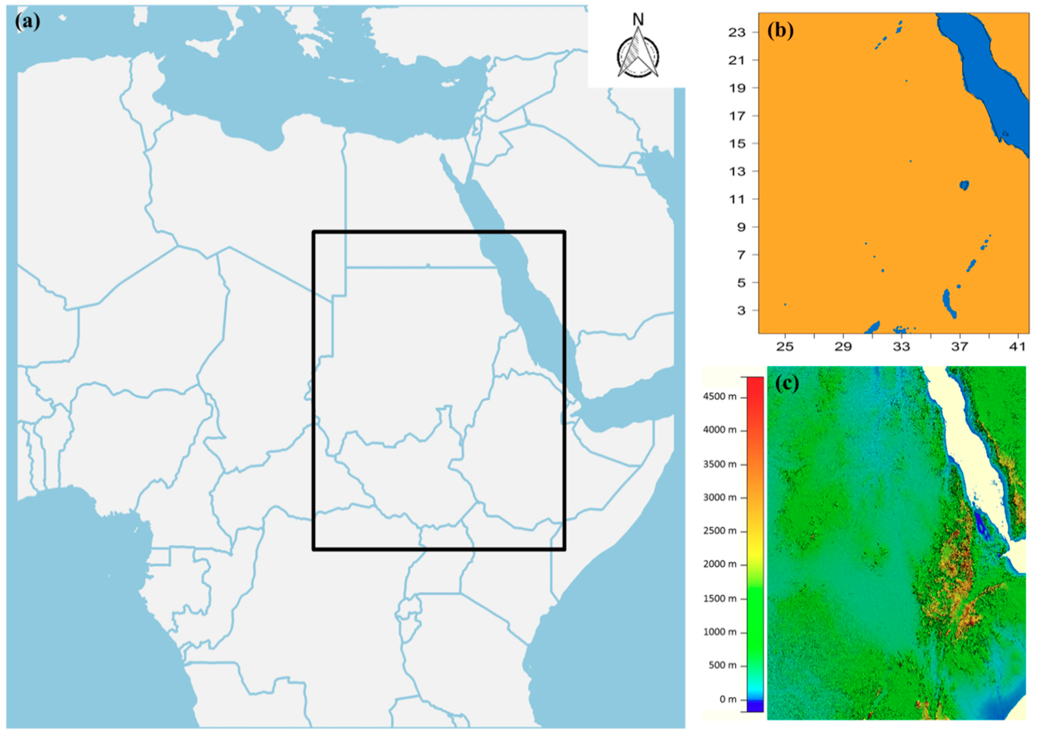
In Egypt, the main source of water at Aswan is the Eastern Nile Basin (ENB), which comprises major rivers with intra-annual flow variability; approximately 85% of the rainfall over the ENB occurs during the rainy season (June to September). The ENB encompasses the Blue Nile, the Tekeze, the Atbara, the Sobat River Basin, and the Baro–Akobo River Basin. Egypt represents about 4% of the total basin area, while Sudan, South Sudan, and Ethiopia represent 13%, 61%, and 22% of the total basin area, respectively, which is illustrated in Figure 1a.

A clear understanding of the current basin climate and hydrological regime as well as the interactions between the two systems is necessary to conduct meaningful climate change projections. This can be achieved by carrying out simulations of the climate/hydrological systems in the basin using numerical modeling techniques.

GCMs are among the most significant tools in use for future projections. GCMs have been used to provide predictions of large-scale climate and general circulation [9,10]. However, they do not resolve local circulation dynamics at the required horizontal resolution of about one degree; higher spatial resolution entails great computational expense. Regional climate models (RCMs) are an alternative, in addition to GCMs, with the advantage that they can achieve higher-resolution simulations over a specific area [11,12,13,14].

Higher resolution can be achieved through dynamic downscaling, where an RCM is forced at its boundaries by meteorological fields. Among many technical considerations, it is first necessary to fine-tune the RCM, so it best reflects the dynamics and the physics of a region of interest. Additionally, the RCM output should first be evaluated against observational data to assess its reliability in capturing spatial and temporal distributions [11,14,15,16], prior to being used in future climate simulations.

Coupling an adjusted RCM over the ENB with a hydrological model will lead to better understanding of the system interactions. This also results in improved coverage of topographical variations, leading to better performance of the hydrological model and ultimately more reliable assessments of the effect of climate change on the ENB stream flow.

Precipitation is considered the most significant aspect of the hydrometeorological cycle in East Africa, in line with evapotranspiration as well as water storage and runoff [17], so a comprehensive investigation is required by considering all these parameters in order to have a better understanding of the hydrometeorological cycle. One way is to conduct such an investigation through atmospheric water balance (AWB) and terrestrial water balance (TWB).

One well-established technique for investigating the above parameters is the water balance calculation (WBC), which can assess the performance of RCMs, examine model uncertainty and determine optimal physics parameterizations to be used. WBC can also be helpful to understand hydrological processes over any area and investigate interactions between atmospheric and hydrological processes. Water balance can be divided into two components: TWB that focuses on surface flows and AWB of those aloft. Jointly considering AWB and TWB relates the change in atmospheric moisture fluxes to precipitation, evapotranspiration, and water storage and runoff [18]; this complex relation can be understood through a water balance study.

Intensive ground observations of hydrometeorological parameters are required for WBC, while the ENB is considered one of the regions that suffer from lack of such data, where the use of RCMs can help obtain the required overview of precipitation, evapotranspiration, radiation energy, humidity, and soil moisture [19,20].

Coupling an optimized RCM with a hydrological model can improve simulations of hydrometeorological parameters [21,22], which can initially be achieved through one-way coupling. With one-way coupling, the hydrological model is forced by meteorological data without any feedback to the atmospheric model, while two-way coupling may be preferred for dynamic climate change studies [23,24]. Studying AWB can be of great benefit for guidance of coupling techniques, depending on precipitation, evapotranspiration, runoff, and moisture fluxes over a study area.

Previous studies have investigated water balance using either atmospheric or terrestrial water storage. Kerandi et al. [25] applied a fully coupled modeling system for the weather research and forecasting (WRF) and WRF-Hydro models over the upper Tana River Basin at Kenya. Two nesting domains were used for the WRF simulation, with spatial resolutions of 25 km and 5 km, respectively, while a 500 m routing resolution was used for the WRF-Hydro model. The AWB and the TWB were considered over both the domains. The precipitation efficiency and the humidity recycling ratio showed close agreement between the two runs, and both of them were close to zero, indicating that most of the precipitation over the region comes from outside the study area. The terrestrial water storage showed seasonal variation, with negative values dominating in January, February, and June, while peak values were seen during April and November. The atmospheric convergence was also the maximum during April and November, which are the peak months of the rainy season. The atmospheric water vapor storage did not show variation on a monthly scale in that regional study, where it had a very small value, near zero, for both the WRF and WRF-Hydro coupled runs.

Roberts et al. [19] investigated the AWB and the TWB for the Churchill River Basin in Canada, using ensembles of regional and global climate models, to develop a clear understanding for the sources of uncertainty in climate models for the North American Regional Climate Change Assessment Program. They calculated the residuals for both the AWB and the TWB; they concluded that the choice of an RCM as well as its parameterizations and customization plays a critical role in determining the residual value, unlike those of a global climate model. According to their work, some sources of uncertainty that need further investigation include the choice of a vertical coordinate system, physics parameterizations, and spectral nudging. The water balance residual was also more consistent for RCMs than for global models.

Seneviratne et al. [26] studied the feasibility of estimating terrestrial water storage on a monthly scale for the Mississippi River Basin, using atmospheric convergence, atmospheric moisture content, and river runoff. ERA-40 meteorological reanalysis was used to provide moisture fluxes and atmospheric water vapor content, while runoff observations were from the United States Geological survey. The monthly terrestrial water storage variation showed excellent agreement with observations in Illinois, including capturing the mean annual cycle and the interannual variation with good accuracy. Over the long term, the variation in terrestrial water storage did not cancel out due to the bias in the reanalysis data. In addition, the variation in monthly soil moisture from the ERA-40 did not match well with the observational data, where underestimation was noted for moisture depletion in summer and recharge in fall, leading to annual cycle damping for soil moisture.

In our study, we focus on estimating the TWB and AWB variables for the ENB, using the output from a previously configured WRF model over the same region; we also assess the performance of the model in simulating some key hydroclimatic variables.

2. Model Setup, Study Area, Datasets, and Methodology

2.1. Model Setup

WRF-ARW version 3.5 [27] was used for a four-year simulation over the period 1998–2001; a six-month spin-up period starting from July 1997 was also added, with these four years considered as a flood period for the basin. The simulation was performed over two nested domains: the parent domain was the MENA-CORDEX region [28], which covers the Middle East and North Africa region with a horizontal spatial resolution of 0.44 degrees (~50 km), and another nested domain centered over the study area with a horizontal spatial resolution of 0.088° (~10 km). All analyses were carried out for the two nested domains.

The model configuration followed the relevant description in Reference [11]; they recommended extent, horizontal spatial resolution, and physics parameterization schemes to be used over the ENB to achieve good performance by the WRF model over this area.

Table 1. Weather research and forecasting (WRF) model configuration parameters for the Eastern Nile Basin (ENB) domain. (CAM: Community Atmospheric Model; MYJ: Mellor-Yamada-Janjic scheme; BMJ: Betts-Miller-Janjic scheme; WSM6: WRF Single Moment 6 classes; NOAH: Noah land surface model).

Extent	Mesh Size	Physics Parameterization
Longitude: 23° E–41.5° E Latitude: 1.5° N–24.5° N	Parent grid ratio: 1:5 Resolution: 0.088° (~10 km) No. of cells: 196 × 251 × 30	Shortwave radiation: CAM Longwave radiation: CAM Planetary boundary layer: MYJ Cumulus convection: BMJ Microphysics: WSM6 Land surface model: NOAH

summarizes the model configuration parameters.

Regarding the driving data, ERA-Interim reanalysis data [29] were used to force the MENA-CORDEX domain with relative and specific humidity, temperature, geopotential, and horizontal wind components at each pressure level, while at each soil level temperature, moisture, and surface parameters (i.e., surface horizontal wind components, surface geopotential, Mean sea level pressure, sea–ice fraction, skin temperature, snow depth, SST, T2M, and T2M dew) were used. The MODIS 20-category land cover product was used in order to represent the land cover [30]. The Noah land surface model (NOAH) was used to represent land surface processes [31].

2.2. Study Area

The ENB encompasses Egypt, Sudan, South Sudan, and Ethiopia. It covers an area of approximately 1,809,606 square kilometers; the elevation within the basin varies from 100 to close to 4500 m. The basin experiences two different climate regimes: the northern part being arid and semiarid and the rest of the domain being tropical or subtropical. The land cover within the basin has not changed significantly over the past several decades. Figure 1 shows the domain extent used to cover the ENB, the area topography, and the land mask.

2.3. Observational Datasets

In order to assess the model performance in simulating atmospheric variables such as precipitation and surface air temperature, the following gridded datasets were used. The Global Precipitation Climatology Center (GPCC) version 7 [32] dataset provides monthly total precipitation available at a spatial resolution of 0.5° × 0.5°. The region of interest was characterized by strong observational uncertainty with regards to the gridded precipitation datasets. Nevertheless, the GPCC dataset was found to be in good agreement with other datasets for our simulation period [33]. The University of Delaware (UDEL) version 5.01 dataset was used for investigating surface air temperature [34]. Since the horizontal resolution of the study area differs from the spatial resolution of the gridded datasets, the observational datasets were regridded to the domain horizontal resolution in order to facilitate the comparison.

2.4. Methodology

2.4.1. Atmospheric Water Balance

In the AWB, the water vapor flowing into and out of the atmosphere is represented over a certain region. Water is added to the atmosphere through either evaporation or transpiration, and it is removed from the atmosphere by means of precipitation.

A simple mass balance equation can be used to describe the mass conservation of water vapor in the atmosphere, shown as Equation (1) [19,35,36,37]:

$$\frac{\mathrm{dW}}{\mathrm{dt}}=-\nabla ·\mathrm{Q}+\mathrm{ET}-\mathrm{P},$$

(1)

where dW/dt represents the total change in perceptible water content in the atmosphere or the change in the amount of water vapor stored in the atmosphere; ∇·Q represents the mean convergence of the lateral atmospheric water vapor flux (calculated by: outflux–influx); ET represents evapotranspiration; and P represents precipitation. For more calculations using Equation (1), please refer to [19,35,36,37].

Some terms in Equation (1) are derived directly from the WRF model, and the others can be derived as a function of the model output. For example, precipitation is a direct model output. Evapotranspiration can be calculated as a ratio between the latent heat flux at the surface and the latent heat of the vaporization of water, which is a function of temperature. The mean convergence of the lateral atmospheric water vapor flux can be calculated as the difference between the lateral water vapor outflow across the lateral boundary domain and the lateral water vapor inflow across the lateral boundary domain.

Horizontal, lateral fluxes were calculated by multiplying the water vapor mixing ratio (which refers to absolute humidity) at each grid point with two velocity components (East–West and North–South directions) to obtain two flux values for each grid point at four boundaries, followed by the calculation of the humidity flux that either leaves the domain or enters it at each boundary grid point, depending on the two fluxes. Then, vertical integration takes place for all the layers, resulting in a value for the influx and outfluxes at each time step. More details for calculations of atmospheric convergence can be found in Reference [26]. Over the long term, dW/dt approaches zero. The accuracy of Equation (1) depends on the size of a domain under consideration, as noted by Rasmusson [35]; the domain area should be around 2 × 10⁶ km² in order to have consistent results.

In order to analyze the atmospheric fluxes and the regional water cycle over the ENB, two additional bulk characteristics were used following References [25,38,39,40]: precipitation efficiency (χ) and moisture recycling ratio (β).

The precipitation efficiency refers to the amount of precipitation falling onto the domain as a result of moisture entering the atmosphere from either evapotranspiration or inflow of moisture from outside. The moisture recycling ratio refers to the fraction of precipitation originating solely from evapotranspiration within the domain. Equations (2) and (3) describe the precipitation efficiency and the recycling ratio, respectively, which can be shown as following:

$$\mathsf{\chi }=\frac{\mathrm{P}}{\mathrm{ET}+\mathrm{IN}},$$

(2)

$$\mathsf{\beta }=\frac{\mathrm{ET}}{\mathrm{ET}+\mathrm{IN}},$$

(3)

where IN is the moisture flux inflow to the domain from the lateral boundary. The mixing ratio and the precipitation efficiency must be averaged over a long time period (e.g., a month), so that the moisture storage in the atmosphere can be assumed to be neglected.

2.4.2. Terrestrial Water Balance

Equation (4) describes the TWB and can be used to check the balance of the water cycle on the ground surface, which was written as:

$$\frac{\mathrm{dS}}{\mathrm{dt}}=-\mathrm{R}-\mathrm{ET}+\mathrm{P},$$

(4)

where dS/dt represents the total change in the terrestrial water storage; R represents the total runoff, which is the difference between the in- and out-runoff; ET represents evapotranspiration and P represents precipitation.

Precipitation and total runoff can be used directly from the results of the WRF model; for evapotranspiration, the method described above will be used again, with the latent heat fluxes at the surface divided by the latent heat of the vaporization of water.

3. Results

3.1. Precipitation

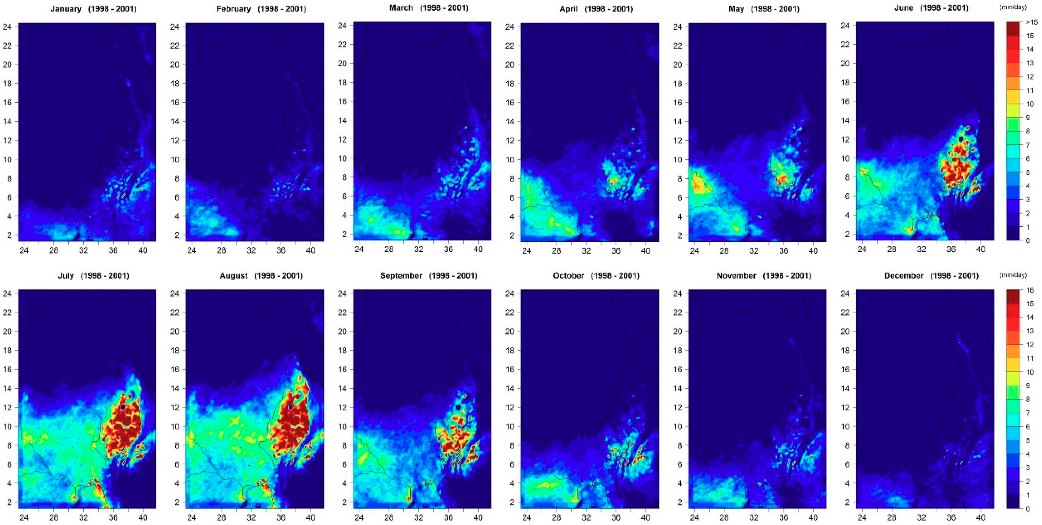
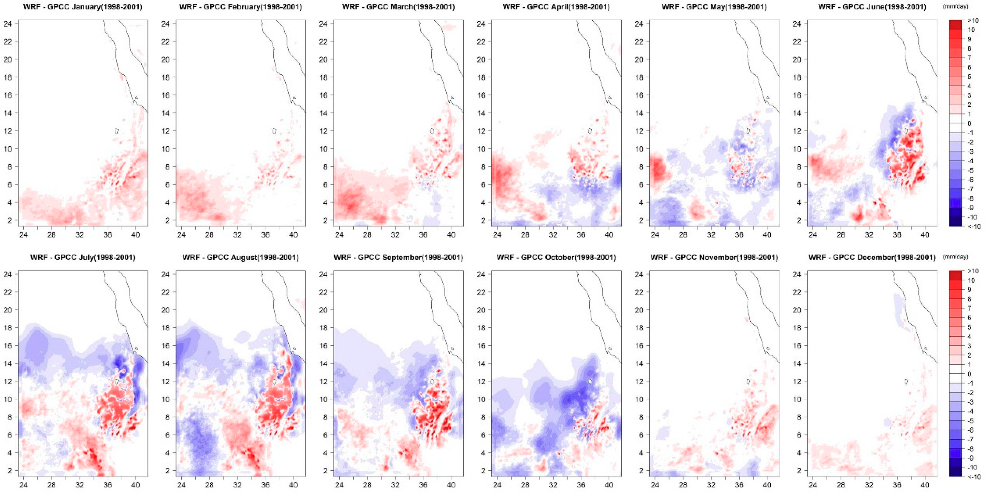
Simulated precipitation from the WRF model was investigated first. Figure 2 shows the mean daily precipitation by month, averaged over the study period, with the rainiest months for the ENB being June, July, August, and September, while December, January, February, and March can be considered the dry season. During the rainy season, most precipitation falls on the Ethiopian Highlands (35–41° E, 5–14° N), where the model simulates precipitation with values that reach 25 mm/day for some grid points. The northern part of the ENB seems to be dry, with precipitation values less than 1 mm/day over the entire year. To assess the model performance in simulating precipitation, bias values were calculated using the GPCC dataset (see Figure 3). The model overestimates the precipitation, especially over the highlands, with values reaching 10 mm/day during the rainy season. Averaging total precipitation over the Ethiopian Highlands improves the comparison, with a mean total precipitation of 6.7 mm/day during the entire rainy season using the WRF simulation versus that of 5.8 mm/day using the GPCC dataset. For the entire domain, the average precipitation drops to 2.7 mm/day with the WRF simulation during the rainy period and 2.8 mm/day using the GPCC dataset; again, these two average precipitation values are consistent.

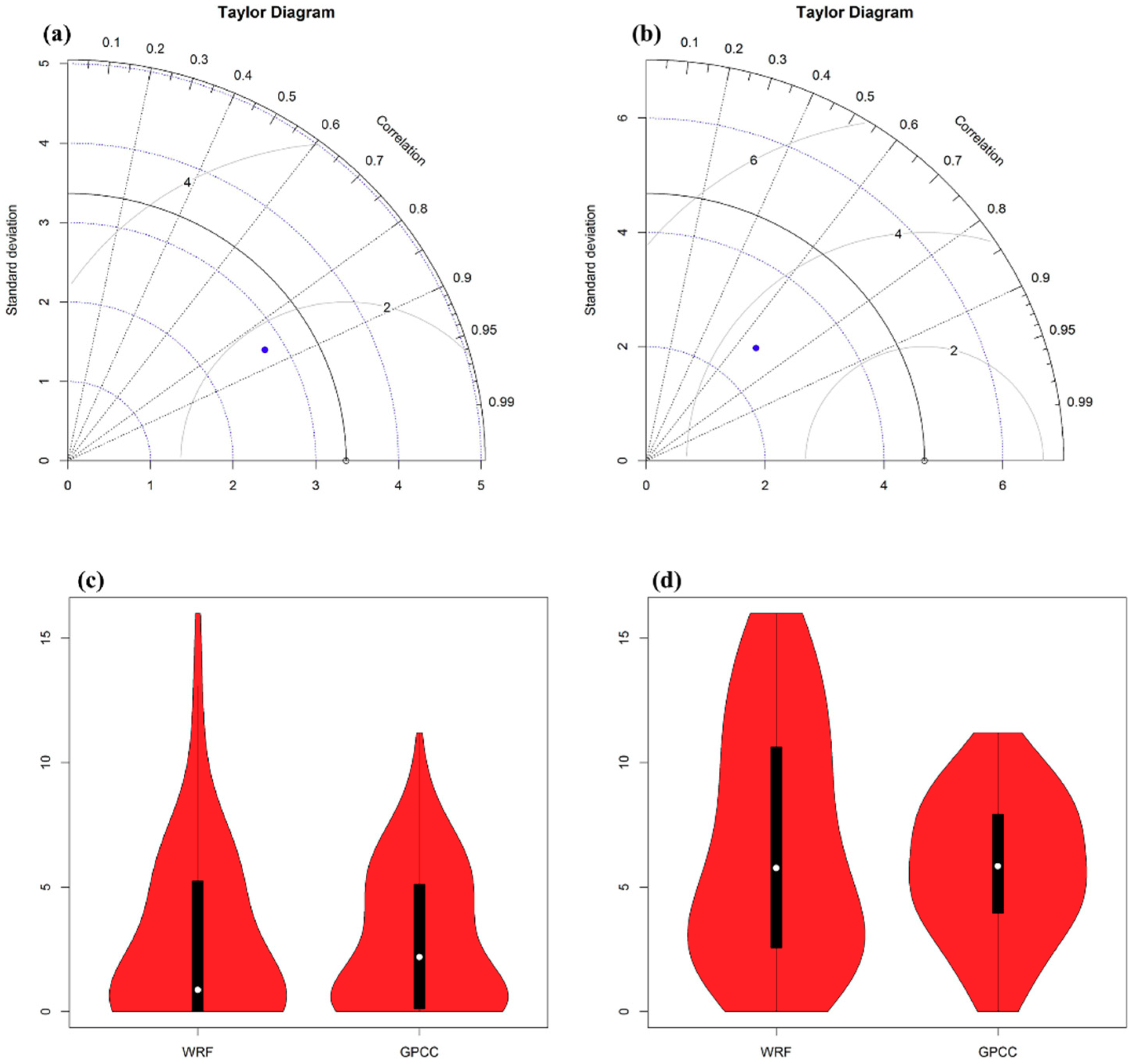
Further analysis is shown in Figure 4; a Taylor diagram [41] is presented for the entire domain and the Ethiopian Highlands. With respect to the whole domain, the correlation coefficient is 0.87, the standard deviation is 2.6 mm/day, and the centered root mean square error is 1.7 mm/day for the mean daily precipitation during the rainy season averaged over the study period. Such the values indicate good performance of the WRF simulation. By focusing these metrics on the Ethiopian Highlands, the correlation coefficient becomes 0.68, the standard deviation is 2.4 mm/day, and the centered root mean square error is 3.4 mm/day.

The bottom panels of Figure 4 show violin plots, indicating good agreement between the precipitation distributions of the GPCC dataset and the WRF simulations. Note that a violin plot is a combination of a boxplot and a kernel density plot that provides the minimum and maximum values as well as lower, middle, and upper quartiles; it also gives the probability density function smoothed by a kernel density estimator [42].

For the entire domain, the density function has nearly the same distribution, with the exception of the highest precipitation values of 16 mm/day obtained with the simulation and approximately 12 mm/day from the GPCC dataset. However, the median value is much lower than the average value with the simulation, indicating a skewed distribution using the simulation. For the Ethiopian Highlands, the probability density function shows some differences between the simulated precipitation and that from the GPCC dataset.

3.2. Temperature

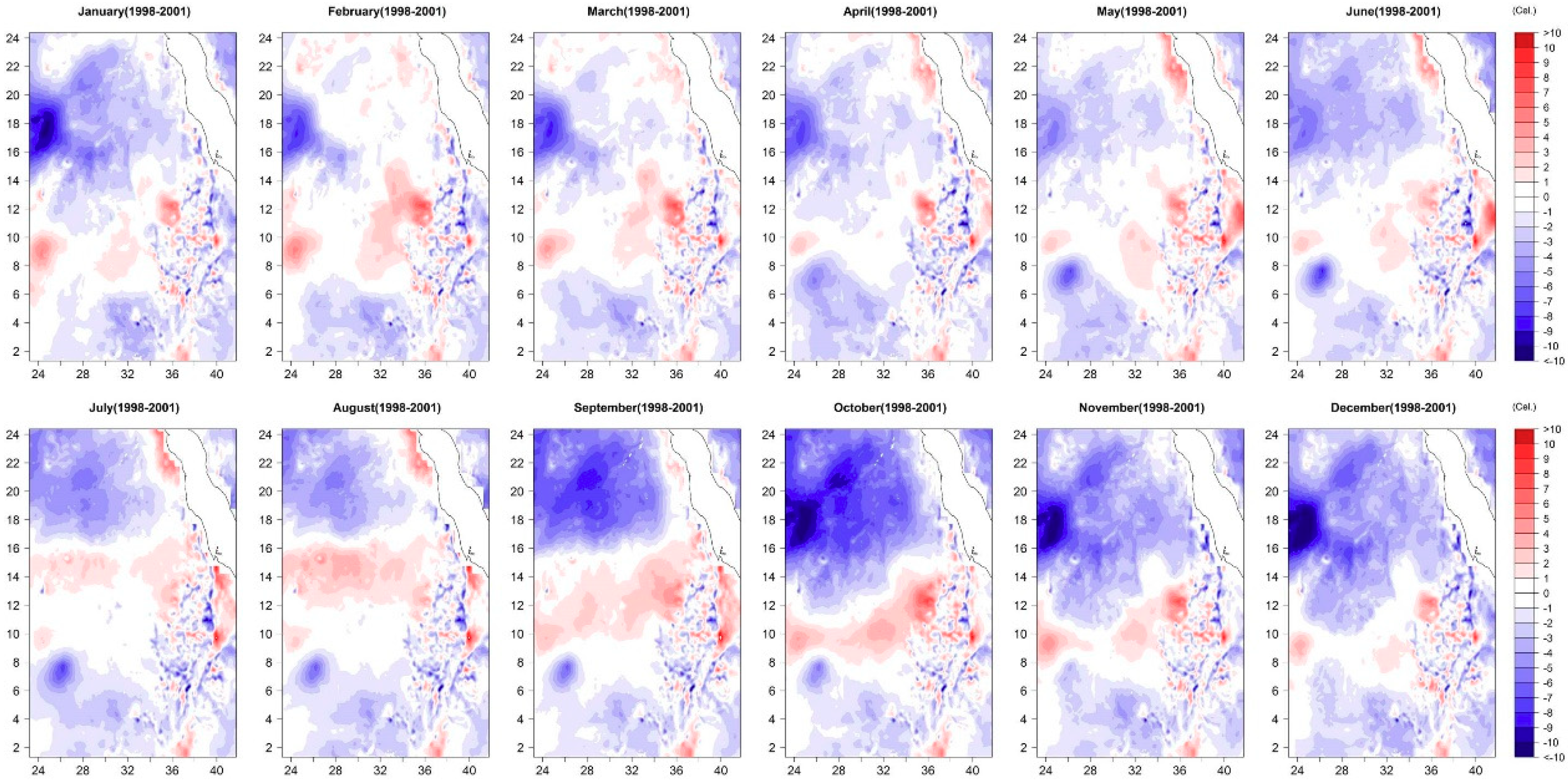
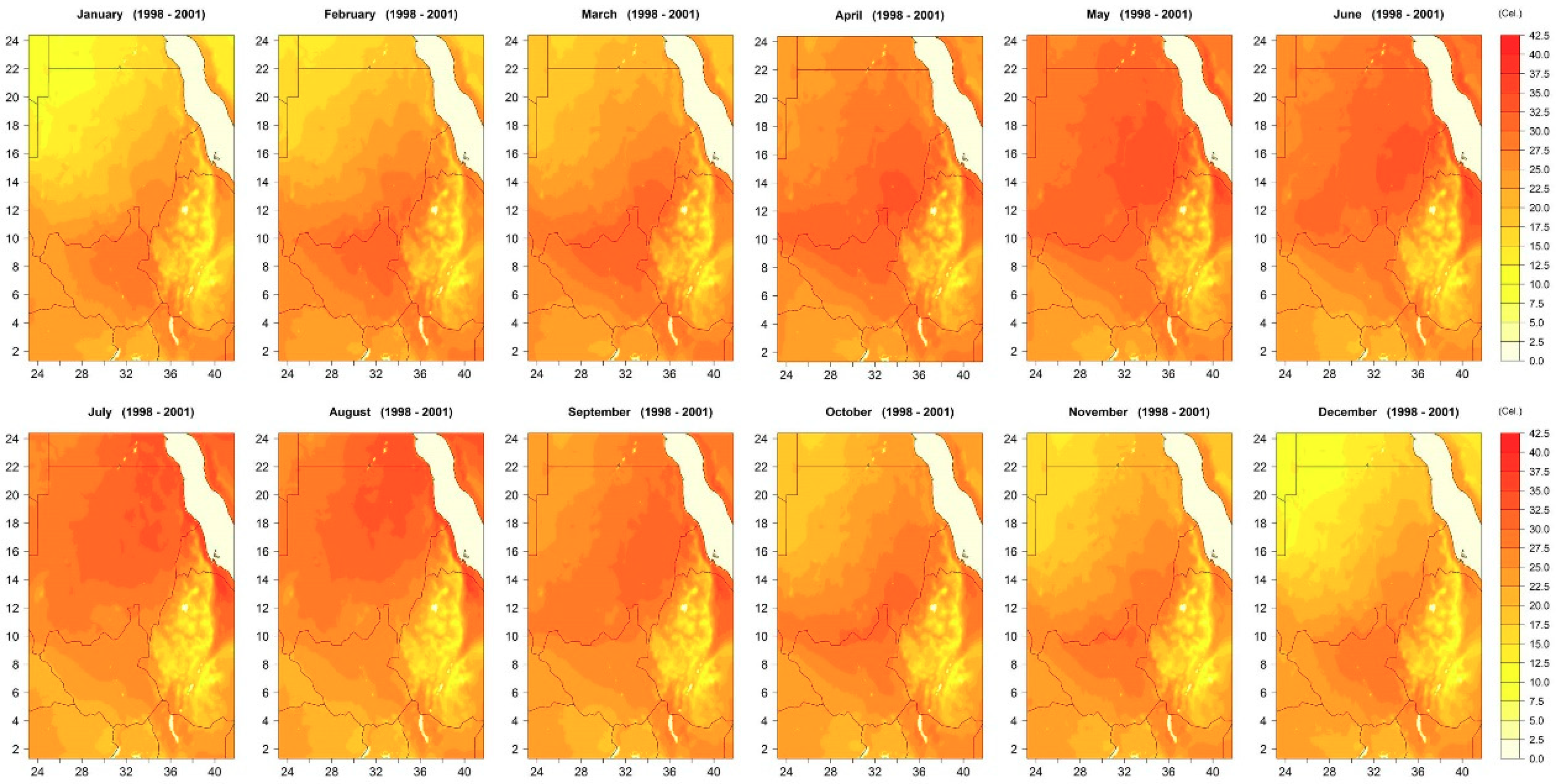
The WRF model appears to perform well in simulating surface air temperature over the ENB. Figure 5 presents the simulated average surface air temperature based on the WRF model results for all the months, and Figure 6 shows the bias between the simulated data and the surface air temperature from the UDEL dataset for all the months. The simulated mean monthly temperature ranges between 10 and 38 °C, with small exceptions for some grid points. The northern part of the domain usually has higher temperature than the southern part, except during the dry season, when the northern part experiences lower temperatures. In terms of bias, the northern part underestimates the simulated temperature throughout the year, with a bias up to a 10 °C difference between the simulated temperature and the temperature from the gridded dataset at some grid points, especially during the period from October to January.

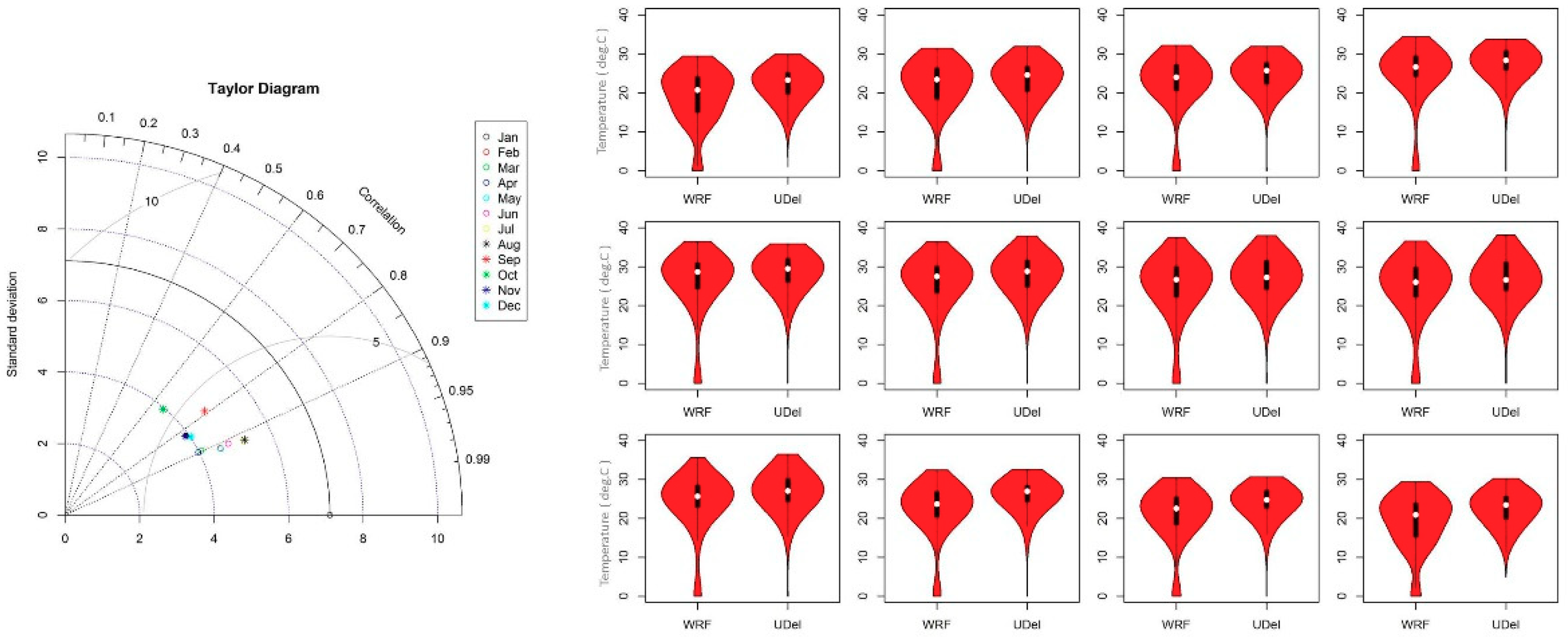
Figure 7 presents a Taylor diagram for the average monthly temperature during the study period. A correlation coefficient greater than 0.9 was found in most of the months, except for September, November, and December, in which the correlation coefficient ranges from 0.8 to 0.9; the weakest correlation was found in October. The standard deviation is less than 6 °C for the whole year, and the center root mean square error is less than 5 °C in all the months, except for October. The violin plots show good agreement between the simulated temperatures and those from the UDEL dataset in terms of density distribution and quartiles, with differences of the mean temperatures between the simulations and the UDEL dataset not exceeding 3 °C.

3.3. Evapotranspiration

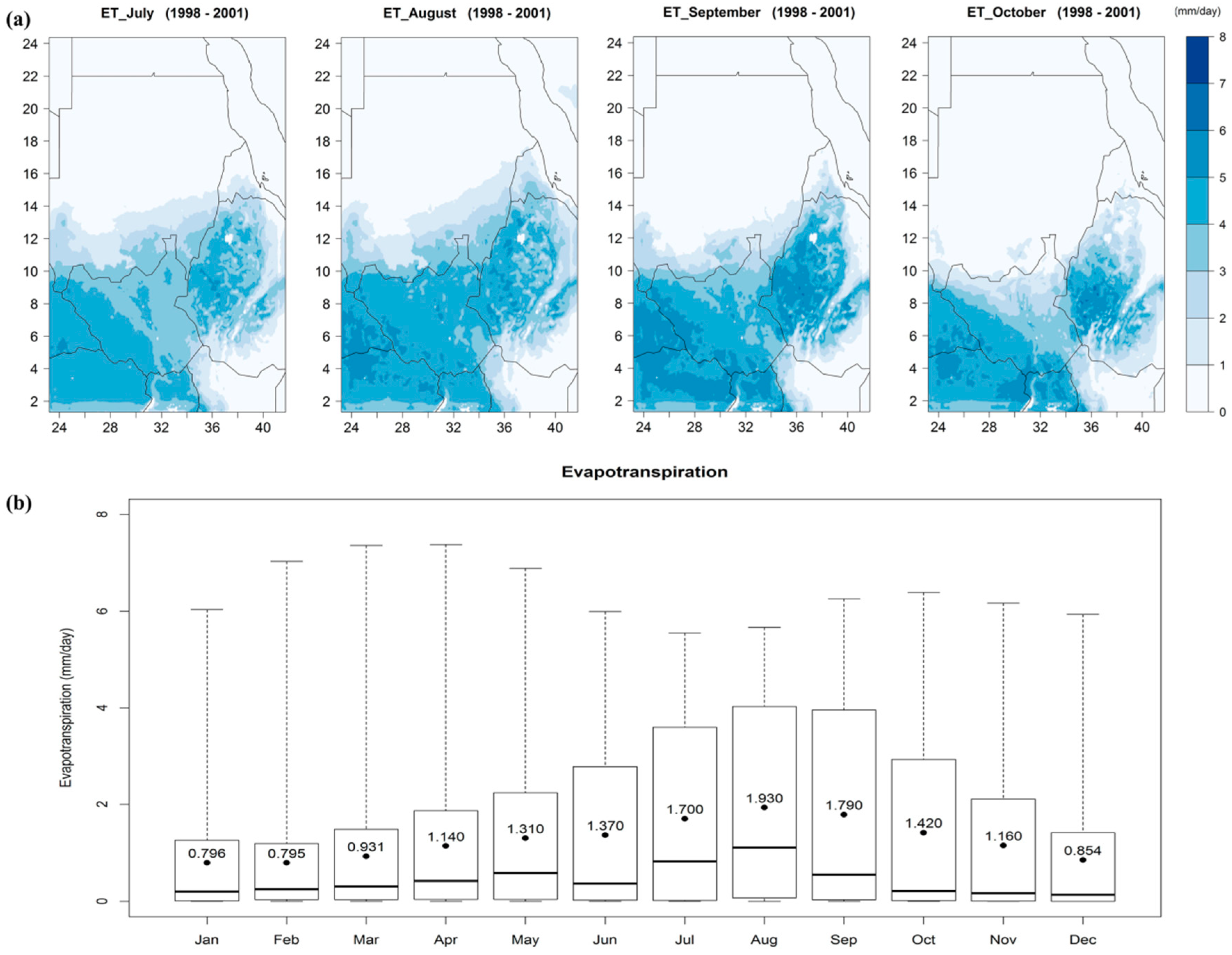
Evapotranspiration was calculated by dividing the latent heat flux at the surface by the latent heat of the vaporization for water, which is a function of temperature. The ENB can be divided into two regions for evapotranspiration: the northern region encompassing Egypt and Sudan and the remaining area of the basin. The northern region is classified as arid, with evapotranspiration less than 0.5 mm/day throughout the year. In the remaining region, evapotranspiration ranges between 0 and 7 mm/day for some months.

Figure 8 shows the mean land evapotranspiration during July, August, September, and November, in which the highest evapotranspiration values were found. In contrast, the minimum values were found during December, January, and February. Figure 8 also presents boxplots for land evapotranspiration over the entire domain. The highest mean land evapotranspiration value of 1.93 mm/day was identified in August, while a mean value of about 0.79 mm/day was found in January and February. These results agree well with the MODIS global evapotranspiration data (MOD16) [43]; the seasonal variations of the evapotranspiration and the mean monthly values are to some extent overestimated in the simulated evapotranspiration for some grid points, but the bias is very small on the mean monthly scale and does not exceed 1 mm/day.

3.4. Runoff

Surface runoff from the WRF model was also analyzed in order to determine the TWB according to equation 4. The simulated runoff values are given by the land surface model as the total depth of water at each grid point without any routing modules that can calculate surface flow. Follow-up studies coupling the WRF model with a hydrological model will have the ability to calculate the surface and channels flows.

Figure 9 presents maps of the average runoff for the months with the highest mean runoff and boxplots depicting the runoff distributions and the means for all the months. The runoff reaches its peak value of 0.656 mm/day during August for the entire domain, but for the Ethiopian highlands the runoff value is up to 10 mm/day for some grid points.

The arid part of the domain seems to have no runoff throughout the year. During December, January and February, the mean runoff values do not exceed 0.1 mm/day for the entire domain. The temporal and spatial variation of runoff is consistent with that of the precipitation distribution, especially during the rainy season.

3.5. Terrestrial Water Balance

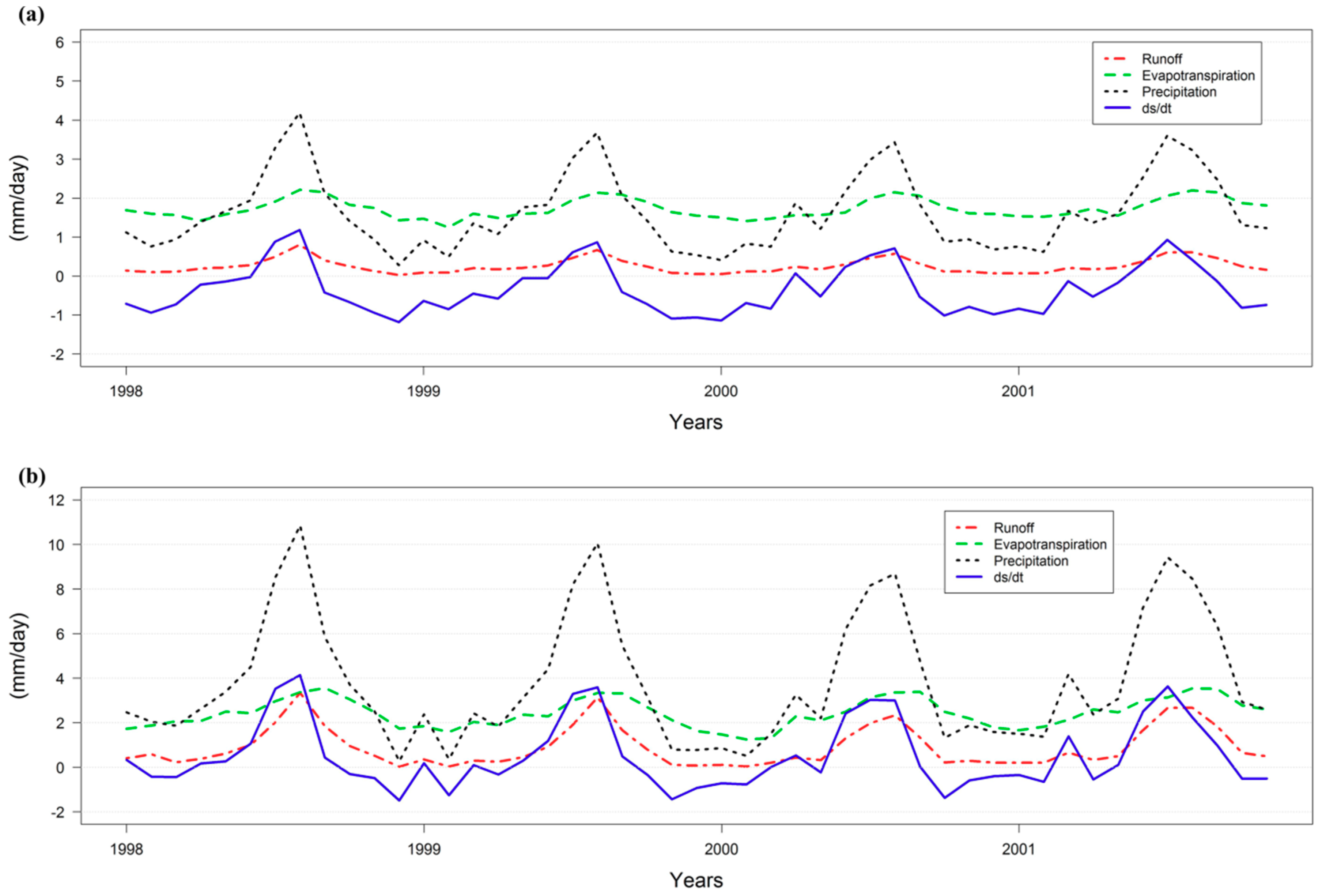
Using Equation (4), all the terms were integrated on a monthly time scale during the study period and are expressed as an average (unit: mm/day) for each month. Figure 10 presents time series for the runoff, the evapotranspiration, the precipitation, and the terrestrial water storage for both the entire ENB domain and the Ethiopian Highlands. For the entire domain, dS/dt showed seasonal variation, ranging from −1.18 to 1.18 mm/day, with a mean of −0.35 mm/day for the entire study period. Negative values were found in most of the months, with the exception of June, July, and August, when most of the precipitation falls. August is the month with the highest positive average dS/dt value during the whole study period, while December is the month with the lowest average dS/dt value.

Table 2. Average change in terrestrial water storage for each month.

Month	dS/dt (mm/day)
	The Entire Domain	The Ethiopian Highlands
January	−0.83	−0.14
February	−0.86	−0.78
March	−0.54	0.27
April	−0.32	−0.04
May	−0.22	0.11
June	0.12	1.79
July	0.74	3.37
August	0.80	3.24
September	−0.37	0.49
October	−0.80	−0.63
November	−0.89	−0.75
December	−1.07	−0.94
Average	−0.35	0.50

presents an average value of dS/dt for each month during the study period for the entire ENB domain.

In the Ethiopian Highlands, the terrestrial reservoir appears to have a higher water storage rate than the other regions within the domain, because most of the precipitation over the basin occurs over the Ethiopian Highlands; moreover, the runoff and the evapotranspiration are higher in that region. In the Ethiopian Highlands, dS/dt varied seasonally, ranging from −1.49 to 4.14 mm/day with a mean of 0.5 mm/day for the entire period. The highest dS/dt value was observed during July and August, with values of 3.37 mm/day and 3.24 mm/day, respectively; the lowest dS/dt value of −0.94 mm/day was again found in December. Table 2 lists the average values of dS/dt for the Ethiopian Highlands; positive storage rates for the terrestrial water were found in most of the months.

A comparison of the terrestrial water storage for the entire domain and for the Ethiopian Highlands indicates the same seasonal pattern, with higher positive values and fewer negative values for the Ethiopian Highlands.

3.6. Atmospheric Water Balance

Moisture fluxes were calculated at each boundary of the domain in order to integrate the lateral atmospheric water vapor flux. Based on the moisture fluxes from each boundary, the eastern boundary contributes the largest moisture flux to the study domain, especially from June to September; the average moisture influx during these months is 185 mm/day. The eastern boundary also contributes approximately 40% of the moisture outflux over the whole study period, especially from January to April.

The northern boundary seems to contribute little in terms of moisture fluxes to the domain; the average in- and outfluxes are less than 8 mm/day. Thus, this boundary contributes only 3.1% and 2.8% of the in- and outfluxes, respectively. This result is expected, because this boundary is within an arid and semiarid region. The southern boundary is a source of moisture year-round, with an average value of 18 mm/day for the moisture flux inflow. The western boundary can be considered a moisture sink for the domain, especially from June to September, with an average value of 177 mm/day for the moisture outflux.

Table 3. Percentages of the moisture in- and outfluxes from each boundary.

Boundary	Moisture Flux (%)
	In	Out
Eastern	57.1	40.2
Western	25.8	57.0
Northern	3.1	2.8
Southern	14.0	0.0

shows the percentages of the moisture in- and outfluxes from each boundary.

The atmospheric circulation over Africa is characterized by the annual progression of the intertropical convergence zone, the extratropical influences to the south, and the seasonally varying monsoon winds [44]. Especially in East Africa, the region is dominated by the monsoon circulation and the seasonal migration of the intertropical convergence zone.

Most of the moisture influxes are from the eastern boundary, mainly during the rainy season, where the impact of transport from the Indian Ocean is relatively strong. The moisture influxes during the rainy season, which fuel more than 50% of the precipitation over the region, seem to be closely linked to the strength of the Wyrtki jet in the upper Indian Ocean, forced by the surface wind in a westerly direction, which reinforce the ocean temperature gradient in the east–west direction and form part of the equatorial zonal circulation [45]. Accordingly, most of the moisture flux exchanges are from the western and eastern boundaries of the domain, as shown in Table 3.

Atmospheric convergence of the lateral moisture flux is defined as the difference between the outflux and the influx from the boundary, which can be written as: outflux from the boundary – influx from the boundary). The ENB domain is a sink for moisture, with negative values for most of the months. The greatest atmospheric convergence was noted in July and August, with an average of −1.38 mm/day; these months represent the peak of the rainy season. The lowest values for the convergence were found in January and February. The average total convergence over the entire study period is approximately −0.3 mm/day.

No monthly or annual cycle is evident in terms of total change in atmospheric water content; the change in perceptible water content in the atmosphere was low throughout the year, with an average during the rainy season of 0.1 mm/day and some negative values in some rainy months. In the dry season, the average is 0.03 mm/day. The values for the total change of the atmospheric water content are expected to be very small and approach zero.

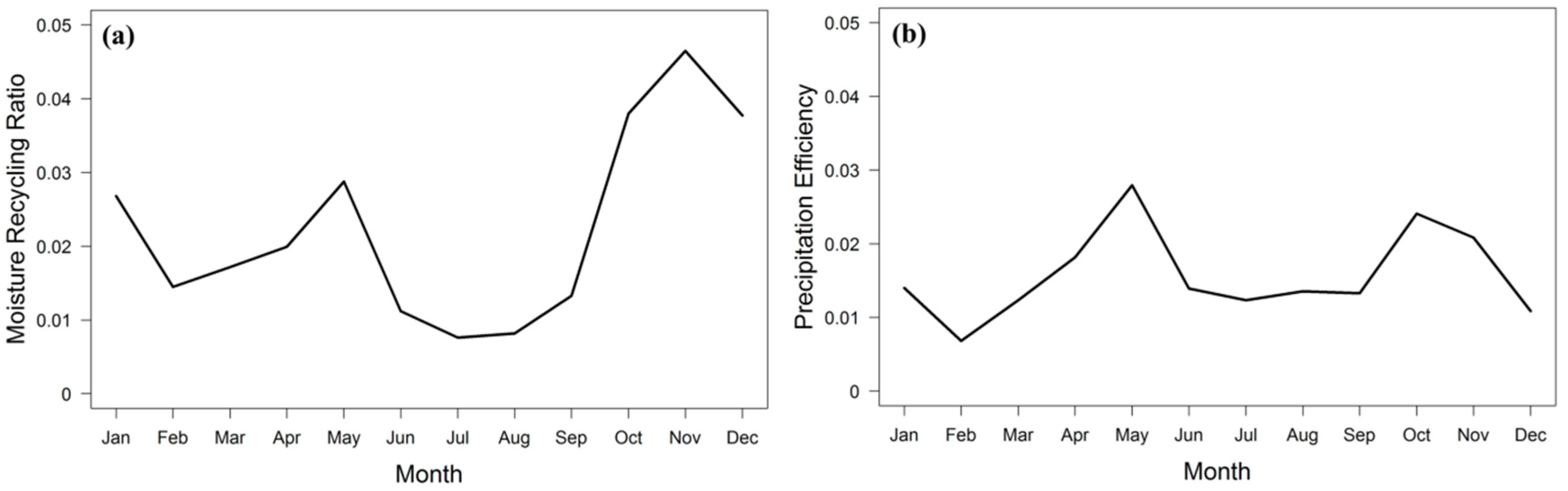
Figure 11 shows the annual cycle for both the precipitation efficiency and the moisture recycling ratio. The moisture recycling ratio is very small throughout the year, with values less than 0.05, meaning that most of the precipitation in the area originates from outside the domain and does not depend on the local evapotranspiration. Such small values of the recycling ratio mean that the precipitation over the area does not greatly rely on land surface processes within the region or on the land–precipitation link. Thus, a significant difference in the precipitation values is not expected, if the atmospheric model is coupled with a hydrological model.

In terms of the annual cycle of the recycling ratio, mean values are generally high for evapotranspiration, with the lowest values for the recycling ratio in July and August when the moisture inflow into the domain is high during the rainy season and with higher values in November, December and January, when there is less moisture inflow into the domain. Further, the variation in the evapotranspiration is not controlling the annual cycle; the evapotranspiration is very low compared to the moisture flux inflow, which may reach a hundred times the evapotranspiration value.

The precipitation efficiency was quite low, with an annual cycle similar to that of the moisture recycling ratio due to high values of the moisture influx compared to those of the evapotranspiration and the precipitation; in contrast, during the dry season, the precipitation is very low relative to the precipitation efficiency and the values were lower than the recycling ratio. Small values of the precipitation efficiency mean that only a small portion of the moisture flux inflow contributes to most of the precipitation over the ENB.

4. Conclusions

A water balance study was carried out for the ENB region using the output from the WRF model applied over a period of four years. The model results were compared with the gridded precipitation data in order to assess the model performance before applying the water balance.

For the simulated precipitation, the modeled convective and nonconvective precipitation values were compared against the GPCC dataset; the model shows a positive bias up to 10 mm/day during the rainy season. For the average precipitation over the Ethiopian Highlands, the average of 6.7 mm/day throughout the rainy season for the WRF simulation is close to that of 5.8 mm/day observed from the GPCC dataset. For the entire domain, the average precipitation is 2.7 mm/day for the WRF simulation during the rainy period, which is very close to 2.8 mm/day observed from the GPCC dataset; the temporal correlation coefficient is 0.87 for the entire study area.

Most of the months show a high temporal correlation coefficient for the surface air temperature, with values greater than 0.9 and a center root mean square error less than 5 °C. Evapotranspiration was calculated from the output of the model by dividing the latent heat fluxes at the surface by the latent heat of the vaporization for water, which is a function of temperature. The simulated evapotranspiration in the northern part of the domain is less than 0.5 mm/day throughout the year, while for the remaining regions the evapotranspiration ranged from 0 to 7 mm/day.

To investigate both the TWB and the AWB, the computations for each component were performed: evapotranspiration, precipitation, and runoff were used to calculate the change in the terrestrial water storage, and evapotranspiration, precipitation, and atmospheric moisture convergence were used to calculate the total change in the perceptible water content in the atmosphere.

The results showed that the change in terrestrial water storage does show a significant seasonal variation (−1.18 to 1.18 mm/day), with a mean value of −0.35 mm/day for the entire study period. Negative values were found in most of the months, except June, July, and August, when most of the precipitation occurs. As expected, the change in atmospheric moisture content shows little variation, with very small values approaching zero during the entire study period.

The ENB is a sink for moisture, with negative values of the atmospheric convergence for most of the months. The contribution of the local evapotranspiration to the precipitation was very small, and most of the precipitation originates from outside the domain, as reflected in the small value for the moisture recycling ratio.

Finally, the overall performance of the WRF model over the ENB seems to be quite satisfactory in reproducing precipitation, temperature, and evapotranspiration according to the statistical metrics used and the AWB results. The encouraging results pave a way for developing coupled hydrological and atmospheric modeling and performing scenario calculations of the hydroclimate in the region, including river flows and surface runoff, which are of key relevance for water and food security in the area.

References

1. Swain, A. Challenges for water sharing in the Nile Basin: Changing geo-politics and changing climate. Hydrol. Sci. J. 2011, 56, 687–702. [Google Scholar] [CrossRef]
2. Conway, D.; Hulme, M. The impacts of climate variability and future climate change in the Nile basin on water resources in Egypt. Water Resour. Dev. 1996, 12, 277–296. [Google Scholar] [CrossRef]
3. Yates, D.N.; Strzepek, K.M. Modeling the Nile Basin under climatic change. J. Hydrol. Eng. 1998, 3, 98–108. [Google Scholar] [CrossRef]
4. Conway, D. From headwater tributaries to international river: Observing and adapting to climate variability and change in the Nile Basin. Glob. Environ. Chang. 2005, 15, 99–114. [Google Scholar] [CrossRef]
5. Beyene, T.; Lettenmaier, D.P.; Kabat, P. Hydrologic impacts of climate change on the Nile River basin: Implications of the 2007 IPCC scenarios. Clim. Chang. 2010, 100, 433–461. [Google Scholar] [CrossRef]
6. Elshamy, M.; Seierstad, I.A.; Sorteberg, A. Impacts of climate change on Blue Nile flows using bias-corrected GCM scenarios. Hydrol. Earth Syst. Sci. 2009, 13, 551–565. [Google Scholar] [CrossRef]
7. Soliman, E.S.A.; Sayed, M.A.A.; Nour El-Din, M.M.; Samy, G. Integration of NFS with Regional Climate Model to Simulate the Nile Basin Hydro-climatology. Nile Basin Water Eng. Sci. Mag. 2008, 1, 75–85. [Google Scholar]
8. Githui, F.; Gitau, W.; Mutua, F.; Bauwens, W. Climate change impact on SWAT simulated streamflow in western Kenya. Int. J. Climatol. 2009, 29, 1823–1834. [Google Scholar] [CrossRef]
9. Gillett, N.P.; Thompson, D.W. Simulation of recent Southern Hemisphere climate change. Science 2003, 302, 273–275. [Google Scholar] [CrossRef]
10. Solomon, S.; Qin, D.; Manning, M.; Averyt, K.; Marquis, M. (Eds.) Climate Change 2007-The Physical Science Basis: Working Group I Contribution to the Fourth Assessment Report of the IPCC; Cambridge University Press: Cambridge, UK, 2007; Volume 4. [Google Scholar]
11. Abdelwares, M.; Haggag, M.; Wagdy, A.; Lelieveld, J. Customized framework of the WRF model for regional climate simulation over the Eastern NILE basin. Theor. Appl. Climatol. 2018, 134, 1135–1151. [Google Scholar] [CrossRef]
12. Fu, C.; Wang, S.; Xiong, Z.; Gutowski, W.J.; Lee, D.K.; McGregor, J.L.; Suh, M.S. Regional climate model intercomparison project for Asia. Bull. Am. Meteorol. Soc. 2005, 86, 257–266. [Google Scholar] [CrossRef]
13. Giorgi, F. Climate change hot-spots. Geophys. Res. Lett. 2006, 33. [Google Scholar] [CrossRef]
14. Laprise, R. Regional climate modelling. J. Comput. Phys. 2008, 227, 3641–3666. [Google Scholar] [CrossRef]
15. Kostopoulou, E.; Tolika, K.; Tegoulias, I.; Giannakopoulos, C.; Somot, S.; Anagnostopoulou, C.; Maheras, P. Evaluation of a regional climate model using in situ temperature observations over the Balkan Peninsula. Tellus A Dyn. Meteorol. Oceanogr. 2008, 61, 357–370. [Google Scholar] [CrossRef]
16. Leung, L.R.; Mearns, L.O.; Giorgi, F.; Wilby, R.L. Regional climate research: Needs and opportunities. Bull. Am. Meteorol. Soc. 2003, 84, 89–95. [Google Scholar]
17. Endris, H.S.; Omondi, P.; Jain, S.; Lennard, C.; Hewitson, B.; Chang’a, L.; Awange, J.L.; Dosio, A.; Ketiem, P.; Nikulin, G.; et al. Assessment of the performance of CORDEX regional climate models in simulating East African rainfall. J. Clim. 2013, 21, 8453–8475. [Google Scholar] [CrossRef]
18. Eltahir, E.A.B.; Bras, R.L. Precipitation recycling. Rev. Geophys. 1996, 34, 367–378. [Google Scholar] [CrossRef]
19. Roberts, J.; Snelgrove, K. Atmospheric and terrestrial water balances of Labrador’s Churchill River basin, as simulated by the North American Regional Climate Change Assessment Program. Atmos. Ocean 2015, 53, 304–318. [Google Scholar] [CrossRef]
20. Music, B.; Caya, D. Evaluation of the hydrological cycle over the Mississippi River basin as simulated by the Canadian Regional Climate Model (CRCM). J. Hydrometeorol. 2007, 8, 969–988. [Google Scholar] [CrossRef]
21. Senatore, A.G.; Mendicino, D.J.; Gochis, W.; Yu, D.N.; Kunstmann, H.Y. Fully coupled atmosphere hydrology simulations for the central Mediterranean: Impact of enhanced hydrological parameterization for short and long time scales. J. Adv. Model. Earth Syst. 2015, 7, 1693–1715. [Google Scholar] [CrossRef]
22. Ryu, Y.; Lim, Y.J.; Ji, H.S.; Park, H.H.; Chang, E.C.; Kim, B.J. Applying a coupled hydrometeorological simulation system to flash flood forecasting over the Korean Peninsula. Asia-Pacific J. Atmos. Sc. 2017, 53, 421–430. [Google Scholar] [CrossRef]
23. Wagner, S.B.; Fersch, F.; Yuan, Z.; Kunstmann, H.Y. Fully coupled atmospheric hydrological modeling at regional and long-term scales: Development, application, and analysis of WRF-HMS. Water Resour. Res. 2016, 52, 3187–3211. [Google Scholar] [CrossRef]
24. Naabil, E.; Lamptey, B.L.; Arnault, J.; Olufayo, A.; Kunstmann, H. Water resources management using the WRF-Hydro modelling system: Case-study of the Tono dam in West Africa. J. Hydrol. Reg. Stud. 2017, 12, 196–209. [Google Scholar] [CrossRef]
25. Kerandi, N.; Arnault, J.; Laux, P.; Wagner, S.; Kitheka, J.; Kunstmann, H. Joint atmospheric-terrestrial water balances for East Africa: A WRF-Hydro case study for the upper Tana River basin. Theor. Appl. Climatol. 2018, 131, 1337–1355. [Google Scholar] [CrossRef]
26. Seneviratne, S.I.; Viterbo, P.; Lüthi, D.; Schär, C. Inferring changes in terrestrial water storage using ERA-40 reanalysis data: The Mississippi River basin. J. Clim. 2004, 17, 2039–2057. [Google Scholar] [CrossRef]
27. Skamarock, W.C.; Klemp, J.B.; Dudhia, J.; Gill, D.O.; Barker, D.M.; Duda, M.G.; Powers, J.G. A Description of the Advanced Research WRF Version 3; NCAR Technical Note; National Center for Atmospheric Research: Boulder, CO, USA, 2008. [Google Scholar]
28. Zittis, G.; Hadjinicolaou, P.; Lelieveld, J. Comparison of WRF model physics parameterizations over the MENA-CORDEX Domain. Am. J. Clim. Chang. 2014, 3, 490–511. [Google Scholar] [CrossRef]
29. Dee, D.P.; Uppala, S.M.; Simmons, A.J.; Berrisford, P.; Poli, P.; Kobayashi, S.; Andrae, U.; Balmaseda, M.A.; Balsamo, G.; Bauer, P.; et al. The ERA-Interim reanalysis: Configuration and performance of the data assimilation system. QJR Meteorol. Soc. 2011, 137, 553–597. [Google Scholar] [CrossRef]
30. Friedl, M.A.; Sulla-Menashe, D.; Tan, B.; Schneider, A.; Ramankutty, N.; Sibley, A.; Huang, X. MODIS Collection 5 Global Land Cover: Algorithm Refinements and Characterization of New Datasets, 2001–2012; Collection 5.1 IGBP Land Cover; Boston University: Boston, MA, USA, 2010. [Google Scholar]
31. Chen, F.; Mitchell, K.; Schaake, J.; Xue, Y.; Pan, H.L.; Koren, V.; Duan, Q.Y.; Ek, M.; Betts, A. Modeling of land surface evaporation by four schemes and comparison with FIFE observations. J. Geophys. Res. 1996, 101, 7251–7268. [Google Scholar] [CrossRef]
32. Schneider, U.; Becker, A.; Finger, P.; Meyer-Christoffer, A.; Rudolf, B.; Ziese, M. GPCC Full Data Reanalysis Version 7.0: Monthly Land-Surface Precipitation from Rain Gauges Built on GTS Based and Historic Data; Research Data Archive at the National Center for Atmospheric Research, Computational and Information Systems Laboratory. Available online: https://doi.org/10.5065/D6000072 (accessed on 18 June 2019).
33. Zittis, G. Observed rainfall trends and precipitation uncertainty in the vicinity of the Mediterranean, Middle East and North Africa. Theor. Appl. Climatol. 2018, 134, 1207–1230. [Google Scholar] [CrossRef]
34. Willmott, C.J.; Matsuura, K. Terrestrial Air Temperature and Precipitation: Monthly and Annual Time Series (1950–1999). 2001. Available online: http://climate.geog.udel.edu/~climate/html_pages/README.ghcn_ts2.html (accessed on 18 June 2019).
35. Rasmusson, E.M. Atmospheric water vapor transport and the water balance of North America. II. Large-scale water balance investigations. Mon. Weather Rev. 1968, 96, 720–734. [Google Scholar] [CrossRef]
36. Peixoto, J.P.; Oort, A.H. Physics of Climate; U.S. Department of Energy: Washington, DC, USA, 1992.
37. Bosilovich, M.G.; Chern, J.D. Simulation of water sources and precipitation recycling for the MacKenzie, Mississippi, and Amazon River basins. J. Hydrometeorol. 2006, 7, 312–329. [Google Scholar] [CrossRef]
38. Brubaker, K.L.; Entekhabi, D.; Eagleson, P.S. Estimation of continental precipitation recycling. J. Clim. 1993, 6, 1077–1089. [Google Scholar] [CrossRef]
39. Budyko, M.I.; Miller, D.H.; Miller, D.H. Climate and Life; Academic Press: New York, NY, USA, 1974; Volume 508. [Google Scholar]
40. Schär, C.; Lüthi, D.; Beyerle, U.; Heise, E. The soil–precipitation feedback: A process study with a regional climate model. J. Clim. 1999, 12, 722–741. [Google Scholar] [CrossRef]
41. Taylor, K.E. Summarizing multiple aspects of model performance in a single diagram. J. Geophys. Res. 2001, 106, 7183–7192. [Google Scholar] [CrossRef]
42. Hintze, J.L.; Nelson, R.D. Violin plots: A box plot-density trace synergism. Am. Stat. 1998, 52, 181–184. [Google Scholar]
43. Running, S.; Mu, Q. University of Montana and MODAPS SIPS—NASA. MOD16A2 MODIS/Terra Evapotranspiration 8-day L4 Global 500m SIN Grid. NASA LP DAAC. 2015. Available online: http://doi.org/10.5067/MODIS/MOD16A2.006 (accessed on 20 July 2019).
44. Reason, C.J.; Rouault, M. Links between the Antarctic Oscillation and winter rainfall over western South Africa. Geophys. Res. Lett. 2005, 32. [Google Scholar] [CrossRef]
45. Hastenrath, S. Circulation mechanisms of climate anomalies in East Africa and the equatorial Indian Ocean. Dyn. Atmos. Oceans 2007, 43, 25–35. [Google Scholar] [CrossRef]
Figure 1. (a) Nested domain extent of the Eastern Nile Basin (ENB), (b) land mask for the ENB domain, longitude on the horizontal axis and Latitude on the vertical axis, and (c) topography of the study area.
Atmosphere 10 00736 g001
Figure 2. Simulated mean daily precipitation each month (mm/day) over the ENB using the WRF model during the period 1998–2001, Longitude on the horizontal axis and latitude on the vertical axis.
Atmosphere 10 00736 g002
Figure 3. Bias (values obtained with the WRF simulation—values from the Global Precipitation Climatology Center (GPCC) dataset) for the average precipitation each month (mm/day) over the ENB during the period 1998–2001, Longitude on the horizontal axis and latitude on the vertical axis.
Atmosphere 10 00736 g003
Figure 4. Taylor diagrams showing the correlation coefficients, the Root mean square error and the standard deviations of the simulated precipitation during the rainy season and those of the precipitation during the rainy season from the GPCC dataset as well as violin plots for the rainy-season precipitation over the ENB. (a,c): the entire domain area; (b,d): the Ethiopian Highlands.
Atmosphere 10 00736 g004
Figure 5. Simulated average surface air temperature based on the WRF model for each month over the ENB during the period 1998–2001, Longitude on the horizontal axis and latitude on the vertical axis.
Atmosphere 10 00736 g005
Figure 6. Bias (data obtained from the WRF simulation—data from the UDEL dataset) for the average monthly surface air temperature over the ENB for all the months during the period 1998–2001, Longitude on the horizontal axis and latitude on the vertical axis.
Atmosphere 10 00736 g006
Figure 7. Taylor diagram showing the correlation coefficients, the RMSEs, and the standard deviations of the simulated average surface air temperatures and those from the UDEL dataset each month as well as violin plots for the average surface air temperature each month over the ENB region.
Atmosphere 10 00736 g007
Figure 8. (a): average evapotranspiration over the ENB region for the months with the highest mean value, Longitude on the horizontal axis and latitude on the vertical axis. (b): boxplots for the evapotranspiration values over the ENB region.
Atmosphere 10 00736 g008
Figure 9. (a): average surface runoff over the ENB region for the months with the highest means as simulated by the WRF model during the period 1998–2001, Longitude on the horizontal axis and latitude on the vertical axis. (b): boxplots of the monthly runoff over the ENB region indicating the means for each month.
Atmosphere 10 00736 g009
Figure 10. Time series for the average precipitation, the runoff, the evapotranspiration, and the change in terrestrial water storage for the study period over the entire ENB domain (a) and over the Ethiopian Highlands (b).
Atmosphere 10 00736 g010
Figure 11. Annual changes in the moisture recycling ratio (a) and the precipitation efficiency (b) for the ENB during the period 1998–2001, as simulated from the WRF model.
Atmosphere 10 00736 g011