Article

Projections of Temperature-Attributable Deaths in Portuguese Metropolitan Areas: A Time-Series Modelling Approach

1
Department of Geography and Tourism, University of Coimbra, Centre of Studies on Geography and Spatial Planning, 3004-530 Coimbra, Portugal
2
Department of Physics and Centre for Environmental and Marine Studies (CESAM), University of Aveiro, Campus Universitário de Santiago, 3810-093 Aveiro, Portugal
*
Author to whom correspondence should be addressed.
Atmosphere 2019, 10(12), 735; https://doi.org/10.3390/atmos10120735
Submission received: 25 October 2019 / Revised: 18 November 2019 / Accepted: 20 November 2019 / Published: 22 November 2019
(This article belongs to the Special Issue 10th Anniversary of Atmosphere: Climatology and Meteorology)

Abstract

:
Climate change is now widely recognised as the greatest global threat over the coming decades. This study aimed to quantify and project the effects of climate change on future temperature-attributable mortality due to circulatory system diseases (CSD) in Lisbon metropolitan area (LMA) and in Porto metropolitan area (PMA). The future time slices of Representative Concentration Pathway (RCP 8.5), mid-term (2046–2065) and long-term (2080–2099) were compared with the reference period (1986–2005). There is a significant decreasing trend in proportion to the overall extreme cold temperature-attributable mortality due to CSD in the future periods (2045–2065 and 2081–2099) in LMA, −0.63% and −0.73%, respectively, and in PMA, −0.62% for 2045–2065 and −0.69% for 2081–2099, compared to the historical period. The fraction attributable to extreme hot temperature in the summer months increased by 0.08% and 0.23%, from 0.04% in the historical period to 0.11% during 2046–2065, and to 0.27% during 2081–2099 in LMA. While there were no noticeable changes due to extreme hot temperature during the summer in PMA, significant increases were observed with warmer winter temperatures: 1.27% and 2.80%. The projections of future temperature-attributable mortality may provide valuable information to support climate policy decision making and temperature-related risk management.

1. Introduction

Climate change is now widely recognised as the greatest global threat over the coming decades. The temperature-related mortality resulting from climate change is reported in numerous studies and has become an area of increasing public health concern [1,2,3,4,5]. In this sense, several statistical models in epidemiological studies have been developed to quantify the exposure–response relationship between temperature and mortality [6,7]. Using distributed-lag models to investigate meteorological exposure and lagged relationships is very common in environmental health studies [8,9,10,11,12]. The popularity of the distributed-lag non-linear model (DLNM) derives from its flexible modelling framework that allows joint estimation of exposure–response and lag–response associations, with time-dependent nonlinear effects [13,14]. It has the advantage of revealing the contributions of exposure, timing, intensity, and duration to the risk of a response [15].
One of the most common ways to measure the impacts of climate change is to explore the health implications associated with exposure to this specific climate. Weather parameters such as temperature, relative humidity, barometric pressure, and the Arctic Oscillation have been linked with several adverse health outcomes [16,17,18,19]. A Swedish study conducted to explore the relationship between weather variables—including temperature, relative humidity, barometric pressure, and the Arctic Oscillation—and acute myocardial infarction (AMI) reported that changes in weather variables, rather than extreme weather events, were associated with an increase in the number of AMI diseases [18]. In their study, Nocera et al. [13] asserted that temperature and atmospheric pressure played important roles in weather-related stroke susceptibility. Similarly, temperature variability has been linked with increased risk of death from cardiovascular diseases (CVD) [16,17]. It was revealed that increasing temperatures and the number of hot days will significantly increase CVD deaths, and that these increases will be more intense in the future decades [16].
Climate change was projected in the United States, New York, where Li et al. [20] observed that all 32 projections yielded warm-season increases and cold-season decreases in temperature-related mortality, with positive net annual temperature-related deaths in all cases. This study also suggested that, for a range of models and scenarios of future greenhouse gas emissions, increases in heat-related mortality could outweigh reductions in cold-related mortality, with shifting seasonal patterns. In Europe, Baccini et al. [21] showed that the highest impact was observed in three Mediterranean cities (Barcelona, Rome, and Valencia) and in two continental cities (Paris and Budapest). Heat-attributable deaths increased markedly under warming scenarios.
Though several studies predict that global warming will lead to an increase in heat-related mortality and a decrease in cold-related mortality in the future, only a few consider minimum mortality temperature (MMT) as a reference value to estimate future relative risks or attributable mortality [1,22,23,24].
In Portugal, there are no studies that consider MMT as a reference value in a context of climate change. Therefore, the major aim of this study is to quantify attributable mortality in Portuguese metropolitan areas (LMA, Lisbon metropolitan area; and PMA, Porto metropolitan area), by season (summer and winter), considering MMT as a reference value and applying this information to future temperature projections, over the 2046–2065 and 2080–2099 time horizons, under the Representative Concentration Pathway (RCP8.5) greenhouse gas emission scenario. Mortality rates associated with temperature changes are needed by decision makers to inform better public health policies.

2. Data and Methods

2.1. Study Area

We carried out this analysis at two metropolitan areas: Lisbon metropolitan area (LMA) and Porto metropolitan area (PMA). LMA is the richest and most industrialized part of Portugal, having the largest population density in our country. Geographically, the LMA is located in the central-southern part of Portugal at both sides of the Tagus River. The climate of LMA is classified as a hot-summer Mediterranean (Csa, according to the Köppen–Geiger classification), with mild and wet winters. PMA is the second largest metropolitan area of Portugal. It is located in the north of the country and is limited by the Atlantic coast, extending along the Douro River estuary. PMA is classified as having a warm-summer Mediterranean climate (Csb, according to the Köppen-Geiger classification).

2.2. Mortality Data

For this study, daily mortality data (1986–2005) due to circulatory system diseases (CSD) from both metropolitan areas (LMA, Lisbon metropolitan area; PMA, Porto metropolitan area) were obtained from Statistics Portugal. Mortality data were classified into the following categories, using the International Classification of Diseases, Ninth Revision (ICD-9) and the International Statistical Classification of Diseases and Related Health Problems, Tenth Revision (ICD-10): Diseases of the Circulatory System (ICD −9: 390–459, ICD −10: I00–I99).

2.3. Future Projected Data

2.3.1. Temperature Projections

We obtained projections of historical and future daily temperature from the WRF model v3.5 (Weather Research and Forecasting) for different time periods, namely a recent past climate (1986–2005), a mid-term future climate (2046–2065), and a long-term future climate (2080–2099). These simulations resorted to the RCP8.5 greenhouse emission scenario [25], which provides an updated and revised quantification of the original IPCC A2 SRES scenario [25]. Moreover, the RCP 8.5 scenario represents relatively high greenhouse gas emissions, with a radiative forcing reaching 8.5 W.m2 by 2100 [25,26,27], as described in the fifth IPCC report [28].
The model was used to dynamically downscale climate data from the Max Planck Institute for Meteorology Earth System Model (MPI-ESM) [29] to a higher horizontal resolution (9 Km) climate grid, which has been shown to be one of the most robust models to simulate climate [28].
The simulation for the reference climate was performed and validated by [30] and also used in other studies [31,32,33]. Specifically, average, maximum, and minimum near-surface (2-m high) daily atmospheric temperatures were extracted for each metropolitan area using the model grid-point closest to each location and for the different climates. These temperature data were previously submitted to bias correction [34] to minimize model systematic errors regarding observations.

2.3.2. Mortality Projections

Future CSD mortality counts were based on the average daily counts of the year from the historical data, thereby keeping the seasonality observed in the 1986–2005 period to the future periods 2046–2065 and 2080–2099 (Figure 1). These series were then replicated over the future periods.

2.4. Statistical Analysis

2.4.1. Modelling the Temperature–Mortality Relationship

A time-series regression analysis was used to examine the relationship between daily CSD death counts and temperature in two Portuguese metropolitan areas: LMA and PMA. A distributed lag non-linear model (DLNM) assuming a quasi-Poisson distribution was fitted to the mortality data from each metropolitan area separately to determine the metropolitan area-specific temperature–mortality associations [7,35,36]. The regression equation is formulated below:
Y t ~ q u a s i P o i s s o n μ t log μ t = α + δ 1 D O W t + δ 2 H O Y t + δ 3 LogPOP + n s T I M E t + S i n T I M E t + C o s T I M E t + T I M E × c b t m e a n + c b t e m p t e m p t , , t e m p t 30
Y t denotes the daily mortality counts on day t; α is the intercept; ns() denotes the natural cubic smoothing spline; we used a natural cubic spline of standardized time (centered at the mean), ns(TIMEt) with equally spaced knots and eight degrees of freedom (df) per year and a trigonometric model-harmonic cycle to account for long-term trends and seasonality, S i n T I M E t and C o s T I M E t . We also adjusted for day of week (DOW), holidays (HOY), and log scaled population (LogPOP). The non-linear and delayed exposure–lag–response relationship between temperature and mortality, cb(Tempt) was modelled by applying a bi-dimensional cross-basis (cb) spline function describing the dependency along the temperature range and lag dimension. The cross-basis spline was described by a quadratic B-spline with three internal knots placed at the 10th, 75th, and 90th percentiles of mean temperature range and the log scale of the lag. We allowed the model to vary with time by including a linear interaction terms between cross-basis function for temperature and standardized time. The maximum lag was set at 30 days [7].
Additionally, we carried out separate analyses to explore the temperature–mortality association in each metropolitan area according to seasonal variation (summer and winter). The minimum mortality temperature (MMT) is the temperature at which the mortality risk is lowest; it is derived from prediction of the overall cumulative exposure–response relationship based on the best model. Cold and hot temperatures were designated as temperatures lower and higher than the mean metropolitan area-specific temperatures, respectively.

2.4.2. Attributable Risk from DLNMs

The attributable fraction (AF) and attributable number (AN), are indicators of temperature-related health burdens that take account cold/hot-temperature associated risk as well as the lags on which that risk is observed [35,36]. The number of deaths attributable to temperature on each day of the series was determined by using the minimum mortality temperature (MMT) as a reference. Using the minimum mortality percentile across the entire temperature spectrum as the reference and cut-off for MMT, we used a backward perspective, assuming that the risk at time t was attributable to a series of exposure events xt in the past.
Furthermore, we calculated the attributable fraction (b − AFx,t) and attributable number (b − ANx,t) for a given exposure, as follows:
b A F x , t = 1 e l = l 0 L β x t l , l b A N x , t = b A F x , t n t
where n t is the number of cases at time t. The calculation of attributable fractions was further estimated for extreme temperatures. Extreme cold and hot were designated as temperatures lower than the 1st metropolitan area-specific percentile (extreme cold) and higher than the 99th metropolitan area-specific percentile (extreme hot), respectively.
Finally, using the estimated temperature–mortality association over the historical period (1986–2005) and applying it to future temperature data, we computed the change in mortality rate per million people for mid-term (2046–2065) and long-term (2080–2099) periods that was attributable to temperature for the two metropolitan areas. We combined the exposure–response curves, the lag effect of temperature, and the determined temperature thresholds with projections of future temperatures to estimate the excess mortality attributable to temperature per million people, for winter and summer seasons, for both mid-term (2046–2065) and long-term (2080–2099) periods. The empirical confidence intervals (eCIs) were obtained via Monte Carlo simulation.

2.4.3. Modelling Framework and Model Assessment

Several model formulations were explored, including DLNM with or without interaction and a penalized version of DLNM with or without interaction. DLNM was penalized using double varying penalty. The response function was penalized through a cubic regression spline with penalties on second derivatives, while a double varying penalty—a second order difference and a ridge penalty—were applied to the lag–response function.
A sensitivity analysis was carried out when choosing functional relationships for temperature-mortality and lag–mortality and to assess the robustness of the models to different degrees of freedom and temperature variables. We explored constant, linear, and quadratic B-splines for exposure–lag–response functional relationships, used different temperature variables (minimum, mean, and maximum), varied the degrees of freedom (dfs) to capture long-term trend and seasonality (6–8 per year). The best fitted model described the temperature–mortality and lag–mortality by quadratic B-splines with 6 dfs and a 30–day lag. The interaction term and double varying penalties were then introduced in sequence (See Figures S1–S3). Temperature–mortality associations were presented as relative risk (RR) of death for every unit increase/decrease in temperature with reference to MMT. RR values higher than 1 represent an increased risk of mortality compared with the annual average.
All analyses were performed in R (version 3.4.2—The R Project for Statistical Computing), using the packages ‘dlnm’ [35].

3. Results

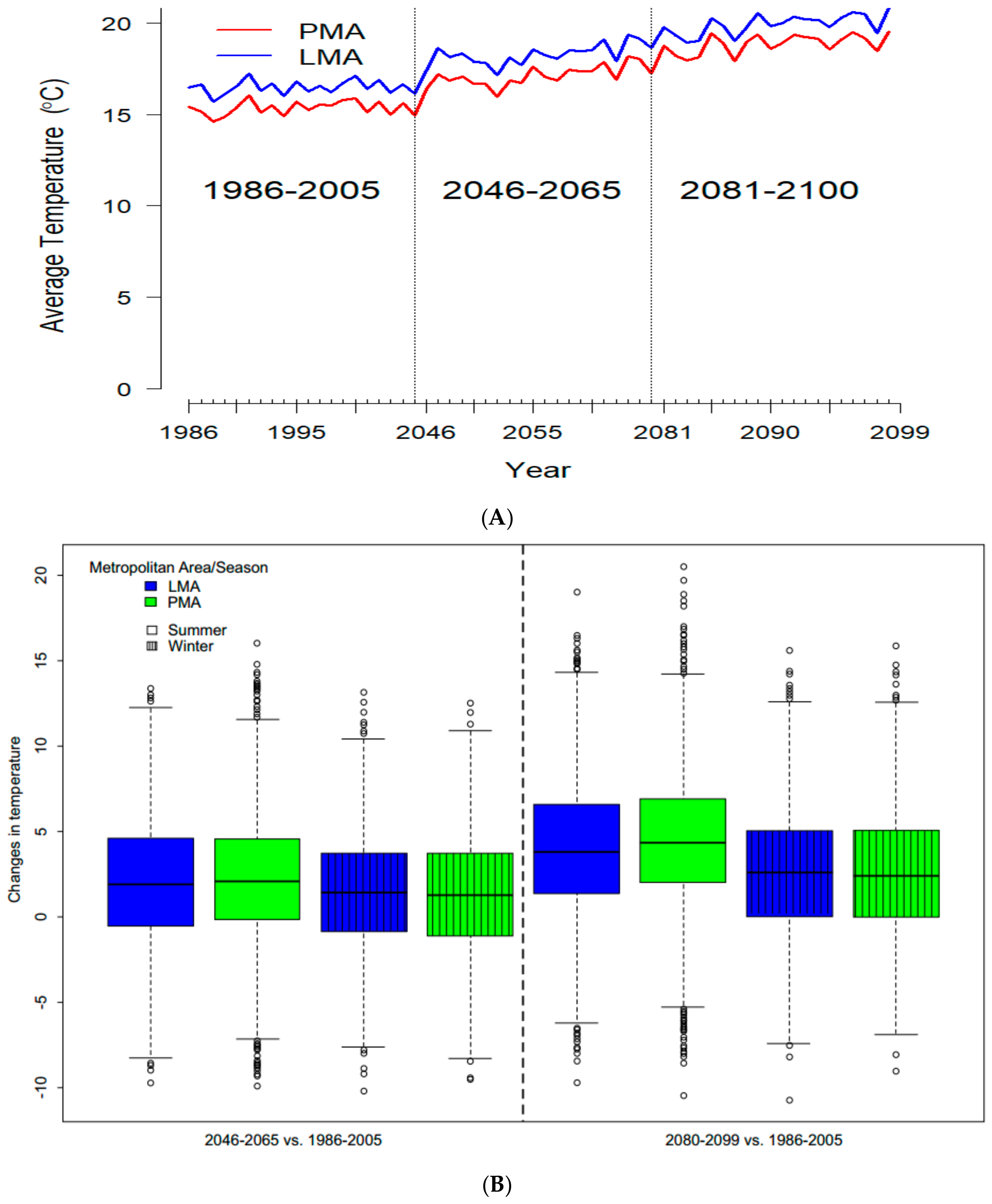
A total of 310,244 deaths (100,280 in PMA, Porto metropolitan area; and 209,964 in LMA, Lisbon metropolitan area) were recorded from 1986 to 2005, with more deaths in the winter than in the summer in both metropolitan areas (Table 1). The descriptive summaries of temperatures for the historical period 1986–2005 and the two future periods, 2046–2065 and 2080–2099, are presented in Table 1. The term “temperature” henceforth refers to daily minimum and maximum temperatures for winter and summer months, respectively, and daily mean temperature to the other months of the year. There is a general increase in average temperatures in both metropolitan areas for 2046–2065 and 2080–2099 (Table 1, Figure 2). For the historical period 1986–2005, the overall median daily temperature is 15.4 °C (Inter quarter range (IQR): 11.43–21.3 °C) for Lisbon and 14.5 °C (IQR: 10.0–26.0 °C) for PMA. Similarly, the median daily temperature in summer is 23.3 °C (IQR: 21.1–26.4 °C) for Lisbon and 23.1 °C (IQR: 21.2–26.0 °C) for Porto, while the median daily temperature is 9.8 °C (IQR: 7.6–11.9 °C) and 7.8 °C (IQR: 4.7–10.4 °C) for LMA and PMA, respectively.
The summer/winter temperature is projected to rise in the two metropolitan areas from the historical period to the end of the 21st century (Figure 2). This implies that temperatures in both metropolitan areas will become hotter. An increase in daily mean temperature is projected in the mid-term (2046–2065 vs. 1986–2005) for both summer and winter periods in both metropolitan areas. For example, the average projected increase in summer is 2.24 °C (IQR: −0.1 °C–4.6 °C) in PMA and 2.10 °C (IQR: −0.54 °C–4.66 °C) in LMA. Similarly, during the winter months, the average mean temperature increases in both metropolitan areas: 1.44 °C and 1.31 °C in PMA and LMA, respectively. A further increase in temperature was observed in the long-term projections (2065–2099 vs. 1986–2005). PMA exhibits a substantial increase in summer and winter temperatures, (4.51 °C, IQR: 2.02 °C −6.91 °C) and (2.52 °C, IQR: −0.03 °C–5.04 °C), respectively, higher than LMA, (4.01 °C, IQR: 1.40 °C–6.60 °C) and (2.71 °C, IQR: 0.10 °C–5.10 °C), for summer and winter, respectively.

3.1. Historical Association between Temperature and Mortality

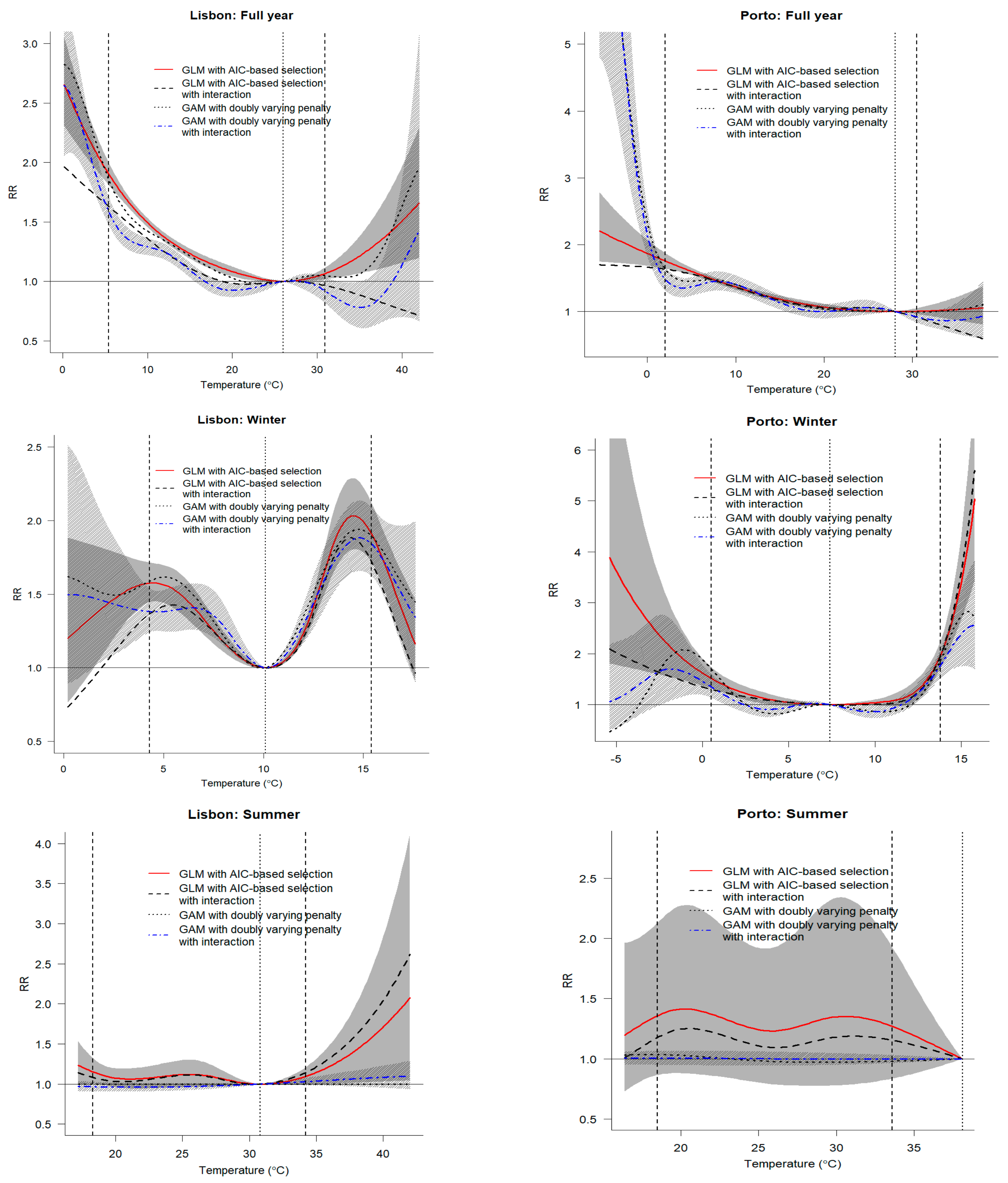
In the first instance, temperature–mortality was based on four modelling formulations: GLM with AIC-based selection, GLM with AIC-based selection with interaction, GAM with double varying penalty, and GAM with double varying penalty with interaction. The reference temperature for the preliminary analysis was the MMT, estimated from the GLM with AIC-based selection model (dashed lines in Figure 3). The estimated cumulative associations displaying the relationship between daily temperature and mortality (1986–2005) in LMA and PMA for the whole year, summer, and winter (over the entire lag period of 0–30 days) are presented in Figure 3.
The results obtained from four models on temperature–mortality association are displayed in Figure 3, Figure 4 and Figures S1–S3 for the whole year, winter, and summer months for the historical period. The models are based on MMT derived from GLM with AIC-based selection criteria for LMA and PMA, respectively. Figure 3 shows that the temperature–mortality curves for LMA are broadly U-shaped with significantly higher risk of mortality at lower temperatures, except for GLM with AIC-based selection model with interaction. A similar pattern-inverted J-shaped of the exposure–response curve was observed in PMA for all models, except GLM with AIC-based selection model with interaction.
Regarding winter months, the temperature–response curves were w-shaped with two peaks for LMA, while those of PMA were either u-shaped or w-shaped. The temperature–mortality association in the summer months is generally non-significant in both metropolitan areas, except in LMA at high temperatures using GLM with AIC-based selection with/without interaction. In general, the nonlinear exposure–response shows higher risk at lower temperatures than at high temperatures.
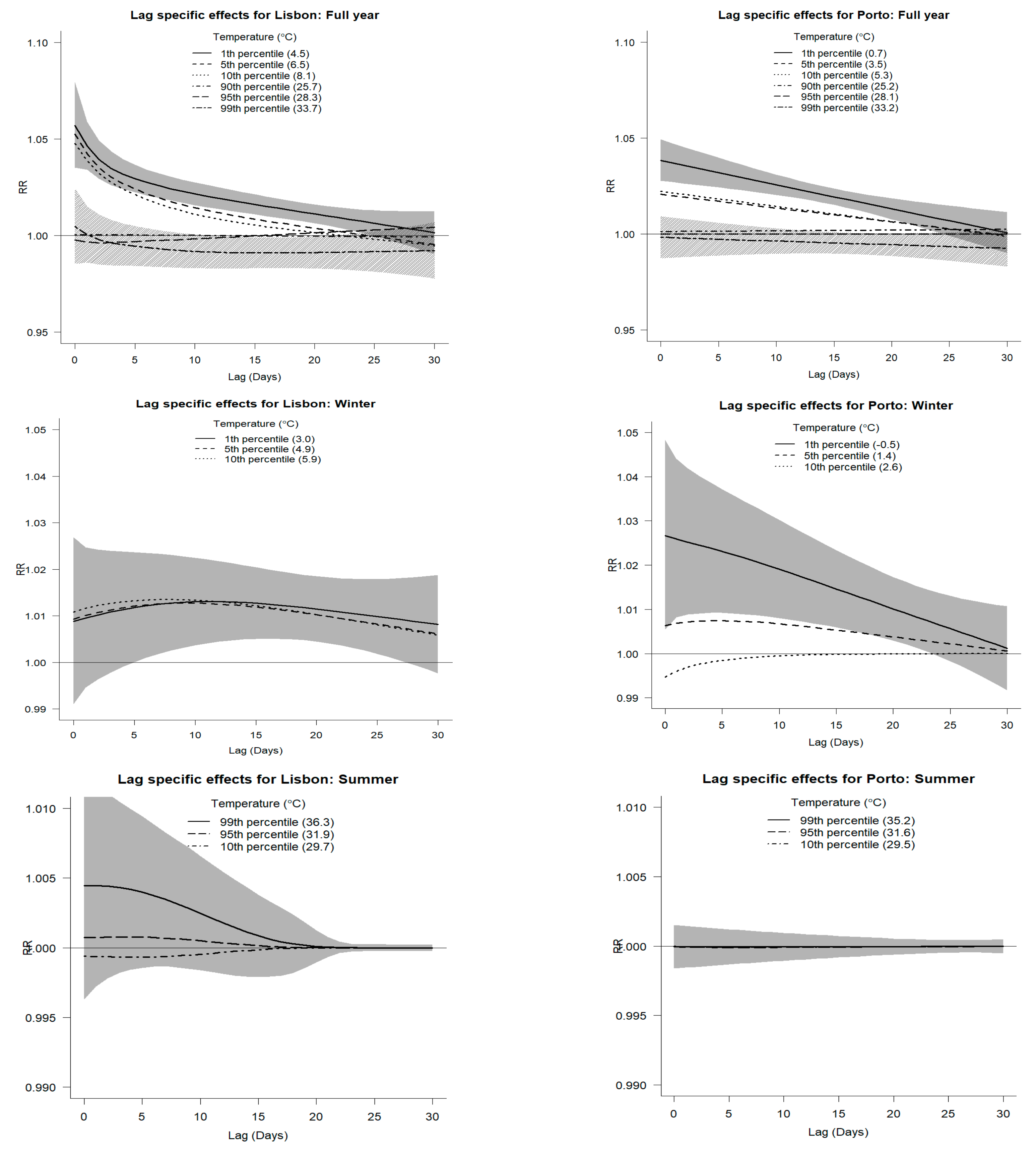
The lag-specific effect of temperature–mortality relationship over lags of 0–30 days is presented in Figure 4. We observed immediate effects of both cold and hot temperatures on mortality for the whole year in LMA; however, in PMA, we only observed cold effects. The cold effect in the winter months in LMA is delayed for about 5 days (middle panel, Figure 4). The cold effect in PMA is strong and statistically significant for up to 23 days.
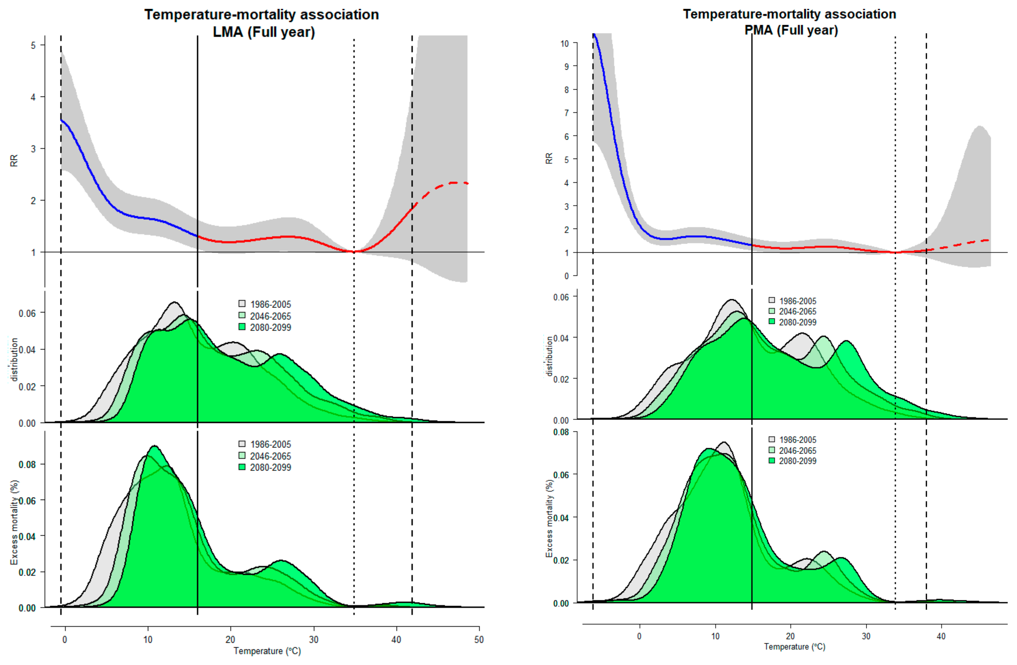
A further and detailed investigation of exposure–lag–response association will be based on GAM with a double varying penalties model with interaction due to its precise estimates (Figure 5, Figure 6 and Figure 7, Tables S1 and S2). The MMTs for LMA for the whole year, summer and winter months are 35.1 °C (95% CI: 21.3–42.0 °C), 21.6 °C (95% CI: 17.1–42.0 °C), and 10.1 °C (95% CI: 0.2–17.7 °C), respectively. Similarly, the MMT for PMA corresponds to 34.1 °C (95% CI: 29.5–38.1 °C) for the whole year, 31.5 °C (95% CI: 16.3–38.1 °C) for summer months, and 9.8 °C (95% CI: −5.5–10.4 °C) for winter months. The longer widths of the confidence reflect the uncertainty around the MMT.
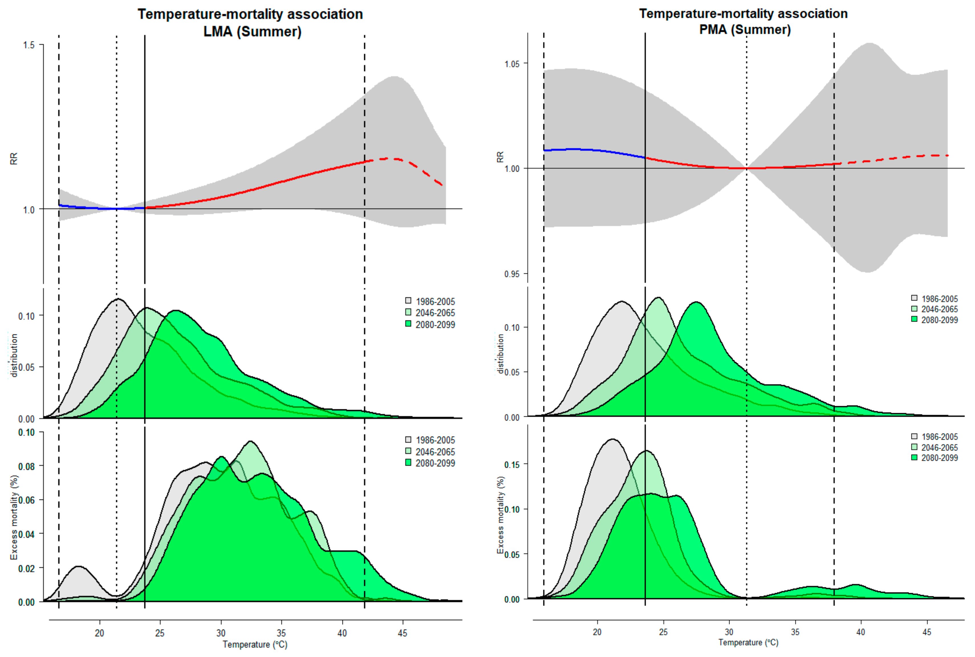
The total cumulative exposure–response for the whole year, showing the mortality risk associated with temperature, is summarized in the top panel of Figure 5 and Table 2. The overall cumulative risk for mortality due to temperature generally indicates an increased risk at lower temperatures in both metropolitan areas. For example, the RRs at the 1st vs. the 99th temperature percentiles in LMA (4.5 °C vs. 33.7 °C) and PMA (0.7 °C vs. 33.3 °C) are 2.30 (95% CI: 1.84–2.88) vs. 1.03 (95% CI: 0.96–1.09) and 2.07 (95% CI: 1.66–2.58) vs. 1.00 (95% CI: 0.95–1.06), respectively. However, during the winter period, the temperature–mortality relationship suggests a significant mortality risk associated with both cold and warmer temperature (except the mean) (Figure 6, top panel, and Table 2) in both metropolitan areas. Though significant increases in RRs were observed in LMA from 4 °C–6 °C to 11 °C–16 °C (top right panel of Figure 6), the RR reached its peak at 14.5 °C (RR = 1.36, 95% CI: 1.19–1.54), which is higher than the 1st percentile, 3.0 °C (RR = 1.45, 95% CI: 1.16–1.82). The temperature-associated RR for PMA in winter at the 1st temperature percentile (−0.5 °C) was 1.82 (95% CI: 1.41, 2.34), peaking at 15.5 °C with a RR of 3.52 (95% CI: 2.29, 5.39). During the summer months, the associated risks due to 30 days of cumulative exposure were non-significant. For example, the RRs associated with the 99th temperature percentile, 36.3 °C in LMA and 35.2 °C in PMA, were 1.09 (95% CI: 1.00, 1.19) and 1.00 (95% CI: 0.98, 1.02), respectively (Figure 7 and Table 2).
The attributable mortality fractions (for the historical period), estimated for the combined and separate effects of cold and hot temperatures, are presented in Table 2 and Table S1. The overall attributable mortality fraction (caused by hot and cold temperature) for the whole year in LMA is 30.21% (95% eCI: 12.63–42.62) and it is mostly due to cold temperature: 30.16% (95% eCI: 15.56–42.58) (Table S1). Our results also show that, in PMA, a high proportion of temperature-attributable fractions is due to cold (RR = 22.83, 95% eCI: 13.72–30.92), with a total attributable fraction of 22.26 (95% eCI: 12.77–41.98). The total fraction of deaths attributed to varying temperatures is predominantly due to cold and it is higher in winter (3.18% in LMA vs. 5.37% in PMA) than in summer (0.36% in LMA vs. 0.18% in PMA). The attributable fraction of deaths due to hot temperature is generally non-significant (Table S1).

3.2. Projected Temperature-Related Mortality Rates

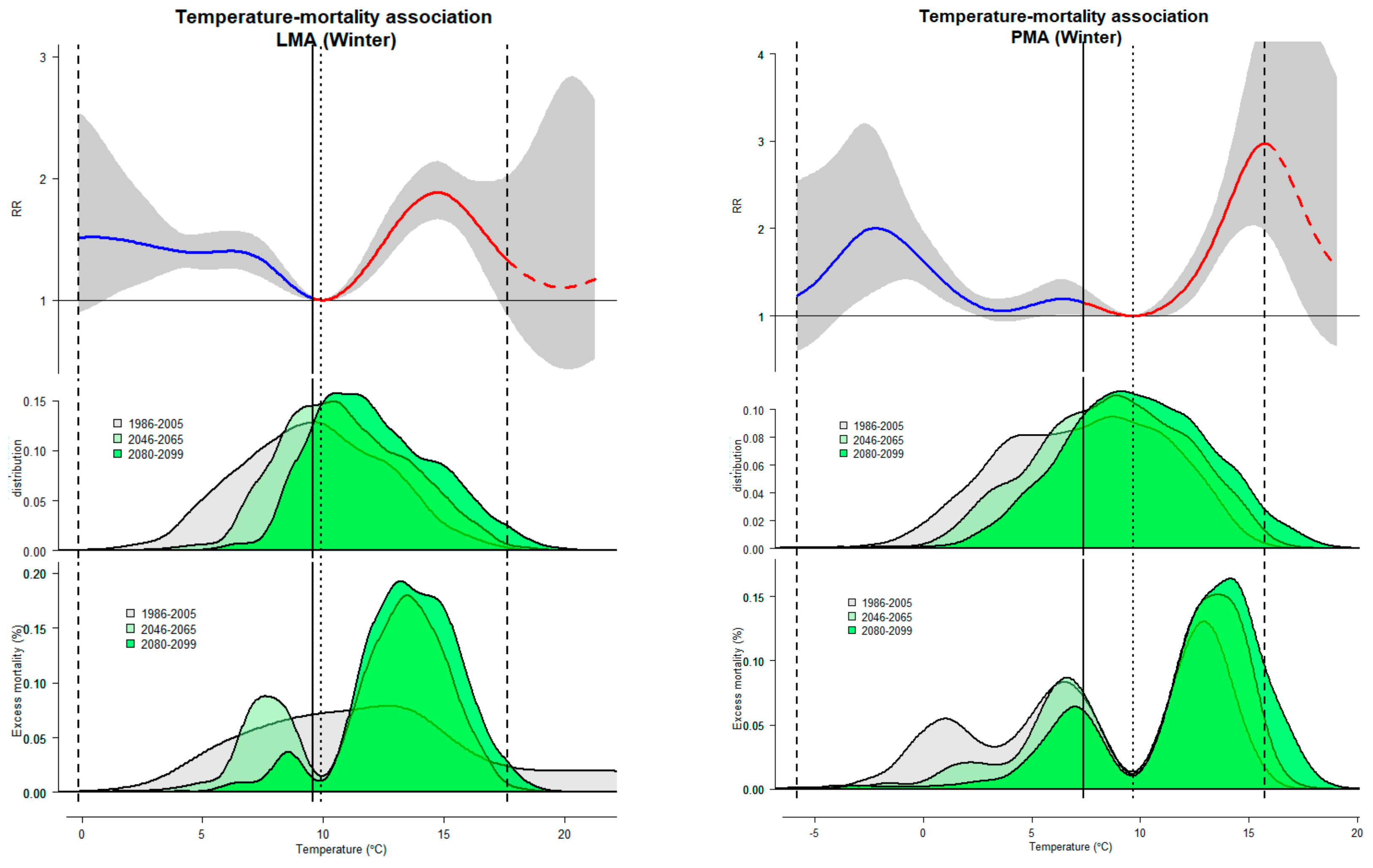
Using projected patterns of mortality based on average daily counts of the year from the historical data (1986–2005), we present the RR across the temperature (°C) range, with 95% empirical confidence intervals extrapolated beyond the maximum temperature during the historical period (Top panel, Figure 5, Figure 6 and Figure 7). The variation in daily temperature and estimated attributable mortality are displayed in Figure 5, Figure 6 and Figure 7 (middle and bottom panel). In general, in Figure 5, Figure 6 and Figure 7, we can observe that the mortality burden due to cold temperatures is much higher in the historical period (1986–2005) than the hot-related burden in both metropolitan areas for the whole year, summer, and winter periods. The proportion attributable to cold temperature decreases over the future periods. On the contrary, the hot-related burden is relatively higher in the future periods than in the current period.
The projected overall attributable fractions of temperature-related (cold and hot) in both metropolitan areas are summarized in Table S1 and S2. Our findings show a slight decrease in the total temperature-related mortality, considering the entire future years in both metropolitan areas. Our results project a total decrease from 30.21% (95% eCI: 12.63–42.62) for the historical period to 27.67% (95% eCI: 9.82–40.41) and 26.01% (95% eCI: 7.82–38.84) in the 2046–2065 and 2081–2099 periods, respectively, in LMA (Table S1). Similar results were found in PMA for the whole year, with decreases from 28.26% (95% eCI: 12.77–41.98) in the 1986–2005 period to 26.32% (95% eCI: 10.82–40.06) and 24.38% (95% eCI: 9.08–38.02) in the 2046–2065 and 2081–2099 periods, respectively.
The projected changes in excess hot-, cold-, and temperature-related mortality rates in LMA and PMA in the mid-term (2046–2065) and long-term (2080–2099), compared to the historical period (1986–2005), are presented in Table S2. Our results reveal varying excess mortality attributable to temperature. Compared to the historical period, there is a general significant decrease in the estimated proportion of temperature-attributable deaths in both metropolitan areas over the future periods (Table S2), except in the winter. There is a net reduction of −2.53% and −4.20% in temperature-related excess mortality for the 2046–2065 and 2081–2099 periods (whole year) compared to the historical period 1986–2005 (Table S2). However, we found an increase in cold-related excess mortality from 1.44% (95% CI: 1.15–1.66) in 2046–2065 to 3.14% (95% CI: 2.25–3.76) during 2081–2099 in LMA. The opposite was observed in PMA during the winter, as there was a decrease in cold-related excess mortality from −0.71% (95% CI: −1.27–−0.04) in 2046–2065 to −1.23% (95% CI: −2.18–−0.08). Interestingly, the excess mortality attributable to hot temperatures is not significant in the two metropolitan areas throughout the future periods.
Considering the changes in mortality due to temperature in the future years, we should first note that the winter season is becoming warmer over the century. For example, the 1st temperature percentile in the historical (1986–2005) and future periods (2045–2065 and 2081–2099) are 3.0 °C, 5.5 °C, and 7.1 °C in LMA and −0.5 °C, 1.3 °C, and 2.8 °C in PMA, respectively. In the same vein, the mortality due to extreme cold also declines over the century, while an increase in the attributable risk with warmer winter temperatures was observed. There is a significant decreasing trend in proportion to the overall extreme cold temperature-attributable mortality in LMA in the future periods (2045–2065 and 2081–2099), compared to the historical period (−0.63%, 95% eCI: −0.7%, −0.52%) and (−0.73%, 95% eCI: −0.81%, −0.61%), respectively. Similar results were observed in PMA (−0.62%, 95% eCI: −0.70, –0.52) for 2045–2065 and (−0.69%, 95% eCI: −0.78, −0.58) for 2081–2099, compared to the historical period. The attributable fraction due to extreme hot temperature in the summer months increased by 0.08% and 0.23%, from 0.04% (95% eCI: 0.00%, 0.07%) in the historical period to 0.11% (95% eCI: −0.01%, 0.22%) during 2046–2065, and to 0.27% (95% eCI: −0.02%, 0.54%) during 2081–2099 in LMA. While there were no noticeable changes due to extreme hot temperature during the summer in PMA, significant increases were observed in warmer winter temperatures, 1.27% (0.88%, 1.52%) and 2.80% (1.63%, 3.44%), respectively.
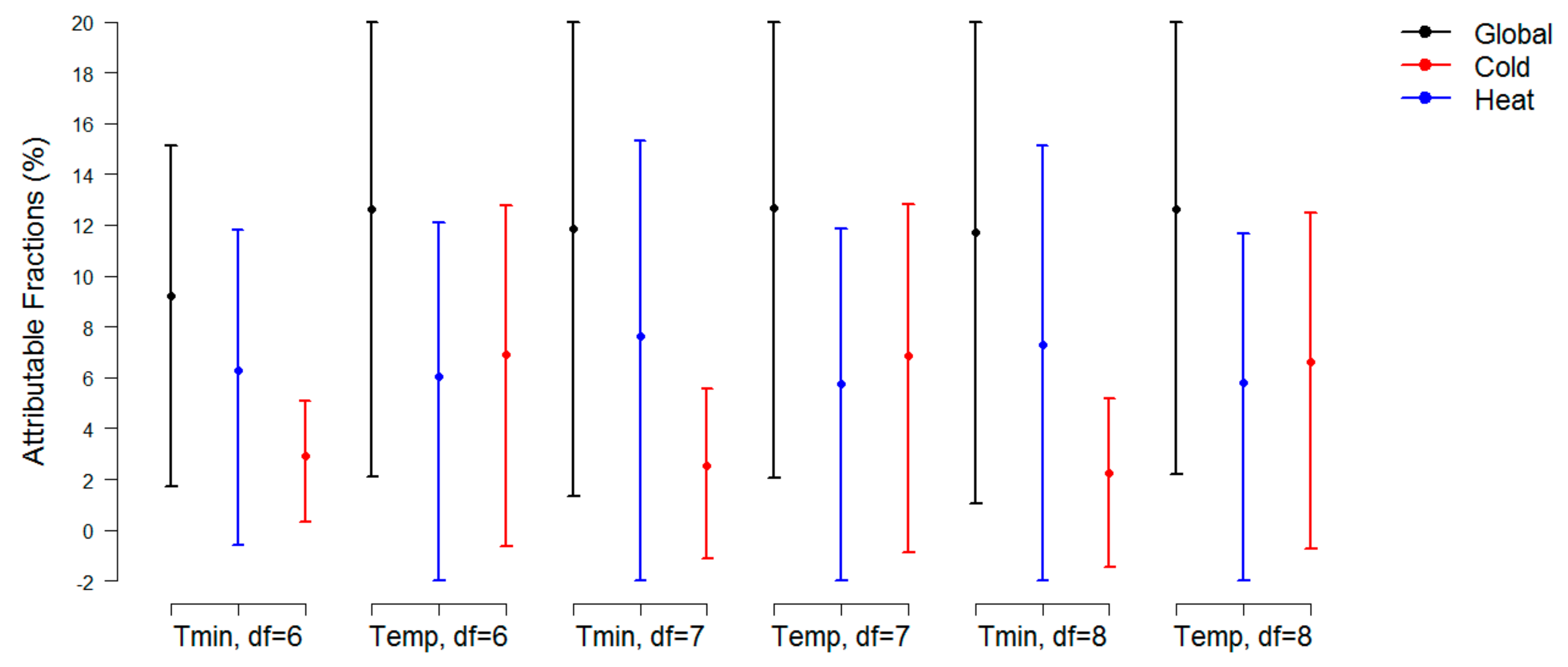
We carried out a sensitivity analysis to evaluate the choice of functional relationships for temperature-mortality and lag-mortality, and we explored constant, linear, and quadratic B-splines for exposure–lag–response functional relationships using different temperature variables (minimum, mean, and maximum), and degrees of freedom (6–8 per year). As shown in Figure 8, the effects of using different dfs, as well as minimum temperatures on attributable fractions are minimal.

4. Discussion

In this study, we investigated the impact of temperature on CSD mortality in two metropolitan areas (LMA and PMA) in Portugal, using DLNM with a quasi-Poisson family. This was performed for the late 20th and 21st centuries (historical past: 1986–2005; mid-term: 2046–2065; and long-term: 2080–2099). The average, minimum, and maximum daily temperatures were obtained for the present reference (historical period), mid- and long-term climates via regional model simulations using the Weather Research and Forecasting (WRF) model forced by the MPI-ESM-LR model. To the best of our knowledge, this is the first study to project temperature-related excess mortality due to CSD using future daily temperatures simulated by a regional model.
Our results showed that changes in average temperature in both metropolitan areas are projected to increase over the 21st century. We found that changes in temperature-related mortality from diseases of the circulatory system vary with geographical location and season.
The increase in projected temperatures and its adverse effects observed in this study are not surprising, as climate change has been reported to be a dominant driver of the projected weather-related hazards trend, accounting for more than 90% of the rise in the risk to human beings [37]. It is clear from epidemiological studies that the effects of weather-related hazards on human lives differ greatly in terms of both magnitude and rate of change, and that heatwaves are the most lethal weather-related hazard [37]. A multi-country global study projected temperature-related mortality risks at the end of the century in over 400 locations, for several climate change scenarios [1]. The study reported that areas with hotter climates, such as Central and South America, Southern Europe, and Southeast Asia, exhibit an increased impact of climate change [1]. These regions are currently characterized by relatively higher heat-related impacts, which are projected to rise considerably by the end of the century under the RCP8.5, reaching 10.5% (95% eCI: 5.6 to 17.3) in Southern Europe and 16.7% (−1.7 to 33.2) in Southeast Asia [1].
The LMA findings are consistent with similar US studies that have shown an increase in summer temperature-related mortality and a decreased risk associated with winter temperatures, under several climate change scenarios [38]. The same results for PMA in winter months. Similarly, a European study [2] reported that the rise in heat-related mortality will start to completely compensate for the reduction of deaths from cold during the period from 2070 to 2100 [2]. Weinberger et al. [38] also showed that rates of heat-related deaths will increase in 10 US metropolitan areas in 2050, compared with 1997, with a further increase in 2090.
Some studies suggest that the effects of extreme temperatures can be reduced when preventive measures are implemented [39,40,41]. According to a study in Spain [40], provinces that implemented more actions from their Heat Health Prevention Plan showed stronger decreases in mortality attributable to extreme heat. Evidence from Montreal, Canada, suggests that the heat action plan implemented in 2004 reduced mortality overall on hot days between 2004 and 2007 [41]. Weinberger et al. [38] found that the US National Weather Service heat alerts were not associated with lower mortality in most cities studied, potentially missing a valuable opportunity to avert a substantial number of heat-related deaths.
Some limitations in this study must be acknowledged. Firstly, we did not account for changes in the population or its composition, because that may result in an underestimate of the health impact of climate change [3,42]. Secondly, mortality projections were based on the average number of deaths in the historical period projected into the future. This conservative approach may underestimate the temperature-related mortality in these metropolitan areas. Thirdly, though temperature variability may also influence air quality, in this study, we did not investigate the effects of air quality. Lastly, as discussed in Gasparrini et al. [43], the smoothing methods for exposure–lag–response relationships are difficult to validate in DLNM. Nonetheless, the assumptions made in this study are reasonable in the absence of adequate information and the importance of our findings is not reduced. This research provides a detailed assessment of cold and hot temperature–mortality risks in Lisbon and Porto metropolitan areas, in both current and projected time periods. we did not consider changes.

5. Conclusions

In Portugal, the Directorate-General of Health (DGS) has designed Contingency Plans for Heatwaves [8,44] and Cold Weather [45] that provide information and advice so as to minimize the risk of exposure to extreme temperatures. However, this is not sufficient. The goal of a national health adaptation strategy or plan should be to build the resilience of the existing health system [34,46,47,48,49]. The lack of a broad climate monitoring network has been a substantial obstacle to the creation of local climate adaptation plans to real and credible climate changes. This also prevents a thorough and accurate dissemination of population warnings on the occurrence of extreme weather events for entire regions. In the future, these plans must integrate the temperature projections from regional climate models (RCM) and combine them with the current or potential empirical exposure– response relationship and related vulnerabilities for each metropolitan area.

Supplementary Materials

The following are available online at https://www.mdpi.com/2073-4433/10/12/735/s1, Figure S1: Individual overall cumulative exposure-response curve: LMA (Lisbon metropolitan area)—Full year (Top) and Porto metropolitan area (PMA)—Full year (Bottom), Figure S2: Individual overall cumulative exposure-response curve: LMA (Lisbon metropolitan area)—WINTER (Top) and PMA (Porto metropolitan area)—WINTER (Bottom), Figure S3: Individual overall cumulative exposure-response curve: LMA (Lisbon metropolitan area)—SUMMER (Top) and PMA (Porto metropolitan area)—SUMMER (Bottom), Table S1: Attributable mortality (%) with 95% empirical confidence interval evaluated for the recent past (1986–2005)—using minimum mortality temperature (MMT) as a reference—for Lisbon and Porto metropolitan areas—Portugal, Table S2: Excess mortality attributable to temperature in the future periods (2046-2065) and (2080-2099) relative to the historical period (1986-2005), together with their 95% empirical confidence interval.

Author Contributions

Conceptualization, M.R., P.S., and A.R.; Methodology, M.R., P.S. and A.R.; Software, M.R. and A.R.; Writing—original draft preparation, M.R.; Writing—review and editing, M.R., P.S. and A.R.

Funding

This study was partially supported by the European Regional Development Funds, through the COMPETE 2020—Operational Programme “Competitiveness and Internationalization,” under Grant POCI-01-0145-FEDER-006891; and by National Funds through the Portuguese Foundation for Science and Technology (FCT) under Grant UID/GEO/04084/2013. The authors wish to thank the financial support to CESAM (UID/AMB/50017/2019) to FCT/MEC through national funds and the co-funding by the FEDER within the PT2020 Partnership Agreement and Compete 2020.

Acknowledgments

The authors would like to thank the Portuguese National Statistics Institute—Statistics Portugal for its support with obtaining the health data from this database.

Conflicts of Interest

The authors declare no conflict of interest. The funders had no role in the design of the study; in the data collection, data analysis, or interpretation of data; in the writing of the manuscript, or in the decision to publish the results. The corresponding author had full access to all the data in the study.

References

  1. Gasparrini, A.; Guo, Y.; Sera, F.; Vicedo-Cabrera, A.M.; Huber, V.; Tong, S.; Coelho, M.S.Z.S.; Saldiva, P.H.N.; Lavigne, E. Projections of temperature-related excess mortality under climate change scenarios. Lancet Planet Health 2017, 1, e360–e367. [Google Scholar] [CrossRef]
  2. Ballester, J.; Robine, J.M.; Hermann, F.; Rodó, X. Long-term projections and acclimatization scenarios of temperature-related mortality in Europe. Nat. Commun. 2011, 2, 358. [Google Scholar] [CrossRef]
  3. Petkova, E.; Horton, R.; Bader, D.; Kinney, P. Projected Heat-Related Mortality in the U.S. Urban Northeast. Int. J. Environ. Res. Public Health 2013, 10, 6734–6747. [Google Scholar] [CrossRef]
  4. Díaz, J.; López-Bueno, J.A.; Sáez, M.; Mirón, I.J.; Luna, M.Y.; Sánchez-Martínez, G.; Carmona, R.; Barceló, M.A.; Linares, C. Will there be cold-related mortality in Spain over the 2021–2050 and 2051–2100 time horizons despite the increase in temperatures as a consequence of climate change? Environ. Res. 2019, 176, 108557. [Google Scholar] [CrossRef]
  5. Almendra, R.; Santana, P.; Mitsakou, C.; Heaviside, C.; Samoli, E.; Rodopoulou, S.; Vardoulakis, S. Cold-related mortality in three European metropolitan areas: Athens, Lisbon and London. Implications for health promotion. Urban Clim. 2019, 30, 100532. [Google Scholar] [CrossRef]
  6. Vicedo-Cabrera, A.M.; Sera, F.; Gasparrini, A. Hands-on Tutorial on a Modeling Framework for 482 Projections of Climate Change Impacts on Health. Epidemiology 2019, 30, 321–329. [Google Scholar] [CrossRef]
  7. Rodrigues, M.; Santana, P.; Rocha, A. Effects of extreme temperatures on cerebrovascular mortality in Lisbon: A distributed lag non-linear model. Int. J. Biometerol. 2019, 63, 549–559. [Google Scholar] [CrossRef]
  8. Casanueva, A.; Burgstall, A.; Kotlarski, S.; Messeri, A.; Morabito, M.; Flouris, A.D.; Nybo, L.; Spirig, C.; Schwierz, C. Overview of Existing Heat-Health Warning Systems in Europe. Int. J. Environ. Res. Public Health 2019, 16, 2657. [Google Scholar] [CrossRef]
  9. Morabito, M.; Crisci, A.; Moriondo, M.; Profili, F.; Francesconi, P.; Trombi, G.; Bindi, M.; Gensini, G.F.; Orlandini, S. Air temperature-related human health outcomes: Current impact and estimations of future risks in Central Italy. Sci. Total Environ. 2012, 441, 28–40. [Google Scholar] [CrossRef]
  10. Ravindra, K.; Rattan, P.; Mor, S.; Aggarwal, A. Generalized additive models: Building evidence of air pollution, climate change and human health. Environ. Int. 2019, 132, 104987. [Google Scholar] [CrossRef]
  11. Kakkoura, M.; Kouis, P.; Papatheodorou, S.I.; Paschalidou, A.K.; Ziogas, K. The effect of ambient temperature on cardiovascular and respiratory mortality in Thessaloniki, Greece. Sci. Total. Environ. 2018, 647, 1351–1358. [Google Scholar]
  12. Martínez, G.S.; Díaz, J.; Hooyberghs, H.; Lauwaet, D.; De Ridder, K.; Linares, C.; Carmona, R.; Ortiz, C.; Kendrovski, V.; Aerts, R.; et al. Heat and health under climate change in Antwerp: Projected impacts and implications for prevention. Environ. Int. 2018, 111, 135–143. [Google Scholar] [CrossRef] [PubMed]
  13. Gasparrini, A. Distributed lag linear and non-linear models in R: The package dlnm. J. Stat. Softw. 2011, 43, 1–20. [Google Scholar] [CrossRef] [PubMed]
  14. Neophytou, A.M.; Picciotto, S.; Brown, D.M.; Gallagher, L.E.; Checkoway, H.; Eisen, E.A.; Costello, S. Exposure-lag-response in longitudinal studies: Application of distributed lag non-linear models in an occupational cohort. Am. J. Epidemiol. 2018, 187, 1539–1548. [Google Scholar] [CrossRef] [PubMed]
  15. Hajat, S.; Vardoulakis, S.; Heaviside, C.; Eggen, B. Climate change effects on human health: Projections of temperature-related mortality for the UK during the 2020s, 2050s and 2080s. J. Epidemiol. Community Health 2014, 68, 641–648. [Google Scholar] [CrossRef]
  16. Baaghideh, M.; Mayvaneh, F. Climate Change and Simulation of Cardiovascular Disease Mortality: A Case Study of Mashhad, Iran. Iran J. Public Health 2017, 46, 396–407. [Google Scholar]
  17. Giang, P.N.; Dung, D.V.; Giang, K.B.; Vinhc, H.V.; Rocklöv, J. The effect of temperature on cardiovascular disease hospital admissions among elderly people in Thai Nguyen Province, Vietnam. Glob. Health Action 2014, 7, 23649. [Google Scholar] [CrossRef]
  18. Messner, T. Environmental variables and the risk of disease. Int. J. Circumpolar Health 2005, 64, 523–533. [Google Scholar] [CrossRef]
  19. Nocera, R.; Petrucelli, P.; Park, J.; Stander, E. Meteorological Variables Associated with Stroke. Int. Sch. Res. Not. 2014, 2014, 597106. [Google Scholar] [CrossRef]
  20. Li, T.; Horton, R.M.; Kinney, P. Future projections of seasonal patterns in temperature-related deaths for Manhattan, New York. Nat. Clim. Chang. 2013, 3, 717–721. [Google Scholar] [CrossRef]
  21. Baccini, M.; Kosatsky, T.; Analitis, A.; Anderson, H.R.; D’Ovidio, M.; Menne, B.; Michelozzi, P.; Biggeri, A.; PHEWE Collaborative Group. Impact of heat on mortality in 15 European cities: Attributable deaths under different weather scenarios. J. Epidemiol. Community Health 2011, 65, 64–70. [Google Scholar] [CrossRef] [PubMed]
  22. Kinney, P.L. Temporal Trends in Heat-Related Mortality: Implications for Future Projections. Atmosphere 2018, 9, 409. [Google Scholar] [CrossRef]
  23. Scovronick, N.; Sera, F.; Acquaotta, F.; Garzena, D.; Fratianni, S.; Wright, C.Y.; Gasparrini, A. The association between ambient temperature and mortality in South Africa: A time-series analysis. Environ. Res. 2018, 161, 229–235. [Google Scholar] [CrossRef] [PubMed]
  24. Achebak, H.; Devolder, D.; Ballester, J. Trends in temperature-related age-specific and sex-specific mortality from cardiovascular diseases in Spain: A national time-series analysis. Lancet Planet. Heal. 2019, 3, e297–e306. [Google Scholar] [CrossRef]
  25. Moss, R.; Babiker, M.; Brinkman, S.; Calvo, E.; Carter, T.; Edmonds, J.; Elgizouli, I.; Emori, S.; Erda, L.; Hibbard, K.; et al. Towards New Scenarios for Analysis of Emissions, Climate Change, Impacts, and Response Strategies; Intergovernmental Panel on Climate Change: Geneva, Switzerland, 2008. [Google Scholar]
  26. Moss, R.H.; Edmonds, J.A.; Hibbard, K.A.; Manning, M.R.; Rose, S.K.; Van Vuuren, D.P.; Carter, T.R.; Emori, S.; Kainuma, M.; Meehl, G.A.; et al. The next generation of scenarios for climate change research and assessment. Nature 2010, 463, 747. [Google Scholar] [CrossRef] [PubMed]
  27. Riahi, K.; Rao, S.; Krey, V.; Cho, C.; Chirkov, V.; Fischer, G.; Kindermann, G.; Nakicenovic, N.; Rafaj, P. RCP 8.5 - A scenario of comparatively high greenhouse gas emissions. Clim. Chang. 2011, 109, 33. [Google Scholar] [CrossRef]
  28. Intergovernmental Panel on Climate Change (IPCC). The Physical Science Basis. Contribution of Working Group I to the Fifth Assessment Report of the Intergovernmental Panel on Climate Change; Cambridge University Press: Cambridge, NY, USA, 2013; p. 1535. [Google Scholar]
  29. Giorgetta, M.A.; Jungclaus, J.; Reick, C.H.; Legutke, S.; Bader, J.; Bottinger, M.; Brovkin, V.; Crueger, T.; Esch, M.; Fieg, K. Climate and carbon cycle changes from 1850 to 2100 in MPI-ESM simulations for the Coupled Model Intercomparison Project phase 5. J. Adv. Model. Earth Syst. 2013, 5, 572–597. [Google Scholar] [CrossRef]
  30. Marta-Almeida, M.; Teixeira, J.C.; Carvalho, M.J.; Melo-Gonçalves, P.; Rocha, A.M. High resolution WRF climatic simulations for the Iberian Peninsula: Model validation. Phys. Chem. Earth 2016, 94, 94–105. [Google Scholar] [CrossRef]
  31. Viceto, C.; Cardoso Pereira, S.; Rocha, A. Climate Change Projections of Extreme Temperatures for the Iberian Peninsula. Atmosphere 2019, 10, 229. [Google Scholar] [CrossRef]
  32. Fonseca, D.; Carvalho, M.J.; Marta-Almeida, M.; Melo-Gonçalves, P.; Rocha, A. Recent trends of extreme temperature indices for the Iberian Peninsula. Phys. Chem. Earth 2016, 94, 66–76. [Google Scholar] [CrossRef]
  33. Pereira, S.C.; Marta-Almeida, M.; Carvalho, A.C.; Rocha, A. Heat wave and cold spell changes in Iberia for a future climate scenario. Int. J. Climatol. 2017, 37, 5192–5205. [Google Scholar] [CrossRef]
  34. Rodrigues, M.; Santana, P.; Rocha, A. Bootstrap approach to validate the performance of models for predicting mortality risk temperature in Portuguese metropolitan areas. Environ. Health 2019, 18, 25. [Google Scholar] [CrossRef] [PubMed]
  35. Gasparrini, A.; Leone, M. Attributable risk from distributed lag models. BMC Med. Res. Methodol. 2014, 14, 55. [Google Scholar] [CrossRef] [PubMed] [Green Version]
  36. Gasparrini, A.; Guo, Y.; Hashizume, M.; Lavigne, E.; Zanobetti, A.; Schwartz, J.; Tobias, A.; Tong, S.; Rocklöv, J.; Forsberg, B.; et al. Mortality risk attributable to high and low ambient temperature: A multicountry observational study. Lancet 2015, 386, 369–375. [Google Scholar] [CrossRef]
  37. Forzieri, G.; Cescatti, A.; Silva, F.B.; Feyen, L. Increasing risk over time of weather-related hazards to the European population: A data-driven prognostic study. Lancet Planet Health 2017, 1, e200–e208. [Google Scholar] [CrossRef]
  38. Weinberger, K.R.; Haykin, L.; Eliot, M.N.; Schwartz, J.D.; Gasparrini, A.; Wellenius, G.A. Projected temperature-related deaths in ten large US metropolitan areas under different climate change scenarios. Environ. Int. 2017, 107, 196–204. [Google Scholar] [CrossRef]
  39. Guo, Y.; Barnett, A.G.; Tong, S. High temperatures-related elderly mortality varied greatly from year to year: Important information for heat-warning systems. Sci. Rep. 2012, 2, 830. [Google Scholar] [CrossRef] [Green Version]
  40. Martínez-Solanas, E.; Basagaña, X. Temporal changes in temperature-related mortality in Spain and effect of the implementation of a Heat Health Prevention Plan. Environ. Res. 2018, 169, 102–113. [Google Scholar] [CrossRef]
  41. Benmarhnia, T.; Bailey, Z.; Kaiser, D.; Auger, N.; King, N.; Kaufman, J.S. A difference-in-differences approach to assess the effect of a heat action plan on heat-related mortality, and differences in effectiveness according to sex, age, and socioeconomic status (Montreal, Quebec). Environ. Health Perspect. 2016, 124, 1694–1699. [Google Scholar] [CrossRef] [Green Version]
  42. Knowlton, K.; Lynn, B.; Goldberg, R.A.; Rosenzweig, C.; Hogrefe, C.; Rosenthal, J.K.; Kinney, P.L. Projecting heat-related mortality impacts under a changing climate in the New York City region. Am. J. Public Health 2007, 97, 2028–2034. [Google Scholar] [CrossRef]
  43. Gasparrini, A.; Scheipl, F.; Armstrong, B.; Kenward, M.G. A penalized framework for distributed lag non-linear models. Biometrics 2017, 73, 938–948. [Google Scholar] [CrossRef]
  44. DGS—Direção Geral de Saúde. Plano de Contingência para Temperaturas Extremas Adversas—Módulo de Calor 2014. Available online: https://www.dgs.pt/documentos-e-publicacoes/plano-de-contingencia-para-temperaturas-extremas-adversas-modulo-calor-2014.aspx (accessed on 18 September 2019).
  45. DGS—Direção Geral de Saúde. Plano de Contingência Para Temperaturas Extremas Adversas—Módulo Inverno 2016. Available online: https://www.dgs.pt/documentos-e-publicacoes/saude-sazonal-inverno-saude-.aspx (accessed on 18 September 2019).
  46. Watts, N.; Amann, M.; Arnell, N.; Ayeb-Karlsson, S.; Belesova, K.; Berry, H.; Bouley, T.; Boykoff, M.; Byass, P.; Cai, W.; et al. The 2018 report of the Lancet Countdown on health and climate change: Shaping the health of nations for centuries to come. Lancet 2018, 392, 2479–2514. [Google Scholar] [CrossRef]
  47. Martinez, G.S.; Linares, C.; Ayuso, A.; Kendrovski, V.; Boeckmann, M.; Diaz, J. Heat-health action plans in Europe: Challenges ahead and how to tackle them. Environ. Res. 2019, 176, 108548. [Google Scholar] [CrossRef]
  48. Sheridan, S.C.; Kalkstein, L.S. Progress in heat watch-warning system technology. Bull. Am. Meteorol. Soc. 2004, 85, 1931–1941. [Google Scholar] [CrossRef]
  49. Lowe, D.; Ebi, K.; Forsberg, B. Heatwave early warning systems and adaptation advice to reduce human health consequences of heatwaves. Int. J. Environ. Res. Public Health 2011, 8, 4623–4648. [Google Scholar] [CrossRef] [Green Version]
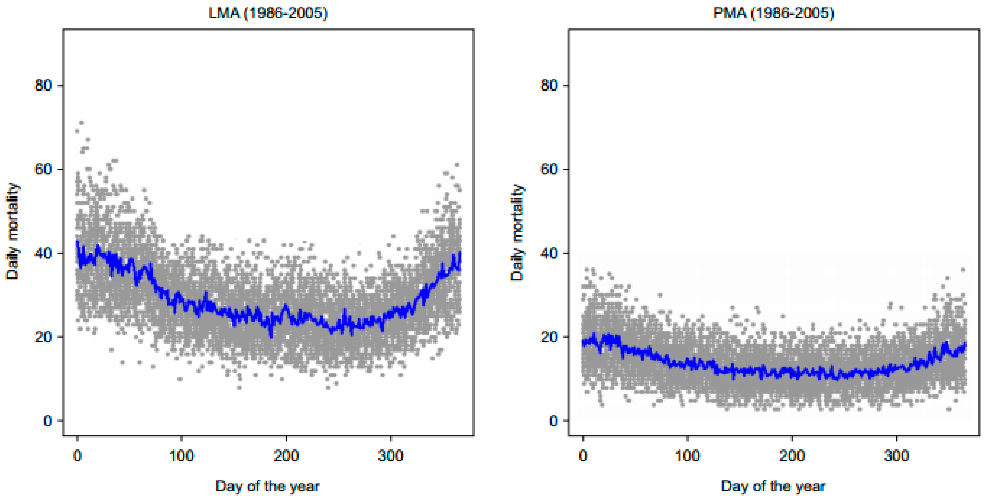
Figure 1. Seasonal distribution of daily mortality in Lisbon metropolitan area (LMA) and Porto metropolitan area (PMA). The grey dots are the actual number of deaths in each day of the year during the period from 1986 to 2005, and the blue line is the average daily mortality per day of the year projected into the future.
Atmosphere 10 00735 g001
Figure 2. Distribution of mean temperature in the historical period (1986–2005) and future periods (2046–2065 and 2080–2099). (A) Time series of temperature for the study period, (B) Changes in mean daily temperature for winter and summer seasons. The Representative Concentration Pathway (RCP8.5) greenhouse gas emission scenario is considered.
Atmosphere 10 00735 g002
Figure 3. Overall cumulative exposure–response curves for the relationship between daily temperatures and mortality for the historical data (1986–2005) over lags of 0–30 days for different model specifications. The minimum mortality temperature (dashed vertical line) stands as a reference. The broken thick black lines correspond to the 5th and 95th temperature percentiles.
Atmosphere 10 00735 g003
Figure 4. Lag-specific temperature–mortality relationships for lags of 0–30 days under different models and temperature exposures to 1st, 5th, and 10th temperature percentiles (cold effect) and 90th, 95th, and 99th temperature percentiles (hot temperature effect). The grey regions represent 95% confidence intervals.
Atmosphere 10 00735 g004
Figure 5. Temperature and excess mortality for the historical and future periods in the study region. Top panel: Exposure–response curve for temperature–mortality relative risk (RR), with the blue and red lines representing cold and hot, respectively, together with their 95% CI in grey. The solid vertical line corresponds to the mean temperature that divides the curve into cold and hot, while the dotted represents the reference temperature (MMT). The dashed red line represents the extrapolation beyond the maximum temperature in 1986–2005 (broken vertical line) for the future periods. Middle panel: Temperature distribution for the historical (grey area) and future periods, 2046–2065 (green area) and 2080–2099 (darker green area). Bottom panel: Temperature-related excess mortality distribution expressed as the fraction of additional deaths (%) attributed to non-optimal temperature, compared with the reference temperature.
Atmosphere 10 00735 g005
Figure 6. Temperature and excess mortality for the historical and future periods in the study region during the winter period. Top panel: Exposure–response curve for temperature–mortality relative risk (RR), with the blue and red lines representing cold and hot, respectively, together with their 95% CI in grey. The solid vertical line corresponds to the mean temperature that divides the curve into cold and hot, while the dotted represents the reference temperature (MMT). The dashed red line represents the extrapolation beyond the maximum temperature in 1986–2005 (broken vertical line) for the future periods. Middle panel: Temperature distribution for the historical (grey area) and future periods, 2046–2065 (green area) and 2080–2099 (darker green area). Bottom panel: Temperature-related excess mortality distribution expressed as the fraction of additional deaths (%) attributed to non-optimal temperature, compared with the reference temperature.
Atmosphere 10 00735 g006
Figure 7. Temperature and excess mortality for the historical and future periods in the study region during the summer period. Top panel: Exposure–response curve for temperature–mortality relative risk (RR), with the blue and red lines representing cold and hot, respectively, together with their 95% CI in grey. The solid vertical line corresponds to the mean temperature that divides the curve into cold and hot, while the dotted represents the reference temperature (MMT). The dashed red line represents the extrapolation beyond the maximum temperature in 1986–2005 (broken vertical line) for the future periods. Middle panel: Temperature distribution for the historical (grey area) and future periods, 2046–2065 (green area) and 2080–2099 (darker green area). Bottom panel: Temperature-related excess mortality distribution expressed as the fraction of additional deaths (%) attributed to non-optimal temperature, compared with the reference temperature.
Atmosphere 10 00735 g007
Figure 8. Total attributable risk of mortality due to combined hot/cold for different degrees of freedom and temperature variables. Temp: Using minimum temperature in winter and maximum temperature in summer (original variable used) vs. Tmin: Using minimum temperatures.
Atmosphere 10 00735 g008
Table 1. Region-specific summary statistics of mortality from circulatory system diseases (CSD) and daily temperatures (°C), for the whole year, summer and winter months, for Portuguese metropolitan areas (Mean, IQR a).
Metropolitan AreaSeasonTotal DeathsDaily Temperature (1986–2005)Projected Temperature (2046–2065)Projected Temperature (2080–2099)d MMT (95% CI)
LisbonFull year209,96415.4 (11.4–21.3) a17.0 (12.6–23.7)18.5 (13.7–25.8)26 (24.8–27.1)
Summer58,37623.3 (21.1–26.4) c25.8 (23.4–28.8)28.1 (25.7–31.1
Winter86,5599.8 (7.6–11.9) b10.9 (9.2–13.0)12.0 (10.4–14.2)
PortoFull year100,28014.5 (10.0–26.0) a15.9 (11.0–23.7)17.5 (12.2–26.3)29.9 (24.1–41.5)
Summer28,02923.1 (21.2–26.0) c25.5 (23.6–28.8)28.2 (26.2–31.2)
Winter40,7227.8 (4.7–10.4) b8.9 (6.4–11.3)10.0 (7.7–12.4)
a IQR: Interquartile range; Temperature: b Minimum Temperature for winter; c Maximum temperature for summer; d MMT: minimum mortality temperature; CI: confidence interval.
Table 2. Estimated risk (95% confidence interval), attributable mortality with 95% empirical CI, excess mortality attributable to temperature in the future periods (2046–2065 and 2080–2099) in relation to the historical period (1986–2005) evaluated at extreme temperatures.
Metropolitan Area/SeasonTemperatureRR (95% CI)AN (95% eCI)AF% (95% eCI)AF rel (%)
Historical (1986–2005)
Lisbon/Full year1th percentile: 4.52.30 (1.84, 2.88)1546.67 (1294.51, 1730.92)0.74 (0.62, 0.82)0
99th percentile: 33.71.03 (0.96, 1.09)92.70 (−34.73, 183.78)0.04 (−0.02, 0.09)0
Lisbon/Winter1th percentile: 3.01.45 (1.16, 1.82)1894.54 (1378.90, 2312.19)0.67 (0.49, 0.82)0
99th percentile: 16.31.67 (1.41, 1.99)316.47 (145.23, 451.03)0.11 (0.05, 0.16)0
Lisbon/Summer1th percentile: 17.71.01 (0.97, 1.05)37.98 (−227.48, 294.64)0.02 (−0.14, 0.18)0
99th percentile: 36.31.09 (1.00, 1.19)59.39 (−2.66, 116.64)0.04 (0.00, 0.07)0
Porto/Full year1th percentile: 0.702.07 (1.66, 2.58)811.95 (691.33, 910.25)0.81 (0.69, 0.91)0
99th percentile: 33.301.00 (0.95, 1.06)8.64 (−47.03, 54.79)0.01 (−0.05, 0.05)0
Porto/Winter1th percentile: −0.51.82 (1.41, 2.34)382.95 (−108.21, 802.38)0.14 (−0.04, 0.28)0
99th percentile: 14.42.43 (1.91, 3.10)2868.99 (2093.18, 3374.93)1.02 (0.74, 1.20)0
Porto/Summer1th percentile: 181.01 (0.97, 1.05)5.86 (−25.46, 34.17)0 (−0.02, 0.02)0
99th percentile: 35.21.00 (0.98, 1.02)14.28 (−69.73, 89.78)0.01 (−0.04, 0.05)0
Future (2046–2065)
Lisbon/Full year1th percentile: 6.91.81 (1.45, 2.25)231.83 (193.49, 259.78)0.11 (0.09, 0.12)−0.63 (−0.7, −0.52)
99th percentile: 36.41.03 (0.95, 1.12)298.43 (−118.67, 592.22)0.14 (−0.06, 0.28)0.10 (−0.04, 0.19)
Lisbon/Winter1th percentile: 5.51.39 (1.25, 1.55)259.29 (189.10, 316.34)0.09 (0.07, 0.11)−0.58 (−0.71, −0.42)
99th percentile: 17.11.47 (1.10, 1.98)887.76 (264.19, 1308.12)0.31 (0.09, 0.46)0.20 (0.04, 0.30)
Lisbon/Summer1th percentile: 19.11.00 (0.98, 1.03)9.50 (−60.04, 79.43)0.01 (−0.04, 0.05)−0.02 (−0.13, 0.10)
99th percentile: 38.41.11 (1.00, 1.25)188.91 (−9.35, 371.79)0.11 (−0.01, 0.22)0.08 (0.00, 0.15)
Porto/Full year1th percentile: 2.51.64 (1.33, 2.03)192.51 (168.52, 209.75)0.19 (0.17, 0.21)−0.62 (−0.70, −0.52)
99th percentile: 36.41.03 (0.85, 1.24)54.82 (−259.08, 292.64)0.05 (−0.26, 0.29)0.05 (−0.22, 0.24)
Porto/Winter1th percentile: 1.31.37 (1.17, 1.61)49.95 (−13.44, 105.34)0.02 (0.00, 0.04)−0.12 (−0.25, 0.03)
99th percentile: 15.42.92 (2.03, 4.19)6459.91 (4563.58, 7642.42)2.29 (1.62, 2.71)1.27 (0.88, 1.52)
Porto/Summer1th percentile: 19.11.01 (0.97, 1.05)0.45 (−2.02, 2.68)0 (0.00, 0.00)0 (−0.02, 0.01)
99th percentile: 37.51.00 (0.97, 1.04)21.85 (−122.99, 157.10)0.01 (−0.07, 0.09)0.00 (−0.04, 0.04)
Future (2080–2099)
Lisbon/Full year1th percentile: 8.61.69 (1.36, 2.10)25.03 (20.45, 28.34)0.01 (0.01, 0.01)−0.73 (−0.81, −0.61)
99th percentile: 39.41.37 (0.89, 2.10)1050.35 (−462.24, 1898.65)0.50 (−0.22, 0.90)0.46 (−0.21, 0.82)
Lisbon/Winter1th percentile: 7.11.38 (1.23, 1.55)23.42 (16.53, 29.06)0.01 (0.01, 0.01)−0.66 (−0.81, −0.48)
99th percentile: 18.51.20 (0.65, 2.22)1820.53 (−387.48, 3054.90)0.65 (−0.14, 1.08)0.53 (−0.18, 0.92)
Lisbon/Summer1th percentile: 20.61.00 (0.99, 1.01)1.10 (−8.91, 10.95)0.00 (−0.01, 0.01)−0.02 (−0.17, 0.13)
99th percentile: 42.21.14 (0.97, 1.36)444.65 (−30.75, 891.90)0.27 (−0.02, 0.54)0.23 (−0.02, 0.47)
Porto/Full year1th percentile: 3.91.56 (1.27, 1.93)120.83 (105.94, 131.60)0.12 (0.11, 0.13)−0.69 (−0.78, −0.58)
99th percentile: 39.31.14 (0.65, 1.99)216.01 (−1004.00, 890.65)0.22 (−1.00, 0.89)0.21 (−0.98, 0.83)
Porto/Winter1th percentile: 2.81.11 (1.00, 1.24)5.14 (−5.64, 14.37)0.00 (0.00, 0.01)−0.13 (−0.28, 0.04)
99th percentile: 17.12.49 (1.36, 4.56)10761.18 (6706.74, 13068.30)3.81 (2.38, 4.63)2.80 (1.63, 3.44)
Porto/Summer1th percentile: 20.61.01 (0.97, 1.05)0.24 (−2.53, 3.29)0 (0.00, 0.00)0 (−0.02, 0.02)
99th percentile: 41.21.00 (0.95, 1.06)24.58 (−158.76, 187.31)0.01(−0.10, 0.11)0.01 (−0.06, 0.06)
* Notes: Bold face represents significant effects.