Observing and Modeling the Response of Placentia Bay to an Extratropical Cyclone


Abstract
1. Introduction
2. Data and Model Description
2.1. Data
2.1.1. Remote Sensing Data
2.1.2. In Situ Data
2.1.3. Numerical Model Data
2.2. Model
2.2.1. FVCOM (3.2) Ocean Circulation Model
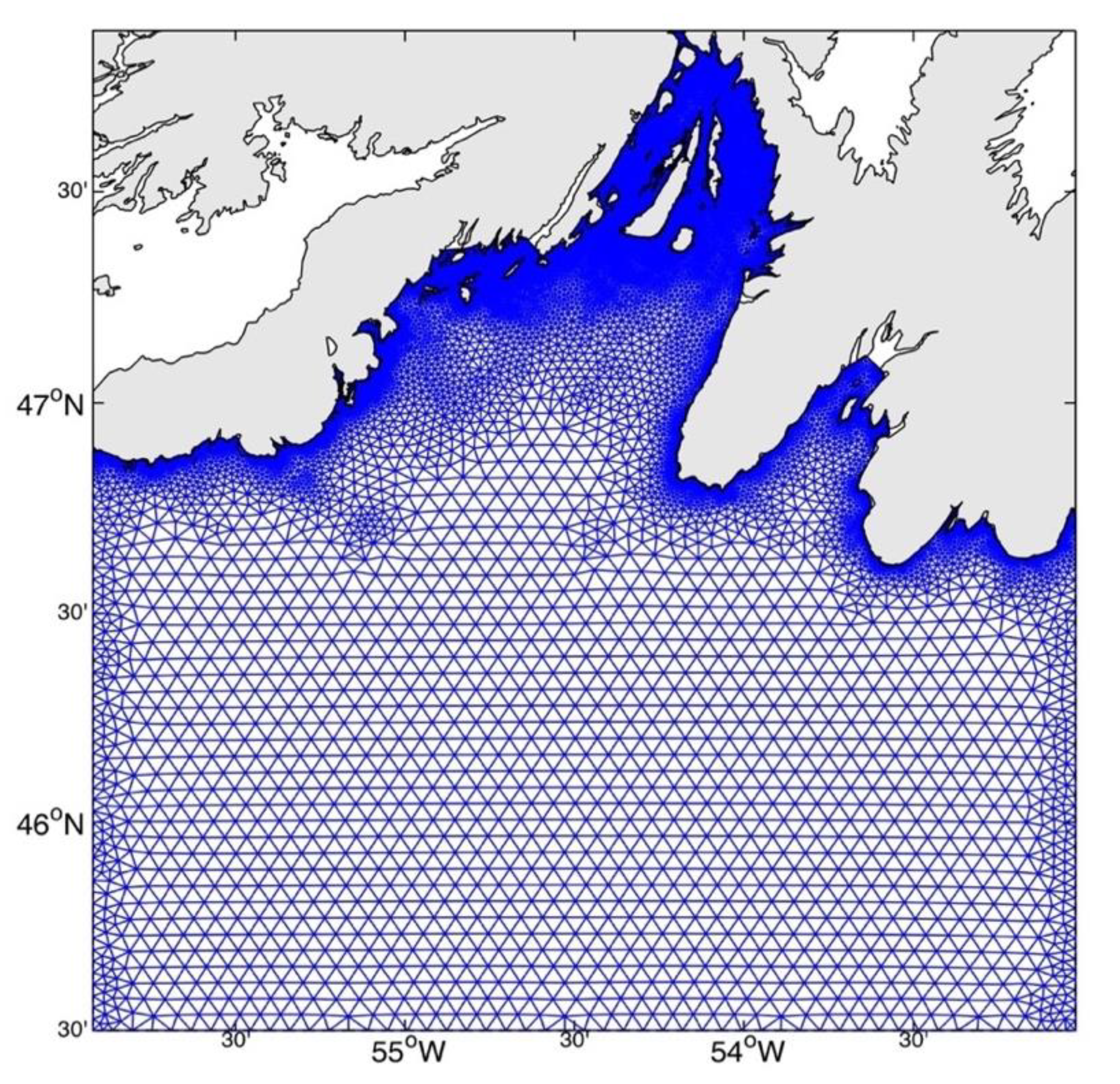
2.2.2. Model Domain and Grid
2.2.3. Model Forcing, Open Boundary Conditions and Initial Conditions
2.2.4. Model Validation Metrics
3. Results
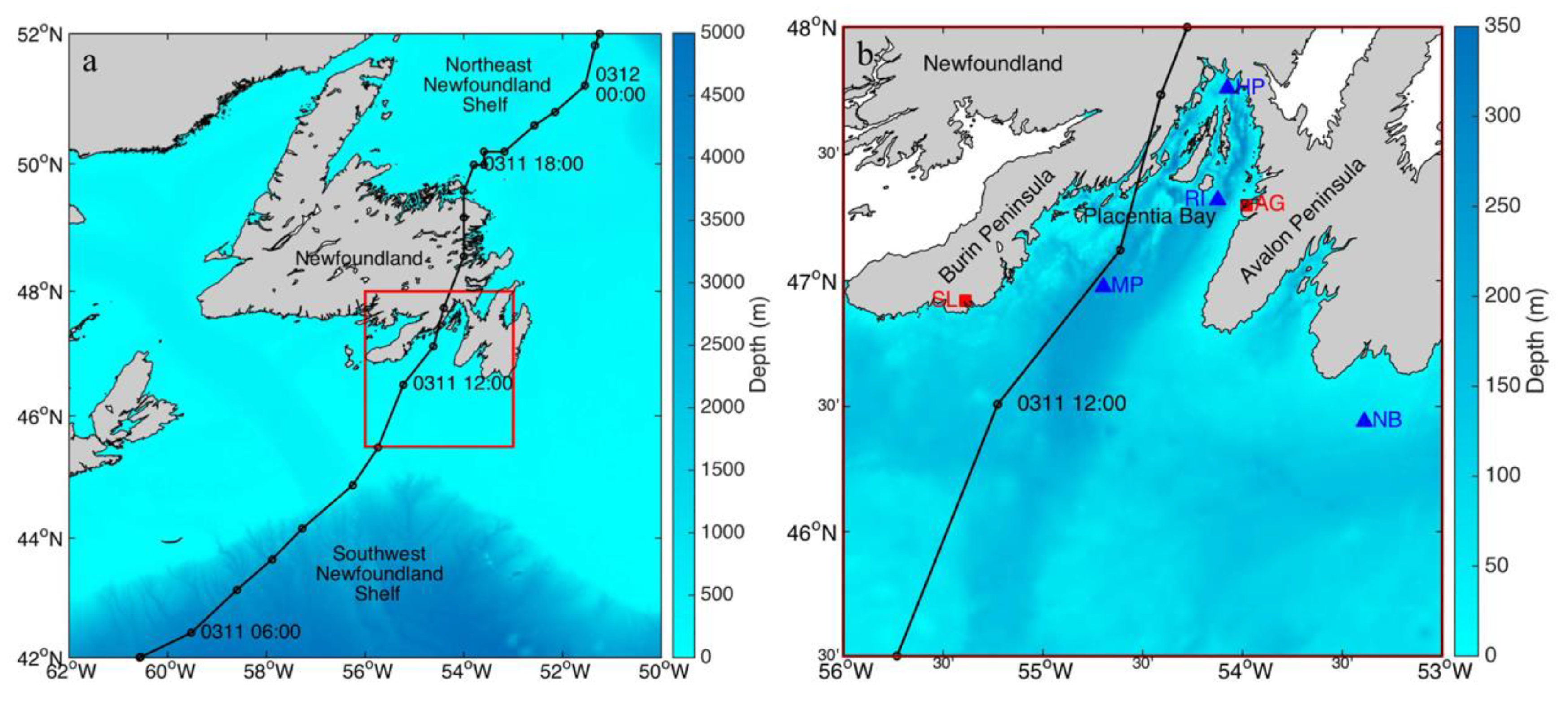
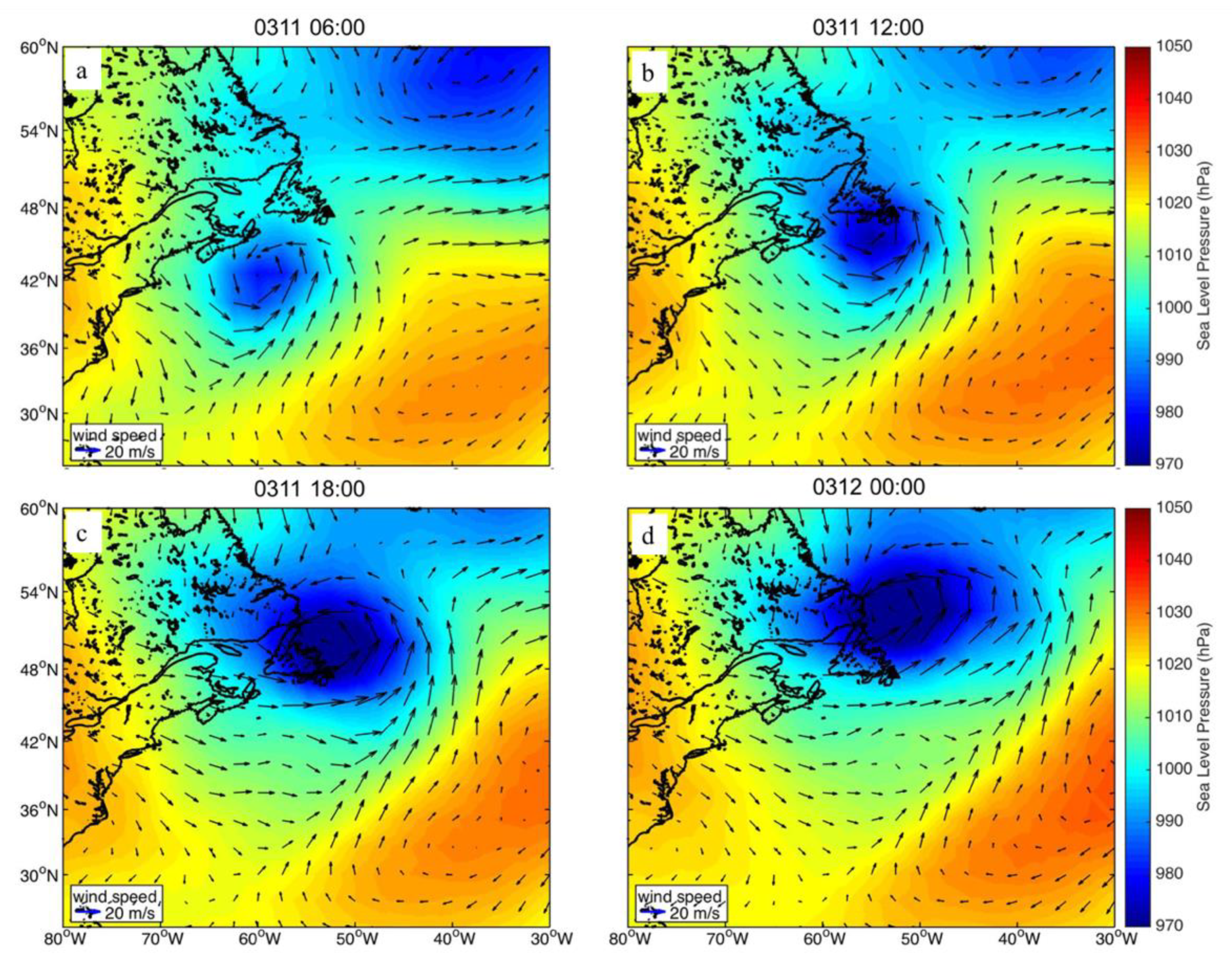
3.1. Extratropical Storm Detection
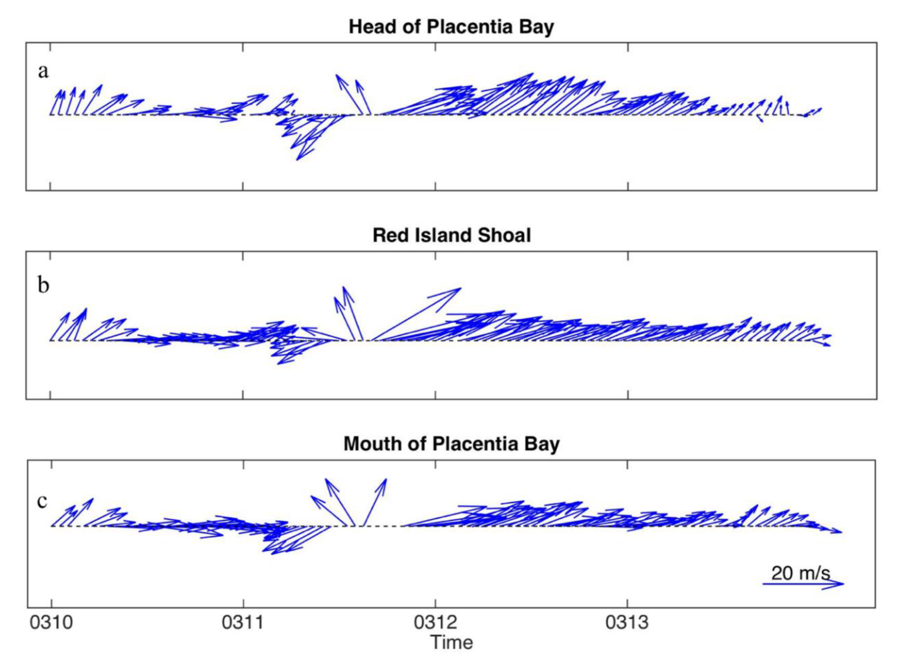
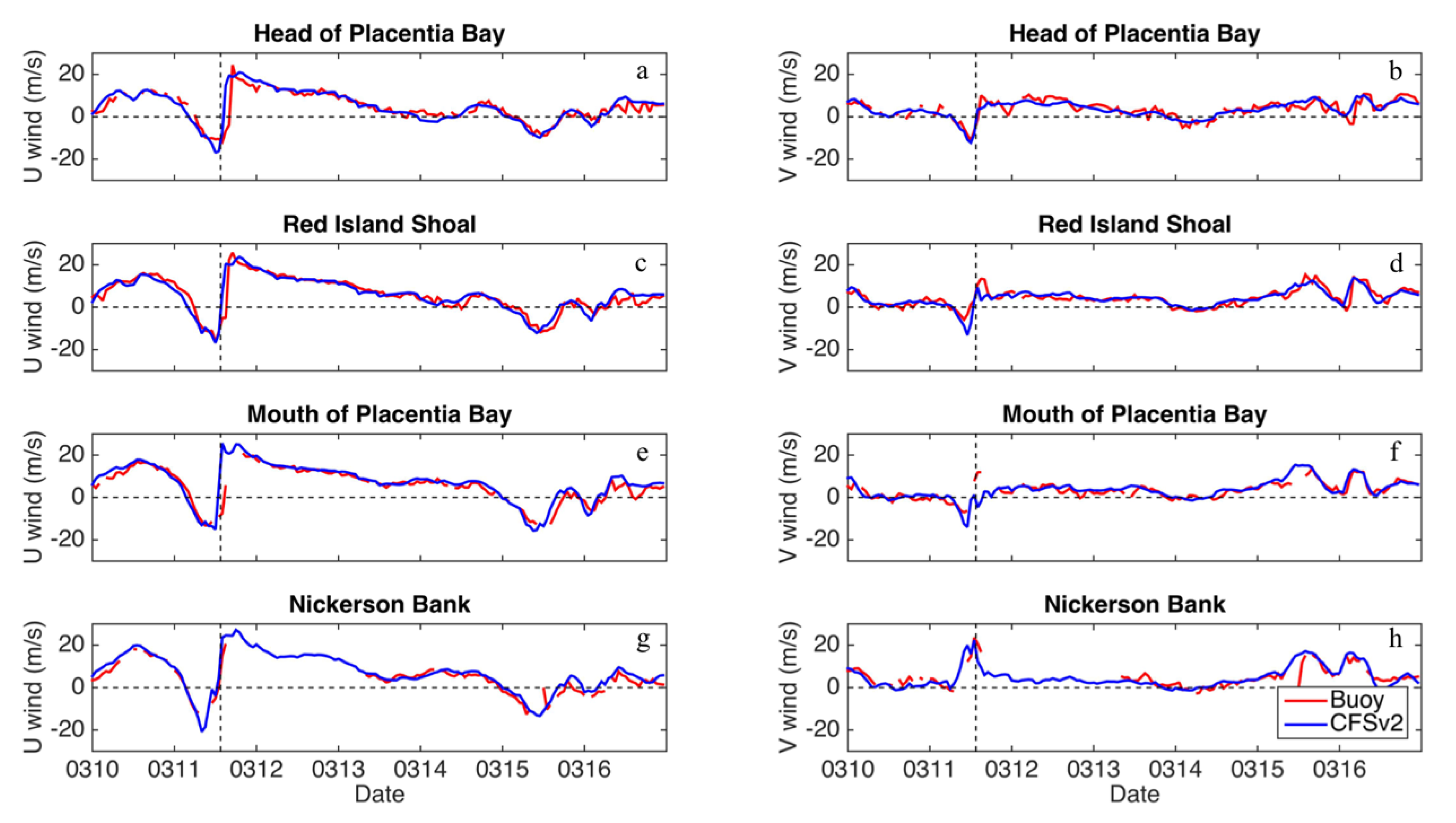
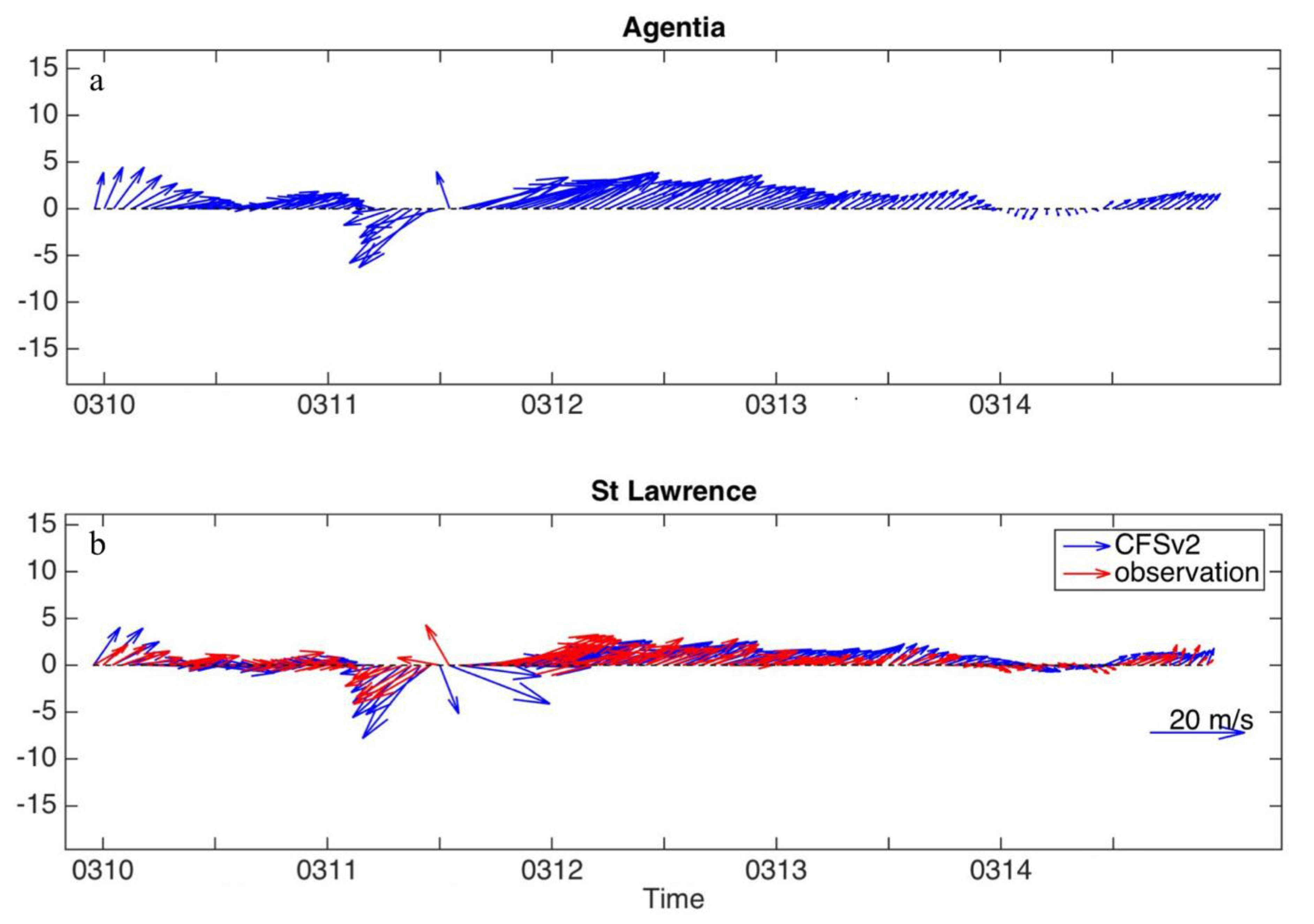
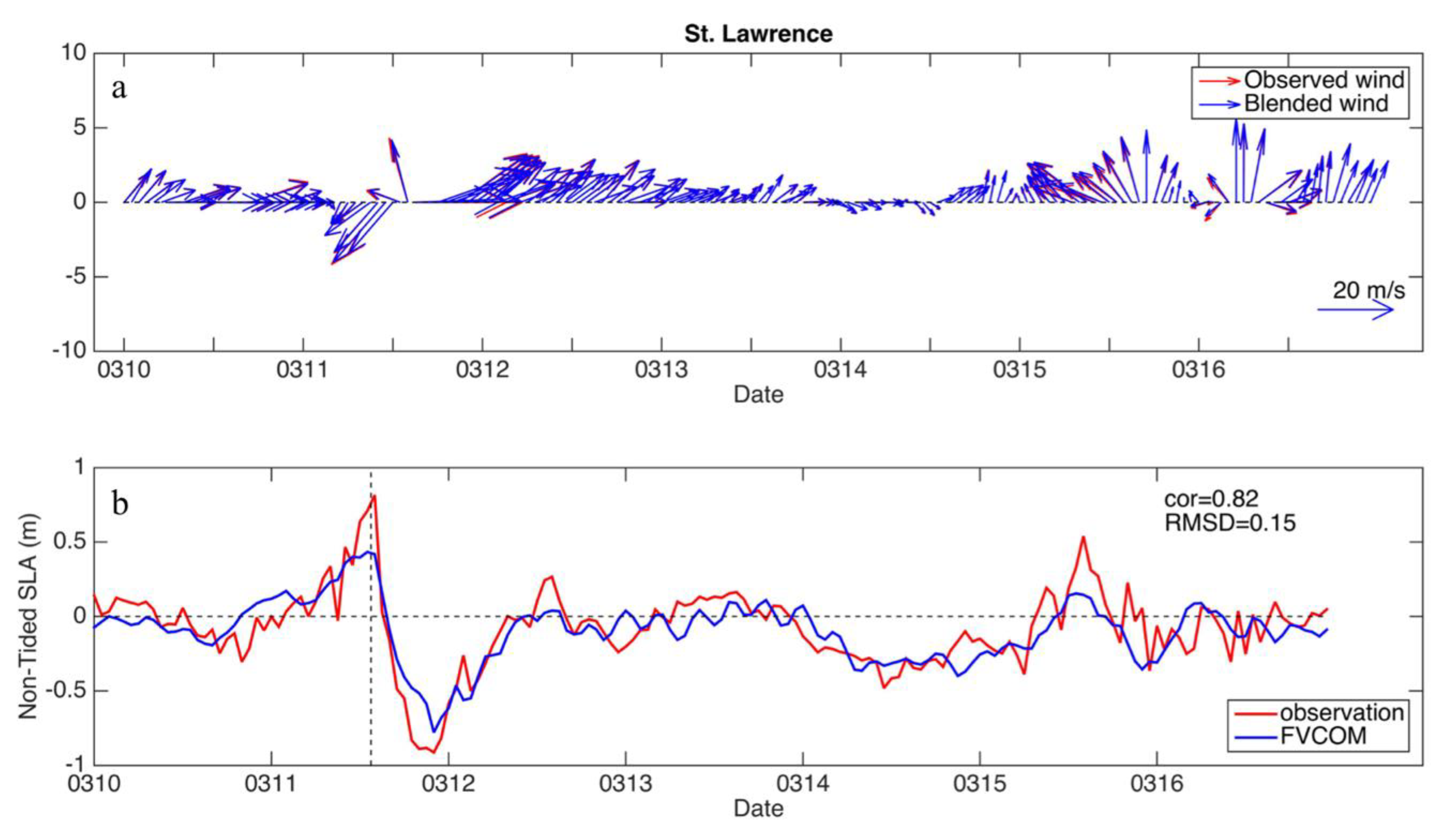
3.2. Wind
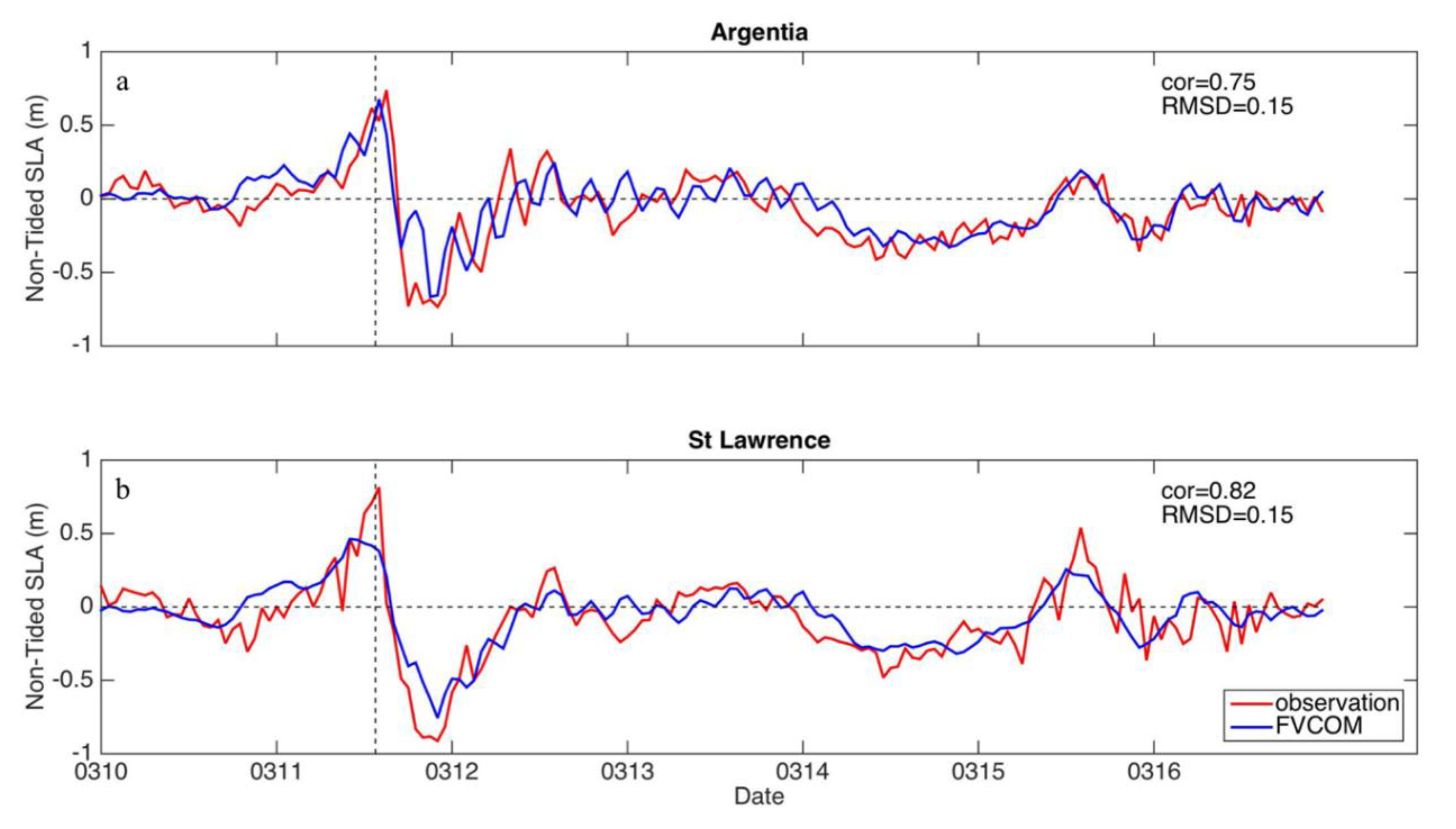
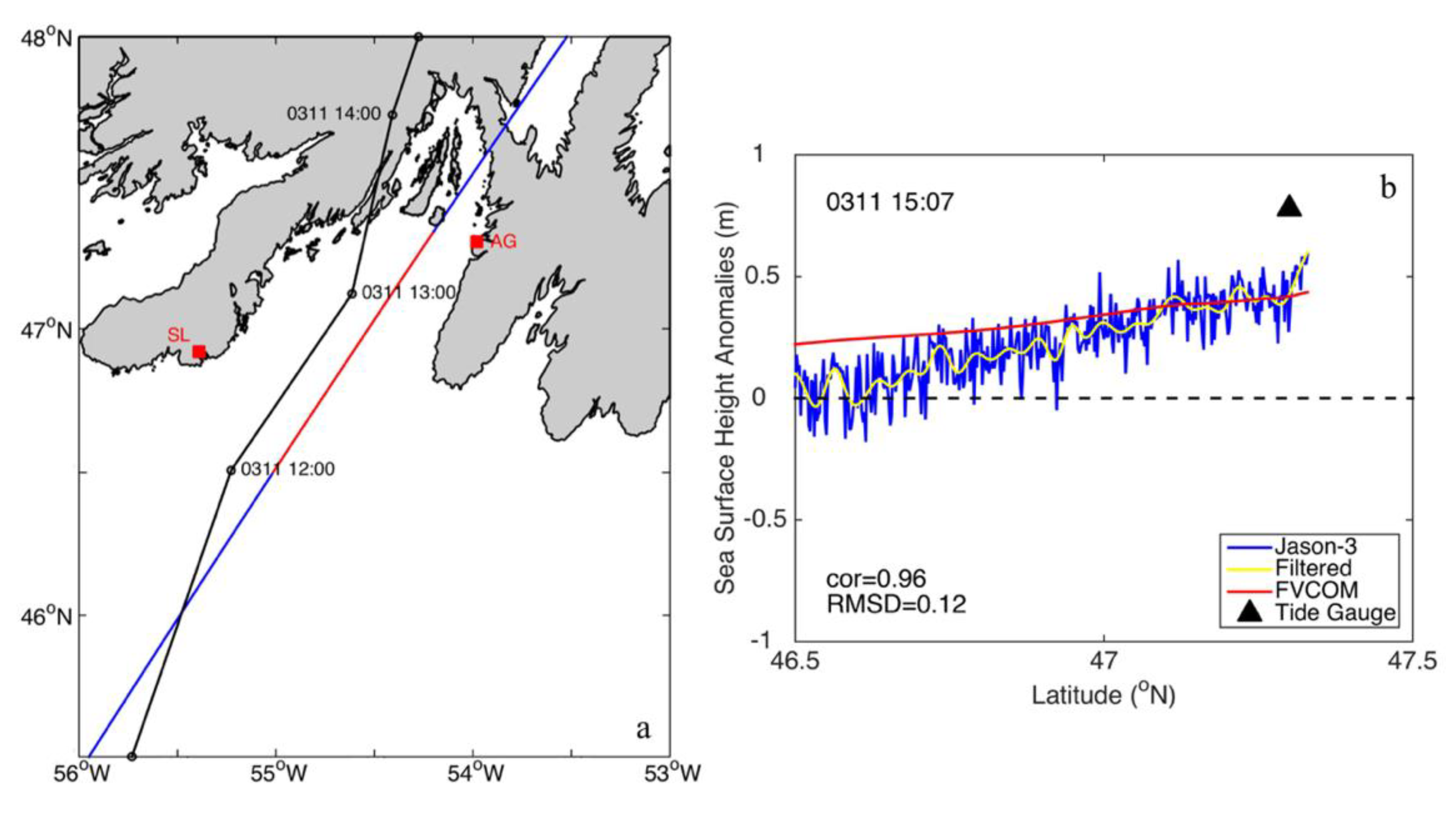
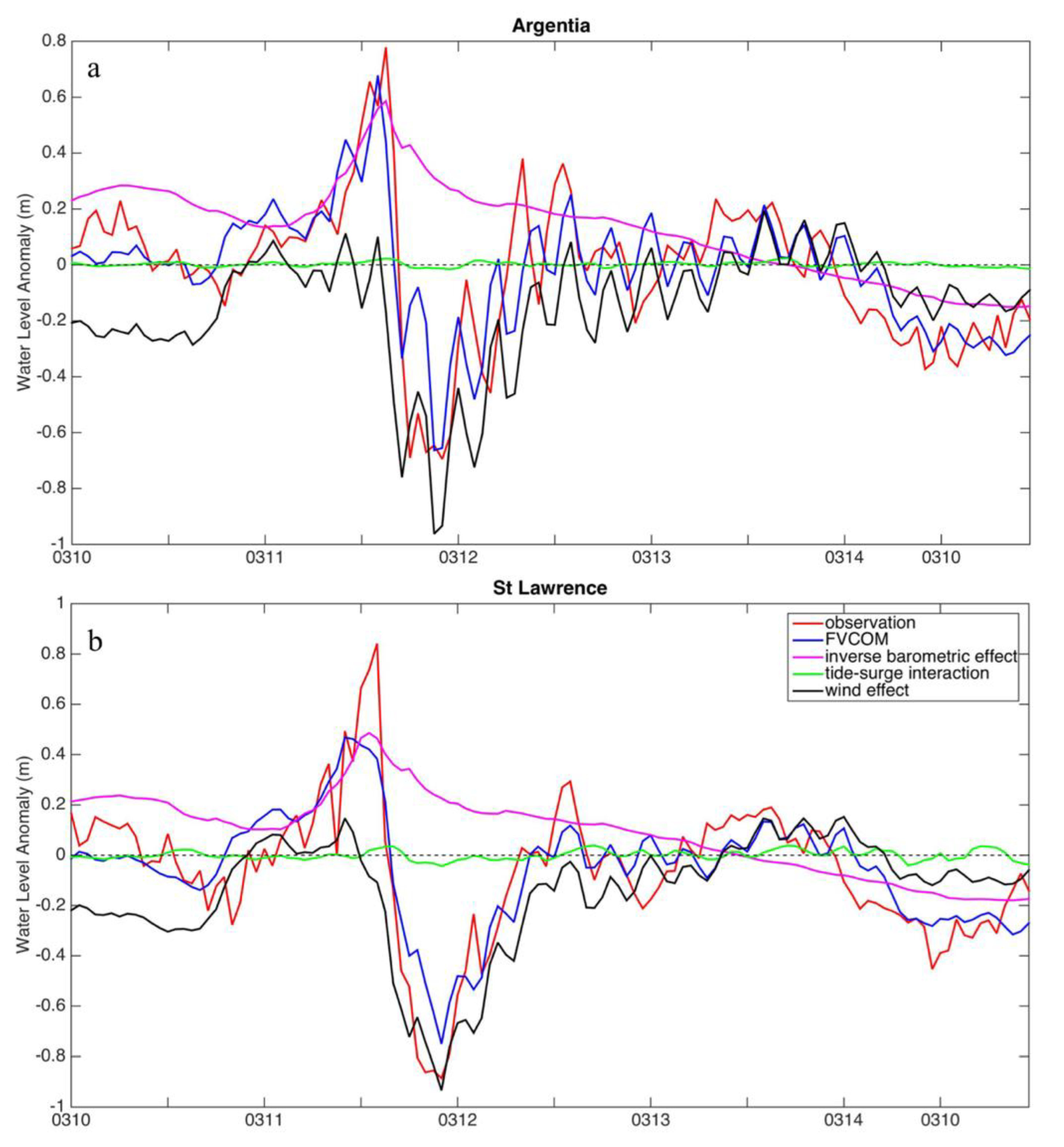
3.3. Storm Surge
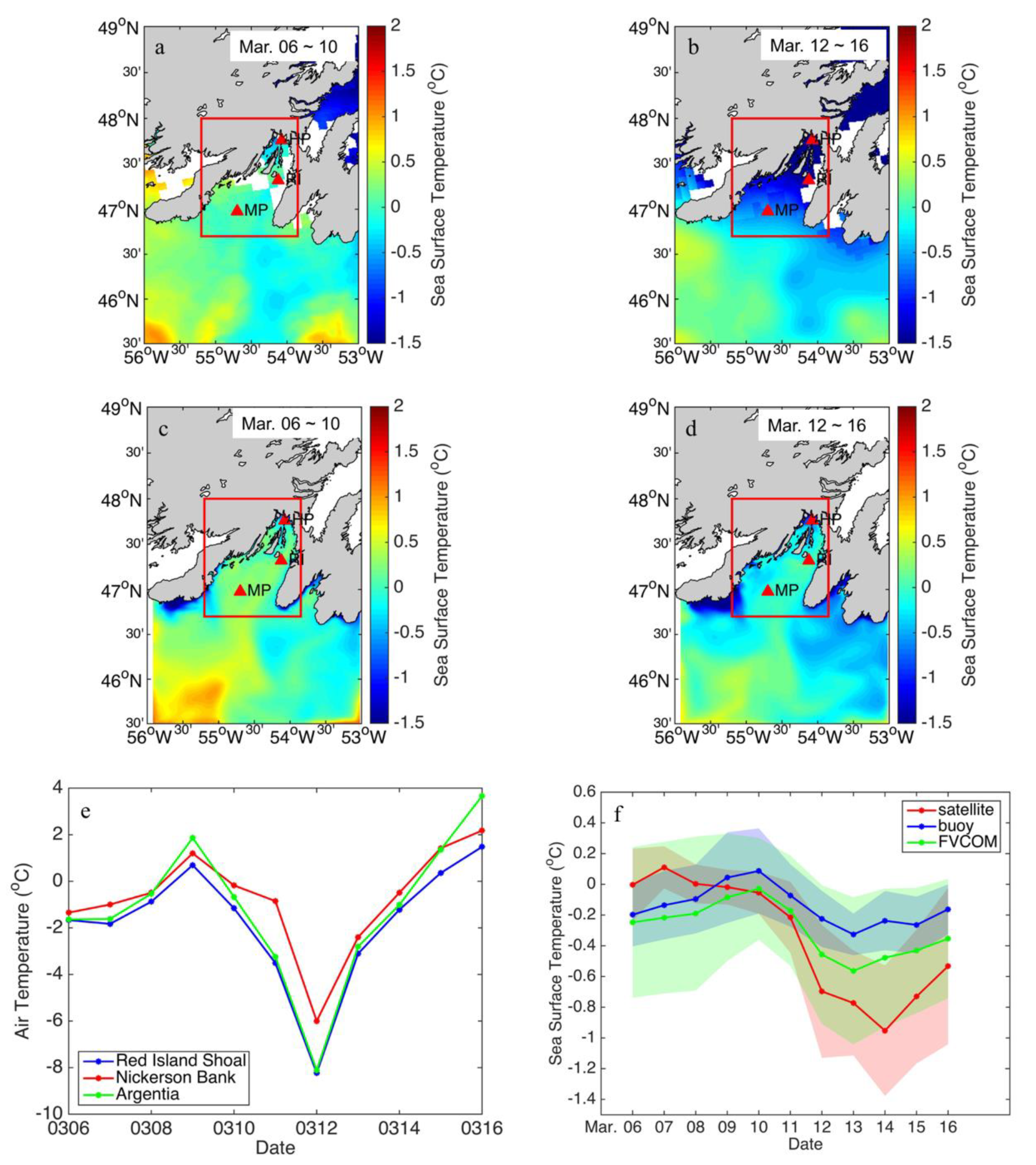
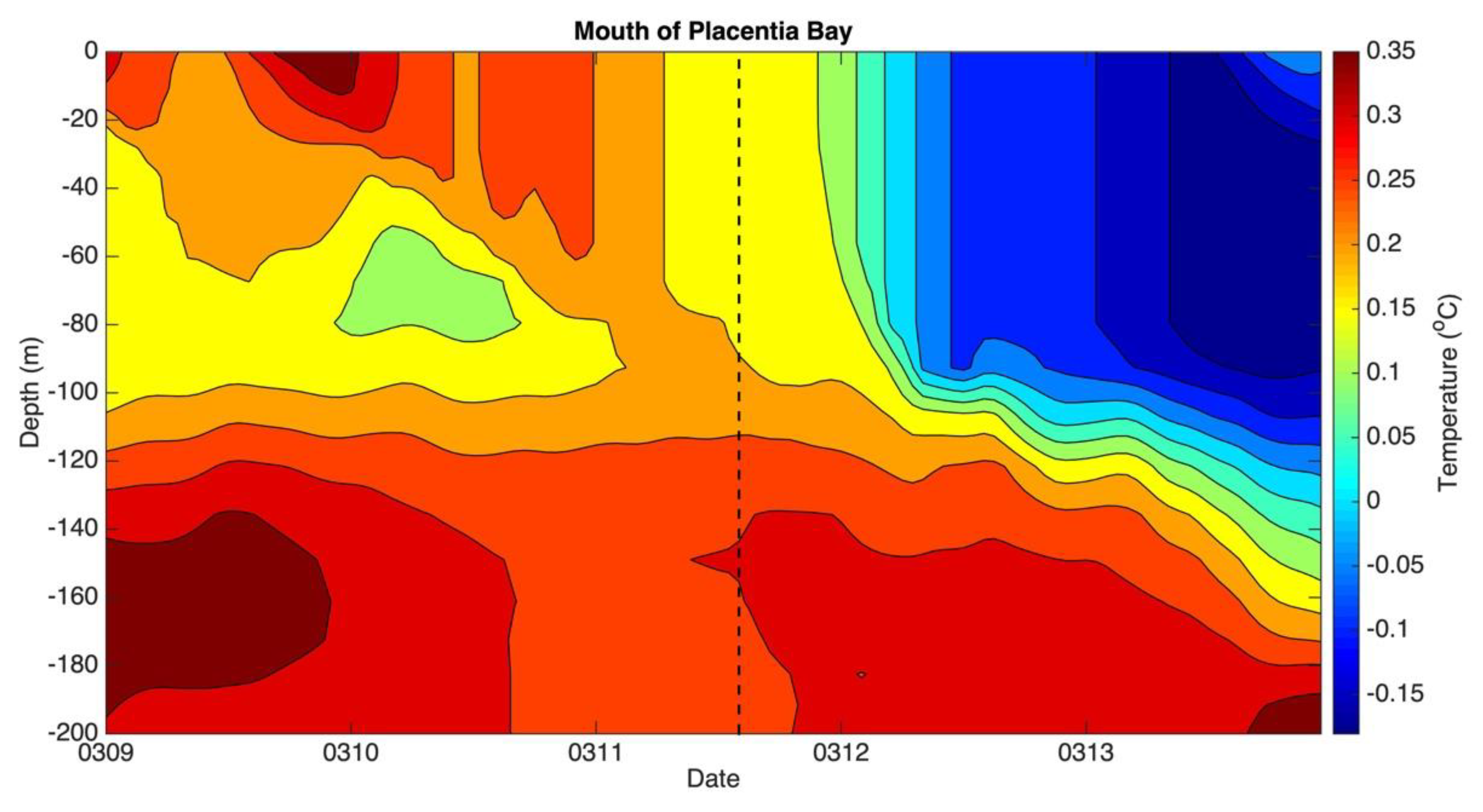
3.4. Temperature
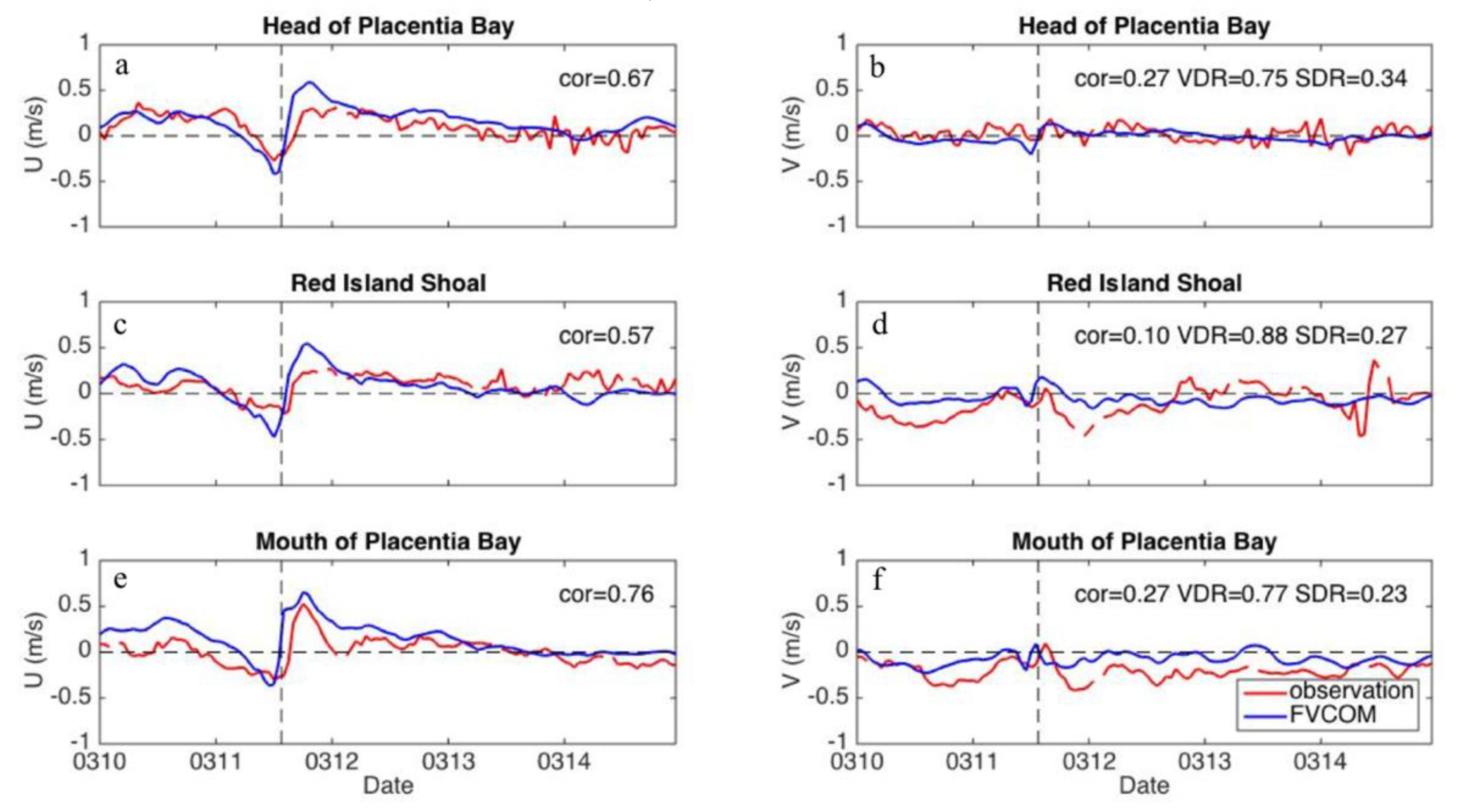
3.5. Sea Surface Current
4. Discussion
4.1. Storm Surge Mechanisms
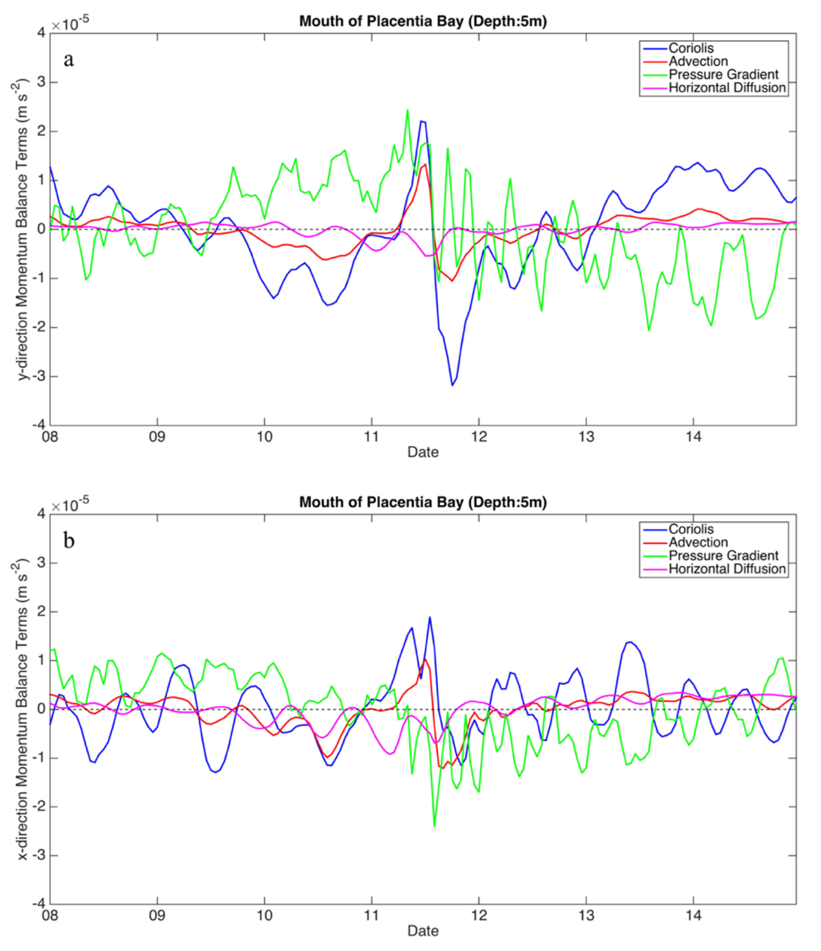
4.2. Momentum Balance
4.3. Differences in Responses to Winter and Summer Storms
5. Summary and Conclusions
Author Contributions
Funding
Acknowledgments
Conflicts of Interest
References
- Bernier, N.B.; Thompson, K.R. Predicting the frequency of storm surges and extreme sea levels in the Northwest Atlantic. J. Geophys. Res. Ocean. 2006, 111, C10009. [Google Scholar] [CrossRef]
- Chen, C.; Beardsley, R.C.; Luettich, A.L., Jr.; Westerink, J.J.; Wang, H.; Perrie, W.; Xu, Q.; Donahue, A.S.; Qi, J.; Lin, H.; et al. Extratropical storm inundation tested: Inter-model comparisons in Scituate, Massachusetts. J. Geophys. Res. Ocean. 2013, 118, 5054–5073. [Google Scholar] [CrossRef]
- Bradbury, I.R.; Snelgrove, P.V.; Fraser, S. Transport and development of eggs and larvae of Atlantic cod, Gadus morhua, in relation to spawning time and location in coastal Newfoundland. Can. J. Fish. Aquat. Sci. 2000, 57, 1761–1772. [Google Scholar] [CrossRef]
- Han, G.; Ma, Z.; Chen, D.; DeYoung, B.; Chen, N. Observing storm surges from space: Hurricane Igor off Newfoundland. Sci. Rep. 2012, 2, 1010. [Google Scholar] [CrossRef] [PubMed]
- Ma, Z.; Han, G.; DeYoung, B. Oceanic responses to Hurricane Igor over the Grand Banks: A modeling study. J. Geophys. Res. Ocean. 2015, 120, 1276–1295. [Google Scholar] [CrossRef]
- Han, G.; Ma, Z.; Chen, N. Hurricane Igor impacts on the stratification and phytoplankton bloom over the Grand Banks. J. Mar. Syst. 2012, 100, 19–25. [Google Scholar] [CrossRef]
- Ma, Z.; Han, G.; DeYoung, B. Modelling the response of Placentia Bay to hurricanes Igor and Leslie. Ocean Model. 2017, 112, 112–124. [Google Scholar] [CrossRef]
- Catto, J.L. Extratropical cyclone classification and its use in climate studies. Rev. Geophys. 2016, 54, 486–520. [Google Scholar] [CrossRef]
- Orton, P.M.; Hall, T.M.; Talke, S.A.; Blumberg, A.F.; Georgas, N.; Vinogradov, S. A validated tropical-extratropical flood hazard assessment for New York Harbor. J. Geophys. Res. Ocean. 2016, 121, 8904–8929. [Google Scholar] [CrossRef]
- Hirsch, M.E.; DeGaetano, A.T.; Colucci, S.J. An East Coast Winter Storm Climatology. J. Clim. 2001, 14, 882–899. [Google Scholar] [CrossRef]
- Colle, B.A.; Booth, J.F.; Chang, E.K.M. A review of historical and future changes of extratropical cyclones and associated impacts along the US East Coast. Curr. Clim. Chang. Rep. 2015, 1, 125–143. [Google Scholar] [CrossRef]
- DeGaetano, A.T. Predictability of seasonal east coast winter storm surge impacts with application to New York’s Long Island. Meteorol. Appl. 2008, 15, 231–242. [Google Scholar] [CrossRef]
- Booth, J.F.; Rieder, H.E.; Lee, D.E.; Kushnir, Y. The paths of extratropical cyclones associated with wintertime high-wind events in the northeastern United States. J. Appl. Meteorol. Clim. 2015, 54, 1871–1885. [Google Scholar] [CrossRef]
- Nelson, J.; He, R. Effect of the Gulf Stream on winter extratropical cyclone outbreaks. Atmos. Sci. Lett. 2012, 13, 311–316. [Google Scholar] [CrossRef]
- Hurricane-force Winds Wreak Havoc in Newfoundland. Available online: https://www.theglobeandmail.com/news/national/brier-play-stopped-as-extreme-winds-batter-newfoundland/article34275289/ (accessed on 17 April 2017).
- Valladeau, G.; Thibaut, P.; Picard, B.; Poisson, J.C.; Tran, N.; Picot, N.; Guillot, A. Using SARAL/AltiKa to improve Ka-band altimeter measurements for coastal zones, hydrology and ice: The PEACHI prototype. Mar. Geod. 2015, 38 (Suppl. 1), 124–142. [Google Scholar] [CrossRef]
- Ray, R.D. Precise comparisons of bottom-pressure and altimetric ocean tides. J. Geophys. Res. Ocean. 2013, 118, 4570–4584. [Google Scholar] [CrossRef]
- Cartwright, D.E.; Edden, A.C. Corrected tables of tidal harmonics. Geophys. J. R. Astron. Soc. 1973, 33, 253–264. [Google Scholar] [CrossRef]
- Wahr, J.M. Deformation induced by polar motion. J. Geophys. Res. Solid Earth 1985, 90, 9363–9368. [Google Scholar] [CrossRef]
- Martin, M.; Dash, P.; Ignatov, A.; Banzon, V.; Beggs, H.; Brasnett, B.; Cayula, J.F.; Cummings, J.; Donlon, C.; Gentemann, C.; et al. Group for High Resolution Sea Surface Temperature (GHRSST) analysis fields inter-comparisons. Part 1: A GHRSST multi-product ensemble (GMPE). Deep Sea Res. Part II 2012, 77–80, 21–30. [Google Scholar] [CrossRef]
- Dash, P.; Ignatov, A.; Martin, M.; Donlon, C.; Brasnett, B.; Reynolds, R.W.; Banzon, V.; Beggs, H.; Cayula, J.F.; Chao, Y.; et al. Group for High Resolution Sea Surface Temperature (GHRSST) analysis fields inter-comparisons—Part 2: Near real time web-based level 4 SST Quality Monitor (L4-SQUAM). Deep Sea Res. Part II 2012, 77–80, 31–43. [Google Scholar] [CrossRef]
- Saha, S.; Moorthi, S.; Wu, X.; Wang, J.; Nadiga, S.; Tripp, P.; Behringer, D.; Hou, Y.T. The NCEP climate forecast system version 2. J. Clim. 2014, 27, 2185–2208. [Google Scholar] [CrossRef]
- Bleck, R.; Halliwell, G.R., Jr.; Wallcraft, A.J.; Carroll, S.; Kelly, K.; Rushing, K. Hybrid Coordinate Ocean Model (HYCOM) User’s Manual: Details of the Numerical Code. Available online: http://hycom.rsmas.miami.edu (accessed on 12 May 2017).
- Chen, C.; Liu, H.; Beardsley, R.C. An unstructured grid, finite-volume, three-dimensional, primitive equations ocean model: Application to coastal ocean and estuaries. J. Atmos. Ocean. Technol. 2003, 20, 159–186. [Google Scholar] [CrossRef]
- Rego, J.L.; Li, C. Storm surge propagation in Galveston Bay during Hurricane Ike. J. Mar. Syst. 2010, 82, 265–279. [Google Scholar] [CrossRef]
- Han, G.; Ma, Z.; DeYoung, B.; Foreman, M.; Chen, N. Simulation of three-dimensional circulation and hydrography over the Grand Banks of Newfoundland. Ocean Model. 2011, 40, 199–210. [Google Scholar] [CrossRef]
- Burchard, H.; Bolding, K.; Villarreal, M.R. GOTM, a General Ocean Turbulence Model: Theory, Implementation and Test Cases; Technical Reports; Space Applications Institute: Gujarat, India, 1999. [Google Scholar]
- Mellor, G.L.; Ezer, T.; Oey, L.Y. The pressure gradient conundrum of sigma coordinates ocean models. J. Atmos. Ocean. Technol. 1994, 11, 1126–1134. [Google Scholar] [CrossRef]
- Ma, Z.; Han, G.; DeYoung, B. Modelling temperature, currents and stratification in Placentia Bay. Atmos. Ocean 2012, 50, 244–260. [Google Scholar] [CrossRef]
- Egbert, G.D.; Erofeeva, S.Y. Efficient inverse modeling of barotropic ocean tides. J. Atmos. Ocean. Technol. 2002, 19, 183–204. [Google Scholar] [CrossRef]
- Dong, C.; McWilliams, J.C.; Hall, A.; Hughes, M. Numerical simulation of a synoptic event in the Southern California Bight. J. Geophys. Res. Ocean. 2011, 116, C05018. [Google Scholar] [CrossRef]
- Jiang, J.; Perrie, W. The impacts of climate change on autumn north Atlantic midlatitude cyclones. J. Clim. 2007, 20, 1174–1187. [Google Scholar] [CrossRef]
- Yao, Y.; Perrie, W.; Zhang, W.; Jiang, J. Characteristics of atmosphere-ocean interactions along North Atlantic extratropical storms tracks. J. Geophys. Res. Atmos. 2008, 113, D14124. [Google Scholar] [CrossRef]
- Han, G.; Lu, Z.; Wang, Z.; Helbig, J.; Chen, N.; DeYoung, B. Seasonal variability of the Labrador Current and shelf circulation off Newfoundland. J. Geophys. Res. Ocean. 2008, 113, C10013. [Google Scholar] [CrossRef]
- Pawlowicz, R.; Beardsley, B.; Lentz, S. Classical tidal harmonic analysis including error estimates in MATLAB using T_TIDE. Comput. Geosci. 2002, 28, 929–937. [Google Scholar] [CrossRef]
- Han, G.; Ma, Z.; Chen, N.; Chen, N.; Yang, J.; Chen, D. Hurricane Isaac storm surges off Florida observed by Jason-1 and Jason-2 satellite altimeters. Remote Sens. Environ. 2017, 198, 244–253. [Google Scholar] [CrossRef]
- Sheng, J.; Zhai, X.; Greatbatch, R.J. Numerical study of the storm-induced circulation on the Scotian Shelf during Hurricane Juan using a nested-grid ocean model. Prog. Oceanogr. 2006, 70, 233–254. [Google Scholar] [CrossRef]
- Bunya, S.; Dietrich, J.C.; Westerink, J.J.; Ebersole, B.B.; Smith, J.M.; Atkinson, J.H.; Jensen, R.; Resio, D.T.; Luettich, R.A.; Dawson, C.; et al. A high-resolution coupled riverine flow, tide, wind, wind wave, and storm surge model for Southern Louisiana and Mississippi. Part I: Model Development and Validation. Mon. Weather Rev. 2010, 138, 345–377. [Google Scholar] [CrossRef]
- Mecking, J.V.; Fogarty, C.T.; Greatbatch, R.J.; Sheng, J.; Mercer, D. Using atmospheric model output to simulate the meteorological tsunami response to Tropical Storm Helene (2000). J. Geophys. Res. Ocean. 2009, 114, C10005. [Google Scholar] [CrossRef]
- Chen, C.; Huang, H.; Beardsley, R.C.; Liu, H.; Xu, Q.; Cowles, G. A finite volume numerical approach for coastal ocean circulation studies: Comparisons with finite difference models. J. Geophys. Res. Ocean. 2007, 112, C03018. [Google Scholar] [CrossRef]


| 5 m | |||
|---|---|---|---|
| During Storm 1 | Before and After Storm 2 | ||
| Coriolis | x | 8.74 | 5.64 |
| y | 14.85 | 7.50 | |
| pressure gradient | x | 8.17 | 6.84 |
| y | 12.21 | 8.31 | |
| advection | x | 6.42 | 2.08 |
| y | 6.13 | 2.06 | |
| horizontal diffusion | x | 4.42 | 1.98 |
| y | 2.52 | 0.85 | |
© 2019 by the authors. Licensee MDPI, Basel, Switzerland. This article is an open access article distributed under the terms and conditions of the Creative Commons Attribution (CC BY) license (http://creativecommons.org/licenses/by/4.0/).
Share and Cite
Xu, G.; Han, G.; Dong, C.; Yang, J.; DeYoung, B. Observing and Modeling the Response of Placentia Bay to an Extratropical Cyclone. Atmosphere 2019, 10, 724. https://doi.org/10.3390/atmos10110724
Xu G, Han G, Dong C, Yang J, DeYoung B. Observing and Modeling the Response of Placentia Bay to an Extratropical Cyclone. Atmosphere. 2019; 10(11):724. https://doi.org/10.3390/atmos10110724
Chicago/Turabian StyleXu, Guangjun, Guoqi Han, Changming Dong, Jingsong Yang, and Brad DeYoung. 2019. "Observing and Modeling the Response of Placentia Bay to an Extratropical Cyclone" Atmosphere 10, no. 11: 724. https://doi.org/10.3390/atmos10110724
APA StyleXu, G., Han, G., Dong, C., Yang, J., & DeYoung, B. (2019). Observing and Modeling the Response of Placentia Bay to an Extratropical Cyclone. Atmosphere, 10(11), 724. https://doi.org/10.3390/atmos10110724