Evaluation of New CORDEX Simulations Using an Updated Köppen–Trewartha Climate Classification

 , , , , ,
  , , and
Abstract
1. Introduction
2. Data and Methods
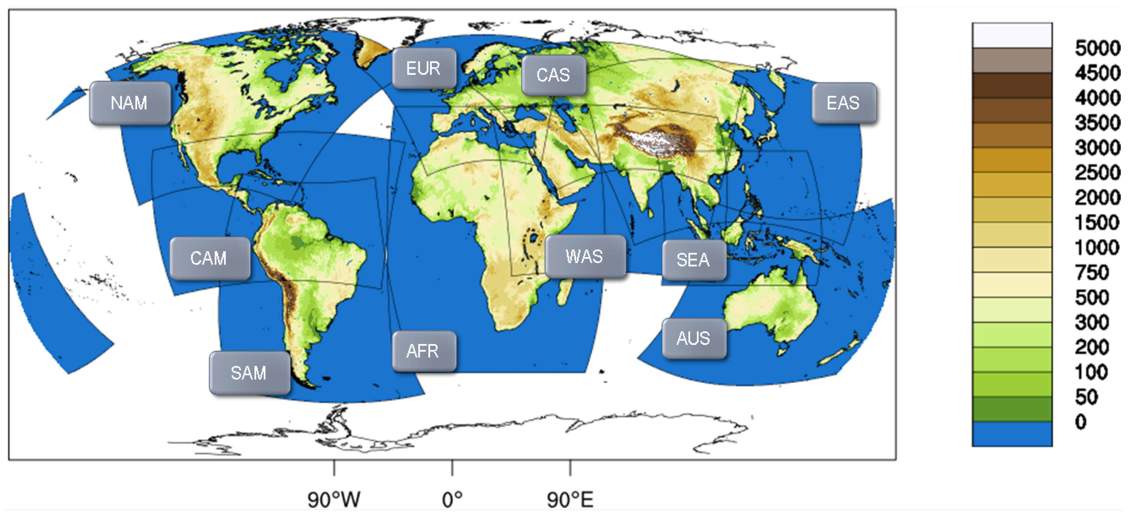
2.1. REMO
2.2. Köppen–Trewartha Climate Classification
2.3. Climate Statistics, Biases and Skill
3. Results
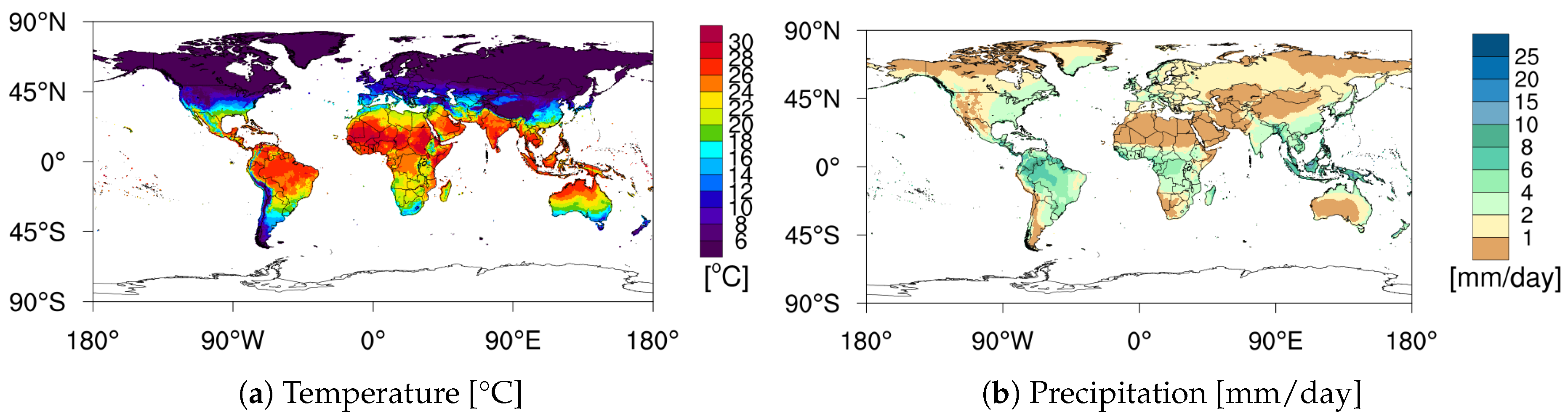
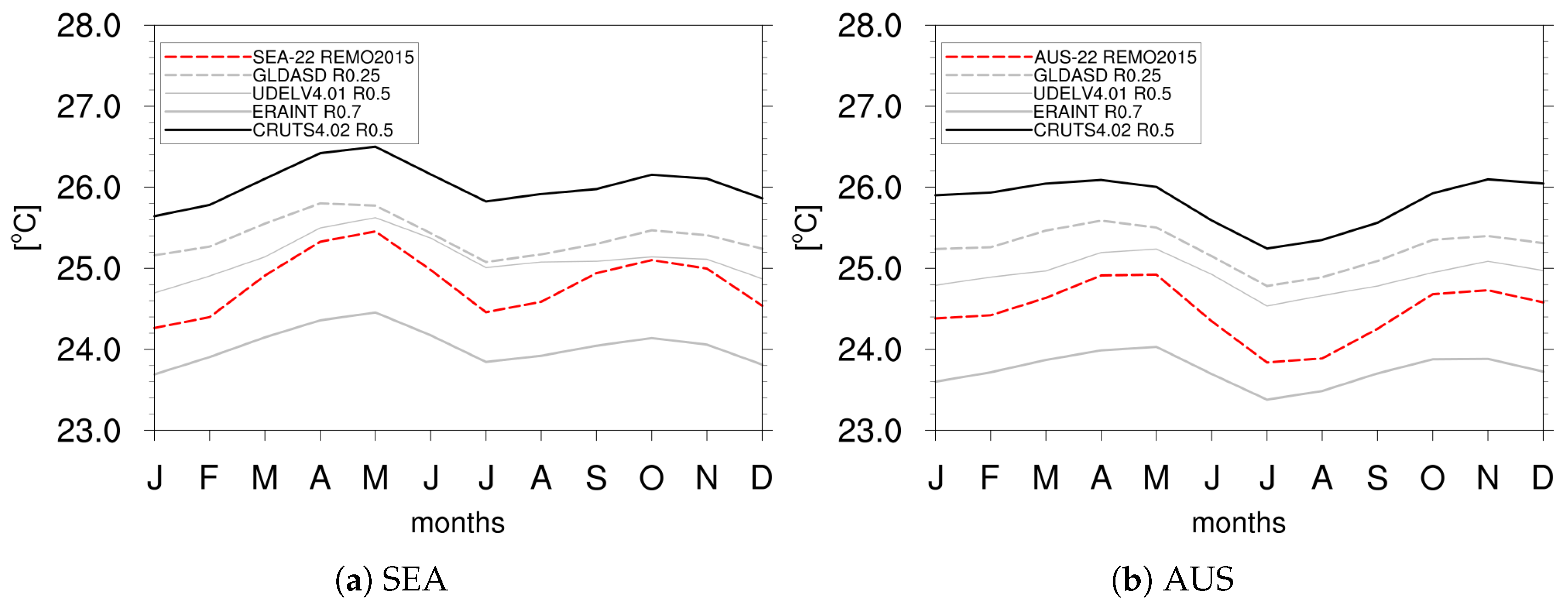
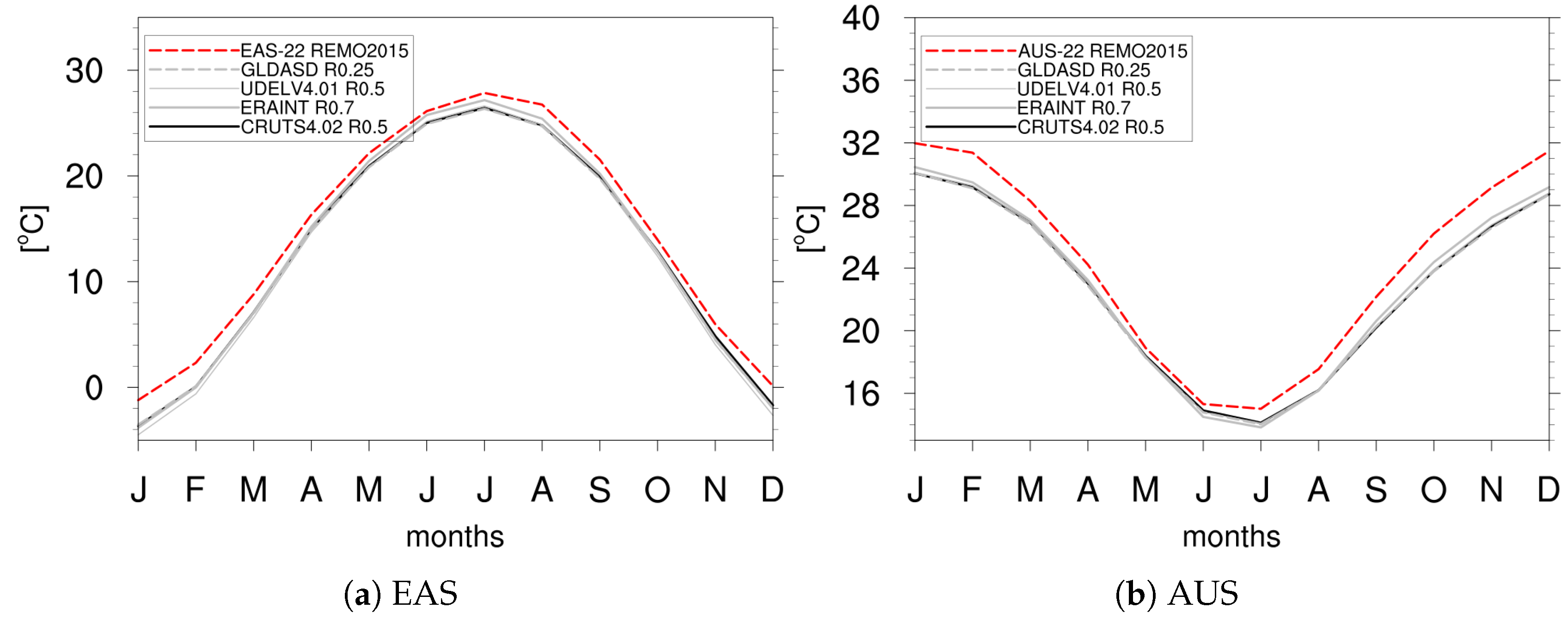
3.1. Temperature and Precipitation from Observations and Simulations
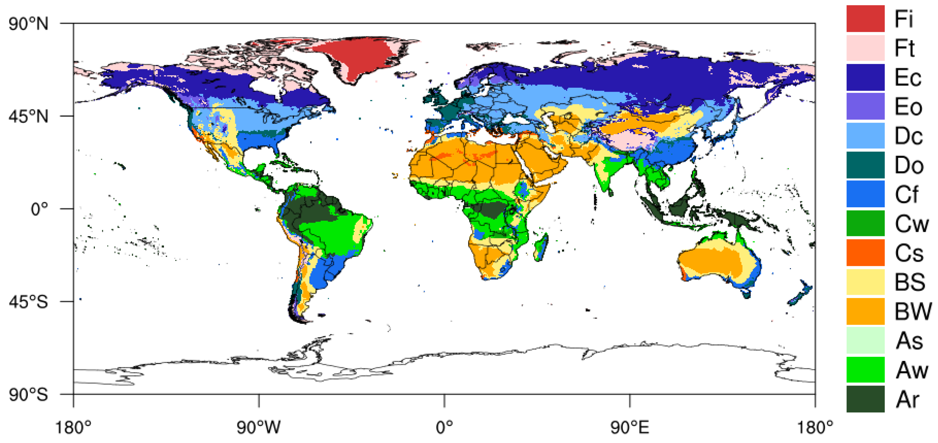
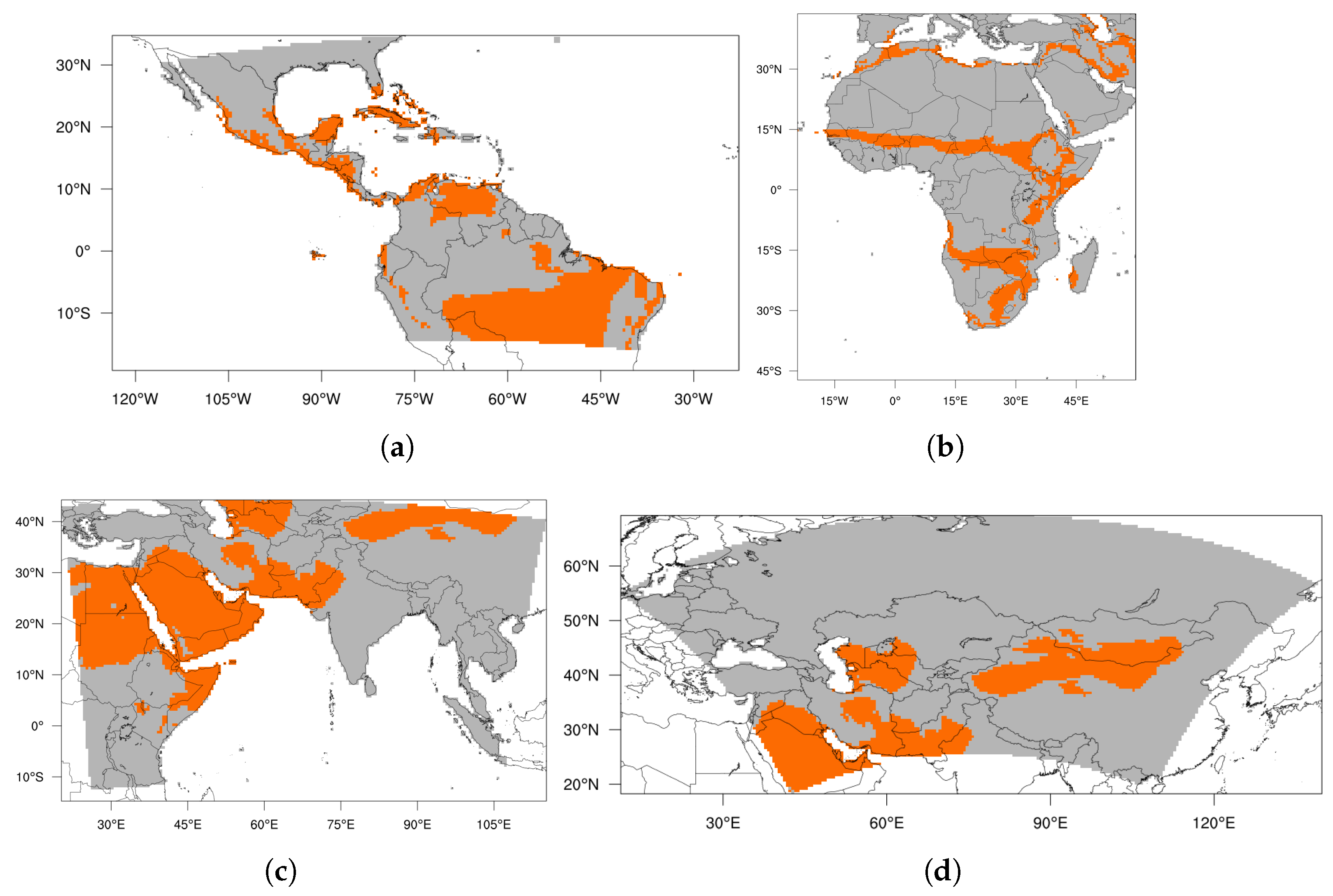
3.2. Derived Climate Regions
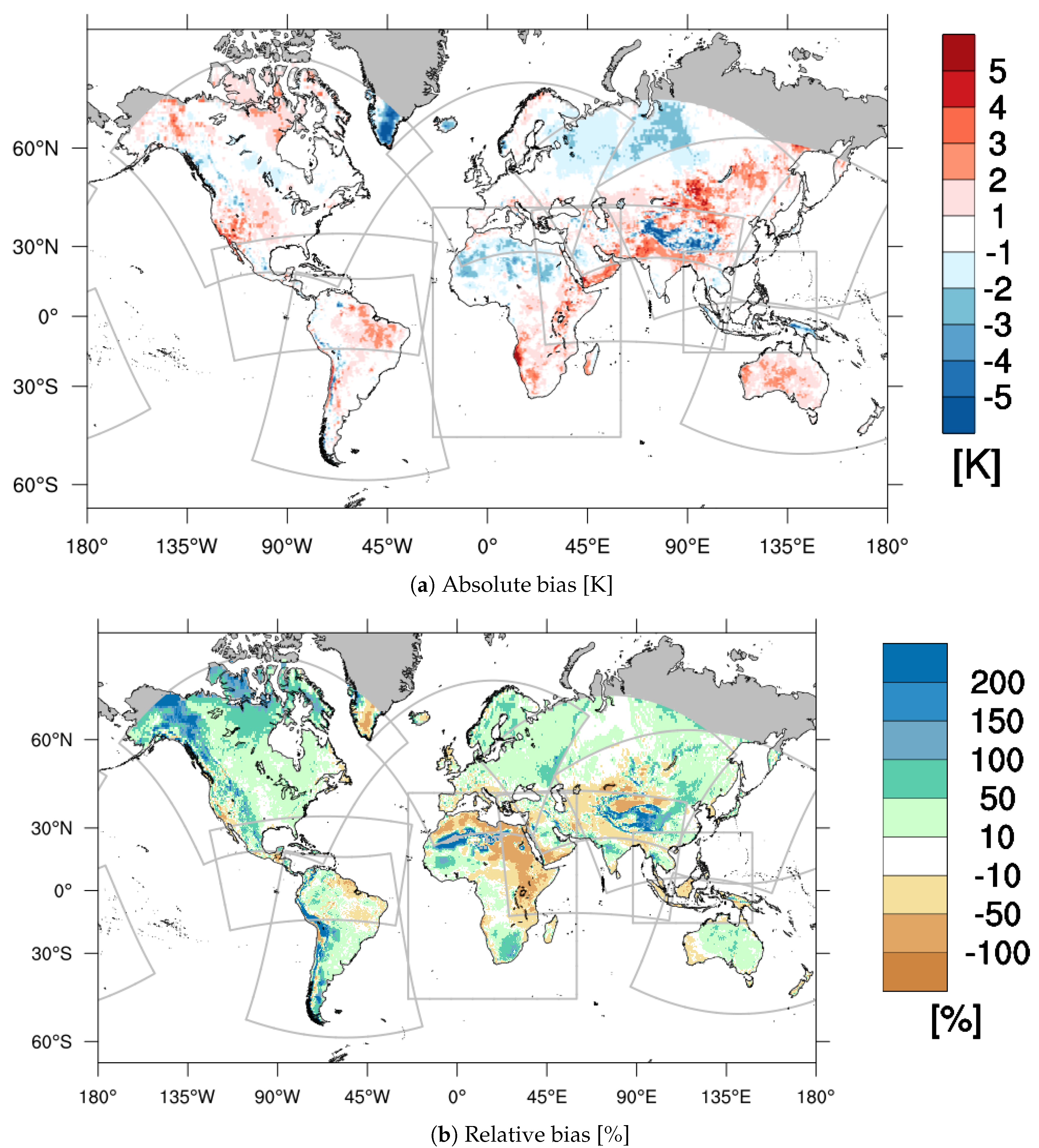
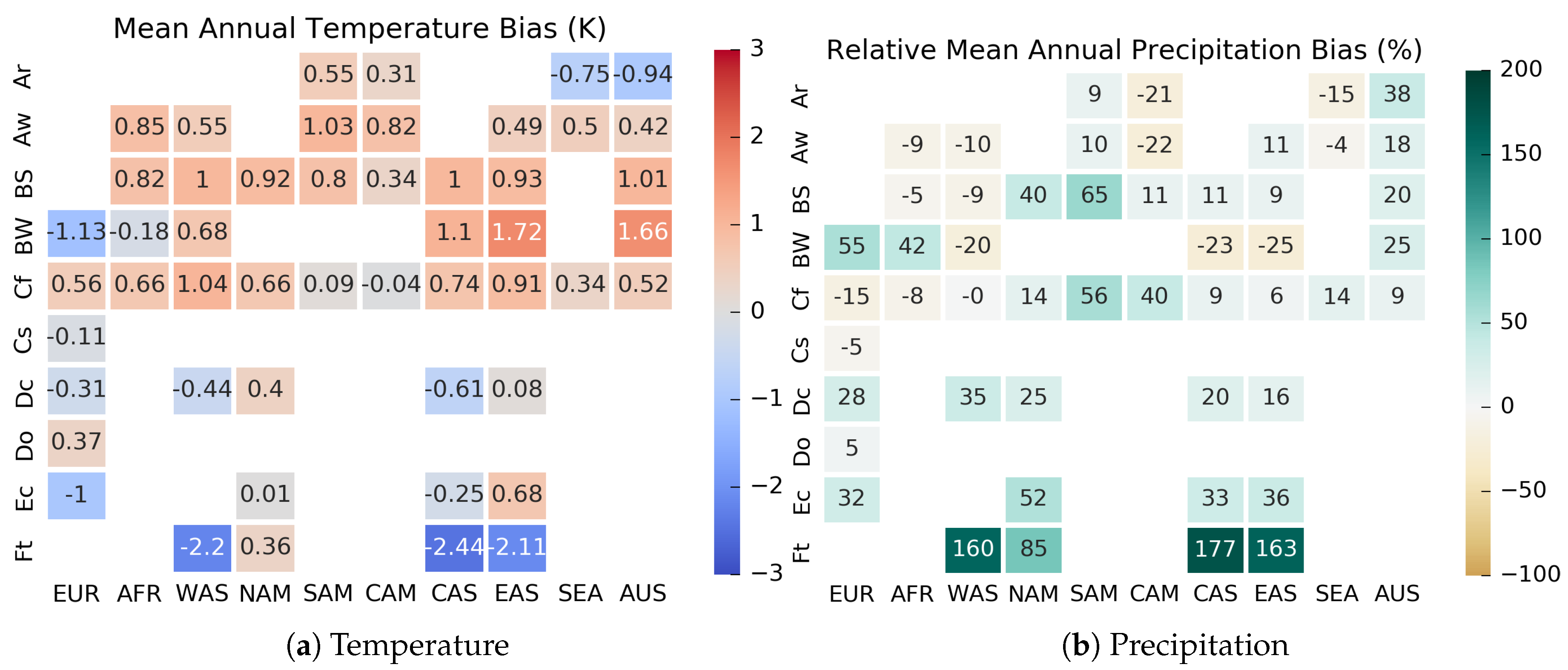
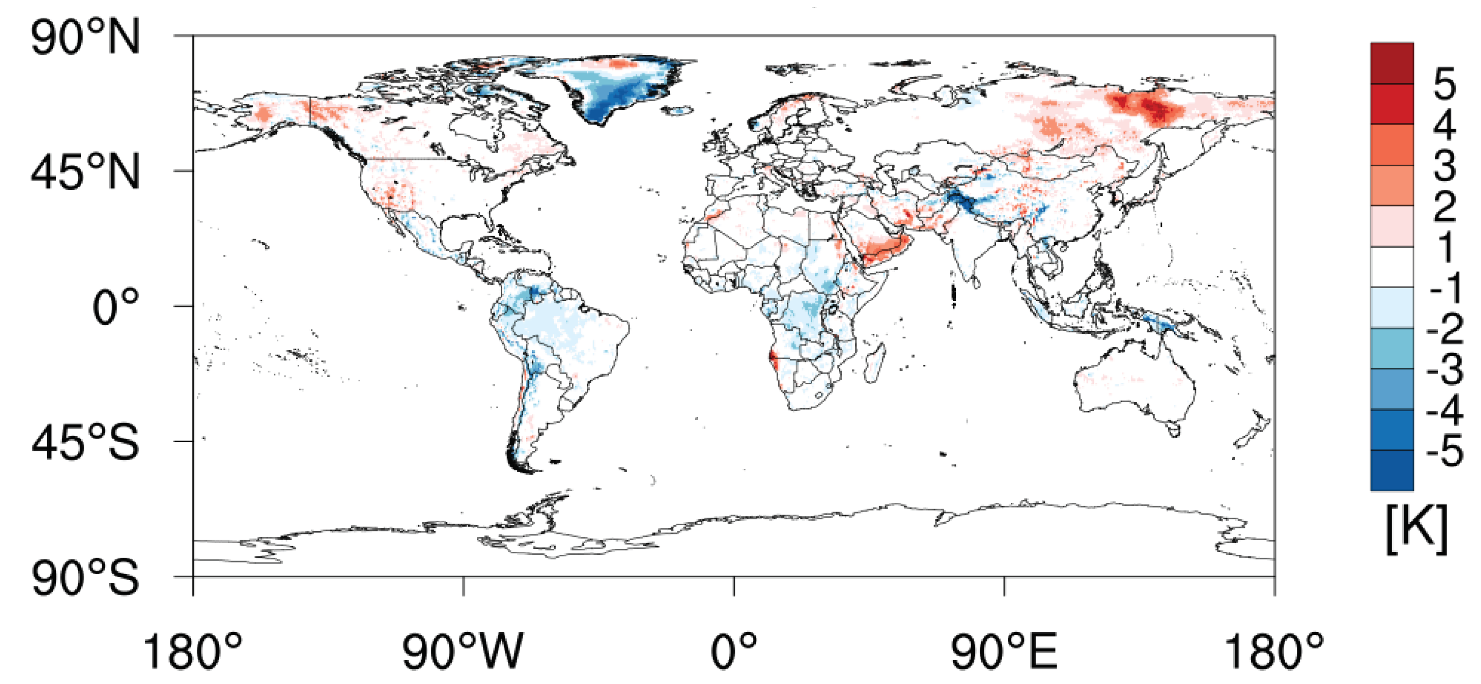
3.3. Mean Annual Biases Using the K–T Climate Types
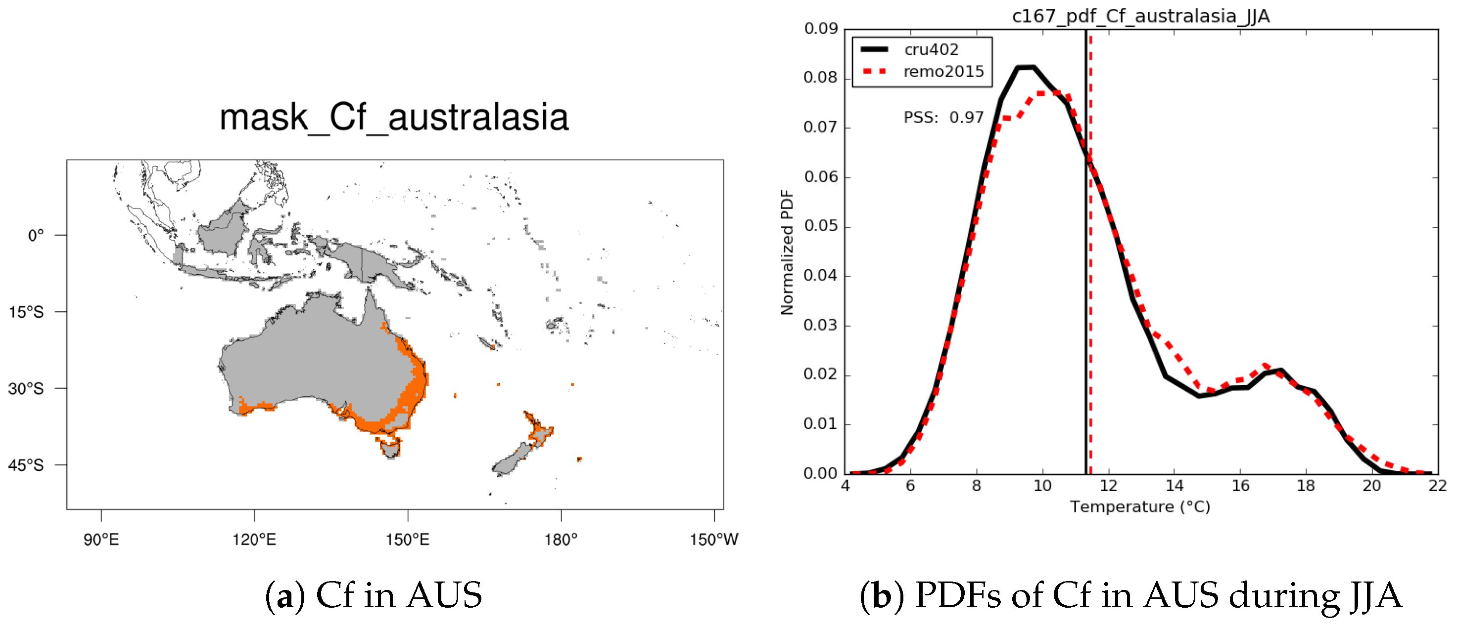
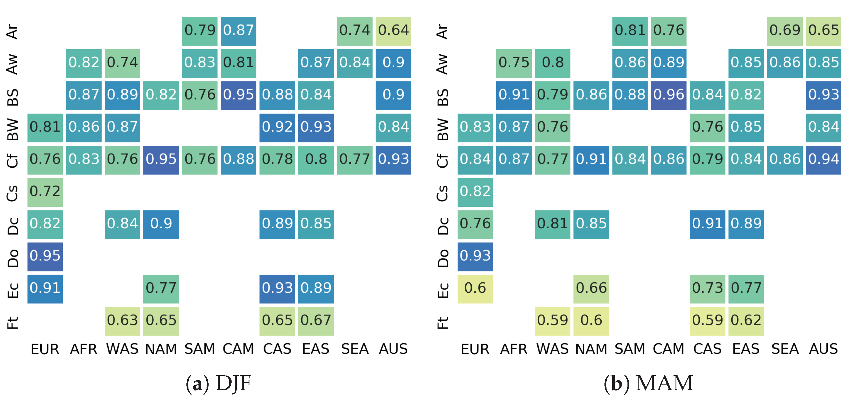
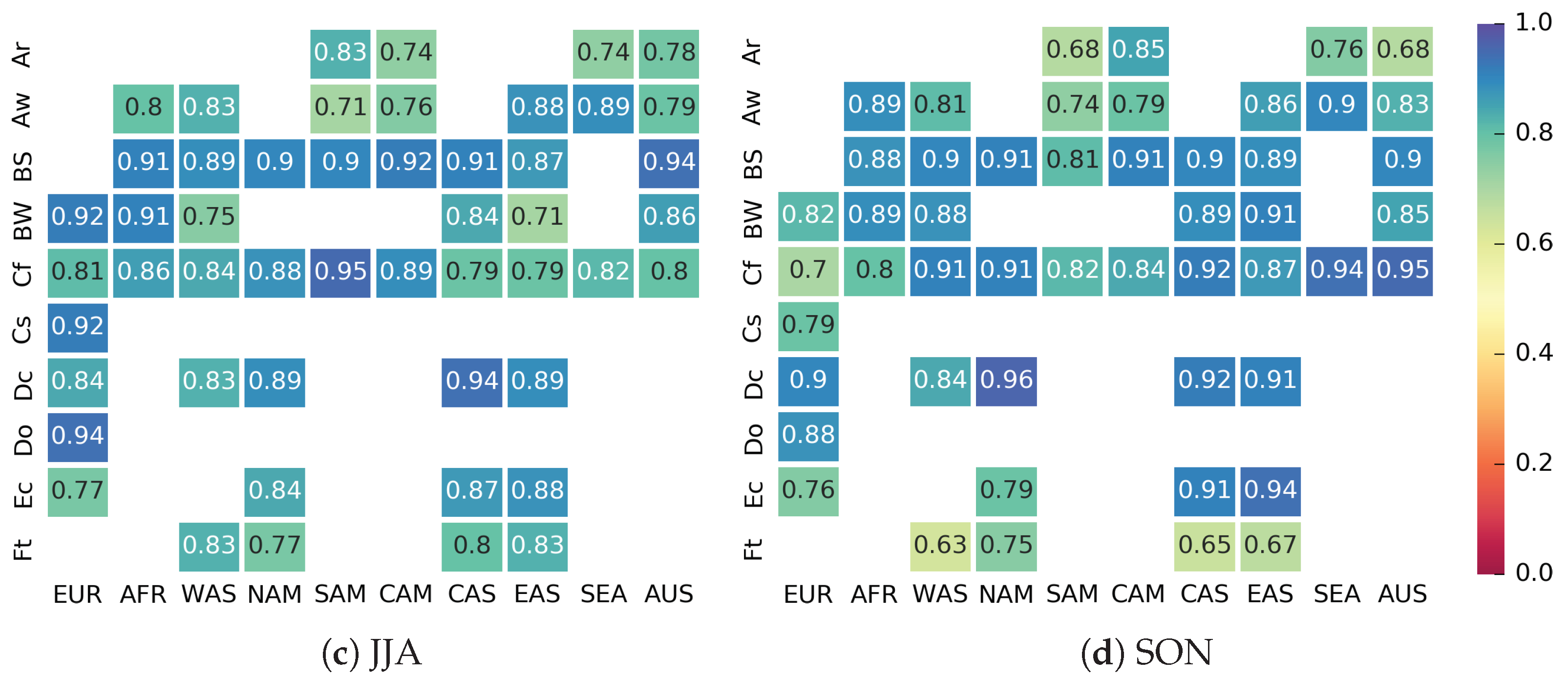
3.4. PDF Skill Score
4. Discussion
4.1. Tropical Climates
4.2. Dry Climates
4.3. Subtropical Climates
4.4. Temperate Climates
4.5. Sub-Arctic or Boreal Climates
4.6. Polar Climates
5. Conclusions
Author Contributions
Funding
Acknowledgments
Conflicts of Interest
References
- Giorgi, F.; Jones, C.; Asrar, G.R. Addressing climate information needs at the regional level: the CORDEX framework. Bull. World Meteorol. Org. 2009, 58, 175–183. [Google Scholar]
- Gutowski, J.W.; Giorgi, F.; Timbal, B.; Frigon, A.; Jacob, D.; Kang, H.S.; Raghavan, K.; Lee, B.; Lennard, C.; Nikulin, G.; et al. WCRP COordinated Regional Downscaling EXperiment (CORDEX): A diagnostic MIP for CMIP6. Geosci. Model Dev. 2016, 9, 4087–4095. [Google Scholar] [CrossRef]
- Dee, D.P.; Uppala, S.M.; Simmons, A.J.; Berrisford, P.; Poli, P.; Kobayashi, S.; Andrae, U.; Balmaseda, M.A.; Balsamo, G.; Bauer, P.; et al. The ERA-Interim reanalysis: Configuration and performance of the data assimilation system. Q. J. R. Meteorol. Soc. 2011, 137, 553–597. [Google Scholar] [CrossRef]
- van Vuuren, D.P.; Edmonds, J.; Kainuma, M.; Riahi, K.; Thomson, A.; Hibbard, K.; Hurtt, G.C.; Kram, T.; Krey, V.; Lamarque, J.F.; et al. The representative concentration pathways: An overview. Clim. Chang. 2011, 109, 5. [Google Scholar] [CrossRef]
- Haensler, A.; Hagemann, S.; Jacob, D. Dynamical downscaling of ERA40 reanalysis data over southern Africa: Added value in the simulation of the seasonal rainfall characteristics. Int. J. Climatol. 2011, 31, 2338–2349. [Google Scholar] [CrossRef]
- Haensler, A.; Hagemann, S.; Jacob, D. The role of the simulation setup in a long-term high-resolution climate change projection for the southern African region. Theor. Appl. Climatol. 2011, 106, 153–169. [Google Scholar] [CrossRef]
- Solman, S.A.; Sanchez, E.; Samuelsson, P.; da Rocha, R.P.; Li, L.; Marengo, J.; Pessacg, N.L.; Remedio, A.R.C.; Chou, S.C.; Berbery, H.; et al. Evaluation of an ensemble of regional climate model simulations over South America driven by the ERA-Interim reanalysis: Model performance and uncertainties. Clim. Dyn. 2013, 41, 1139–1157. [Google Scholar] [CrossRef]
- Kumar, P.; Podzun, R.; Hagemann, S.; Jacob, D. Impact of modified soil thermal characteristic on the simulated monsoon climate over south Asia. J. Earth Syst. Sci. 2014, 123, 151–160. [Google Scholar] [CrossRef]
- Cerezo-Mota, R.; Cavazos, T.; Arritt, R.; Torres-Alavez, A.; Sieck, K.; Nikulin, G.; Moufouma-Okia, W.; Salinas-Prieto, J.A. CORDEX-NA: Factors inducing dry/wet years on the North American Monsoon region. Int. J. Climatol. 2016, 36, 824–836. [Google Scholar] [CrossRef]
- Weber, T.; Haensler, A.; Rechid, D.; Pfeifer, S.; Eggert, B.; Jacob, D. Analyzing Regional Climate Change in Africa in a 1.5, 2, and 3°C Global Warming World. Earth’s Future 2018, 6, 643–655. [Google Scholar] [CrossRef]
- Jacob, D.; Kotova, L.; Teichmann, C.; Sobolowski, S.P.; Vautard, R.; Donnelly, C.; Koutroulis, A.G.; Grillakis, M.G.; Tsanis, I.N.K.; Damm, A.; et al. Climate Impacts in Europe Under +1.5/degreeC Global Warming. Earth’s Future 2018, 6, 264–285. [Google Scholar] [CrossRef]
- CORDEX Scientific Advisory Team. The WCRP CORDEX Coordinated Output for Regional Evaluations (CORE) Experiment Guidelines. Available online: http://www.cordex.org/experiment-guidelines/cordex-core/ (accessed on 1 March 2019).
- Ngo-Duc, T.; Tangang, F.T.; Santisirisomboon, J.; Cruz, F.; Trinh-Tuan, L.; Nguyen-Xuan, T.; Phan-Van, T.; Juneng, L.; Narisma, G.; Singhruck, P.; et al. Performance evaluation of RegCM4 in simulating extreme rainfall and temperature indices over the CORDEX-Southeast Asia region. Int. J. Climatol. 2017, 37, 1634–1647. [Google Scholar] [CrossRef]
- Tangang, F.; Supari, S.; Chung, J.X.; Cruz, F.; Salimun, E.; Ngai, S.T.; Juneng, L.; Santisirisomboon, J.; Santisirisomboon, J.; Ngo-Duc, T.; et al. Future changes in annual precipitation extremes over Southeast Asia under global warming of 2 °C. APN Sci. Bull. 2018, 8, 6–11. [Google Scholar] [CrossRef]
- Jacob, D.; Petersen, J.; Eggert, B.; Alias, A.; Christensen, O.B.; Bouwer, L.M.; Braun, A.; Colette, A.; Déqué, M.; Georgievski, G.; et al. EURO-CORDEX: New high-resolution climate change projections for European impact research. Reg. Environ. Chang. 2014, 14, 563–578. [Google Scholar] [CrossRef]
- Ozturk, T.; Altinsoy, H.; Türkeş, M.; Kurnaz, M.L. Simulation of temperature and precipitation climatology for the Central Asia CORDEX domain using RegCM 4.0. Clim. Res. 2012, 52, 63–76. [Google Scholar] [CrossRef]
- Fuentes-Franco, R.; Coppola, E.; Giorgi, F.; Pavia, E.G.; Diro, G.T.; Graef, F. Inter-annual variability of precipitation over Southern Mexico and Central America and its relationship to sea surface temperature from a set of future proje ctions from CMIP5 GCMs and RegCM4 CORDEX simulations. Clim. Dyn. 2015, 45, 425–440. [Google Scholar] [CrossRef]
- Wegener-Köppen, E.; Thiede, J. (Eds.) Wladimir Köppen—Scholar for Life; Schweizerbart Science Publishers: Stuttgart, Germany, 2018. [Google Scholar]
- Trewartha, G.T. An Introduction to Weather and Climate; McGraw-Hill Book Company, Inc.: New York, NY, USA; London, UK, 1943. [Google Scholar]
- Trewartha, G.T.; Horn, L.H. An Introduction to Climate, 5th ed.; McGraw-Hill Series in Geography; McGraw-Hill Kogakusha Ltd.: Tokyo, Japan, 1980. [Google Scholar]
- Belda, M.; Holtanová, E.; Halenka, T.; Kalvová, J. Climate classification revisited: From Köppen to Trewartha. Clim. Res. 2014, 59, 1–13. [Google Scholar] [CrossRef]
- De Castro, M.; Gallardo, C.; Jylha, K.; Tuomenvirta, H. The use of a climate-type classification for assessing climate change effects in Europe from an ensemble of nine regional climate models. Clim. Chang. 2007, 81, 329–341. [Google Scholar] [CrossRef]
- Jacob, D.; Elizalde, A.; Haensler, A.; Hagemann, S.; Kumar, P.; Podzun, R.; Rechid, D.; Remedio, A.R.; Saeed, F.; Sieck, K.; et al. Assessing the Transferability of the Regional Climate Model REMO to Different COordinated Regional Climate Downscaling EXperiment (CORDEX) Regions. Atmosphere 2012, 3, 181–199. [Google Scholar] [CrossRef]
- Fernandez, J.P.; Franchito, S.H.; Rao, V.B.; Llopart, M. Changes in Koppen–Trewartha climate classification over South America from RegCM4 projections. Atmos. Sci. Lett. 2017, 18, 427–434. [Google Scholar] [CrossRef]
- Baker, B.; Diaz, H.; Hargrove, W.; Hoffman, F. Use of the Köppen-Trewartha climate classification to evaluate climatic refugia in statistically derived ecoregions for the People’s Republic of China. Clim. Chang. 2009, 98, 113–131. [Google Scholar] [CrossRef]
- Schoetter, R.; Hoffmann, P.; Rechid, D.; Schlünzen, K.H. Evaluation and Bias Correction of Regional Climate Model Results Using Model Evaluation Measures. J. Appl. Meteorol. Climatol. 2012, 51, 1670–1684. [Google Scholar] [CrossRef]
- Annamalai, H.; Taguchi, B.; McCreary, J.P.; Nagura, M.; Miyama, T. Systematic Errors in South Asian Monsoon Simulation: Importance of Equatorial Indian Ocean Processes. J. Clim. 2017, 30, 8159–8178. [Google Scholar] [CrossRef]
- Kotlarski, S.; Keuler, K.; Christensen, O.B.; Colette, A.; Déqué, M.; Gobiet, A.; Goergen, K.; Jacob, D.; Lüthi, D.; van Meijgaard, E.; et al. Regional climate modeling on European scales: A joint standard evaluation of the EURO-CORDEX RCM ensemble. Geosci. Model Dev. 2014, 7, 1297–1333. [Google Scholar] [CrossRef]
- Nikulin, G.; Jones, C.; Giorgi, F.; Asrar, G.; Büchner, M.; Cerezo-Mota, R.; Christensen, O.B.; Déqué, M.; Fernandez, J.; Hänsler, A.; et al. Precipitation Climatology in an Ensemble of CORDEX-Africa Regional Climate Simulations. J. Clim. 2012, 25, 6057–6078. [Google Scholar] [CrossRef]
- Ambrizzi, T.; Reboita, M.S.; da Rocha, R.P.; Llopart, M. The state of the art and fundamental aspects of regional climate modeling in South America. Ann. N. Y. Acad. Sci. 2019, 1436, 98–120. [Google Scholar] [CrossRef]
- Perkins, S.E.; Pitman, A.J.; Holbrook, N.J.; McAneney, J. Evaluation of the AR4 Climate Models’ Simulated Daily Maximum Temperature, Minimum Temperature, and Precipitation over Australia Using Probability Density Functions. J. Clim. 2007, 20, 4356–4376. [Google Scholar] [CrossRef]
- Jacob, D.; Podzun, R. Sensitivity studies with the regional climate model REMO. Meteorol. Atmos. Phys. 1997, 63, 119–129. [Google Scholar] [CrossRef]
- Jacob, D.; Van Den Hurk, B.J.; Andræ, U.; Elgered, G.; Fortelius, C.; Graham, L.P.; Jackson, S.D.; Karstens, U.; Köpken, C.; Lindau, R.; et al. A comprehensive model inter-comparison study investigating the water budget during the BALTEX-PIDCAP period. Meteorol. Atmos. Phys. 2001, 77, 19–43. [Google Scholar] [CrossRef]
- Roeckner, E.; Arpe, K.; Bengtsson, L.; Christoph, M.; Claussen, M.; Dümenil, L.; Esch, M.; Giorgetta, M.; Schlese, U.; Schulzweida, U. The atmospheric general circulation model ECHAM-4: Model description and simulation of present-day climate. MPI Rep. 1996, 218, 171. [Google Scholar]
- Majewski, D. The Europa–Modell of the Deutscher Wetterdienst. In ECMWF Seminar on Numerical Methods in Atmospheric Models; ECMWF: Reading, UK, 1991; Volume 2, pp. 147–191. [Google Scholar]
- Pietikäinen, J.P.; O’Donnell, D.; Teichmann, C.; Karstens, U.; Pfeifer, S.; Kazil, J.; Podzun, R.; Fiedler, S.; Kokkola, H.; Birmili, W.; et al. The regional aerosol-climate model REMO-HAM. Geosci. Model Dev. 2012, 5, 1323–1339. [Google Scholar] [CrossRef]
- Pietikäinen, J.P.; Markkanen, T.; Sieck, K.; Jacob, D.; Korhonen, J.; Räisänen, P.; Gao, Y.; Ahola, J.; Korhonen, H.; Laaksonen, A.; et al. The regional climate model REMO (v2015) coupled with the 1D freshwater lake model FLake (v1): Fenno-Scandinavian climate and lakes. Geosci. Model Dev. 2018, 11, 1321–1342. [Google Scholar] [CrossRef]
- Wilhelm, C.; Rechid, D.; Jacob, D. Interactive coupling of regional atmosphere with biosphere in the new generation regional climate system model REMO-iMOVE. Geosci. Model Dev. 2014, 7, 1093–1114. [Google Scholar] [CrossRef]
- Sein, D.V.; Mikolajewicz, U.; Gröger, M.; Fast, I.; Cabos, W.; Pinto, J.G.; Hagemann, S.; Semmler, T.; Izquierdo, A.; Jacob, D. Regionally coupled atmosphere-ocean-sea ice-marine biogeochemistry model ROM: 1. Description and validation. J. Adv. Model. Earth Syst. 2015, 7, 268–304. [Google Scholar] [CrossRef]
- Tiedtke, M. A Comprehensive Mass Flux Scheme for Cumulus Parameterization in Large-Scale Models. Mon. Weather Rev. 1989, 117, 1779–1800. [Google Scholar] [CrossRef]
- Nordeng, T.E. Extended Versions of the Convective Parametrization Scheme at ECMWF and Their Impact on the Mean and Transient Activity of the Model in the Tropics; Technical Report; ECMWF Research Department, European Centre for Medium Range Weather Forecast: Reading, UK, 1994. [Google Scholar]
- Pfeifer, S. Modeling Cold Cloud Processes with the Regional Climate Model REMO. Ph.D. Thesis, University of Hamburg, Hamburg, Germany, 2006. [Google Scholar]
- Lohmann, U.; Roeckner, E. Design and performance of a new cloud microphysics scheme developed for the ECHAM4 general circulation model. Clim. Dyn. 1996, 12, 557–572. [Google Scholar] [CrossRef]
- Morcrette, J.J.; Smith, L.; Fouquart, Y. Pressure and temperature dependence of the absorption in longwave radiation parameterizations. Beitraege Phys. Atmos. 1986, 59, 455–469. [Google Scholar]
- Giorgetta, M.; Wild, M. The Water Vapour Continuum and Its Representation in ECHAM4; Technical Report; Max-Planck Institut für Meteorologie Report No. 162; Max Planck Institute for Meteorology: Hamburg, Germany, 1995. [Google Scholar]
- Tanre, D.; Geleyn, J.F.; Slingo, J.M. First, results of the introduction of an advanced aerosol-radiation interaction in the ECMWF low resolution global model. In Aerosols and their Climatic Effects; Deepak Publ.: Hampton, Virginia, 1984; pp. 133–177. [Google Scholar]
- Louis, J.F. A Parametric Model Of Vertical Eddy Fluxes In The Atmosphere. Bound. Layer Meteorol. 1979, 17, 187–202. [Google Scholar] [CrossRef]
- Hagemann, S. An Improved Land Surface Parameter Dataset for Global and Regional Climate Models; Report 336; Max-Planck-Institute for Meteorology: Hamburg, Germany, 2002. [Google Scholar]
- Kotlarski, S. A Subgrid Glacier Parameterisation for Use in Regional Climate Modelling. Ph.D. Thesis, University of Hamburg, Hamburg, Germany, 2007. [Google Scholar]
- Rechid, D.; Jacob, D. Influence of monthly varying vegetation on the simulated climate in Europe. Meteorol. Z. 2006, 15, 99–116. [Google Scholar] [CrossRef]
- Rechid, D.; Raddatz, T.J.; Jacob, D. Parameterization of snow-free land surface albedo as a function of vegetation phenology based on MODIS data and applied in climate modelling. Theor. Appl. Climatol. 2009, 95, 245–255. [Google Scholar] [CrossRef]
- Charnock, H. Wind stress on water: An hypothesis. Q. J. R. Meteorol. Soc. 1955, 81, 639–640. [Google Scholar] [CrossRef]
- Kumar, P.; Wiltshire, A.; Mathison, C.; Asharaf, S.; Ahrens, B.; Lucas-Picher, P.; Christensen, J.H.; Gobiet, A.; Saeed, F.; Hagemann, S.; et al. Downscaled climate change projections with uncertainty assessment over India using a high resolution multi-model approach. Sci. Total Environ. 2013, 468-469, S18–S30. [Google Scholar] [CrossRef] [PubMed]
- Remedio, A.R.C. Connections of Low Level Jets and Mesoscale Convective Systems in South America. Ph.D. Thesis, University of Hamburg, Hamburg, Germany, 2013. [Google Scholar]
- Davies, H.C. A lateral boundary formulation for multi-level prediction models. Quart. J. Roy. Meteor. Soc. 1976, 102, 405–418. [Google Scholar] [CrossRef]
- Harris, I.; Jones, P.D.; Osborn, T.J.; Lister, D.H. Updated high-resolution grids of monthly climatic observations—The CRU TS3.10 Dataset. Int. J. Climatol. 2014, 34, 623–642. [Google Scholar] [CrossRef]
- Teichmann, C.; Eggert, B.; Elizalde, A.; Haensler, A.; Jacob, D.; Kumar, P.; Moseley, C.; Pfeifer, S.; Rechid, D.; Remedio, A.; et al. How Does a Regional Climate Model Modify the Projected Climate Change Signal of the Driving GCM: A Study over Different CORDEX Regions Using REMO. Atmosphere 2013, 4, 214–236. [Google Scholar] [CrossRef]
- Max Planck Institute for Meteorology. Climate Data Operators. Available online: http://code.zmaw.de/projects/cdo (accessed on 6 October 2018).
- Schamm, K.; Ziese, M.; Becker, A.; Finger, P.; Meyer-Christoffer, A.; Schneider, U.; Schröder, M.; Stender, P. Global gridded precipitation over land: A description of the new GPCC First, Guess Daily product. Earth Syst. Sci. Data 2014, 6, 49–60. [Google Scholar] [CrossRef]
- Legates, D.R.; Willmott, C.J. Mean seasonal and spatial variability in global surface air temperature. Theor. Appl. Climatol. 1990, 41, 11–21. [Google Scholar] [CrossRef]
- Legates, D.R.; Willmott, C.J. Mean seasonal and spatial variability in gauge-corrected, global precipitation. Int. J. Climatol. 1990, 10, 111–127. [Google Scholar] [CrossRef]
- Rodell, M.; Houser, P.R.; Jambor, U.; Gottschalck, J.; Mitchell, K.; Meng, C.J.; Arsenault, K.; Cosgrove, B.; Radakovich, J.; Bosilovich, M.; et al. The Global Land Data Assimilation System. Bull. Am. Meteorol. Soc. 2004, 85, 381–394. [Google Scholar] [CrossRef]
- Di Virgilio, G.; Evans, J.P.; Di Luca, A.; Olson, R.; Argüeso, D.; Kala, J.; Andrys, J.; Hoffmann, P.; Katzfey, J.J.; Rockel, B. Evaluating reanalysis-driven CORDEX regional climate models over Australia: model performance and errors. Clim. Dyn. 2019, 1–21. [Google Scholar] [CrossRef]
- Razuvaev, V.; Apasova, E.; Martuganov, R.; Vose, R.; Steurer, P. Daily Temperature and Precipitation Data for 223 USSR Stations; Technical Report; Oak Ridge National Laboratory (ORNL): Oak Ridge, TN, USA, 1993. [Google Scholar] [CrossRef]
- Eggert, B. Auswirkungen der Oberflächeneigenschaften in REMO auf die Simulation der unteren Atmosphäre; Technical Report; Climate Service Center Germany, Helmholtz-Zentrum Geesthacht: Hamburg, Germany, 2011. [Google Scholar]
- Demaria, E.M.C.; Rodriguez, D.A.; Ebert, E.E.; Salio, P.; Su, F.; Valdes, J.B. Evaluation of mesoscale convective systems in South America using multiple satellite products and an object-based approach. J. Geophys. Res. Atmos. 2011, 116. [Google Scholar] [CrossRef]
- Jones, D.A.; Wang, W.; Fawcett, R. High-quality spatial climate data-sets for Australia. Aust. Meteorol. Oceanogr. J. 2009, 58, 233–248. [Google Scholar] [CrossRef]
- Solmon, F.; Mallet, M.; Elguindi, N.; Giorgi, F.; Zakey, A.; Konaré, A. Dust aerosol impact on regional precipitation over western Africa, mechanisms and sensitivity to absorption properties. Geophys. Res. Lett. 2008, 35. [Google Scholar] [CrossRef]
- Zhao, T.; Fu, C. Comparison of products from ERA-40, NCEP-2, and CRU with station data for summer precipitation over China. Adv. Atmos. Sci. 2006, 23, 593–604. [Google Scholar] [CrossRef]
- Prein, A.F.; Gobiet, A. Impacts of uncertainties in European gridded precipitation observations on regional climate analysis. Int. J. Climatol. 2017, 37, 305–327. [Google Scholar] [CrossRef]
- Schneider, U.; Becker, A.; Finger, P.; Meyer-Christoffer, A.; Ziese, M.; Rudolf, B. GPCC’s new land surface precipitation climatology based on quality-controlled in situ data and its role in quantifying the global water cycle. Theor. Appl. Climatol. 2014, 115, 15–40. [Google Scholar] [CrossRef]


| Parameters | EUR | AFR | WAS | NAM | SAM | CAM | CAS | EAS | SEA | AUS |
|---|---|---|---|---|---|---|---|---|---|---|
| x | 241 | 401 | 401 | 321 | 301 | 433 | 325 | 433 | 288 | 433 |
| y | 217 | 433 | 271 | 271 | 361 | 241 | 217 | 271 | 217 | 271 |
| ZDLAND-L | 7500 | 20,000 | 25,000 | 7500 | 7500 | 25,000 | 25,000 | 25,000 | 25,000 | 7500 |
| ZDLAND-O | 7500 | 15,000 | 30,000 | 7500 | 7500 | 30,000 | 30,000 | 30,000 | 30,000 | 7500 |
| CHAR | 0.0123 | 0.0123 | 0.00123 | 0.0123 | 0.0123 | 0.0123 | 0.0123 | 0.0123 | 0.0123 | 0.0123 |
| Types | Description |
|---|---|
| A: Tropical climates; > 18 C; ≥ R | |
| Ar | humid; 10 to 12 months wet; 0 to 2 months dry |
| Aw | Winter (low-sun period) dry; > 2 months dry |
| As | Summer (high-sun period) dry; rare climate type |
| B: Dry climates; | |
| BS | semi-arid; |
| BW | arid; < |
| C: Subtropical climates; < 18 C | |
| Cs | summer-dry; at least 3× as much rain in winter as in summer; |
| < 3 cm; < 89 cm | |
| Cw | summer-wet; winter dry; |
| at least 10x as much rain in summer as in winter | |
| Cf | humid; No dry season; difference between driest and wettest month |
| less than required for Cs and Cw; > 3 cm | |
| D: Temperate climates; 4 to 7 months with > 10 C | |
| Do | oceanic; > 0 C |
| Dc | continental; ≤ 0 C |
| E: Sub-arctic or boreal climates; | |
| 1 to 3 months with > 10 C | |
| Eo | oceanic; > −10 C |
| Ec | continental; ≤ −10 C |
| F: Polar climates; < 10 C | |
| Ft | Tundra/Highland; > 0 C |
| Fi | Ice cap; ≤ 0 C |
| Domains | CRU Mean | Temporal STD | REMO Bias | Spatial STD |
|---|---|---|---|---|
| EUR | 11.32 | −0.40 | ||
| NAM | 4.35 | +0.34 | ||
| AFR | 23.14 | +0.29 | ||
| SAM | 22.01 | +0.63 | ||
| WAS | 19.21 | +0.36 | ||
| CAM | 24.32 | +0.48 | ||
| CAS | 6.96 | +0.01 | ||
| EAS | 9.18 | +0.51 | ||
| SEA | 23.15 | +0.03 | ||
| AUS | 22.79 | +0.90 |
| Domains | CRU Mean | Temporal STD | REMO Bias | Spatial STD | Rel Bias | Rel Spatial STD |
|---|---|---|---|---|---|---|
| EUR | 1.50 | +0.22 | +26.11 | |||
| NAM | 1.85 | +0.50 | +40.29 | |||
| AFR | 1.62 | +0.85 | +15.92 | |||
| SAM | 4.28 | −0.08 | +40.40 | |||
| WAS | 1.91 | +0.05 | +7.43 | |||
| CAM | 4.74 | −0.78 | −7.35 | |||
| CAS | 1.25 | +0.28 | +23.62 | |||
| EAS | 2.04 | +0.34 | +24.93 | |||
| SEA | 5.32 | −0.36 | −0.30 | |||
| AUS | 3.39 | +0.64 | +22.44 |
| Types | “WORLD” | EUR | AFR | WAS | NAM | SAM | CAM | CAS | EAS | SEA | AUS |
|---|---|---|---|---|---|---|---|---|---|---|---|
| Ar | 8.7 | - | 4.34 | 4.94 | 1.00 | 28.37 | 36.03 | - | 2.89 | 44.50 | 27.09 |
| As | 0.1 | - | 0.05 | 0.02 | - | 0.27 | 0.33 | - | 0.02 | - | - |
| Aw | 13.1 | - | 19.29 | 15.64 | 2.53 | 33.88 | 36.69 | 0.20 | 9.72 | 29.42 | 8.72 |
| BS | 12.7 | 4.74 | 16.96 | 15.42 | 10.31 | 10.21 | 10.45 | 13.71 | 14.82 | 1.31 | 21.65 |
| BW | 18.1 | 18.92 | 43.32 | 33.75 | 3.66 | 4.84 | 4.81 | 19.22 | 12.78 | - | 28.62 |
| Cf | 8.2 | 6.58 | 5.69 | 9.31 | 8.31 | 13.85 | 10.76 | 6.21 | 12.61 | 22.58 | 9.74 |
| Cs | 1.4 | 6.12 | 4.08 | 2.14 | 0.89 | 0.64 | 0.12 | 0.91 | 0.01 | - | 1.07 |
| Cw | 0.5 | - | 1.24 | 1.12 | - | 0.04 | - | 0.49 | 0.74 | 0.51 | - |
| Dc | 11.4 | 31.97 | 2.64 | 5.89 | 25.21 | 0.01 | - | 24.47 | 16.53 | 0.18 | 0.05 |
| Do | 3.5 | 15.44 | 2.29 | 3.10 | 4.65 | 2.59 | 0.04 | 3.01 | 2.46 | 1.36 | 2.73 |
| Ec | 13.4 | 10.83 | 0.07 | 1.81 | 25.15 | - | - | 24.98 | 19.18 | - | - |
| Eo | 1.6 | 4.09 | - | 0.86 | 3.67 | 1.81 | 0.08 | 0.97 | 1.26 | 0.06 | 0.30 |
| Fi | 1.0 | - | - | - | 0.77 | - | - | - | - | - | - |
| Ft | 6.2 | 1.30 | 0.02 | 6.00 | 13.85 | 3.47 | 0.70 | 5.84 | 6.98 | 0.09 | 0.02 |
| Total land area | |||||||||||
| (× 10 km) | 146 | 16 | 40 | 32 | 23 | 19 | 15 | 35 | 30 | 9 | 13 |
© 2019 by the authors. Licensee MDPI, Basel, Switzerland. This article is an open access article distributed under the terms and conditions of the Creative Commons Attribution (CC BY) license (http://creativecommons.org/licenses/by/4.0/).
Share and Cite
Remedio, A.R.; Teichmann, C.; Buntemeyer, L.; Sieck, K.; Weber, T.; Rechid, D.; Hoffmann, P.; Nam, C.; Kotova, L.; Jacob, D. Evaluation of New CORDEX Simulations Using an Updated Köppen–Trewartha Climate Classification. Atmosphere 2019, 10, 726. https://doi.org/10.3390/atmos10110726
Remedio AR, Teichmann C, Buntemeyer L, Sieck K, Weber T, Rechid D, Hoffmann P, Nam C, Kotova L, Jacob D. Evaluation of New CORDEX Simulations Using an Updated Köppen–Trewartha Climate Classification. Atmosphere. 2019; 10(11):726. https://doi.org/10.3390/atmos10110726
Chicago/Turabian StyleRemedio, Armelle Reca, Claas Teichmann, Lars Buntemeyer, Kevin Sieck, Torsten Weber, Diana Rechid, Peter Hoffmann, Christine Nam, Lola Kotova, and Daniela Jacob. 2019. "Evaluation of New CORDEX Simulations Using an Updated Köppen–Trewartha Climate Classification" Atmosphere 10, no. 11: 726. https://doi.org/10.3390/atmos10110726
APA StyleRemedio, A. R., Teichmann, C., Buntemeyer, L., Sieck, K., Weber, T., Rechid, D., Hoffmann, P., Nam, C., Kotova, L., & Jacob, D. (2019). Evaluation of New CORDEX Simulations Using an Updated Köppen–Trewartha Climate Classification. Atmosphere, 10(11), 726. https://doi.org/10.3390/atmos10110726