Area-Averaged Surface Moisture Flux over Fragmented Sea Ice: Floe Size Distribution Effects and the Associated Convection Structure within the Atmospheric Boundary Layer

Abstract

Sea ice fragmentation results in the transformation of the surface from relatively homogeneous to highly heterogeneous. Atmospheric boundary layer (ABL) rapidly responds to those changes through a range of processes which are poorly understood and not parametrized in numerical weather prediction (NWP) models. The aim of this work is to increase our understanding and develop parametrization of the ABL response to different floe size distributions (FSD). The analysis is based on the results of simulations with the Weather Research and Forecasting model. Results show that FSD determines the distribution and intensity of convection within the ABL through its influence on the atmospheric circulation. Substantial differences between various FSDs are found in the analysis of spatial arrangement and strength of ABL convection. To incorporate those sub-grid effects in the NWP models, a correction factor for the calculation of surface moisture heat flux is developed. It is expressed as a function of floe size, sea ice concentration and wind speed, and enables a correction of the flux computed from area-averaged quantities, as is typically done in NWP models. In general, the presented study sheds some more light on the sea ice–atmosphere interactions and provides the first attempt to parametrize the influence of FSD on the ABL.

1. Introduction

Parametrization of sub-mesoscale processes related to spatially heterogeneous land/water surface remains one of the key challenges in atmosphere and climate modeling. In polar regions, sea ice surface properties vary over a wide range of scales, from centimeters to tens of kilometers, influencing the oceanic and atmospheric boundary layers through many complex interactions. The quality of weather and climate predictions depends heavily on our ability to accurately represent the effects of those interactions in numerical weather prediction (NWP) models. As most of currently used climate models have horizontal grid spacing of tens of kilometers and are therefore unable to directly reproduce processes related to smaller-scale sea ice features, their effects must be parametrized. However, the scarcity of observations of atmospheric properties over fragmented sea ice and the resulting incomplete understanding of the sub-mesoscale processes hampers the development of parametrizations. Consequently, sub-grid interactions between the surface and the atmosphere, which may account for the inaccuracies present in model predictions [1,2], are poorly represented in NWP models.

The influence of sea ice heterogeneity on the atmospheric boundary layer (ABL) has long been the subject of both modeling [3,4,5,6] and observational studies [7,8,9,10]. The general aspects of ABL’s response to the presence of open water areas in the form of singular or several leads in an otherwise continuous ice cover are relatively well studied. These effects include changes of the ABL stability over and downstream of open leads [5,8], sensitivity to prevailing wind conditions [10,11], formation of steam fog and cloud plumes [12], or initiation of gravity waves [4]. Similarly, the influence of leads width on the strength of the atmospheric response has been studied as well [13,14], and it is generally assumed that for a given total surface area of leads, numerous narrow leads tend to induce stronger area-averaged turbulent exchange of heat and moisture than a few wide ones. However, recent satellite data studies indicate that such conclusion might be flawed [15] and suggest that the larger contribution from small leads to the total surface heat flux may not be associated with their efficiency, but rather number density, length and frequency of their occurrence in the Arctic. Other studies point out that not only the average lead width is important, but also their spatial arrangement and the shape of their size distribution [16]. According to modeling results [17,18], even very small open water areas might result in the development of small convective plumes which penetrate the ABL and modify its circulation and properties. The areas of updraft air motion can be recognized in the winter Arctic from the satellites due to the presence of steam fog. Steam fog occurs because of cold ($-40{}^{\circ }$C to $-5{}^{\circ }$C) air advection over water which is only slightly warmer than its freezing point. The fog is characterized by either columnar or banded structure and extends in height from 1 to 1500 meters with the liquid water content in the range of 0.01–0.5 g/m${}^3$ [19]. This fog type can be recognized in satellite images as linear features, organized into bands of different width, interspersed with clear air areas [20], or as plume-like streaks, with a typical spacing of a few kilometers [21]. Numerical studies indicate that such features may have significant impact on atmospheric processes not only locally, but also regionally [5,18,22].

Obviously, large scale models do not directly resolve heterogeneity at scales smaller than the model grid cell. To account for the larger-scale effects of sub-grid properties of the atmosphere and the underlying surface, NWP models must rely on estimation methods and simplified parametrizations. Computation of surface turbulent heat fluxes (STHF)—the main subject of the present paper—provides a very good example of problems associated with constructing such parametrizations. Locally, STHF is a function of several variables characterizing the surface and the lower atmosphere (temperature, wind speed, etc.). Due to the nonlinear character of the relationship between those variables and spatial correlations between them, the area-averaged STHF cannot be directly computed from the area-averaged variables, available in numerical models. The necessary correction depends on the characteristics of the surface (size and spatial arrangement of “patches” of different surface types; in the case of ice-covered sea surface analyzed here: spatial distribution of sea ice and open water) and the associated local response of the lower atmosphere. Several approaches to this problem have been developed and are used in various NWP models.

In the standard, most basic approach, a single, dominant type of the surface in a grid cell is used as representative for that cell. Thus, the cell-averaged surface fluxes are calculated from cell-averaged atmospheric and surface properties, like, e.g., in the standard version of COSMO-CLM or CCLm model [23]. Such averaging of atmospheric and surface properties is termed an “aggregation” process. An important disadvantage of this approach is a possibility that the aggregation will produce biased results due to the above-mentioned nonlinear relationship between the variables involved. The problem of biased STHF estimates has long been recognized [14,24,25,26] and several improved methods of flux calculation have been proposed. One of the most popular ones is a so-called mosaic method developed by Avissar and Pielke [27]. In this approach, the sub-grid variability is accounted for by independently coupling each surface type within a grid cell to the overlying atmosphere. Surface-specific fluxes are thus calculated from area-averaged atmospheric properties (as previously), but with the consideration of the parameters specific for each surface type. Grid cell-averaged fluxes are then obtained by summing the fluxes from different surfaces, weighted by the fractional area they cover. This method has been adopted, sometimes with slight modifications, in various modeling [26,28,29] and observational [30] studies. The mosaic approach, to some extent, includes the effects of surface heterogeneity, but due to very complex relationship between the ABL and the underlying surface, it represents only a rough estimation of surface–atmosphere interactions, completely disregarding spatial structure of those interactions. As we demonstrate in this work, in the case of ABL over fragmented sea ice it is that spatial structure that is responsible for large deviations between area-averaged fluxes computed with different methods. It is very likely that in the case of winter sea ice fragmentation, the averaging of atmospheric variables is behind the largest errors in NWP predictions of STHF. This is because differences between local ABL properties over sea ice and open water are often very large (e.g., can reach even tens of degrees in the case of air temperature).

The methods of STHF calculation described above rely solely on sea ice concentration in a grid cell and do not take into account any information about spatial arrangement of ice and water within that cell (size of ice floes, presence and orientation of leads and fractures, etc.). This limitation seems particularly serious in view of the present climate change in the polar regions, associated with a rapid transition of the sea ice cover, with decreasing extent of multiyear sea ice and expanding proportion of seasonal ice [31]. Due to the fact that seasonal, first-year sea ice is more prone to breaking and deformation due to external forcing, heterogeneous sea ice is going to appear more frequently [32]. Since the sea ice cover moderates energy transfer between ocean and atmosphere and is highly sensitive to weather patterns changes, the atmospheric response to sea ice fragmentation becomes a particularly important research topic. A specific aspect related to sea ice fragmentation that attracted a lot of scientific attention throughout the years is the floe size distribution (FSD), defined as the number of floes in different size categories in a given region, divided by the area of that region [33]. It is a key parameter in describing the state of the marginal ice zone (MIZ) and the evolution of sea ice cover. The information about floe size is essential to determine the rate of lateral sea ice melt [34], to assess the sea ice dynamics and internal stresses [35], and to resolve sea ice interactions with oceanic [36] and atmospheric boundary layers [17]. The importance of FSD drives the effort to include its representation into sea ice and climate models. Equations describing the evolution of the joint distribution of sea ice thickness and floe size were formulated and implemented in a continuum sea ice model by Horvat and Tziperman [37]. The advantage of this model, further developed by Roach et al. [38], is that it does not involve any assumptions about the form of that distribution, so that it is allowed to evolve in response to forcing from the ocean and atmosphere. Another approach, alternative to continuum models, is based on discrete-element methods (DEM), as, e.g., by Herman [39] whose joint-particle DEM allows direct simulations of floe formation due to dynamic processes. However, due to extremely high computational costs of DEMs, larger-scale sea ice simulations must be based on continuum models (coupled with atmospheric, oceanic and possibly other components). The new possibility of including FSD in those models, described above, provides a wide range of possibilities in terms of implementing new physical processes, both influencing and influenced by the FSD. On the other hand, however, this can be done only if those processes are sufficiently well understood. In the case of the response of the ABL to sea ice fragmentation, this is at present not the case. Moreover, observations that could contribute to improving our knowledge are very rare if not non-existent. Therefore, in order to implement FSD-related effects into NWP models we should first focus on better understanding of its impact on the atmospheric and oceanic boundary layers and the physical processes involved, in parallel with the development of parametrizations that would make the models less expensive computationally.

Several aspects of the ABL response to sea ice heterogeneity have been studied thoroughly in the recent numerical study of Wenta and Herman [17]. They examined the influence of small-scale sea ice surface variability (different floe size distributions or different lead widths and orientation) on domain-averaged STHF and properties of the ABL (e.g., the total moisture content). In agreement with earlier studies, mentioned above, the model predicted formation of convective plumes, rapid release of heat and moisture, strong local wind speed increase and intensification of vertical air motions. Crucially for the present analysis, at the same ice concentration, different size and spatial arrangement of ice floes resulted in changes of the domain-averaged ABL properties. This indicates that the above-described methods of computing STHF, based solely on sea ice concentration, might produce biased results, with inaccuracy dependent on the properties of FSD. Furthermore, significant correlation is observed not only between the local surface and atmospheric variables, but also within the ABL itself (i.e., between ABL properties at different heights), indicating that the transfer coefficients used in the STHF algorithms should take into account local variations of temperature and wind speed.

In this study, the influence of FSD on the ABL is studied further. The modeling results obtained by Wenta and Herman [17] are examined, with the focus on the convective structures within the ABL and the surface turbulent moisture heat flux (the second component of STHF, the sensible heat flux, will be analyzed in a subsequent study). The goal of the first part of the analysis (Section 3.1) is to explain how the spatial arrangement and size of convective structures depends on the floe size distribution, and to describe the properties of those structures found in the modeling results. (Anticipating Section 3.1, it is important to stress here that convection cells in this case do not have characteristic, regular shapes typical for Rayleigh–Benard convection, and therefore they are referred to as convective structures rather than convective cells in the rest of this paper.) The convection analysis is also used to explain the variability of domain-averaged STHF and total cloud liquid water content found in Wenta and Herman [17].

The goal of the research described in the second part of the paper (Section 3.2) is to develop a formula that would allow incorporating the FSD-related effects in the calculation of surface turbulent moisture heat flux (further referred as surface moisture heat flux, or SMHF). More specifically, the goal is to propose a correction factor, dependent on floe size, which might be used in combination with the existing, ice-concentration-based flux formulae in order to improve their accuracy over fragmented sea ice. The proposed correction takes a form of a coefficient, denoted with $\alpha$, which describes the ratio between the surface moisture flux $F_m$ calculated with two different methods: $\alpha =F_{m,1}/F_{m,2}$. In the first method, the effects of FSD are properly accounted for as the surface and atmospheric quantities on the sub-grid scale are taken directly from high-resolution numerical simulations. In the second method, the flux is determined with one of the algorithms described earlier, i.e., it is based on area-averaged properties of the surface and the atmosphere. Obviously, the computation of $F_{m,2}$ depends on the availability of surface and atmospheric properties present in a given atmospheric model. As described in detail in Section 3.2, $\alpha$ can be formulated as a function of area-averaged wind speed, ice concentration and floe size, so that, for given ice and wind conditions, $F_{m,2}$ can be computed in a traditional way and corrected for FSD effects by multiplying it with $\alpha$.

It must be stressed that the proposed correction is based on idealized modeling results and must be validated with observations and further modeling in the future. Therefore, it can be understood as the first step towards a parametrization suitable for implementation in NWP models.

2. Methods

2.1. Configuration of the WRF Model

Results from the modeling study of Wenta and Herman [17] are used in the analysis in the present study. This section provides a brief description of the model configuration and initial conditions; detailed information can be found in [17].

The Advanced Research Weather Research and Forecasting (ARW WRF) model is used in an “idealized mode”. In this approach, the model is initialized with a single sounding file consisting of the vertical profiles of potential temperature, water vapor mixing ratio, and the two components of wind velocity. The full air pressure and density, as well as other atmospheric variables, are initialized from that input sounding. The model domain is rectangular, with periodic boundaries in both horizontal directions, dimensions 200 × 200 grid points and horizontal resolution of 100 m, thus covering the area of 20,000 × 20,000 m. The top boundary is set at 2000 m above the surface, close to the top of the inversion layer separating the ABL from the free atmosphere in the initial sounding. At the upper model boundary, a damping zone is defined as a Rayleigh relaxation layer of 200 m depth, with a default damping coefficient of 0.002 s${}^{-1}$. The vertical velocity component at the top of the model domain is set to zero. Air column is divided into 61 vertical levels with exponential thickness distribution, from ∼2 m at the surface to ∼200 m at the top. Each simulation used in this analysis was performed for 14 h, with a time step of 1 s. The results were stored every 10 min.

The parametrization schemes of physical processes along with diffusion options are chosen based on the WRF model validation performed in other studies under similar conditions (

Table A1. WRF model configuration used in the analysis described in the present paper.

Model Domain	Rectangular, periodic boundaries in both horizontal directions
Horizontal resolution	100 m
Number of grid points	200 × 200
Model top height	2000 m
Air column	61 $\eta$-levels with exponential thickness distribution
	Physics Parametrizations
Microphysics	WRF Single-Moment 5-class scheme
Longwave radiation	RRTMG Scheme
Surface layer	Eta Similarity Scheme
Land Layer	Noah Land Surface Model
Large-eddy simulation	1.5-order TKE scheme
	Sea Ice Options
Sea ice in a grid cell	Treats sea ice as fractional field.
Maximum allowed snow accumulation on sea ice	10${}^{10}$ m
Minimum allowed accumulation of snow on sea ice	0.001 m
Default sea ice thickness	1.5 m

). A detailed description of selected settings together with the justification of their choice can be found in [17].

The model box is placed at 75${}^{\circ }$ N, 160${}^{\circ }$ E, i.e., at the location of the Surface Heat Budget of The Arctic Ocean (SHEBA) experiment [40]. The Coriolis parameter, corresponding to that latitude, is assumed constant and equal to $1.417\times {10}^{-4}$ s${}^{-1}$. We assume, for simplicity, that at the start of each simulation the wind blows from west to east. For each sea ice mask (see below), the simulations are run 6 times: with wind speed equal to zero, and for 5 different wind speed profiles obtained by modifying the profile measured during SHEBA on 23rd of February 1998 (see [17] for details). The resulting vertically averaged values of wind speed for initial profiles 1–5 are as follows: 1.06 m/s, 2.1 m/s, 4.26 m/s, 7.4 m/s and 9.35 m/s, respectively.

The surface water temperature is set to freezing point, assumed equal to 271.4 K. The initial temperature within sea ice varies linearly from 271.4 K at the bottom to the air temperature at the upper ice surface. Default roughness length values are used, equal to $1\times {10}^{-4}$ m over water and $1\times {10}^{-3}$ m over ice.

In the present study, six different sea ice concentration values are considered: $c=50$%, $c=60$%, $c=70$%, $c=80$%, $c=85$% and $c=90$%. For each ice concentration and wind speed profile, the model is launched for a series of simulations with different spatial arrangements of ice floes. Sea ice is represented as round floes with a power-law probability distribution of their radii $P(r)\sim r^{-\beta }$, with an exponent $\beta =1.8$ (values between 1.5 and 2.0 are typically observed in the marginal ice zone). Floe radii range from several tens of meters to over 4 km. The sea ice masks for WRF are obtained by first generating an ensemble of floes with a desired total ice surface area, corresponding to a prescribed c and number of floes $N_f$; subsequently, these floes are randomly placed within a temporary, very large rectangular domain at a very low ice concentration and without floe overlap, and a DEM model [39] is used to reduce the size of that domain and to obtain the final floe positions, from which eventually an ice concentration map is computed. In other words, the DEM is used to converge the initially loosely packed floe assemblage to obtain a desired ice concentration—which is otherwise a rather nontrivial task. A summary of all floe configurations considered is given in Wenta and Herman [17].

To summarize, in the analysis presented below we consider simulations which are initialized with five different floe-size distributions, six wind profiles and six sea ice concentrations, giving a total of 180 combinations. Different FSDs are distinguished in the first part of the analysis by $N_f$, but in the calculation of the $\alpha$ coefficient a median of floe radius is calculated for every FSD in order to make the algorithm applicable in other studies (obviously, $N_f$ is domain-size dependent).

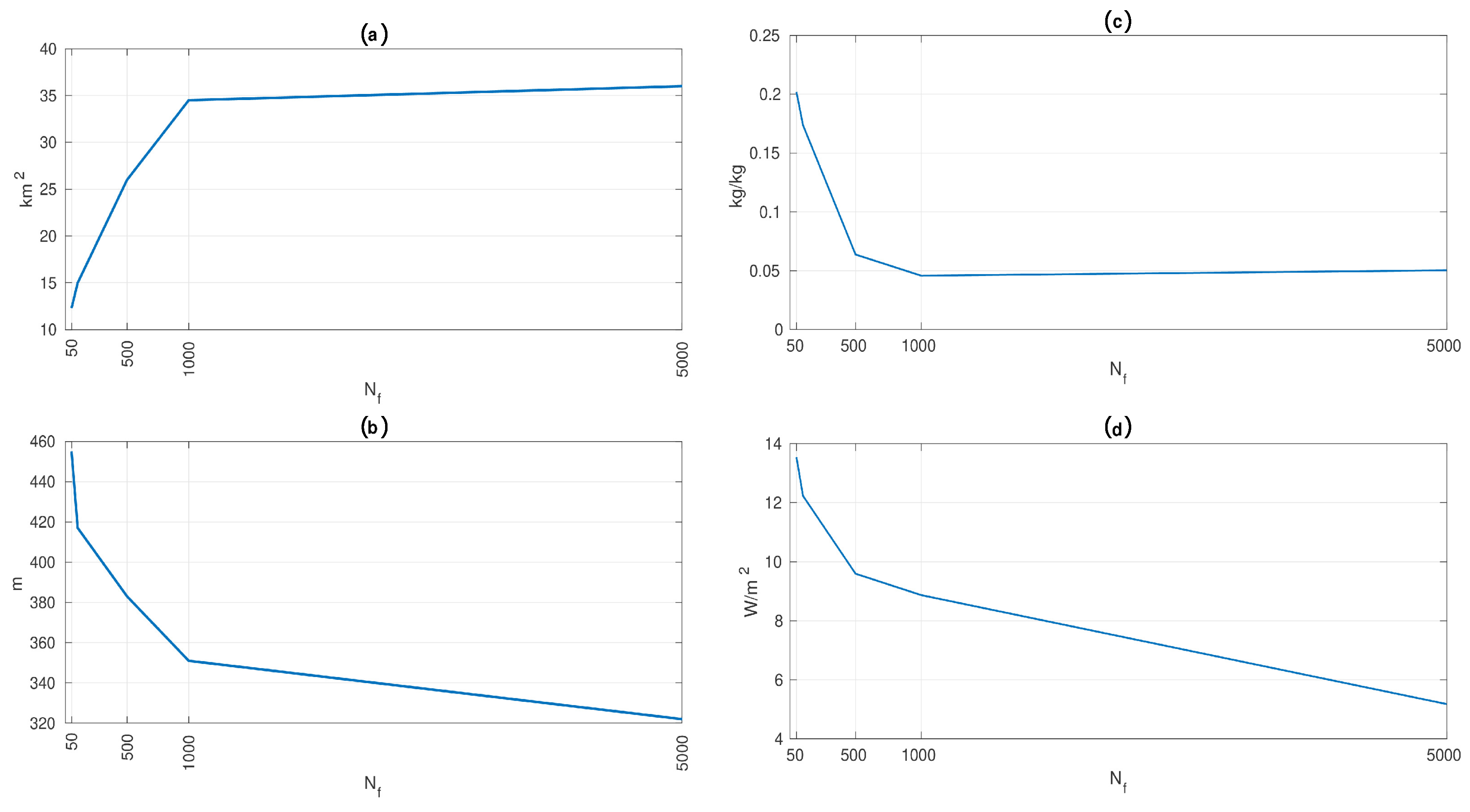
2.2. Calculation of Spatial Coverage of Convective Structures

The study of convective structures within the model domain is based on the analysis of the vertical component of the air motion. The highest values of turbulent fluxes, water vapor and cloud liquid content within the atmosphere are associated with positive (upward) values of vertical wind component, which in the present context serve as an indicator of convective motion. In the first step of the analysis, gray-colored maps of upward air motion areas are generated for every output time step of a given simulation (Figure 1a). In the next step, the program called Pixie is used to determine the size of updraft areas in every produced image. Pixie was created specifically for the presented research and is available for free on GitLab (https://gitlab.com/seadata-software/pixie). It is a Python script that applies simple methods of image recognition to distinguish the areas of upward air motion. It processes every image and counts the pixels for a given color intensity threshold from 0 (black) to 255 (white). For the presented study, a 140 threshold has been determined as the most suitable and applied for the whole analysis (Figure 1b). Based on the computed number of classified pixels and the number of pixels present in the whole model domain, the total updraft area in km${}^2$ and their fractional coverage is computed.

2.3. Computation of Area-Averaged Surface Moisture Heat Flux

In the WRF model, the latent turbulent heat flux is obtained as a product of the moisture heat flux and the specific latent heat for vaporization of water; therefore, our study of surface moisture flux and the method of its adjustment due to sea ice fragmentation can also be applied to the latent heat flux.

The surface variables in the WRF setup described in Section 2.1 are calculated using the parametrization by Janjić [41], Janić [42]. In this high-resolution WRF application, where the planetary boundary layer schemes are turned off, the upward moisture flux $F_m$ (kg m${}^{-2}$s${}^{-1}$) at the surface is given as:

$$F_m={\rho }_a{C}_h(q_a-q_{z_0}),$$

(1)

where ${\rho }_a$ (kg/m${}^3$) is air density, $C_h$ (m/s) denotes the surface exchange coefficient for heat, $q_a$ (kg/kg) is water vapor mixing ratio at the lowest layer of the atmosphere, and $q_{z_0}$ (kg/kg) denotes specific humidity at roughness length. The surface turbulent exchange coefficient for heat is computed using Monin–Obukhov similarity theory [43]:

$$C_h=\frac{k{u}^{\ast }}{[ln(\frac{z}{z_{0m}})-{\psi }_m\frac{z}{L}][ln(\frac{z}{z_{0t}})-{\psi }_h\frac{z}{L}]},$$

(2)

where k is von Kármán constant, $u^{\ast }$ (m/s) is a friction velocity, z (m) is the height of the lowest model layer, $z_{0m}$ (m) is defined as a height at and below which the mean wind speed becomes zero, and $z_{0t}$ (m) denotes the height below which vertical transfer is through molecular diffusion and above which mixing by air currents dominates. L denotes the Monin–Obukhov length and ${\psi }_m$ and ${\psi }_h$ are integrated similarity functions for momentum and heat, respectively. Another surface related parameter $q_{z_0}$ is obtained from:

$$q_{z_0}=\frac{\frac{C_h{z}_q}{{\alpha }_t}(q_a+q_s)}{\frac{C_h{z}_q}{{\alpha }_t}+1}\mathrm{where}{\alpha }_t=2.1\times {10}^{-5},$$

(3)

with $z_q$ (m) symbolizing moisture roughness length, $q_s$ (kg/kg) specific humidity at lower boundary, and ${\alpha }_t$ (m${}^2$/s) the thermal diffusivity of air.

In the following analysis, the whole model domain of 20,000 × 20,000 m is treated as a single grid cell of an NWP model. Sub-grid variations of the relevant variables are obtained directly from the 40,000 grid points of 100 × 100 m dimensions, which together form the modeled area. As mentioned in the introduction, the correction coefficient $\alpha$ is defined as the ratio between moisture heat fluxes $F_{m,1}$ and $F_{m,2}$, which differ in terms of the order of averaging of surface and atmospheric properties:

$$\alpha =\frac{F_{m,1}}{F_{m,2}}.$$

(4)

To obtain the value of $F_{m,1}$, the moisture heat flux from Equation (1) is calculated for every grid point of the model domain. In the next step, it is area-averaged and it thus represents the “true” area-averaged moisture flux:

$$F_{m,1}=\overline{F_m}=\overline{{\rho }_a{C}_h(q_a-q_{z_0})}.$$

(5)

In the calculation of $F_{m,2}$, averaging takes place at the level of flux equations components, i.e., the values of ${\rho }_a$, $C_h$, $q_a$, and $q_{z_0}$ from every grid point are area-averaged over the model domain, and then used as input in the flux computation:

$$F_{m,2}=\overline{{\rho }_a}\overline{C_h}\left(\overline{q_a}-\overline{q_{z_0}}\right).$$

(6)

This approach corresponds to the aggregation method described in the introduction.

Another method of flux calculations, described as “mosaic” in the introduction, is also tested to determine whether similar patterns and relations are present. When this method is used in NWP models, the atmospheric properties are averaged over a grid cell area, but the surface quantities of $q_{z_0}$ and $C_h$ are computed by one-dimensional (1D) SVAT model driven by grid-scale atmospheric quantities [26]. In the present study, the sub-grid properties of the surface are taken directly from the high-resolution model results and averaged separately over sea ice and water (e.g., $\overline{C_{h,water}}$, $\overline{q_{z0,ice}}$, etc.). Therefore, the flux is calculated from the atmospheric quantities which are averaged over the whole model domain (as in the method above), and the surface quantities which are averaged over each surface type, and weighted with ice concentration:

$$F_{m,3}=(1-c)\overline{{\rho }_a}\overline{C_{h,water}}(\overline{q_a}-\overline{q_{z_0,water}})+c\overline{{\rho }_a}\overline{C_{h,ice}}(\overline{q_a}-\overline{q_{z_0,ice}}).$$

(7)

The corresponding correction coefficient in this case, analogous to Equation (4), is:

$$\gamma =\frac{F_{m,1}}{F_{m,3}}.$$

(8)

In all cases analyzed, the ratio between $F_{m1}$ and $F_{m3}$ is slightly smaller (by 0.1–0.3) than that between $F_{m1}$ and $F_{m2}$, but overall $\alpha$ and $\gamma$ follow the same pattern. It is found that the averaging of atmospheric properties is responsible for the largest errors in the calculation of moisture heat flux. Considering that this averaging is done in both methods, the further analysis is limited to the coefficient $\alpha$, due to the straightforwardness and simplicity of computation of the term in its denominator ($F_{m,2}$).

More than 180 values of $\alpha$ are obtained from simulations with 5 different FSDs, 6 initial wind speed profiles and 6 sea ice concentrations along with several additional tests with different initial conditions. As described in Section 2.1, the FSD is represented by the median floe radius in the model domain (r), and the spatial and temporal mean of wind speed $U_m$ is used to characterize wind conditions. For every combination of initial conditions, $\alpha$ is calculated for every output time step of a 14-h long simulation, and the median of those values is considered further. The aim of the analysis is to express $\alpha$ in terms of sea ice concentration, FSD and wind speed: $\alpha =\alpha (c,r,U_m)$.

3. Results

3.1. Horizontal and Vertical Structure of Convection

Convection found in our modeling results is driven by thermal instability, which develops when an open water area comes in contact with sufficiently cool air above. Open water areas of various sizes, scattered throughout the model domain, are locations of rapid exchange of heat and moisture. Convective plumes develop between sea ice floes and transform the atmospheric circulation in the whole ABL. Intensive turbulent exchange over open water rapidly warms the lowest atmospheric layer and produces negative pressure anomalies. The resulting pressure differences between sea ice floes and water produce a breeze-like circulation. In the weak wind conditions (wind profiles No. 1–3), a distinct pattern of the flow from the central parts of sea ice floes toward surrounding open water areas is present, while in simulations with stronger wind (wind profiles No. 3–5) it is a bit less distinguishable and dominated by intensive flow over open water. In general, over large floes the wind speed increases with the distance from their centers and is strongly enhanced over water, becoming the major factor behind strong updrafts and large values of turbulent fluxes in those areas (Figure 2).

The most conspicuous plumes occur roughly halfway between neighboring sea ice floes or at the edges of the floes. The strengthening of updraft occurs because over open water the breeze wind flow coming from one floe meets with the one from another floe creating a convergence zone. Most intensive plumes reach the height of 1000 m and are usually present over the largest open water regions, while the weakest ones penetrate the atmosphere only for dozens of meters and tend to be associated with narrow regions of open water between tightly packed sea ice floes. Altogether, the deepest plumes are characterized by the strongest turbulent fluxes and vertical velocity values, along with the highest water vapor and cloud liquid water content. As in every convection, all updrafts are balanced by downdrafts, which develop just beside the uprising plumes. Therefore, convection found in our results does not take a typical cell-like form and is referred to as a convective structure, rather than a cell. In comparison to the updrafts, the downdrafts are much weaker, but occupy slightly more space. In some cases, a descending air motion occurs on the verge of the sea ice floes (Figure 3). Slightly negative values of the fluxes, along with downward vertical air motions are also found high above the surface in the areas where plumes penetrate the inversion layer, generating turbulence and, in consequence, negative entertainment flux.

Convective structures occur next to each other, creating narrow lines between sea ice floes (Figure 1), which for a given ice concentration, fill out almost the whole area of open water between them in the case of simulations with large number of tightly packed sea ice floes—contrary to the simulations with smaller floe numbers and larger open water areas. Neighboring plumes vary in intensity within the single sea ice map, whereas their location remains generally stable throughout the simulations, changing only slightly in time with the slight fluctuations of the wind circulation. In the model simulations with ambient wind speed higher than 4–5 m/s, convective plumes are inclined in the downwind direction. The increase of wind speed results also in the weakening of those updrafts that occur over open water areas aligned perpendicularly to the wind direction. Interestingly, the areas of reduced strength of convection are usually located on the downwind side of the largest sea ice floes, which block the development of updrafts. At the same time, the updrafts that develop over the open water regions surrounded by smaller sea ice floes and oriented approximately parallel to the wind, are significantly intensified. Together, such enhanced updrafts can be distinguished as lines, parallel to the wind direction, with the highest values of vertical wind component (Figure 2). In the presented results the parallel alignment of those lines is slightly disturbed due to the presence of large sea ice floes. A resemblance to roll-like features, commonly forming in the shallow boundary layer [44], can be found in such strong wind situations.

As described in Section 2.2, positive values of the vertical wind component (W, in m/s) are used in the present study as a parameter indicating the presence of a convective updraft. Maps of positive W are generated for various simulations with a focus on those with weak wind conditions (wind speed within 1–4 m/s) due to the fact that in such conditions the influence of FSD on the spatial arrangement and intensity of convection is more pronounced than in the simulations with stronger winds.

In our simulations the number $N_f$ (and thus the size) of the floes controls the spatial arrangement of open water areas within the model domain. To identify the links between FSD and convection, we investigate the differences between spatial arrangement and intensity of convective structures for sea ice maps with different $N_f$. Simulations with sea ice maps of 50, 100, 500, 1000 and 5000 floes generated for sea ice concentrations of $c=50\%$, $c=70\%$ and $c=90\%$ are considered. Similar patterns are found for different FSDs for all sea ice concentrations. The most intensive updrafts (reaching the height of 1000 m) occur in the regions of largest open water areas between sea ice floes, which are more frequent in sea ice maps with $N_f=50$ or $N_f=100$, as spaces between bigger floes, although infrequent, are generally larger. Furthermore, in those simulations the breeze-like circulation encompasses wider areas and the path of air over open water regions is longer, so that the resulting updraft is more intensive and penetrates deeper into the ABL. The linear structure of convection between the floes is also more distinctive, whereas with increasing number of sea ice floes open water areas become smaller and more scattered, sometimes covering only a few pixels between the smallest sea ice floes. The distinguishing feature of those simulations is the occurrence on convective updraft even in a very narrow areas without sea ice. However, the smaller are the individual open water areas, the less intensive is the convection as the breeze-like flow from sea ice toward the water occurs over shorter distance. Therefore, as the floe-size distribution determines the arrangement of open water areas, it also directly controls the distribution and intensity of convective updrafts in our results (Figure 4b).

In the next step, the total area covered by the convective updrafts in every simulation with varying FSD and sea ice concentration is examined. In general, the smaller the $N_f$, the smaller is the total area of convection. This result complements the conclusions formulated above that larger number of the sea ice floes ($N_f=1000$ and $N_f=5000$) results in numerous, very small areas of open water with weak convective plumes developing over every one of them, while in simulations with $N_f=50$ or $N_f=100$ the updrafts are well developed, more intensive and form narrow lines between the sea ice floes thus covering smaller area in total (Figure 4a).

The described results provide an explanation for the differences between area-averaged values of turbulent heat fluxes and the total liquid water content between the simulations with various $N_f$ found in Wenta and Herman [17]. Stronger exchange of heat and moisture is associated with the most intensive updrafts, characterized by particularly large values of surface fluxes, liquid water and water vapor content. Such exceptional convective structures occur in simulations with smaller $N_f$ and thus larger sea ice floes. Therefore, although in total the area of convective updraft is in general larger in the simulations with $N_f=1000$ and $N_f=5000$, the area-averaged turbulent fluxes from those simulations will be smaller in comparison to values obtained for sea ice maps with $N_f=50$ and $N_f=100$ (Figure 4). Furthermore, as there are more updrafts in the simulations with $N_f=1000$ and $N_f=5000$, there are also more (weaker) downdrafts. In summary, the described variability of convective patterns are well correlated with the variability of the area–averaged turbulent fluxes and total moisture content in different model runs observed in [17] (Figure 4c,d).

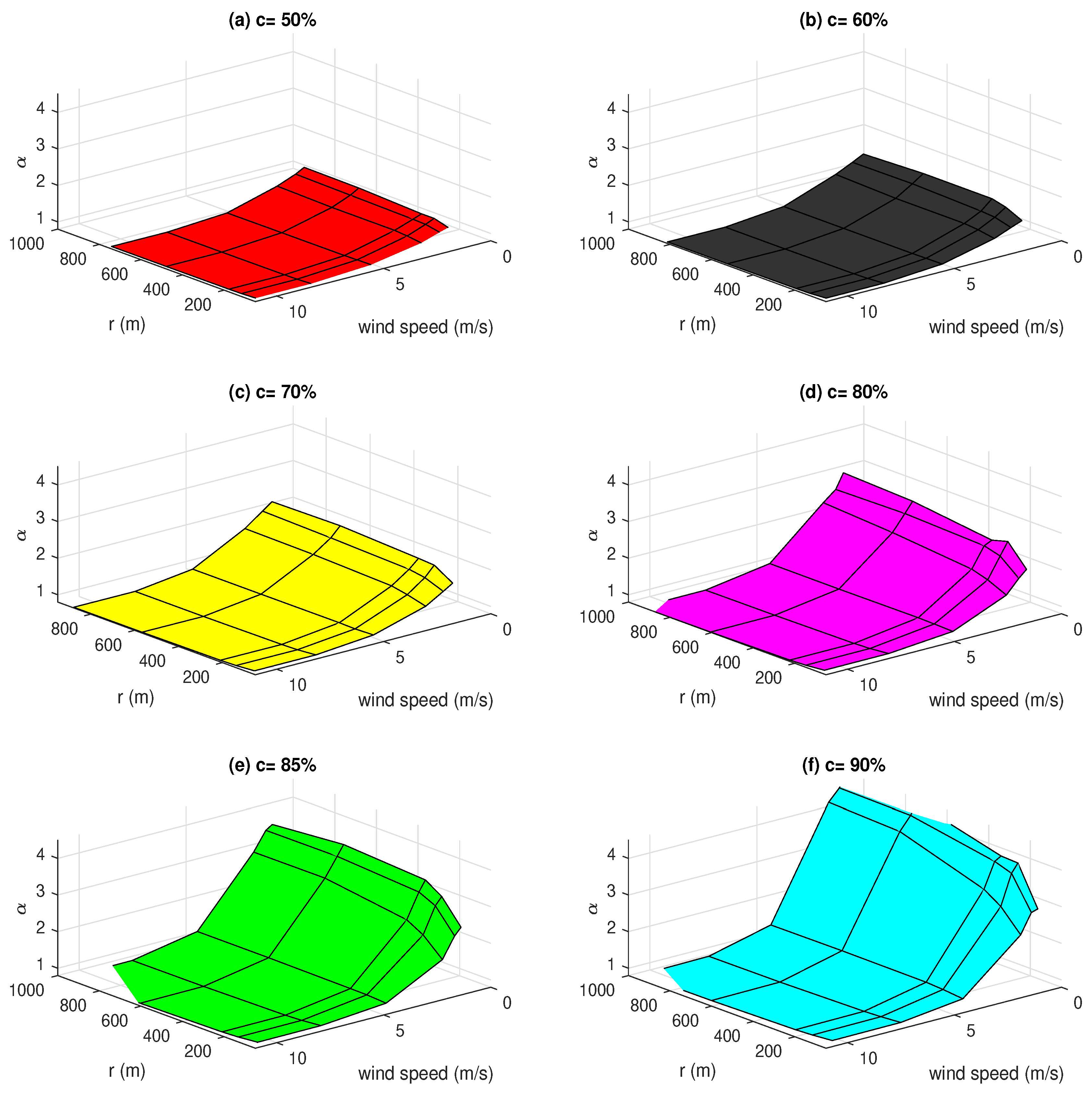
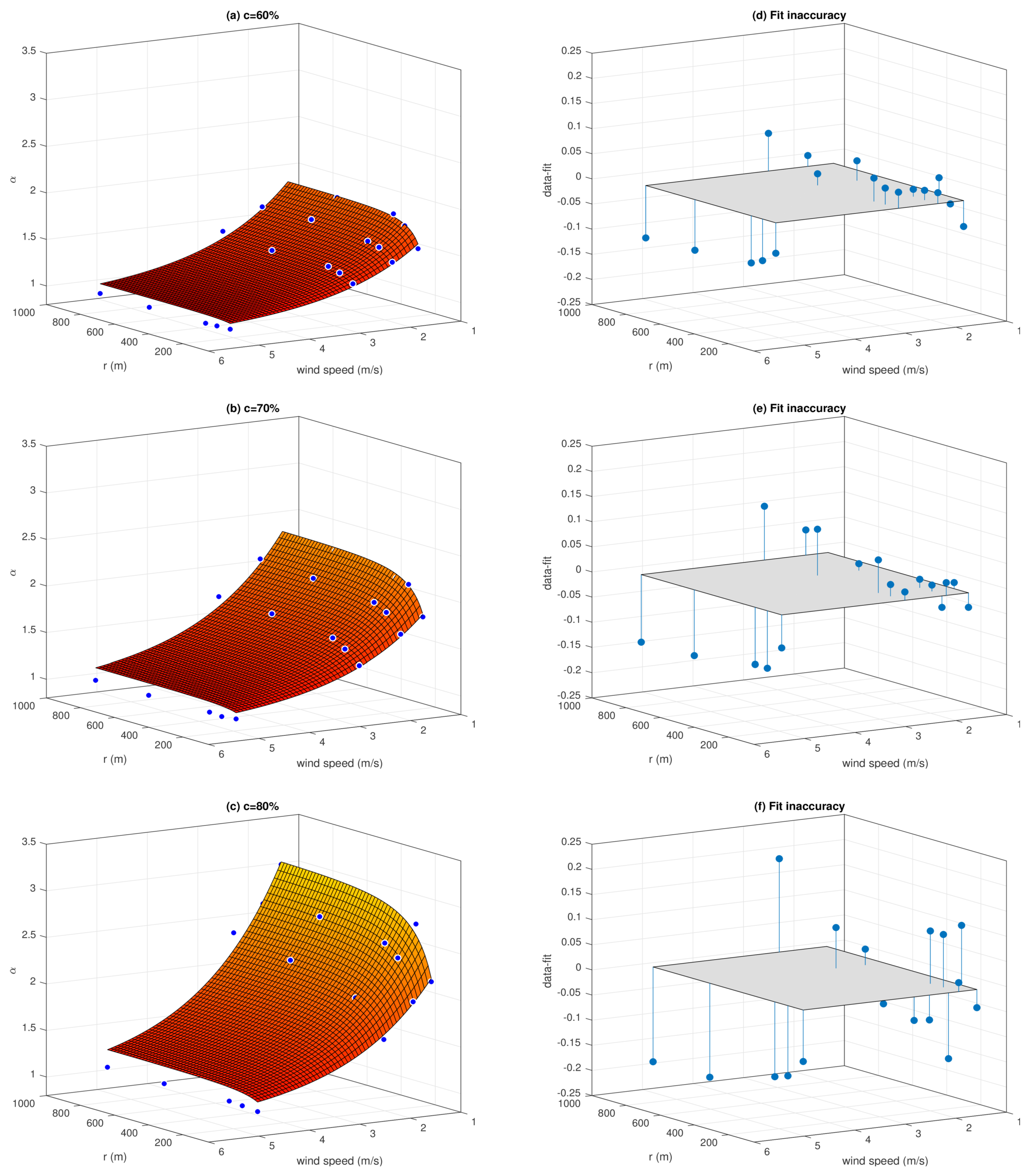
3.2. Correction Coefficient for Surface Moisture Flux

In the preceding study of Wenta and Herman [17] it was found that the basic variables (e.g., temperature, specific humidity) describing the state of the ABL over sea ice are significantly spatially correlated due to the specific three-dimensional structure of convection. The surface turbulent heat fluxes are nonlinear functions of those variables. Assuming that our model domain represents a single grid cell of an NWP model, the characteristic scales of aforementioned convective structures are smaller than the mesh size. Therefore, when only grid-scale atmospheric properties are available and local covariance between them is unknown, assessing the strength of turbulent heat exchange is biased and problematic. In this section, we develop a correction coefficient $\alpha$, described in Section 2.3, for the calculation of moisture heat flux in the situations where the sub-grid variability of surface fluxes is influenced by the FSD.

As described earlier, cold atmospheric conditions present at the beginning of our simulations (251 K) and relatively warm water surface between the sea ice floes (271.4 K) generate rapid and substantial moisture exchange. Water vapor plumes develop over the areas of open water where the updraft air motions are strongest, and the local surface turbulent moisture heat flux reaches maximum. In general, relatively large values of STHF are found over open water areas, with maximum in the regions of convective updrafts, while over sea ice the STHF is close to zero or marginally negative. Therefore, as the FSD determines the spatial arrangement and intensity of convective updrafts, it also controls the distribution and intensity of STHF.

As described in Section 2.3, the correction coefficient $\alpha$ is a function of the mean wind speed $U_m$, median floe size r, and sea ice concentration c. The set of those three variables defines each WRF simulation, for which a single, time-mean value of $\alpha$ is obtained. At first, the coefficients are examined for every sea ice concentration used in the simulations (Figure 5). It is evident that the higher the sea ice concentration, the higher is the value of $\alpha$. Hence, the lower is the sea ice concentration, the less erroneous is the averaging of surface and atmospheric properties, whereas, when sea ice dominates in the model domain ($c\ge 80\%$) the aggregation process will result in disregarding effects of small convective updrafts between each individual floe. Furthermore, for wind speeds higher than ∼6 m/s the value of $\alpha$ approaches one, indicating that the influence of floe size becomes irrelevant. It is a consequence of more intensive mixing of the air in the ABL and homogenization of its properties over sea ice floes and water. As far as the role of FSD is concerned, the values of $\alpha$ are slightly higher for smaller sea ice floes than for bigger floes. It seems reasonable to assume that with decreasing size of the floes, $\alpha \to 1$, i.e., the conditions approach those with a uniform, constant sea ice concentration everywhere in the model domain.

In general, as can be seen in Figure 5, while the significance of mean wind speed and floe-size changes with changing sea ice concentrations, the overall shape of the $\alpha (U_m,r)$ relationship remains similar. The higher the sea ice concentration, the lower the mean wind speed and the bigger sea ice floes are present in the model domain, the higher is the value of $\alpha$. Therefore, we presume that $\alpha$ can be expressed by a single equation which includes the influence of wind speed, sea ice concentration and floe size.

After a comprehensive analysis, the objective of which was to propose a single formula suitable for a wide range of conditions, the following function has been selected:

$$\alpha =1+atanh(b\sqrt{r})e^{d{U}_m},$$

(9)

where the coefficients a and b depend on ice concentration and d is a constant:

$$a=9.1c^{2.11},b=0.152+0.006(1-e^{2.8c}),d=-0.6.$$

(10)

For a given ice concentration, it exhibits the desired behavior in the limiting cases of large wind speeds ($\alpha \to 1$ for $U_m\to \infty$), very small ice floes ($\alpha \to 1$ for $r\to 0$) and large floes ($\alpha$ becomes floe-size independent for $r\to \infty$).

Considering that the accuracy of each particular fit and the general shape of the fitted surface are similar for all sea ice concentrations, only three examples are presented in Figure 6. Elementary statistics, i.e., the correlation coefficient (CC) and the root mean squared error (RMSE) describing the goodness of fit are shown in

Table 1. Statistics describing the goodness of fit of Equation (9).

c	RMSE	CC
50%	0.29	0.98
60%	0.05	0.99
70%	0.11	0.99
80%	0.07	0.99
85%	0.17	0.99
90%	0.18	0.99

. In general, very high values of CC are obtained for every ice concentration, while the values of RMSE change slightly with c. The highest RMSE is found for $c=50\%$, which corresponds to generally small influence of floe size on the $\alpha$ coefficient. Taking into account the nonlinear relationship between the analyzed variables, the obtained high values of CC must be treated with caution. In general, while a high CC is a necessary condition for a fit to be regarded as satisfactory, it is not a sufficient measure of the goodness of fit and has to be completed by other statistics and the analysis of residuals [45]. As can be seen in Figure 6, the algorithm tends to slightly overestimate the values of $\alpha$ in the range of higher wind speeds (where those values are close to 1), but in general, the random scatter of differences between the fitted and the original values of $\alpha$, and small values of those differences, indicate that the proposed approximation produces reasonable results over the range of wind and sea ice conditions considered. Given the modeling results, the derived equation can be used to compute the coefficient $\alpha$ and to correct the value of the moisture flux derived from the area-averaged surface and atmospheric properties.

4. Discussion

We have shown in this study that the floe-size distribution plays an important role in sea ice–atmosphere interactions in the polar regions. It controls the spatial arrangement of sea ice and open water areas together with the associated convective structures in the ABL. Convective updrafts occur in every one of our simulations, but their intensity differs with varying FSD due to the changing extent and strength of breeze-like circulation. Our results are similar to the study of Esau [22], who showed that secondary circulations like the ones found in our modeling results might be of large importance in the studies of ABL convection. Furthermore, his results do not entirely agree with the assumption that narrow leads produce more intensive fluxes, claiming that the associated processes are much more complicated and still not fully understood. Furthermore, in their study of atmospheric response to various configurations of polynya, Dare and Atkinson [16] point out that the spatial arrangement of polynyas influences the magnitude and spatial distribution of vertical heat transfer in the atmosphere. The spaces between the floes in our results vary from a few meters to several kilometers, but in order to fully understand the atmospheric processes above them we also have to examine the size of adjacent floes and the extent of the associated breeze-like circulations. Therefore, our results agree with the suggestions of [16,22] that, when studying the atmospheric response to sea ice fragmentation, the effects related to the spatial arrangement and size distribution of leads and floes must be considered.

Large local differences in atmospheric properties over ice with different floe-size distributions, associated with convective structures, are disregarded when the atmospheric quantities like air temperature or humidity are averaged over the whole model domain. Furthermore, Wenta and Herman [17] pointed out that even when all other initial conditions remain identical, different results of area-averaged fluxes are obtained for the same ice concentration, but different FSDs—which further indicates that the lack of FSD information in NWP models may be at least partially responsible for the observed errors in the simulations over polar regions [1,2]. Based on our WRF modeling results, we propose a simple correction method in the form of an $\alpha$ coefficient that might be used in computation of the surface moisture flux from area-averaged surface and atmospheric variables. The value of $\alpha$ depends on the mean wind speed, sea ice concentration and the median floe radius from particular FSD. In view of the fact that models do not include FSD or the size of the floes in particular grid cell and that presented results have not been validated with observational data, the proposed coefficient is not yet applicable for the GCMs. However, it indicates that the processes associated with the FSD and atmosphere interactions can be parametrized in a simple, computationally efficient way. With the development of models like Horvat et al. [36], Roach et al. [38] such straightforward solution, which includes the effects of different spatial arrangement and sizes of the floes, may soon become applicable in GCMs.

In general, the present research complements that of Wenta and Herman [17] and provides an explanation of the effects described there. The differences in area-averaged values of turbulent fluxes, water vapor and liquid water content in simulations with different FSDs found in [17] are explained based on the fact that FSD determines the spatial arrangement and intensity convection, which in turn controls the exchange of heat and moisture. Furthermore, the problem of high variability of local atmospheric conditions due to surface heterogeneity is addressed further and the first attempt to develop a coefficient integrating the effects of FSD into the calculation of surface moisture flux is made. The development of parametrization in the form of coefficient $\alpha$ will be continued in the subsequent research based on field observations and modeling with the full version of WRF model. Nonetheless, the results presented here provide new insights into the complex influence of sea ice fragmentation on the atmospheric boundary layer. In our opinion, the effects of FSD on the ABL can and should be included in the regional and global weather and climate models, as it is very likely that they are responsible for some of the known inaccuracies present in models results. Furthermore, it is expected that due to the ongoing warming of the Arctic region, sea ice fragmentation in winter is going to become more prevalent, thus further increasing the importance of properly taking into account sea ice heterogeneity in numerical models. Undoubtedly, more field campaigns are needed to improve our understanding of specific processes in situations with various sizes, shapes and orientations of ice floes and open water areas.

It must be noted that present study is based on an idealized model setup and that the results have not been validated with observations. It is a serious limitation. However, as already discussed in the previous paper [17], the crucial aspects of the simulated processes in our results are realistic and have been observed in other modeling and observational studies in the polar regions (e.g., [8,13,46,47]). Furthermore, the described analysis provides an invaluable support in planning of our further research which will include observations and modeling of atmospheric response to sea ice fragmentation in the Bay of Bothnia (Baltic Sea). The aim in this follow-up study is to confirm, based on the field data that FSD does affect the ABL properties and circulation, and to determine to which degree it controls the spatial arrangement and intensity of convective structures within the ABL.

Finally, it is worth noticing that the correction method presented here, based on a coefficient defined as the ratio of the “true” and biased value of the moisture flux, is not applicable to the second component of the total turbulent heat flux, namely the sensible heat flux. Whereas the values of the latent heat flux are always positive (with very few exceptions of extremely small negative values), the sensible heat flux can be both positive and negative, and our previous results [17] showed that different estimation methods—analogous to Equations (5), (6) and (9)—might produce results with a different sign, making a correction based on their ratio meaningless. Thus, a different approach will be necessary for an analogous parametrization of the sensible heat flux.

References

1. Vihma, T.; Screen, J.; Tjernström, M.; Newton, B.; Zhang, X.; Popova, V.; Deser, C.; Holland, M.; Prowse, T. The atmospheric role in the Arctic water cycle: A review on processes, past and future changes, and their impacts. J. Geophys. Res. Biogeosci. 2016, 121, 586–620. [Google Scholar] [CrossRef] [Green Version]
2. Proshutinsky, A.; Steele, M.; Timmermans, M. Forum for Arctic Modeling and Observational Synthesis (FAMOS): Past, current, and future activities. J. Geophys. Res. Oceans 2016, 121, 3803–3819. [Google Scholar] [CrossRef] [Green Version]
3. Glendening, J.; Burk, S. Turbulent transport from an arctic lead: A large-eddy simulation. Bound.-Layer Meteorol. 1992, 59, 315–339. [Google Scholar] [CrossRef]
4. Mauritsen, T.; Svensson, G.; Grisogono, B. Wave flow simulations over Arctic leads. Bound.-Layer Meteorol. 2005, 117, 259–273. [Google Scholar] [CrossRef]
5. Lüpkes, C.; Gryanik, V.; Witha, B.; Gryschka, M.; Raasch, S.; Gollnik, T. Modeling convection over arctic leads with LES and a non-eddy-resolving microscale model. J. Geophys. Res. 2008, 113. [Google Scholar] [CrossRef] [Green Version]
6. Zulauf, M.; Krueger, S. Two-dimensional numerical simulations of Arctic leads: Plume penetration height. J. Geophys. Res. 2003, 108, 8050. [Google Scholar] [CrossRef]
7. Gultepe, I.; Isaac, G.; Williams, A.; Marcotte, D.; Strawbridge, K. Turbulent heat fluxes over leads and polynyas, and their effects on arctic clouds during FIRE.ACE: Aircraft observations for April 1998. Atmos.-Ocean 2003, 41, 15–34. [Google Scholar] [CrossRef]
8. Tetzlaff, A.; Lüpkes, C.; Hartmann, J. Aircraft-based observations of atmospheric boundary-layer modification over Arctic leads. Q. J. R. Meteorol. Soc. 2015, 141, 2839–2856. [Google Scholar] [CrossRef]
9. Andreas, E.; Miles, W.; Barry, R.; Schnell, R. Lidar-derived particle concentrations in plumes from Arctic leads. Ann. Glaciol. 1990, 14, 9–12. [Google Scholar] [CrossRef]
10. Ruffieux, D.; Persson, O.; Fairall, C.; Wolfe, D. Ice pack and lead surface energy budgets during LEADEX 1992. J. Geophys. Res. Oceans. 1995, 100, 4593–4612. [Google Scholar] [CrossRef]
11. Alam, A.; Curry, J. Lead-induced atmospheric circulations. J. Geophys. Res. 1995, 100, 4643–4651. [Google Scholar] [CrossRef]
12. Burk, S.; Fett, R.; Englebretson, R. Numerical simulation of cloud plumes emanating from Arctic leads. J. Geophys. Res. Atmos. 1997, 102, 16529–16544. [Google Scholar] [CrossRef]
13. Marcq, S.; Weiss, J. Influence of leads widths distribution on turbulent heat transfer. Cryosphere 2012, 6, 143–156. [Google Scholar] [CrossRef]
14. Lüpkes, C.; Vihma, T.; Birnbaum, G.; Dierer, S.; Garbrecht, T.; Gryanik, V.; Gryschka, M.; Hartmann, J.; Heinemann, G.; Kaleschke, L.; et al. Mesoscale modelling of the Arctic atmospheric boundary layer and its interaction with sea ice. In The ACSYS Decade and Beyond; Atmospheric and Oceanographic Sciences Library 43; Springer: Dordrecht, The Netherlands, 2012; pp. 279–324. [Google Scholar]
15. Qu, M.; Pang, X.; Zhao, X.; Zhang, J.; Ji, Q.; Fan, P. Estimation of turbulent heat flux over leads using satellite thermal images. Cryosphere 2019, 13, 1565–1582. [Google Scholar] [CrossRef] [Green Version]
16. Dare, R.; Atkinson, W. Atmospheric Response To Spatial Variations In Concentration And Size Of Polynyas In The Southern Ocean Sea-Ice Zone. Bound.-Layer Meteorol. 2000, 94, 65–88. [Google Scholar] [CrossRef]
17. Wenta, M.; Herman, A. The influence of the spatial distribution of leads and ice floes on the atmospheric boundary layer over fragmented sea ice. Ann. Glaciol. 2018, 59, 213–230. [Google Scholar] [CrossRef] [Green Version]
18. Batrak, J.; Müller, M. Atmospheric Response to Kilometer-Scale Changes in Sea Ice Concentration Within the Marginal Ice Zone. Geophys. Res. Lett. 2018, 45, 6702–6709. [Google Scholar] [CrossRef]
19. Saunders, P. Sea smoke and steam fog. Q. J. R. Meteorol. Soc. 1964, 90, 156–165. [Google Scholar] [CrossRef]
20. Walter, B.; Overland, J. Observations of Longitudinal Rolls in a Near Neutral Atmosphere. Mon. Weather Rev. 1984, 112, 200–208. [Google Scholar] [CrossRef] [Green Version]
21. Fett, R.; Burk, S.; Thompson, W.; Kozo, T. Environmental Phenomena of the Beaufort Sea Observed during the Leads Experiment. Bull. Am. Meteorol. Soc. 1994, 75, 2131–2146. [Google Scholar] [CrossRef]
22. Esau, I. Amplification of turbulent exchange over wide Arctic leads:Large-eddy simulation study. J. Geophys. Res. Atmos. 2007, 112. [Google Scholar] [CrossRef]
23. Rockel, B.; Will, A.; Hense, A. The regional climate model COSMO-CLM (CCLM). Meteorol. Z. 2008, 17, 347–348. [Google Scholar] [CrossRef]
24. Vihma, T. Subgrid parameterization of surface heat and momentum fluxes over polar oceans. J. Geophys. Res. Oceans 1995, 100, 22625–22646. [Google Scholar] [CrossRef] [Green Version]
25. Arola, A. Parameterization of Turbulent and Mesoscale Fluxes for Heterogeneous Surfaces. J. Atmos. Sci. 1999, 56, 584–598. [Google Scholar] [CrossRef]
26. Heinemann, G.; Kerschgens, M. Comparison of methods for area-averaging surface energy fluxes over heterogeneous land surfaces using high-resolution non-hydrostatic simulations. Int. J. Climatol. 2005, 25, 379–403. [Google Scholar] [CrossRef]
27. Avissar, R.; Pielke, R. A Parameterization of Heterogeneous Land Surfaces for Atmospheric Numerical Models and Its Impact on Regional Meteorology. Mon. Weather Rev. 1989, 117, 2113–2136. [Google Scholar] [CrossRef] [Green Version]
28. Claussen, M. Area-averaging of surface fluxes in a neutrally stratified, horizontally inhomogeneous atmospheric boundary layer. Atmos. Environ. Part A Gen. Top. 1990, 4, 1349–1360. [Google Scholar] [CrossRef]
29. de Vrese, P.; Schulz, J.; Hagemann, S. On the Representation of Heterogeneity in Land-Surface–Atmosphere Coupling. Bound.-Layer Meteorol. 2016, 160, 157–183. [Google Scholar] [CrossRef]
30. Frech, M.; Jochum, A. The Evaluation of Flux Aggregation Methods using Aircraft Measurements in the Surface Layer. Agric. For. Meteorol. 1999, 98–99, 121–143. [Google Scholar] [CrossRef]
31. Kwok, R. Arctic sea ice thickness, volume, and multiyear ice coverage: Losses and coupled variability (1958–2018). Environ. Res. Lett 2018, 13, 105005. [Google Scholar] [CrossRef]
32. Rampal, P.; Weiss, J.; Marsan, D. Positive trend in the mean speed and deformation rate of Arctic sea ice, 1979–2007. J. Geophys. Res. Oceans 2009, 114. [Google Scholar] [CrossRef]
33. Rothrock, D.; Thorndike, A. Measuring the sea ice floe size distribution. J. Geophys. Res. Oceans 1984, 89, 6477–6486. [Google Scholar] [CrossRef]
34. Steele, M. Sea ice melting and floe geometry in a simple ice-ocean model. J. Geophys. Res. Oceans 1992, 97, 17729–17738. [Google Scholar] [CrossRef]
35. Zhang, J.; Schweiger, A.; Steele, M.; Stern, H. Sea ice floe size distribution in the marginal ice zone: Theory and numerical experiments. J. Geophys. Res. Oceans 2015, 120, 3484–3498. [Google Scholar] [CrossRef]
36. Horvat, C.; Tziperman, E.; Campin, J. Interaction of sea ice floe size, ocean eddies, and sea ice melting. Geophys. Res. Lett. 2016, 43, 8083–8090. [Google Scholar] [CrossRef] [Green Version]
37. Horvat, C.; Tziperman, E. A prognostic model of the sea-ice floe size and thickness distribution. Cryosphere 2015, 9, 2119–2134. [Google Scholar] [CrossRef] [Green Version]
38. Roach, L.; Horvat, C.; Dean, S.; Bitz, C. An Emergent Sea Ice Floe Size Distribution in a Global Coupled Ocean-Sea Ice Model. J. Geophys. Res. Oceans 2018, 123, 4322–4337. [Google Scholar] [CrossRef]
39. Herman, A. Discrete-Element bonded-particle Sea Ice model DESIgn, version 1.3a—Model description and implementation. Geosci. Model Dev. Discuss. 2016, 9, 1219–1241. [Google Scholar] [CrossRef]
40. Uttal, T.; Curry, J.; Mcphee, M.; Perovich, D.; Moritz, R.; Maslanik, J.; Guest, P.; Stern, H.; Moore, J.; Turenne, R.; et al. Surface Heat Budget of the Arctic Ocean. Bull. Am. Meteorol. Soc. 2002, 83, 255–275. [Google Scholar] [CrossRef] [Green Version]
41. Janjić, Z. Nonsingular Implementation of the Mellor-Yamada Level 2.5 Scheme in the NCEP Mesoscale Model; Office Note #437; National Centers for Environmental Prediction Office: College Park, MD, USA, 2001.
42. Janić, Z. The Step-Mountain Eta Coordinate Model: Further Developments of the Convection, Viscous Sublayer, and Turbulence Closure Schemes. Mon. Weather Rev. 1994, 122, 927–945. [Google Scholar] [CrossRef] [Green Version]
43. Monin, A.; Obukhov, A. Basic laws of turbulent mixing in the surface layer of the atmosphere. Contrib. Geophys. Inst. Acad. Sci. USRR 1954, 151, 163–187. [Google Scholar]
44. Young, G.; Kristovich, D.; Hjelmfelt, M.; Foster, R. Rolls, Streets, Waves, and More. Bull. Am. Meteorol. Soc. 2002, 83, 997–1002. [Google Scholar] [CrossRef]
45. Canepa, E.; Irwin, J. Chapter 17: Evaluation Of Air Pollution Models. In Air Quality Modeling—Theories, Methodologies, Computational Techniques, and Available Data Bases and Software, V.II – Advanced Topics; The EnvironComp Institute and Air and Waste Management Association: Pittsburgh, PA, USA, 2005; pp. 503–556. [Google Scholar]
46. Zulauf, M.; Krueger, S. Two-dimensional cloud-resolving modeling of the atmospheric effects of Arctic leads based upon midwinter conditions at the Surface Heat Budget of the Arctic Ocean ice camp. J. Geophys. Res. Atmos. 2003, 108. [Google Scholar] [CrossRef]
47. Esau, I.; Sorokina, S. Climatology of Arctic Planetary Boundary Layer. In Atmospheric Turbulence, Meteorological Modeling and Aerodynamics; Langand, P.R., Lombarg, F.S., Eds.; Nova Science Publishers: Hauppauge, NY, USA, 2010; pp. 3–58. [Google Scholar]
Figure 1. An example gray scale image of upward air motion areas within the model area (a) and a corresponding output from Pixie program where the upward air motion areas are marked in black (b).
Atmosphere 10 00654 g001
Figure 2. Wind speed (colors) and wind vectors (arrows) for simulations with c = 70 % , N f = 500 , with weak wind conditions (profile No. 1; a) and stronger wind conditions (profile No. 3; b).
Atmosphere 10 00654 g002
Figure 3. Simulation with weak wind condition (zero initial wind), c = 80 % and N f = 100 , crosswise transect of: vertical velocity component of the air motion (m/s; a), water vapor mixing ratio (kg/kg; b), and atmospheric pressure (hPa; c).
Atmosphere 10 00654 g003
Figure 4. Time-mean total area of convective updrafts (km 2 ; a), time-mean height reached by a convective plume (m; b), total liquid water content (kg/kg; c) and area–averaged sensible heat flux (W/m 2 , d) in function of the number of floes N f , in simulations with c = 90 % , weak wind conditions (ambient wind speed 2 m/s).
Atmosphere 10 00654 g004
Figure 5. Values of the α coefficient for every WRF model simulation with different ambient wind speed U m and median floe size r, plotted for all sea ice concentrations considered in the analysis (af).
Atmosphere 10 00654 g005
Figure 6. Left (ac): values of α computed from Equation (9) (plotted surfaces) and obtained from WRF simulations (dots) for c = 60 % (a), 70% (b) and 80% (c). Right (df): the accuracy of each fit represented by the difference between the original and fitted values.
Atmosphere 10 00654 g006