Article

Climate Extremes over the Arabian Peninsula Using RegCM4 for Present Conditions Forced by Several CMIP5 Models

by
Mansour Almazroui
Center of Excellence for Climate Change Research/Department of Meteorology, King Abdulaziz University, Jeddah 21589, Saudi Arabia
Atmosphere 2019, 10(11), 675; https://doi.org/10.3390/atmos10110675
Submission received: 24 September 2019 / Revised: 18 October 2019 / Accepted: 25 October 2019 / Published: 2 November 2019

Abstract

:
This paper investigates the temperature and precipitation extremes over the Arabian Peninsula using data from the regional climate model RegCM4 forced by three Coupled Model Intercomparison Project Phase 5 (CMIP5) models and ERA–Interim reanalysis data. Indices of extremes are calculated using daily temperature and precipitation data at 27 meteorological stations located across Saudi Arabia in line with the suggested procedure from the Expert Team on Climate Change Detection and Indices (ETCCDI) for the present climate (1986–2005) using 1981–2000 as the reference period. The results show that RegCM4 accurately captures the main features of temperature extremes found in surface observations. The results also show that RegCM4 with the CLM land–surface scheme performs better in the simulation of precipitation and minimum temperature, while the BATS scheme is better than CLM in simulating maximum temperature. Among the three CMIP5 models, the two best performing models are found to accurately reproduce the observations in calculating the extreme indices, while the other is not so successful. The reason for the good performance by these two models is that they successfully capture the circulation patterns and the humidity fields, which in turn influence the temperature and precipitation patterns that determine the extremes over the study region.

1. Introduction

In the past two decades, the evidence of climate change has become more obvious and it is widely accepted that, besides natural variability, human activities are significantly enhancing the change in climate [1]. The Intergovernmental Panel on Climate Change (IPCC) fifth assessment report (AR5) highlights the increasing global mean temperature and the fact that it will continue to increase throughout the 21st century [2]. According to the IPCC fourth assessment report (AR4), for the period 1956–2005, the global mean surface temperature (both land and ocean) increased by 0.13 °C/decade [3] which was updated in AR5 to 0.12 °C/decade for the period 1951–2012 [2]. The observations show that surface temperature over the Arabian Peninsula, in particular over Saudi Arabia (covering 80% of the peninsula), increased at a rate of 0.60 °C/decade for the last three decades [4]. This large rate of increase in surface temperature over the Peninsula causes many temperature extremes in the region and indicates the need for a disaster management program [5]. In a recent study Almazroui et al. [6] presented evidence that during the 21st century, temperature over the Peninsula will warm at a faster rate than over the larger COordinated Regional climate Downscaling Experiment (CORDEX) Middle-East and North Africa (MENA) domain. In addition to this rise in temperature, changes in precipitation were also observed over the Peninsula. Observations show that in recent decades, precipitation over Saudi Arabia has followed a decreasing trend (a drop of 47.8 mm/decade for the period 1978–2009 [4]), although the number of heavy precipitation events has increased in the last decade. Recently, Atif et al. [7] assessed extreme precipitation events over the Peninsula based on observations from 1984–2016. They reported a high number of extreme precipitation events over northeastern, central and southwestern coastal parts of Saudi Arabia. Saeed and Almazroui [8] reported on the relationship between largescale circulation and winter precipitation over the Arabian Peninsula using observations for the period 1948–2012. Based on observations for the period 1970–1099, extreme precipitation contributes about 40% (70%) of the total amount of rainfall during the wet (dry) season in the Arabian Peninsula (Almazroui and Saeed 2020 [9]). These trends, the large rate of increase in temperature, the decrease in precipitation and the increase in heavy precipitation events, all amount to a timely call for an in–depth study of climate extremes in the region.
Predicting climate extremes such as temperature and precipitation is important for assessing vulnerability on the local to regional scale. Moreover, climate extremes can have devastating socioeconomic and environmental impacts on a region [10]. Climate extremes have major impacts on sectors such as water resources, agriculture, food security, and energy production [11]. Climate extremes are also important in this era of climate change because a changing climate leads to changes in the frequency and intensity as well as the duration of extreme climate events [2]. In the AR4, reference is made to the fact that both minimum and maximum temperatures have shifted to higher values [3]. This shift is bringing about a warmer environment in which cold extremes are warming faster than the warm extremes.
In general, temperature and precipitation extremes are calculated from daily data for point locations [12,13,14,15], for a region e.g., [1,16], or for the whole globe e.g., [17,18,19]. Daily data are used in the calculation of many temperature indices such as warm or cold days, and of precipitation indices such as wet or dry spells including heavy precipitation events. In the calculation of these indices of extremes, different thresholds and procedures may apply, depending on the focus of the researcher, which makes it difficult to define an index [20]. To overcome this problem and to focus on relevant climate aspects, a standard procedure to analyze such extremes and to define a number of climate extreme indices was proposed by the Expert Team on Climate Change Detection and Indices (ETCCDI) [20,21]. The ETCCDI–defined extremes indices have been used over the last decade by many researchers [13,14,18,19].
Over the Arabian Peninsula, several research studies on climate extremes using ETCCDI were conducted using surface temperature and precipitation data [13,15]. Some information on climate extremes over the Arabian Peninsula is also available from analysis using IPCC AR4 (CMIP3) and AR5 (CMIP5) multi-models data [18]. However, to the best of our knowledge, details on the analysis of extremes using CMIP5 multi–models downscaled by regional climate model and compared with the observations are not available for the region except for the work of Almazroui [6] who showed that threshold based warm days (Tmax  ≥  50 °C) will increase and cold nights (Tmin  ≤  5°C) will decrease faster over the Arabian Peninsula than over the wider region. Nevertheless, no climate model simulation is free from uncertainty and that in particular, the simulation of precipitation and temperature on a daily scale is a challenging task. Therefore, the comparison of extremes indices calculated from model data with data obtained from surface observations is essential. To this end, the focus of this study is to evaluate how well the regional climate model performs in downscaling CMIP5 data to calculate climate extreme indices by comparing them with the corresponding surface observations over the Arabian Peninsula for the present climate. The comparison will be extended into the projection period in a subsequent document.
The paper is organized as follows: the data and methodology including the regional climate model experimental setup are discussed in Section 2. The results and discussion are given in Section 3 while the conclusions are drawn in Section 4.

2. Data and Methodology

2.1. Data

This study uses daily maximum and minimum temperatures and precipitation data from 27 surface observations stations across Saudi Arabia (see Almazroui et al. [4] for meteorological station names and locations) collected by the General Authority of Meteorology and Environmental Protection (GAMEP) over the period 1978–2016. These data are processed through quality control and corrected by metadata where applicable. In case of missing metadata data from surrounding stations are used to fill the gap. Data from the weather underground database are also checked (Almazroui et al. [4]).
The RegCM4–generated temperature and precipitation climatology for the Arabian Peninsula domain is compared with results obtained from the gridded observational dataset, namely, the updated Climatic Research Unit (CRU) TS3.23 data [22]. The CRU data encompasses surface observations over land throughout the world. However, in some regions, the data collection network is of low density, e.g., the distribution of stations used by CRU over the Sahara Desert is quite sparse (Tsikerdekis et al. [23]).

2.2. Methodology

2.2.1. Regional Climate Model and Experimental Setup

In generating the daily temperature and precipitation data for the calculation of climate extremes indices over the Arabian Peninsula, the output from three CMIP5 models, namely ECHAM6 (Atmospheric Global Climate Model of Max Planck Institute for Meteorology, Germany, resolution: 1.80°×1.80°), GFDL (Geophysical Fluid Dynamics Laboratory, USA, resolution: 2.50° × 2.00°), and HadGEM (UK Met Office Hadley Centre Global Environment Model version 2, resolution: 1.875°×1.25°), are downscaled using REGional Climate Model version 4 (RegCM4.7) for the current climate (1960–2005). The regional climate model data are generated with the input of three CMIP5 multi–model databases used in the preparation of AR5. RegCM4, developed in the Abdus Salam International Centre for Theoretical Physics (ICTP), Trieste, Italy is one of the most widely used regional climate models. Details of the RegCM4 are available in [24]. Among its many physical and dynamical features, RegCM4 has two land surface schemes that are used in this study, namely (i) the Biosphere and Atmosphere Transfer Scheme (BATS version 1e, [25,26]) and (ii) the Community Land Model (CLM version 4.5, [27]). Some land surface types such as ice, glacier, bog/marsh, and irrigated crops are very sensitive to the land surface module used, but in the Arabian Peninsula analysis domain these types are almost entirely absent. In general, BATS is used to describe the role of soil moisture and vegetation in the model. The exchange of momentum, energy, and water vapor across the surface-atmosphere interface are calculated in the BATS module. For details, see Dickinson et al. [26]. The CLM uses a mosaic approach for capturing land surface heterogeneity at each grid in the model. The subgrid tiles approach used in CLM enables it to represent various surface parameters in a more detailed way than in BATS (Steiner et al. [28]). For detail about CLM, see Oleson et al. [27]. The main advantage of CLM is that it has a higher number of soil layers and vegetation fractions than in BATS. Following Fritsch et al. [29], the convective schemes of Grell with Fritsch–Chappell closure (GFC, [30,31]) are used. RegCM4 is forced with ERSST, the Extended Reconstructed Sea Surface Temperature data, obtained from the National Climate Data Centre (NCDC). Following Harris et al. [32], the effective domain used stretches from the Equator to 45 °N, and from 17 °E to 72 °E, covering the Arabian Peninsula and its surroundings. The following RegCM4 experiments were run:
To evaluate the performance of RegCM4 in simulating the climate of the study region, the RegCM4 was forced with widely used ERA–Interim re–analysis (0.75° × 0.75°) gridded 6-hourly data (http://www.ecmwf.int/products/data/archive) using the BATS land–surface scheme for the available period 1979–2015 (with 1979 used as spin–up time).
  • Step (i) was repeated using the CLM land–surface scheme.
  • RegCM4 was forced with GFDL using BATS for the period 1970–2005 (with 1970 used as spin–up time).
  • Step (iii) was repeated using the CLM land–surface scheme.
  • RegCM4 was forced with HadGEM output using BATS for the period 1960–2005 (with 1960 used as spin–up time).
  • Step (v) is repeated using the CLM land–surface scheme.
  • RegCM4 was forced with ECHAM6 output using BATS for the period 1960–2005 (with 1960 used as spin–up time).
  • Step (vii) was repeated using the CLM land–surface scheme.
All RegCM4 runs were performed with 25 km horizontal resolution and 18 vertical levels.

2.2.2. Analysis Procedure

The bias (model minus observation) for temperature (in °C) and precipitation (in percentage) was obtained from the model with respect to the CRU monthly data. Simulated temperature and precipitation daily data were used to calculate climate extremes indices for the study region.
There is a core set of 27 extremes indices recommended by the ETCCDI [18]. The definition of these extremes indices can be seen in the literature [13,14,15,18]. The threshold of each station is different from the threshold of the other stations, as defined in RClimDex, a software package recommended by ETCCDI. All of these 27 indices are first calculated using surface observations from 27 stations located across Saudi Arabia for the period 1978–2016 (Table 1). The description of station characteristics and the methodology of the homogeneity test including data quality control and control for missing data from these stations are available in Donat et al. [13] and Islam et al. [14]. Some indices such as ice days (the number of days when the daily minimum temperature falls below zero) and warm days (the number of days when the daily maximum temperature is above 25 °C) are not useful for this study area because they are not relevant to this sub-tropical semi–arid and arid region. Using ETCCDI, Donat et al. [13] calculated 11 temperature indices for Saudi Arabia, while You et al. [15] calculated 13 with 11 of them in common, using surface observations for the period 1981–2010. Almazroui et al. [33] also calculated 11 temperature indices over South Asia using surface observations for the period 1971–2000 while Alexander et al. [16] analyzed five temperature indices using data from 303 meteorological stations in China for the period 1961–2003. For the sake of brevity, this analysis focused on the calculation of nine climate extremes indices, namely,
  • Warm days (TX90p, a percentile index calculated from daily maximum temperature),
  • Warm nights (TN90p, a percentile index calculated from daily minimum temperature),
  • Cold days (TX10p, a percentile index calculated from daily maximum temperature),
  • Cold nights (TN10p, a percentile index calculated from daily minimum temperatures),
  • Warm spell duration (WSDI, an index is calculated from daily maximum temperatures),
  • Cold spell duration (CSDI, an index calculated from daily minimum temperature),
  • Number of wet days (R1mm, number of wet days is a threshold index calculated from daily precipitation),
  • Consecutive wet days (CWD, a threshold index calculated from daily precipitation),
  • Consecutive dry days (CDD, a threshold index calculated from daily precipitation) from the climate model data for the study region.
The reason for selecting these indices was to see how well the model simulated daily data for the calculation of extremes indices over the study region. Spatial distribution of the above-mentioned extremes indices, obtained from RegCM4 forced by three CMIP5 models with two land–surface schemes, is compared with the spatial distribution obtained from RegCM4 forced with ERA–Int data for the same period 1986–2005. The period 1986–2005 was selected because surface observation data were available for all 27 stations. Another reason for selecting 1986–2005 is that in extremes indices calculation using ETCCDI, a reference period is required, which is taken as 1981–2000. Also, Sillmann et al. [17] used this period, 1981–2000, as a reference period. The extreme indices calculated from model data were extracted at the nearest grid point to the station locations and then compared with those calculated from surface observations. The climate extreme index trends were calculated using linear regression for each index at all 27 locations. The significance of the climate extreme indices trends is obtained using the F–test. Surface observations were used to assess the RegCM4 performance as well as the land–surface process and CMIP5 models. A normal quantile plot was used to see how well the daily data values fit a normal distribution for temperatures (maximum and minimum) and for precipitation, as obtained from CMIP5 models downscaled by RegCM4, from ERA–Int reanalysis, and from surface observations.

3. Results and Discussion

This section describes the extremes indices results obtained from surface observations and model simulations.

3.1. Temperature and Precipitation Simulations

Before proceeding to the calculation of extremes indices using model simulations, the temperature (maximum and minimum) and precipitation climatology was investigated over the study area. Note that the performance of RegCM4 was not evaluated with different CMIP5 forced data because a RegCM4 evaluation has already performed by Almazroui et al. [34].

3.1.1. Temperature Simulation

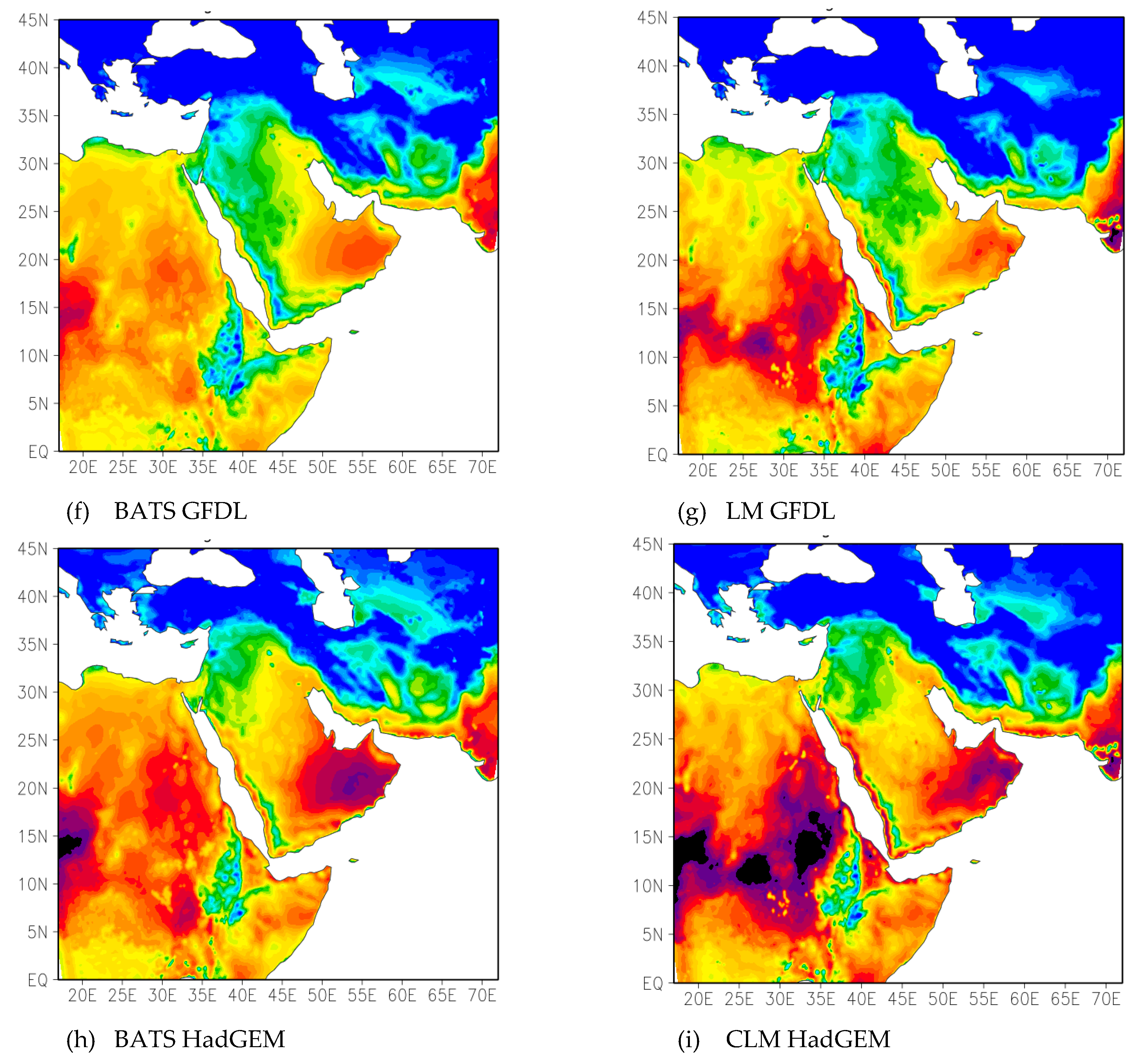
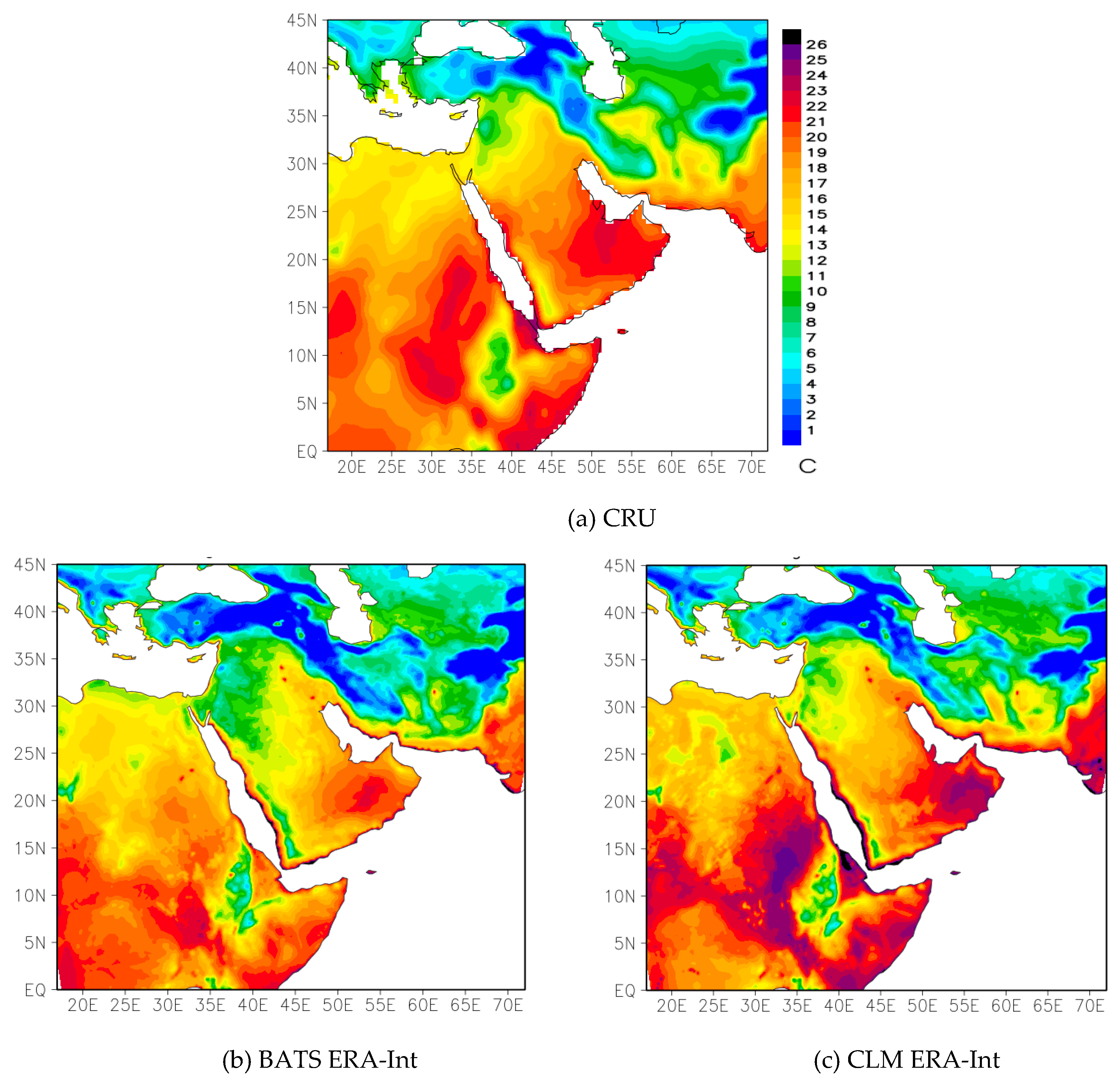
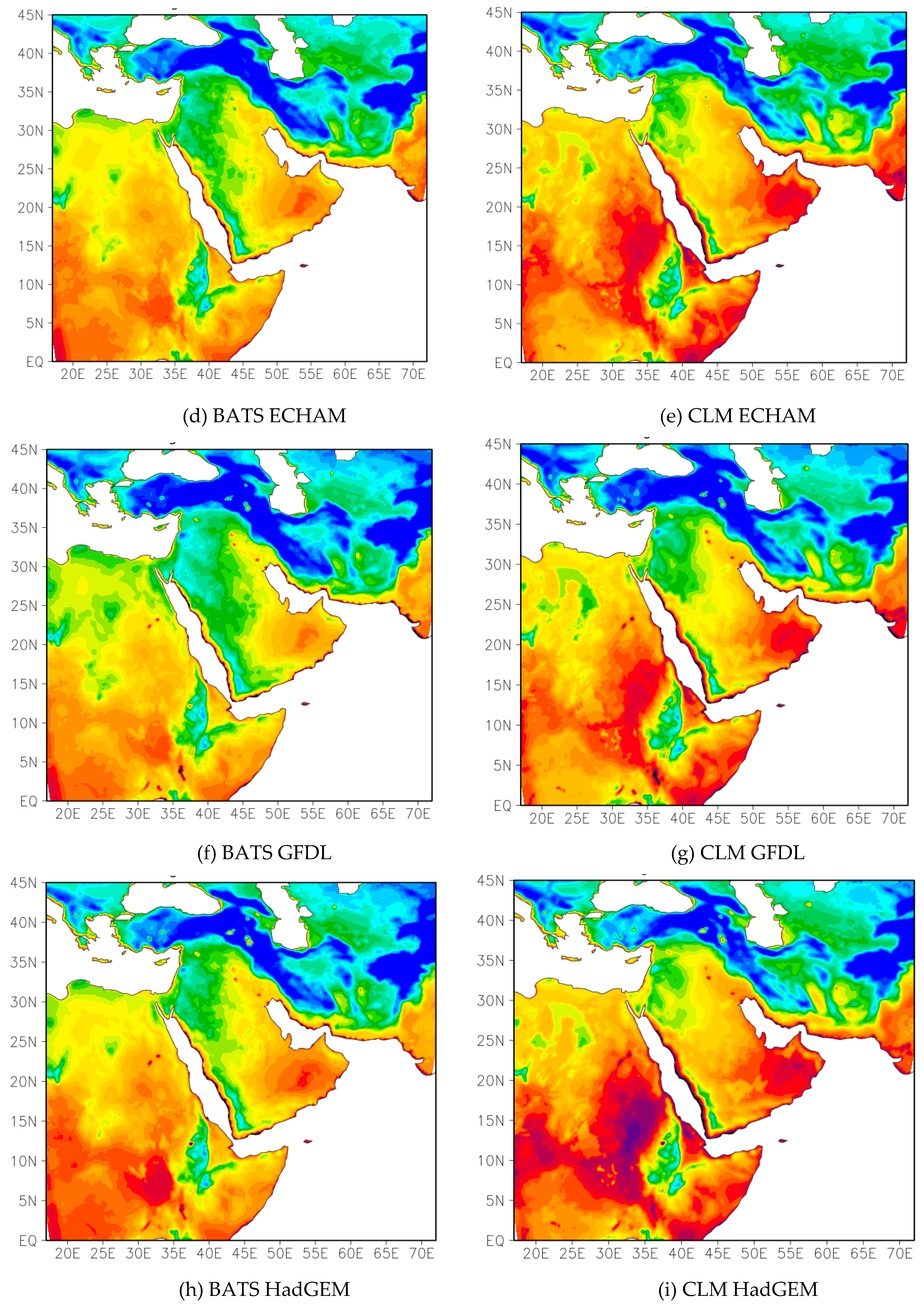
Daily maximum and minimum temperatures are the key parameters in the calculation of temperature extremes. Therefore, the climatology of these parameters from model simulations is displayed, along with CRU data, in Figure 1 and Figure 2. In general, the patterns of simulated maximum and minimum temperatures follow the patterns of the CRU data with some variations such as the highest maximum temperature simulated in the southeast Peninsula in all experiments not appearing in the observations. Very close scrutiny indicates that there is a difference between the observation and simulations, which reflects the limitation of climate models in capturing climatic information at the local level. Simulated temperatures are higher than the observations in the southeast and lower in the northwest parts of the peninsula. This temperature pattern was also reported by Almazroui et al. [35], and Ehsan et al. [36] for the CORDEX-MENA/Arab domain, for the simulation of mean temperature using RegCM4. The maximum temperature is overestimated by the model in most simulations, particularly in the southwestern and coastal areas (Figure 1). However, the bull’s eye–shaped overestimation over Oman in the BATS case is slightly reduced in the CLM simulation. The simulated maximum temperature is overestimated compared to the CRU reanalysis data, by over 5.5 °C in the southeastern and coastal areas of the peninsula (Supplementary 1). For the case of GFDL, a slight underestimation of maximum temperature is observed in the central to western areas. The simulated minimum temperature is overestimated in the southeast and coastal areas of the peninsula, although it is underestimated in the western and northern areas of the peninsula (Figure 2). These over–and underestimations are clearly seen in the bias pattern shown in Supplementary 2, and the underestimation is more prominent in BATS than CLM, reaching a difference of −5.5 °C. In the GFDL case, the underestimation of minimum temperature is observed all over the peninsula. Overall, the patterns of maximum and minimum temperature climatology follow the patterns of the CRU reanalysis data, although magnitudes vary from model to model and between the different land–surface schemes.

3.1.2. Precipitation Simulation

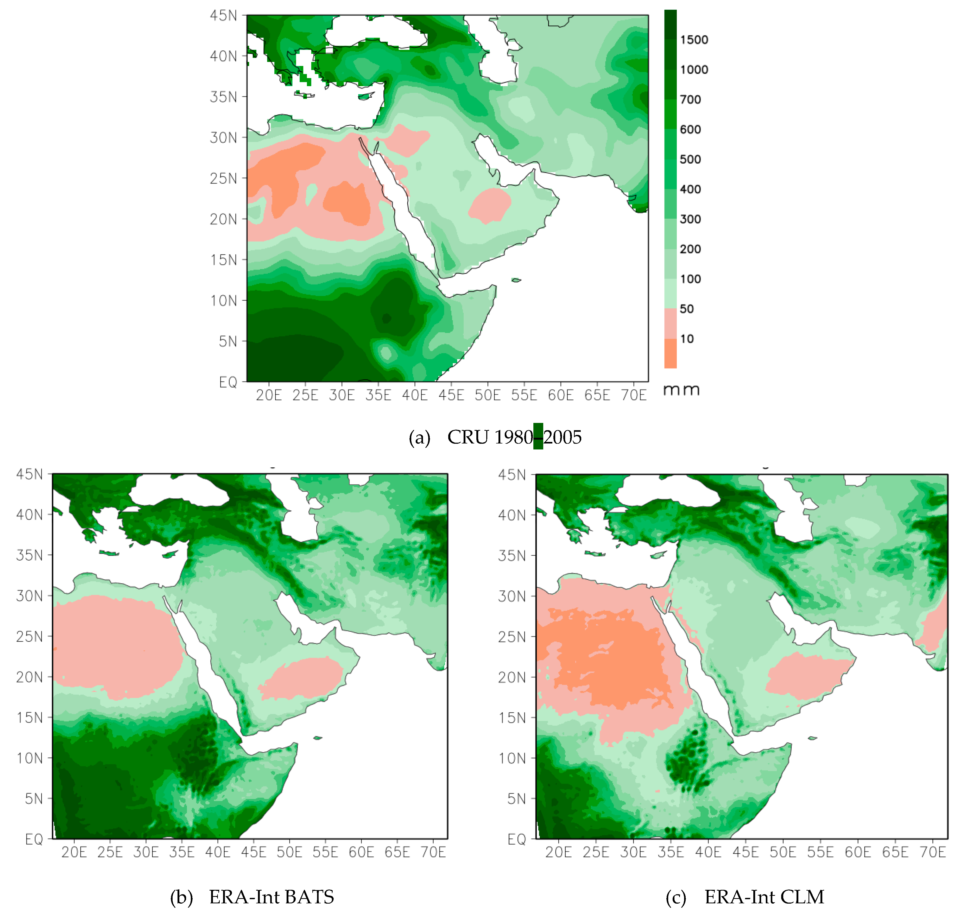
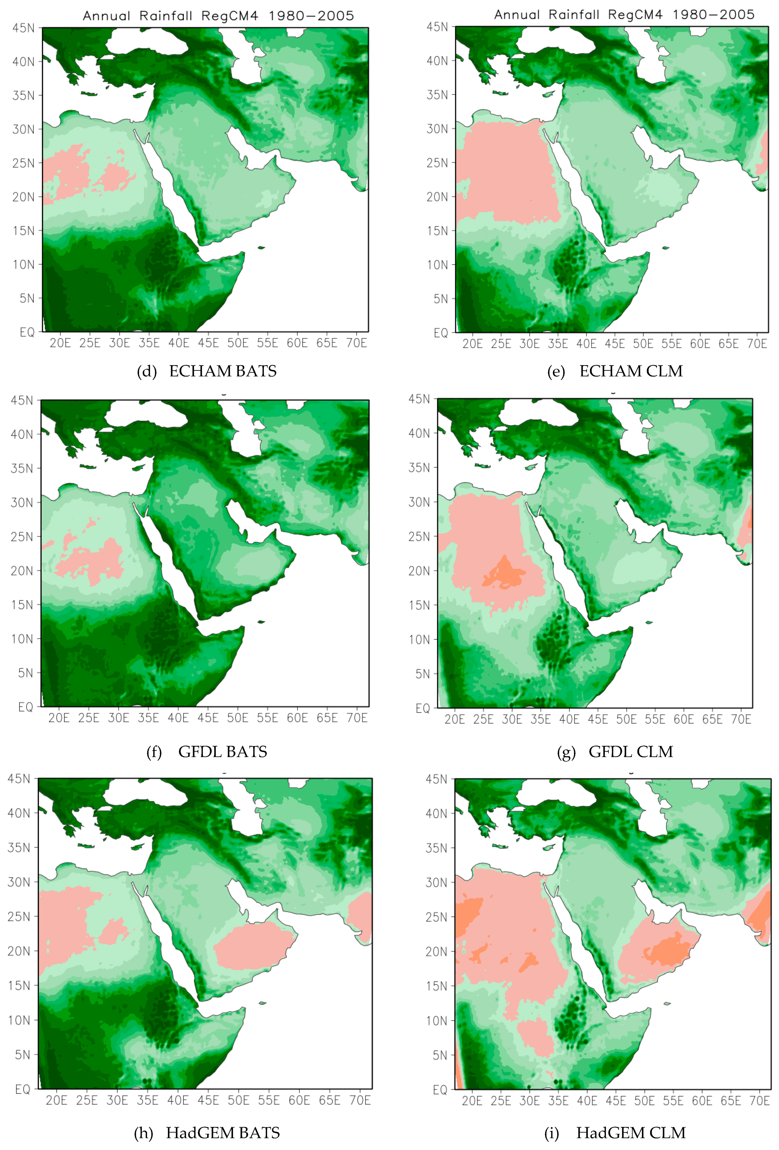
In the calculation of precipitation extremes indices, daily precipitation is the key parameter. The climatology of precipitation from the model and CRU data is shown in Figure 3. The pattern of simulated precipitation closely follows the observed pattern obtained from CRU data, particularly the small amount of rainfall in the southeast and the heavy rainfall in the central to northern areas. These precipitation patterns are similar to the RegCM4 output for the CORDEX–MENA/Arab domain [35]. Comparing the two land–surface schemes, the BATS simulated enhanced precipitation is generally higher than in the simulation using CLM. The rainfall bias clearly shows that the ECHAM and GFDL–forced–simulations overestimate precipitation over the Arabian Peninsula, although the HadGEM and ERA–Int–forced simulations show underestimation in the south and overestimation in the north (Supplementary 3). Again, for precipitation, the patterns of simulated climatology are similar to the observations, although values vary depending on the different model setups, boundary conditions, and land–surface schemes.

3.2. Climate Extremes Indices

3.2.1. Observation-Based Climate Extremes

Daily temperature and precipitation data from 27 surface observational stations across Saudi Arabia are used in the calculation of ETCCDI-defined extremes indices (Table 1). The trend of each index presented on a decadal scale shows that some are increasing while others are decreasing over the entire observational data period 1978–2016. The direction of all of the trends is similar to those found by AlSarmi et al. [11] except for CDD and R95p. The difference in direction for these two indices might be due to the use of a large number of updated station data in the current study. Only four of the trends are significant. It is important to note that the study region warmed because the number of warm days/nights increased significantly while the number of cold nights decreased significantly. Though not statistically significant, the number of wet days and total wet–day precipitation are showing decreasing trends. Since the aim of this paper is to explore the potential to use climate model output in the calculation of climate extremes, some of the simulation–based climate extreme indices are summarized in the next Section.

3.2.2. Simulation-Based Climate Extremes

Using climate model data in the calculation of climate extremes is a challenging task because state-of-the-art climate models are not free from uncertainties, with the simulated daily data, in particular, showing large biases (see Supplementary 1, 2, and 3) and the simulation of more precipitation days than are observed. This section discusses the simulation-based climate extremes and compares them with the same obtained from observations over the same period.

3.2.3. Temperature Extremes

There are 16 temperature extreme indices on the ETCCDI recommended list (from the top in Table 1) of which six are discussed here.
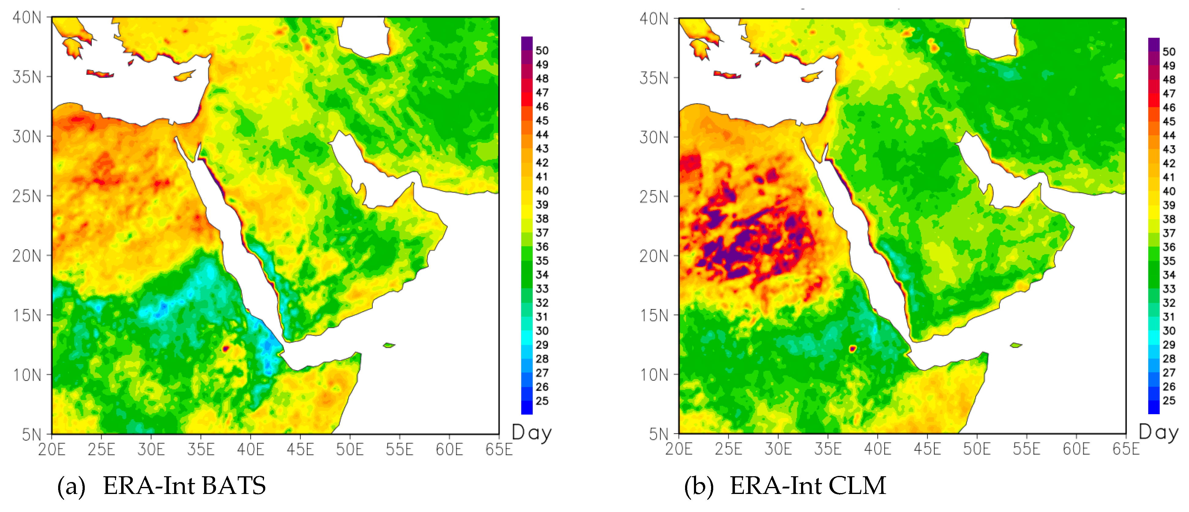
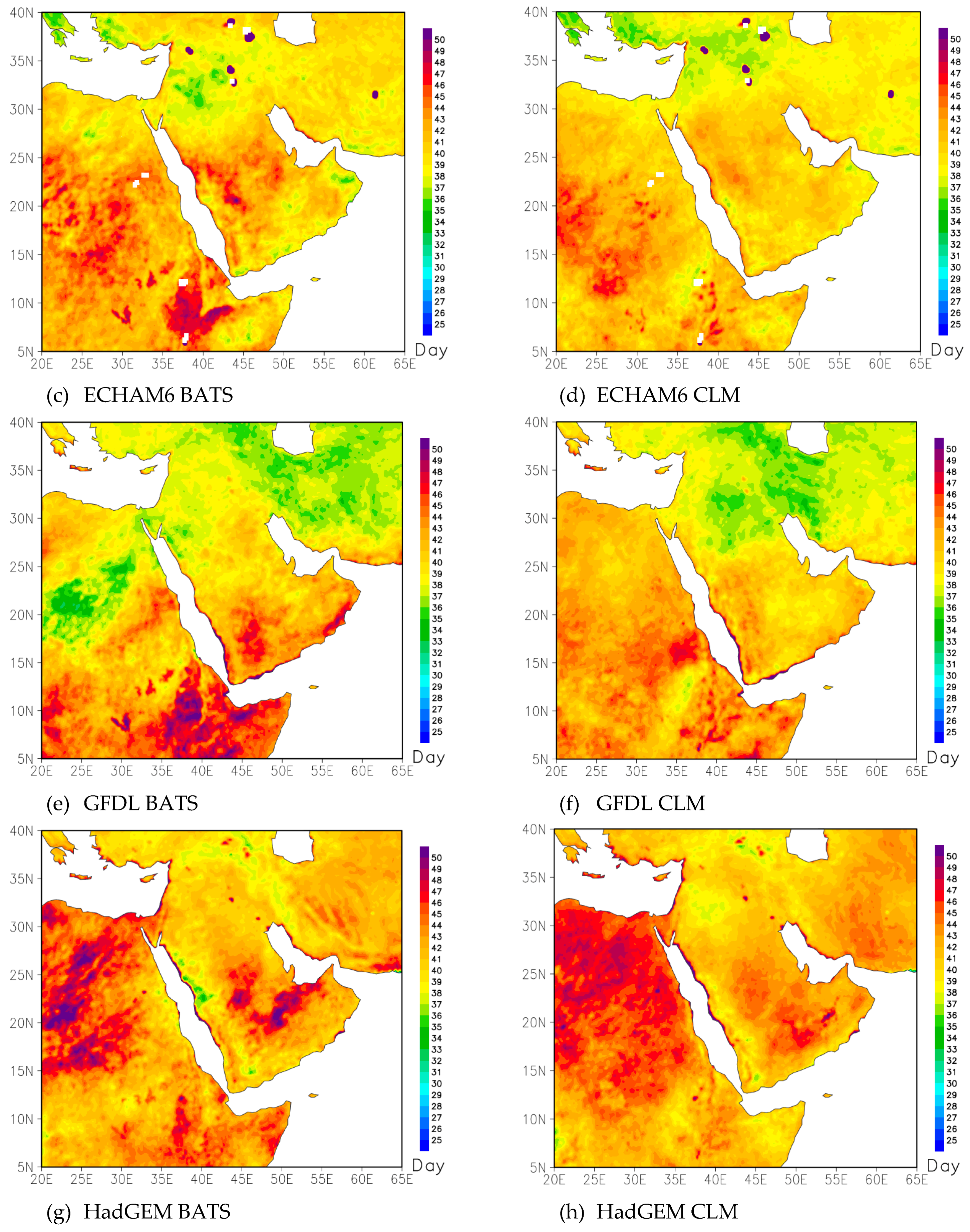
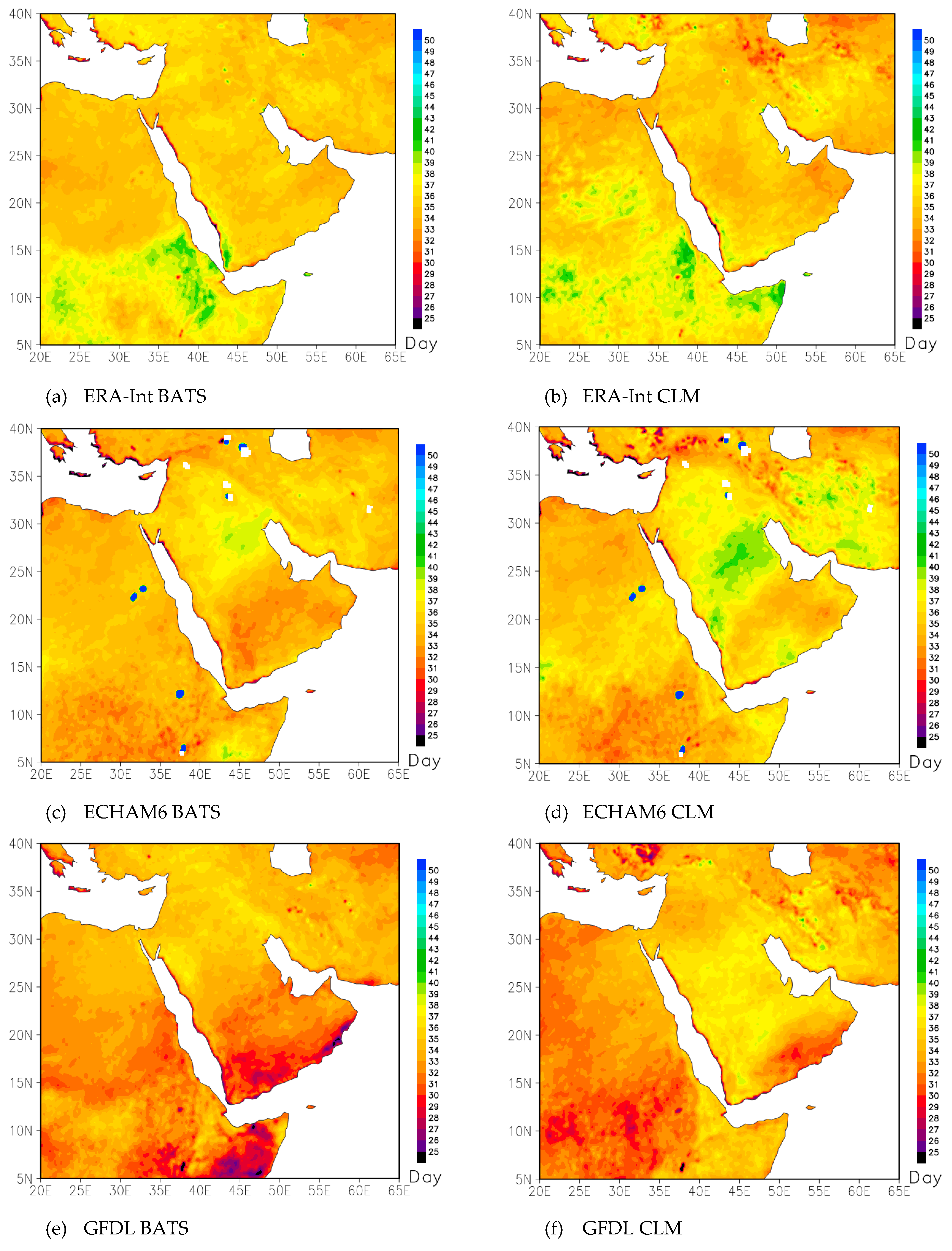
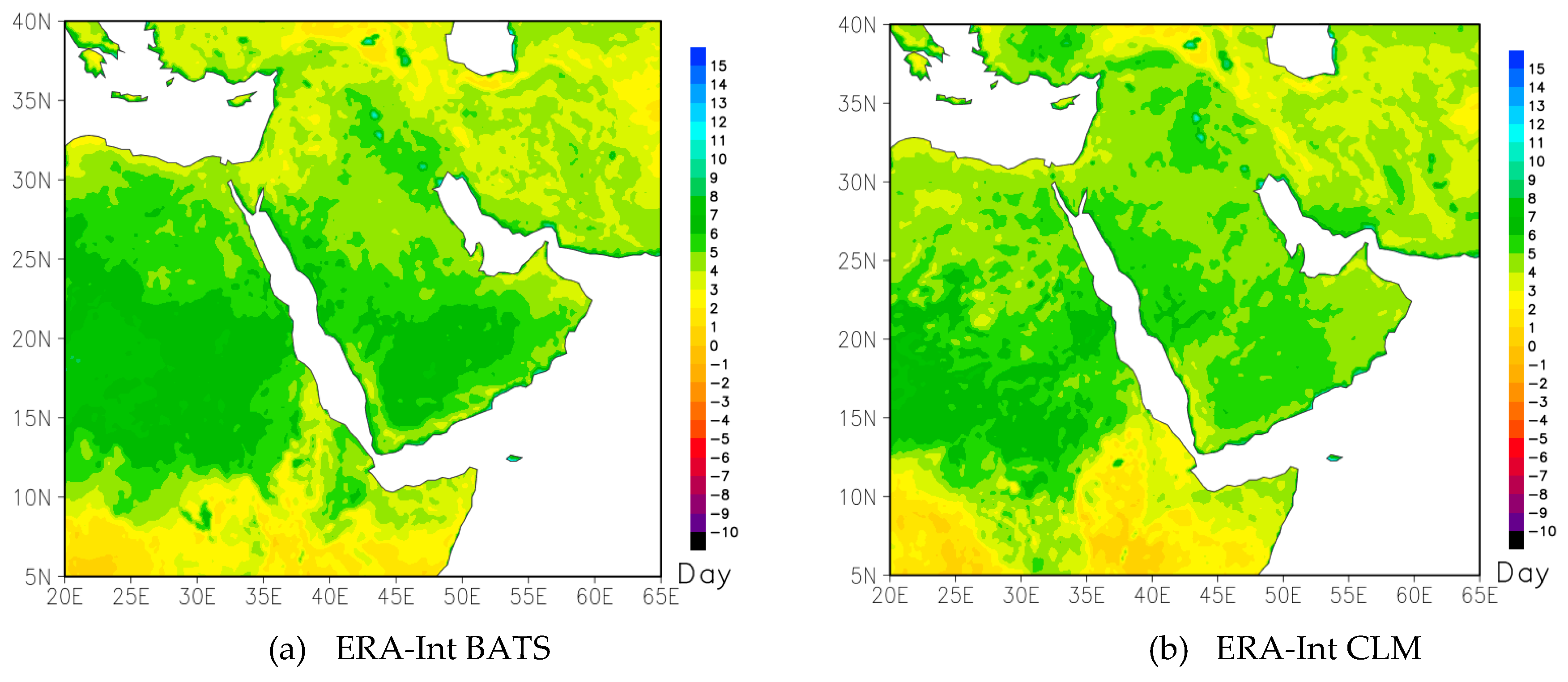
Warm days (TX90p): This index is calculated from daily maximum temperature that varies from region to region over the study area (Figure 4). The BATS simulations show a higher number of warm days compared to the CLM simulations for the period 1986–2005. The number of warm days also varies from the CMIP5 model to model. All the CMIP5 models show a large number of warm days compared to the reanalysis ERA–Int data. Hence, the annual count of warm days ranges from about 30 days to 45 days with reference to the period 1981–2000 over the peninsula.
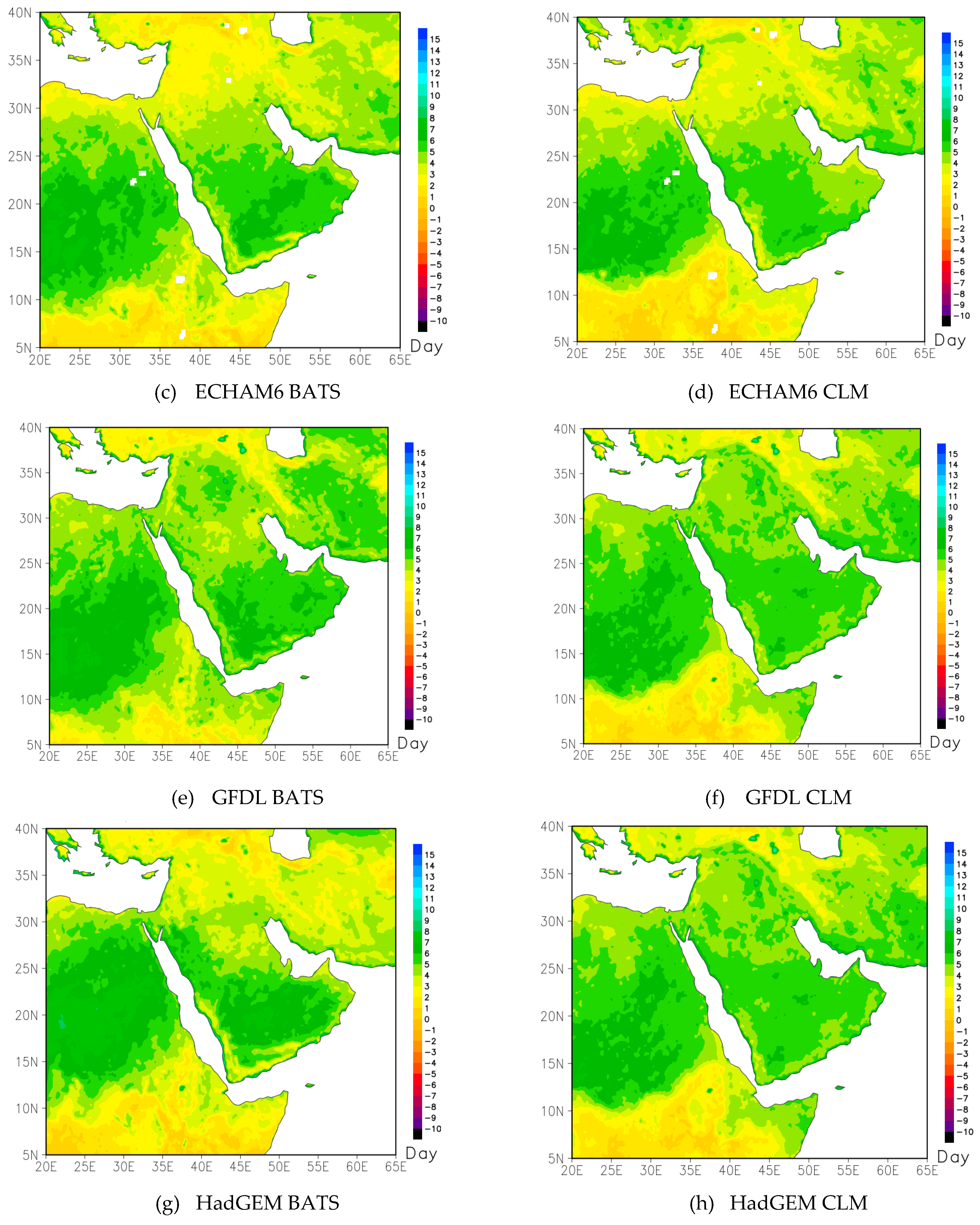
Warm nights (TN90p): This index is calculated from daily minimum temperatures (Figure 5). The TN90p has a similar nature to TX90p in the sense that both vary depending on the place, the model, the land–surface scheme, they show a range of a number of days, and they indicate the warming of the climate of the region. The number of simulated warm nights ranges from about 35 to 45 with reference to the period 1981–2000 over the Arabian Peninsula which is a bit lower than for the ERA–Int. This number of warm nights is somewhat higher than the annual global average of 25 warm nights (Sillmann et al. [17]).
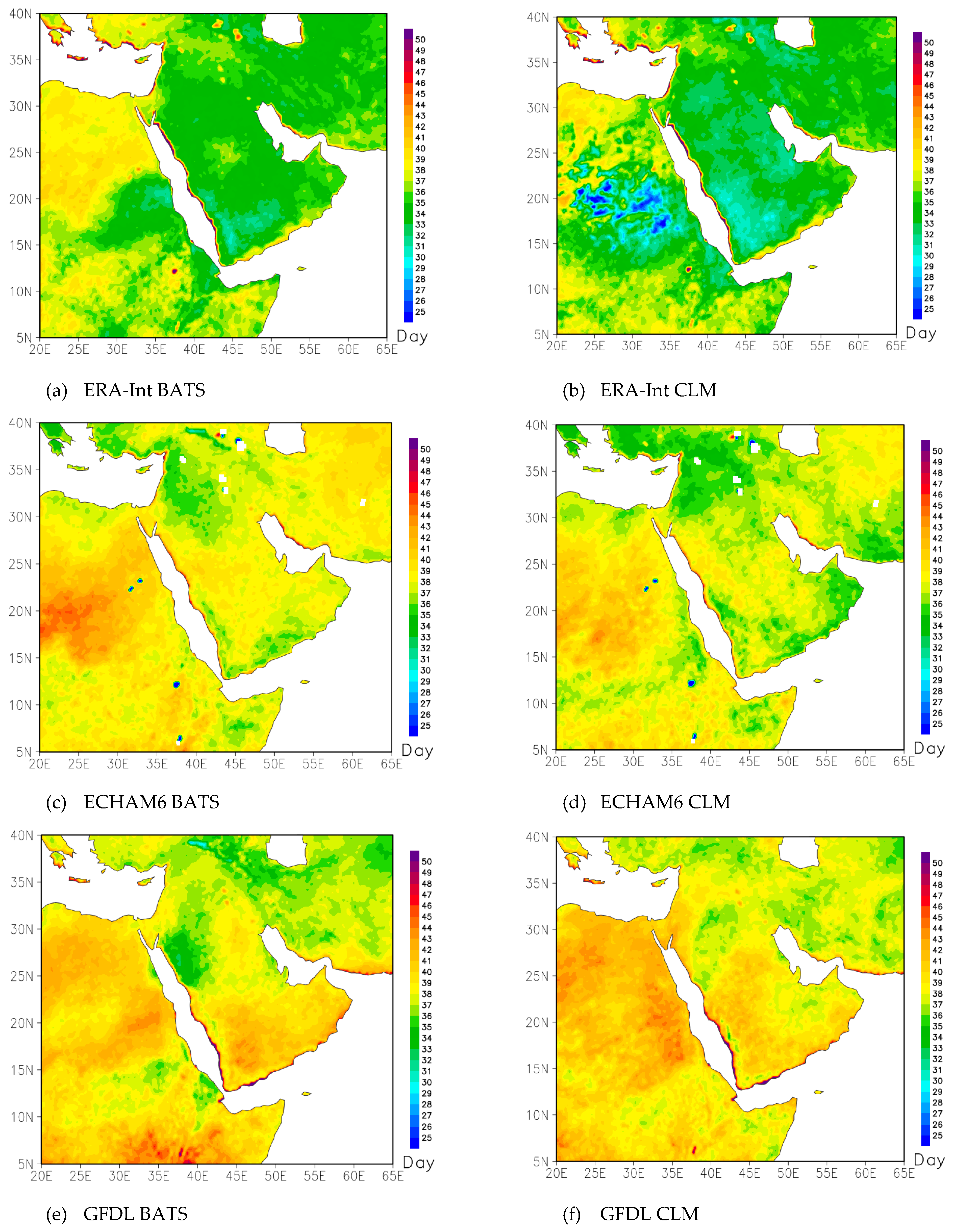
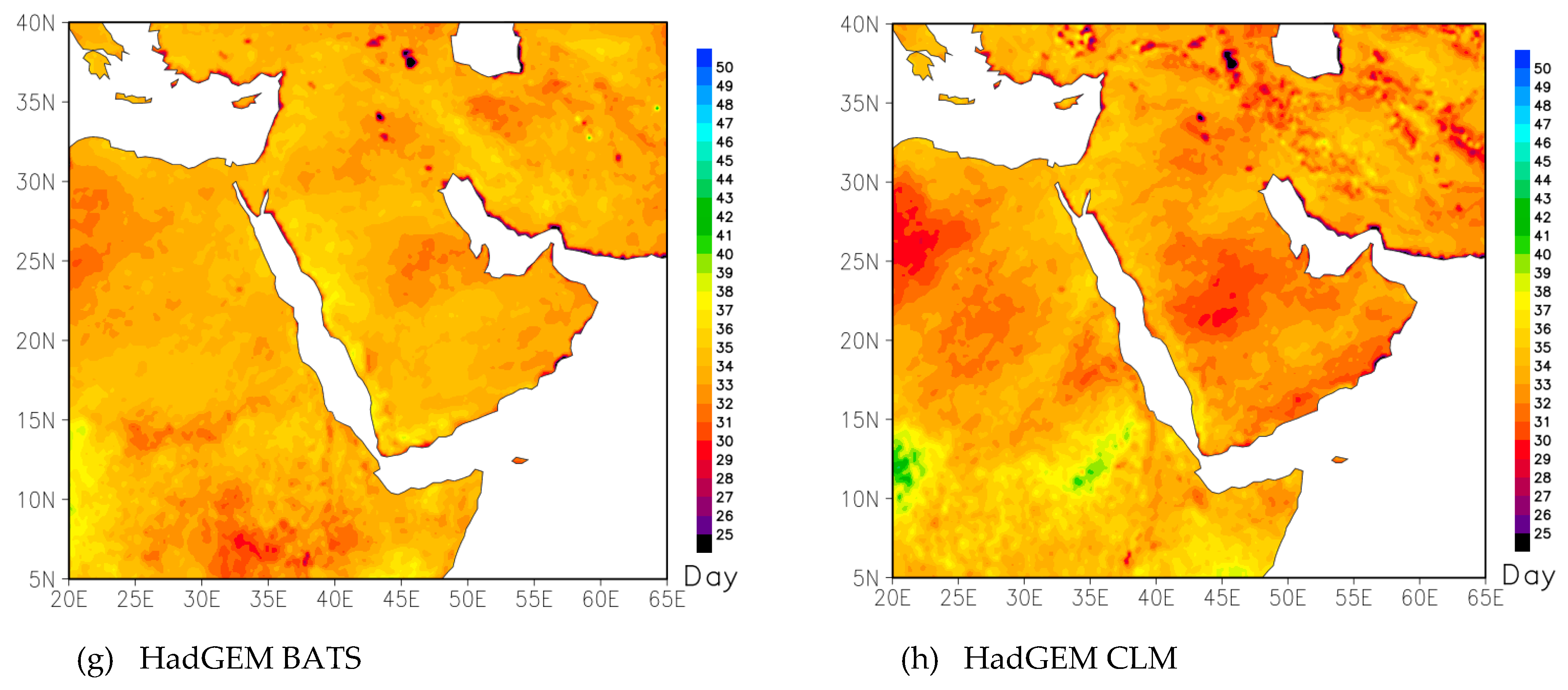
Cold days (TX10p): This index is calculated from the daily maximum temperature from the ERA–Int and CMIP5 models downscaled by RegCM4 (Figure 6). All CMIP5 simulations show the number of TX10p in the range from about 25 to 35 days, which is similar to the ERA–Int result, although ECHAM6 shows the study region to be colder, particularly in the northern part of the peninsula.
Cold nights (TN10p): This index is calculated from daily minimum temperatures in the same way as TX10p (Figure 7). The number of cold nights is slightly lower in CLM simulations than in BATS simulations. Overall, the simulated distribution of cold nights is very similar to the distribution obtained from ERA–Int which is mostly below 38 days. This count is larger than the global annual average of 20 days (Sillmann et al. [17]).
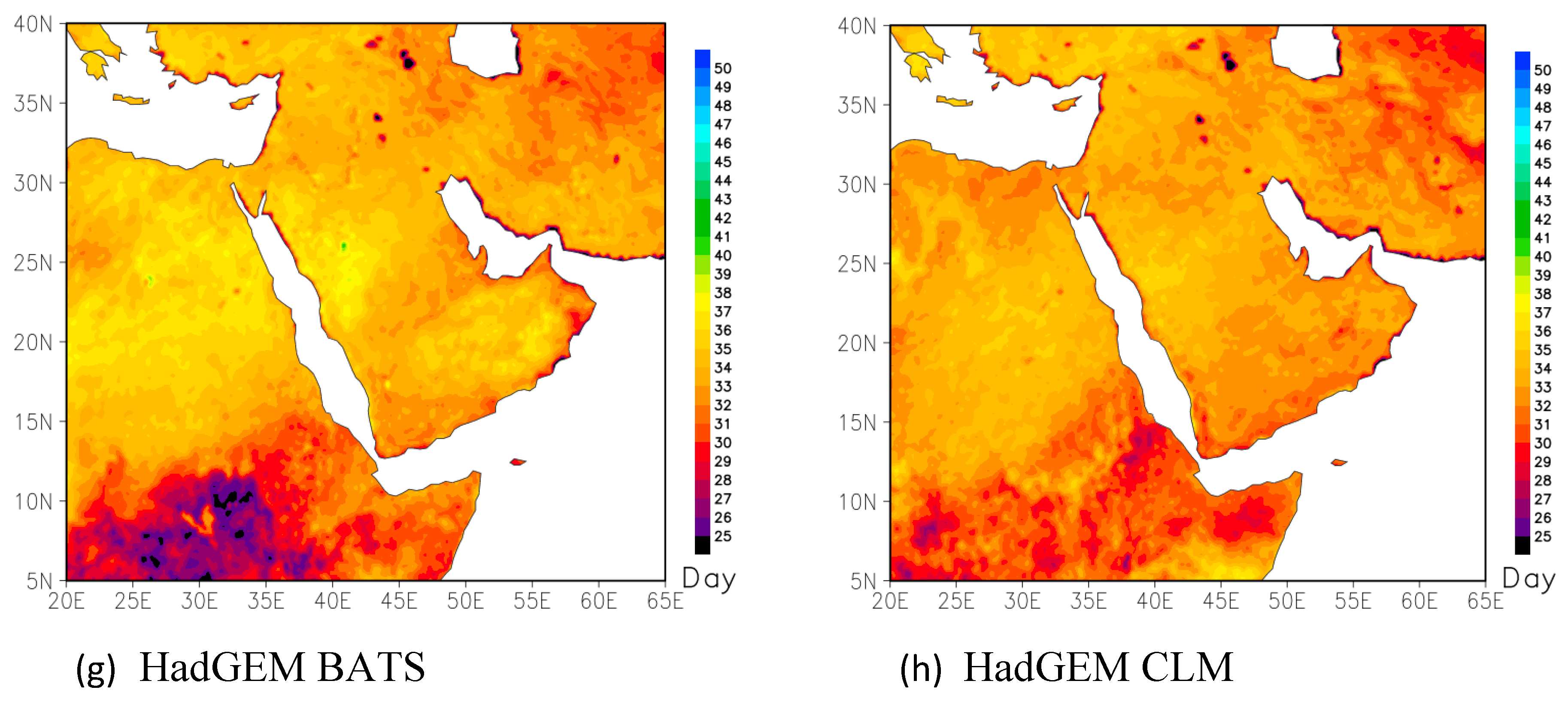
Warm spell duration index (WSDI): This index is calculated from daily maximum temperatures using percentile thresholds relative to the 1981–2000 base period, for the ERA–Int and CMIP5 models (Figure 8). This index varies greatly in space, and RegCM4 with CLM simulated a lower number of WSDI compared to BATS. However, the distribution patterns of the CMIP5 models are very similar to ERA–Int, with a large number of WSDI in the north and a smaller number in the southern part of the study region.
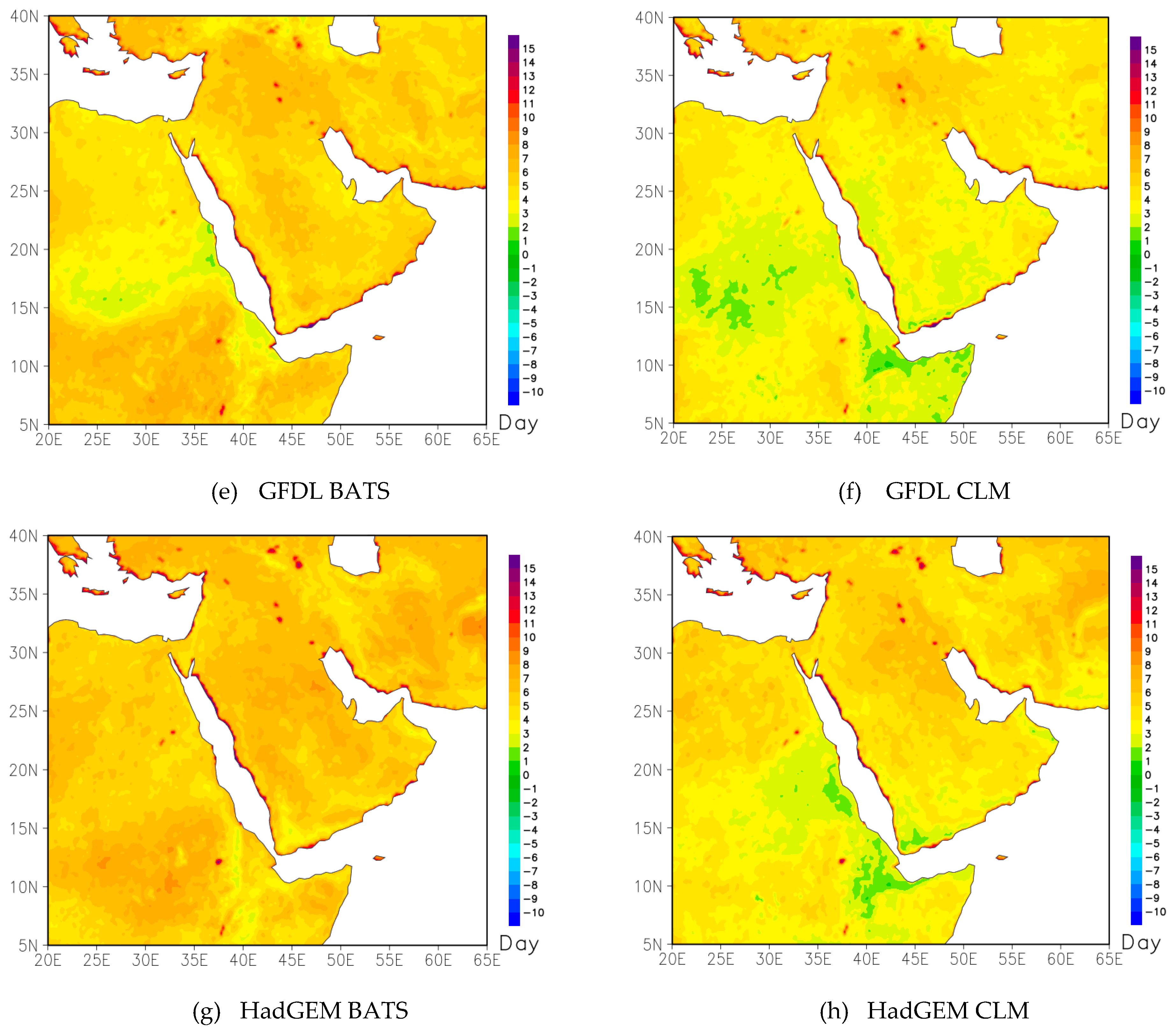
Cold spell duration index (CSDI): This index is calculated from daily minimum temperatures using percentile thresholds relative to the 1981–2000 base period, for the ERA–Int and CMIP5 models (Figure 9). In this case, a large number of CSDI is observed in the south compared to the north of the study region. This lends support to the pattern of WSDI.

3.2.4. Annual Time Series for the Extreme Indices Averaged over the Observational Grids

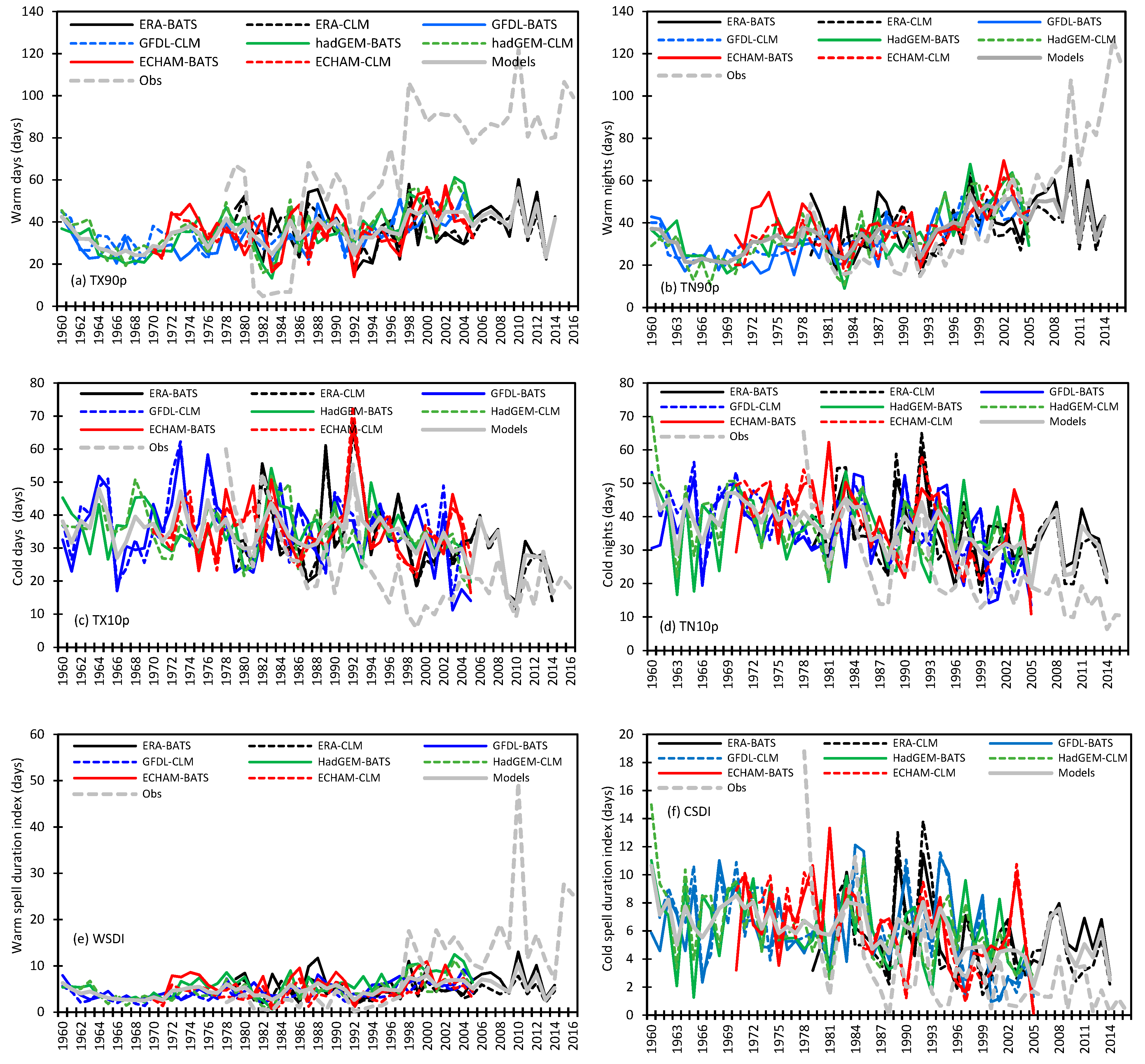
All the simulation–based temperature extreme indices are summarized in Figure 10 along with the observation–based indices for each dataset over the entire period. The trends of the simulation–based temperature extremes closely follow the trends of the observation–based indices although in some cases the magnitudes are slightly different. Irrespective of the different CMIP5 models forcing and land–surface schemes, the warm days/nights show an increasing trend while cold days/nights show a decreasing trend. Moreover, the warm spell duration index is increasing while the cold spell duration index is decreasing. The direction of these increasing and decreasing trends for warm days/nights, cold days/nights and WSDI/CSDI match exactly the global trends (Sillmann et al. [18]). In most cases, the trends are significant (Table 2). Hence, the trends are clear indicators that the climate of the study region is warming and that the CMIP5 data downscaled by RegCM4 captures well the warming trends through the extremes indices calculation. Notably, the average simulation–based temperature extremes trend is in phase with the observation–based temperature extremes trend (columns 12 and 13, Table 2). This statement is also true for the BATS and CLM simulations averaged separately. However, the individual simulations have the same phase as the observed trend, except for ERA–Int reanalysis for TX90p, and ERA–CLM for WSDI. This indicates that the ERA–Int reanalysis does not produce the temperature extreme index (i.e., warm days) correctly in phase with observations. One reason for this might be that the strong positive trend in the observations after 1995 is not well produced by ERA–Int data. Therefore, the overall trend in the observations, and negative in ERA–Int (see Table 2 and Figure 10a). Figure 10 shows that RegCM4 and observation have large differences in temperature indices after 2000. Overall, we can conclude that RegCM4 simulations are able to capture few temperature extremes such as warm days, warm spell duration, and cold nights before 2000 and the RegCM4 simulations do not capture the observed temperature extremes for the entire present climate over the study region.

3.2.5. Precipitation Extremes

Among the 11 precipitation extreme indices obtained from the surface observational data (from the bottom in Table 1), three of them are calculated from RegCM4 simulations as discussed here.
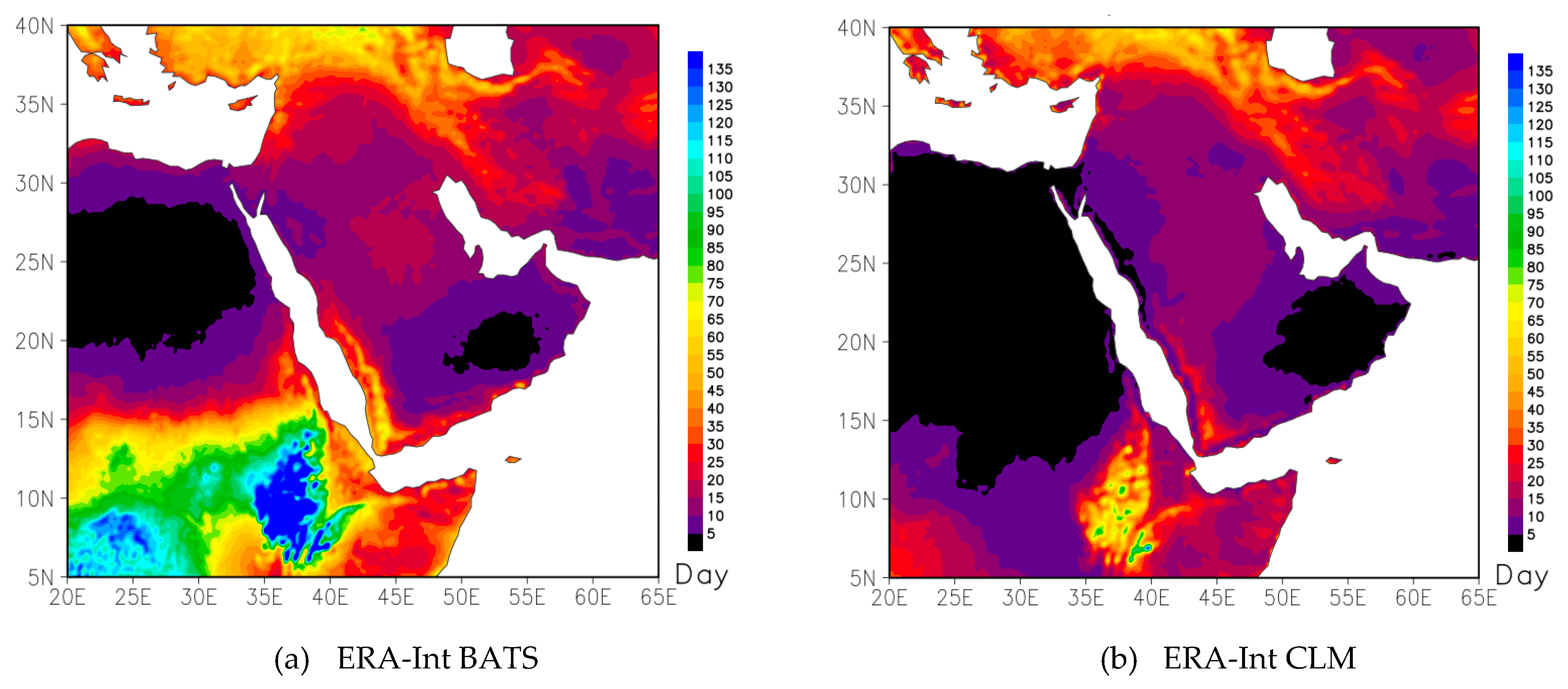
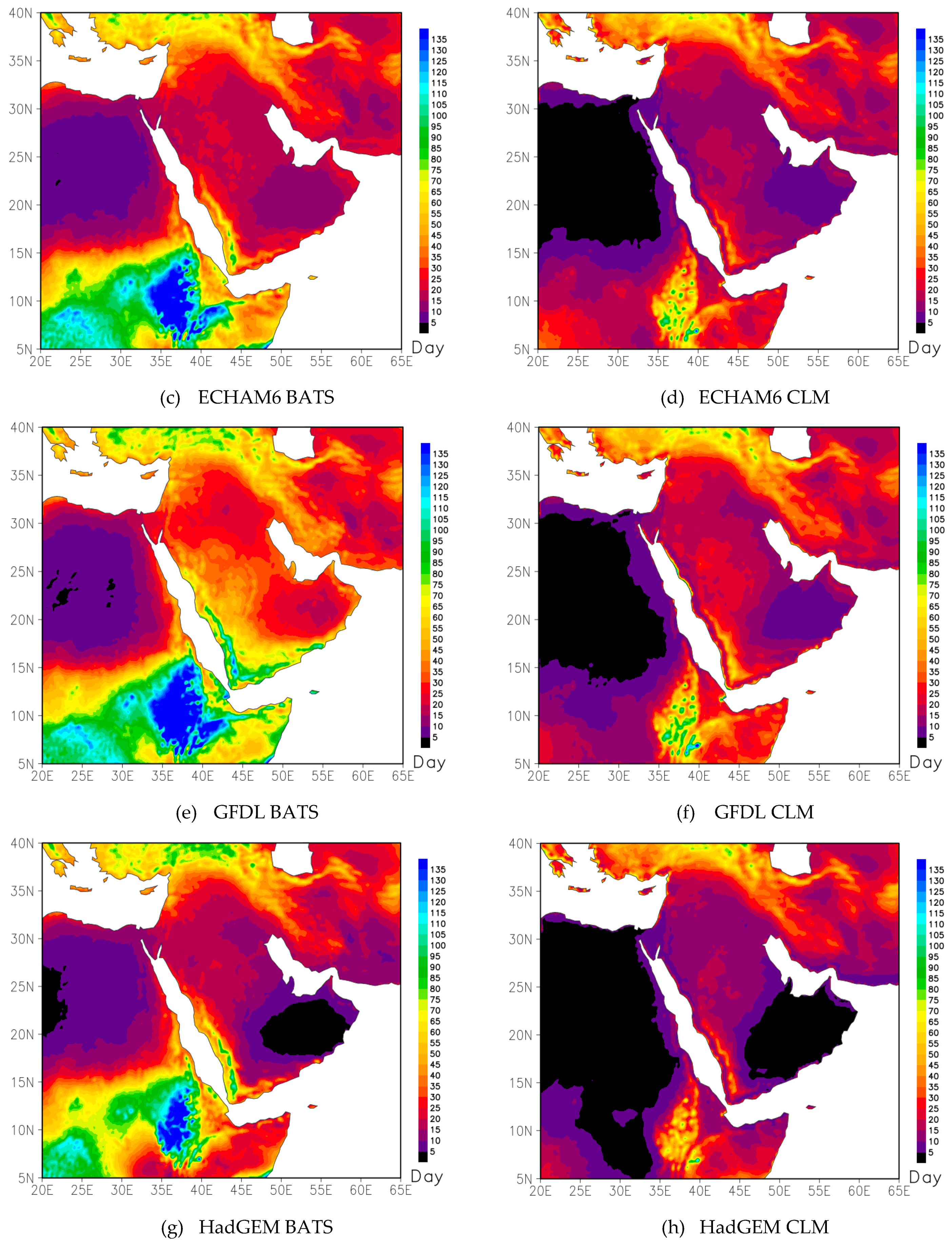
Number of wet days (R1mm): This index is calculated from daily precipitation from the RegCM4 simulations using ERA–Int and CMIP5 data (Figure 11). The absolute value of the R1mm indicates that the number of wet days above 1 mm/day is relatively large (about 45 days per year) over the whole Peninsula except the southeast region, in particular over Oman, UAE, eastern Yemen, and the Rub Al–Khali desert areas where the number of wet days is less than 10. This pattern including the largest number of wet days (about 100) in the southwest region represents the characteristic rainfall distribution over the peninsula. The number of R1mm days is relatively large for the BATS simulation compared to the CLM simulation. Among the simulations, the GFDL case shows a larger number of wet days than the other simulations and a large number than ERA–Int. Overall, the pattern of simulation–based R1mm is similar to that obtained from the ERA–Int forced dataset.
Consecutive wet days (CWD): This index is calculated from daily precipitation amounts from the ERA–Int and CMIP5 models (Figure 12). In general, the number of CWD is low over the peninsula and is lowest in the southeastern area at less than five days. The CWD is highest in the southwestern region of the peninsula. The distribution of CWD absolute values is similar to the distribution of precipitation over the region.
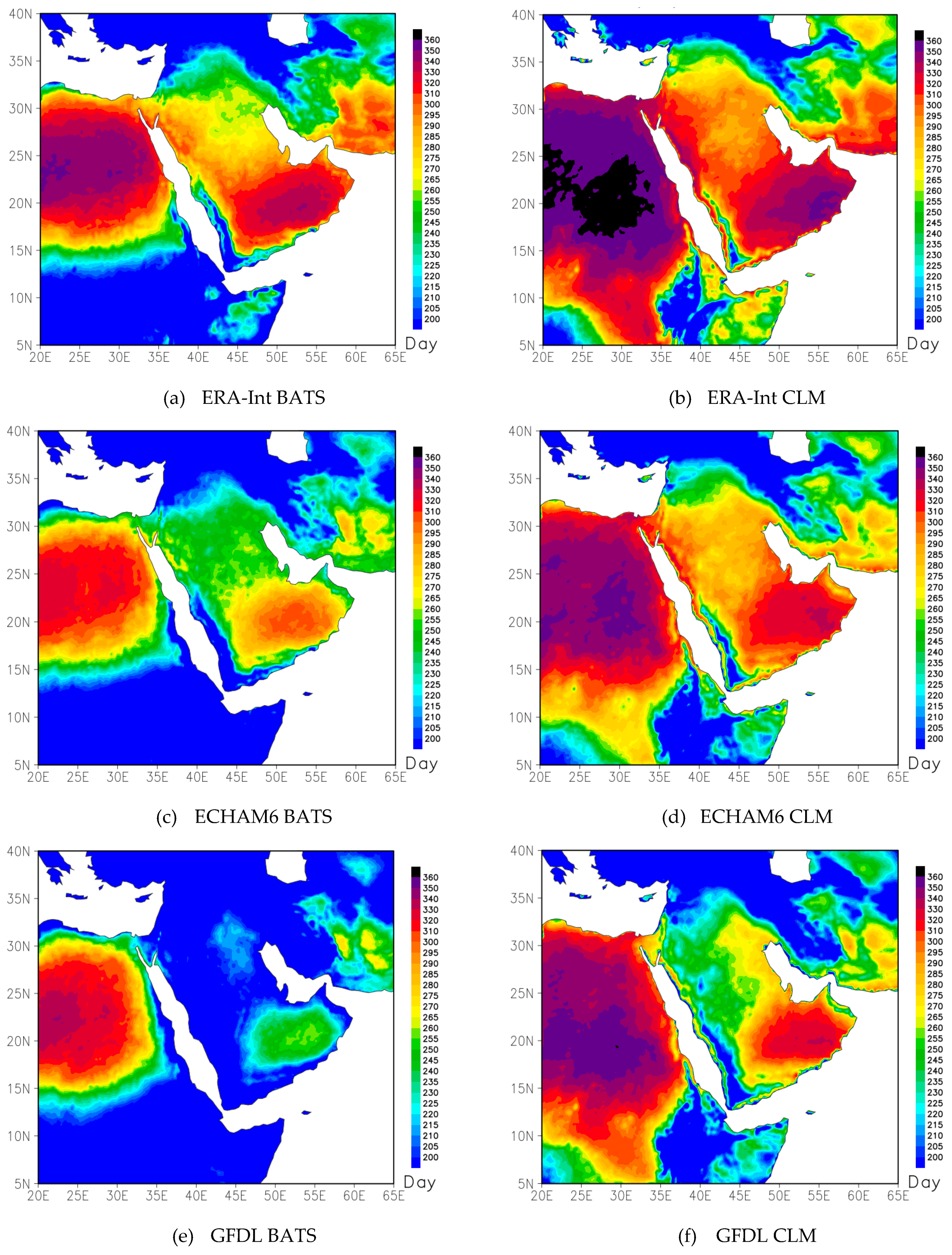
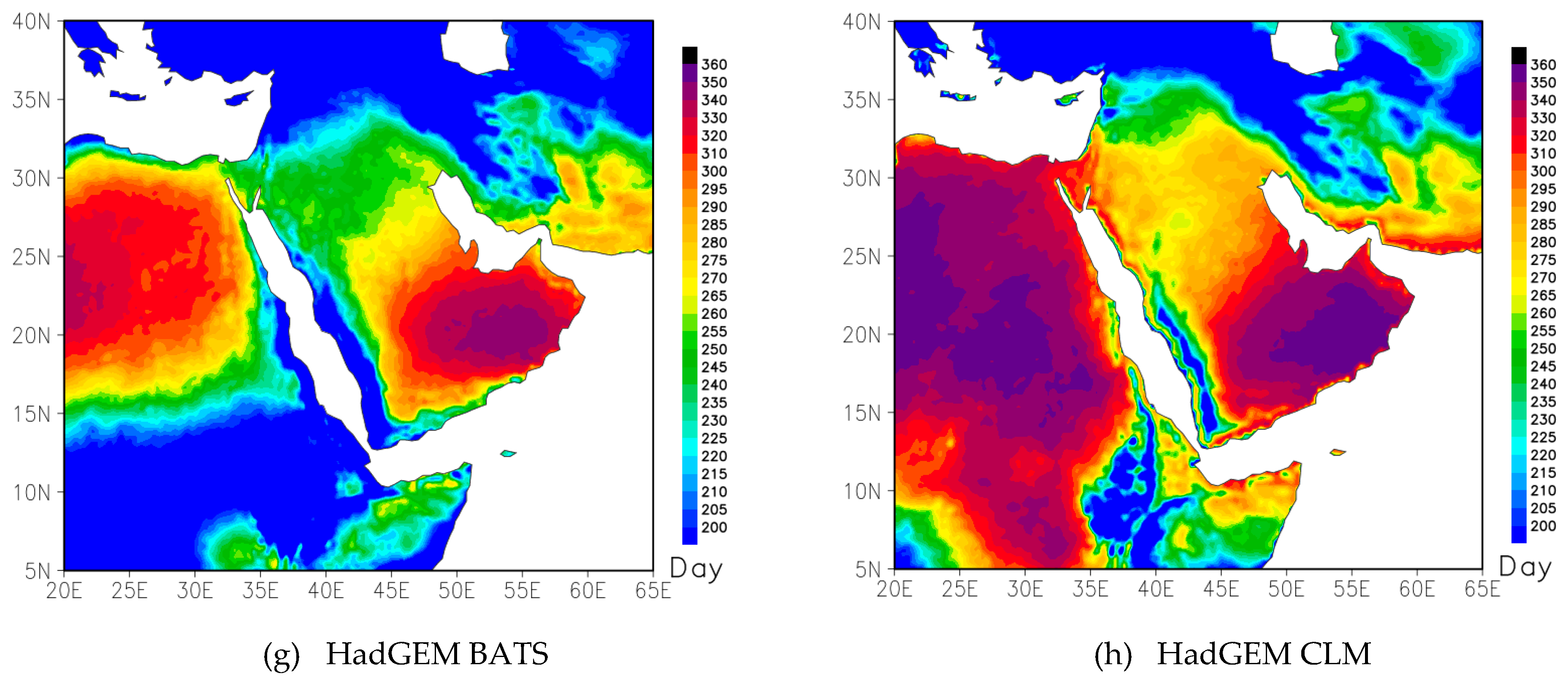
Consecutive dry days (CDD): This index is calculated from daily precipitation amounts from the ERA–Int and CMIP5 models (Figure 13). The absolute value of CDD can reach about 350 days over the Arabian Peninsula, reflecting the arid condition of the region. The CLM simulations produce more consecutive dry days than the BATS simulations, and GFDL produces the fewest CDD compared to other simulations and ERA–Int. The distribution of CDD is similar to the distribution of CWD over the peninsula.
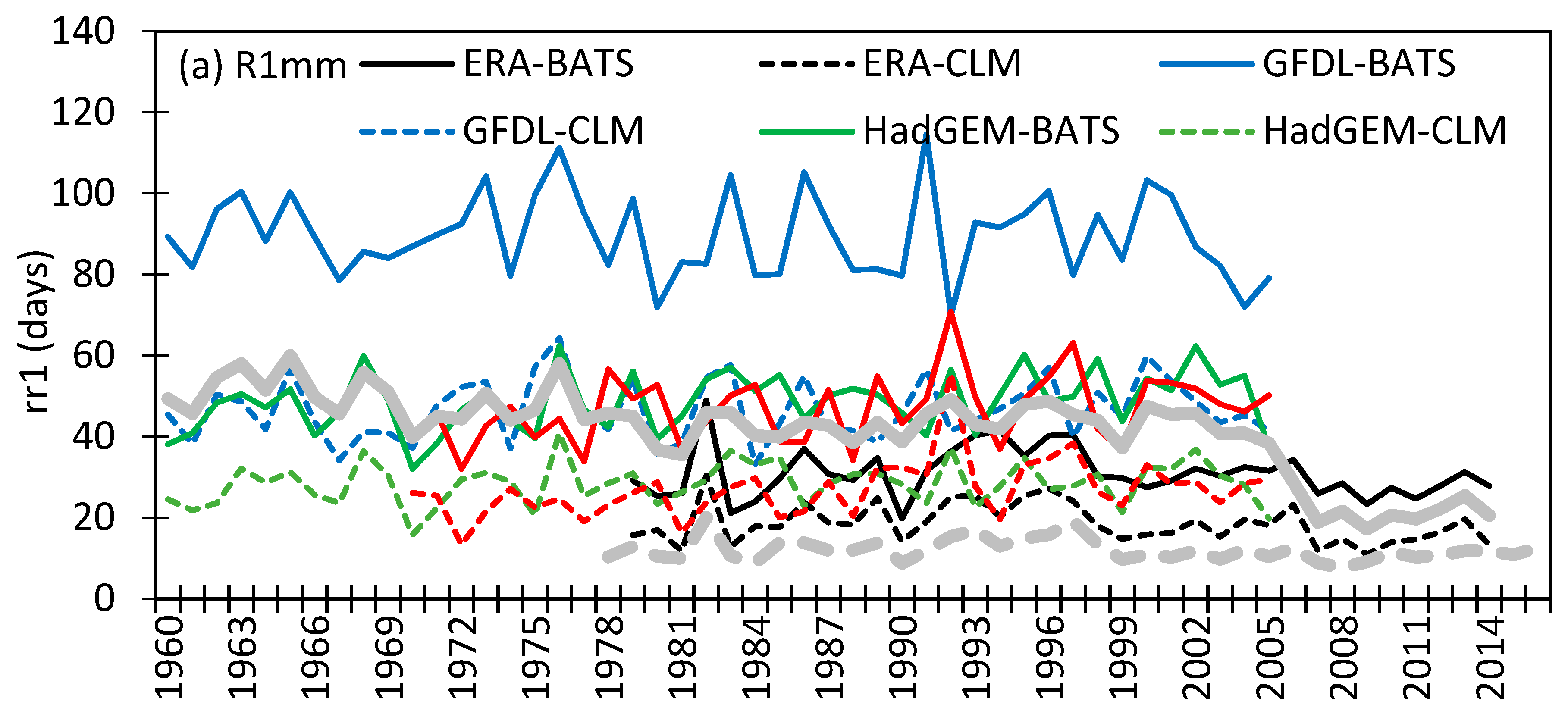
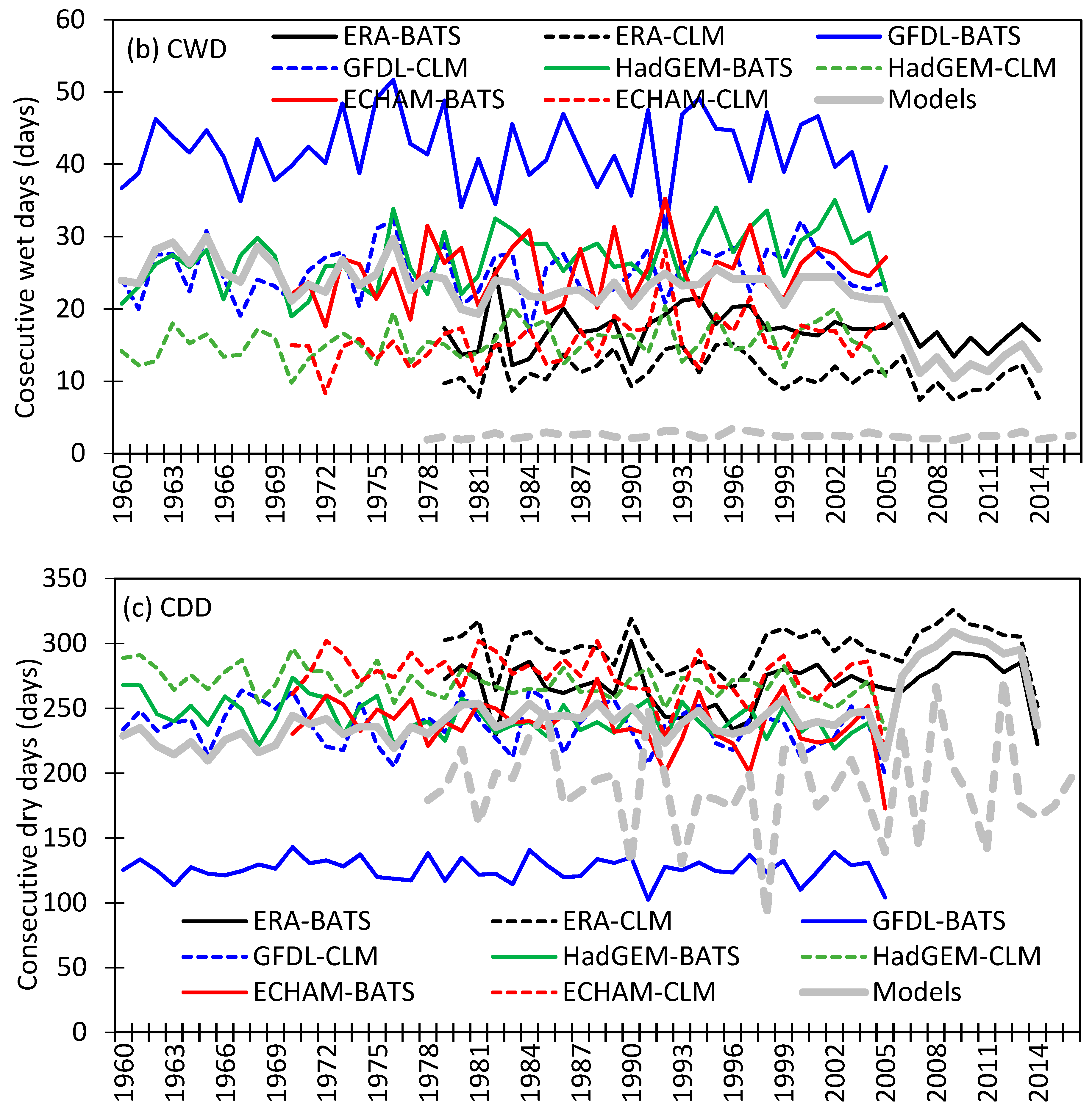
All the simulation–based precipitation extreme indices along with the observation–based indices are summarized in Figure 14. For R1mm, simulation–based extremes indices are overestimated compared to the observations (Figure 14a). The same situation is obtained for the CWD (Figure 14b). In the case of CDD, the simulation–based indices are comparable to observations, although the sharp rise and fall in the observed annual variations are absent in the simulations. The reason is that the number of rainy days is very small and the number of dry days is very large in this study region. Most of the models overestimate precipitation, with consequent false detection of precipitation days. The influence of CDD on a very long dry spell is also mentioned in Sillmann et al. [17]. The magnitude of R1mm, CWD, and CDD also vary greatly from model to model. Overall, the CLM simulations are better able to capture precipitation extremes indices than the BATS simulations, with GFDL–BATS, in particular, being unsuitable.
The summary of the simulation-based precipitation indices indicates that for R1mm, the average trend of the models overall, as well as BATS and CLM individually, is an increasing one, while observations show a decreasing trend (Table 2). The trend of the ERA–Int forced to run with BATS is also in opposition to the observed trend. This also indicates that the ERA–Int reanalysis forced run is not able to provide a precipitation index correctly in phase with the observations. Also [14] mentioned the limitation of reanalysis data in the calculation of precipitation extreme indices. Most of the individual simulations show an opposite trend compared to the observed trend with the exception of the HadGEM–CLM run which shows the same phase and magnitude of the R1mm trend as was measured by observation. ERA–Int with CLM also produces a result in phase with the observed trend. In the case of CDD, all of the simulations and their averages show trends in incorrect phase with the observations. For the CWD, all simulations and their averages show trends in phase with the observed trend. However, HadGEM–CLM, and ERA–Int with CLM produce opposing trends. In most cases, the precipitation trends are insignificant with the exception of a significant trend for CDD (Table 2). Therefore, the use of climate model data when calculating precipitation extreme indices should be done with caution.

3.3. Selection of CMIP5 Models

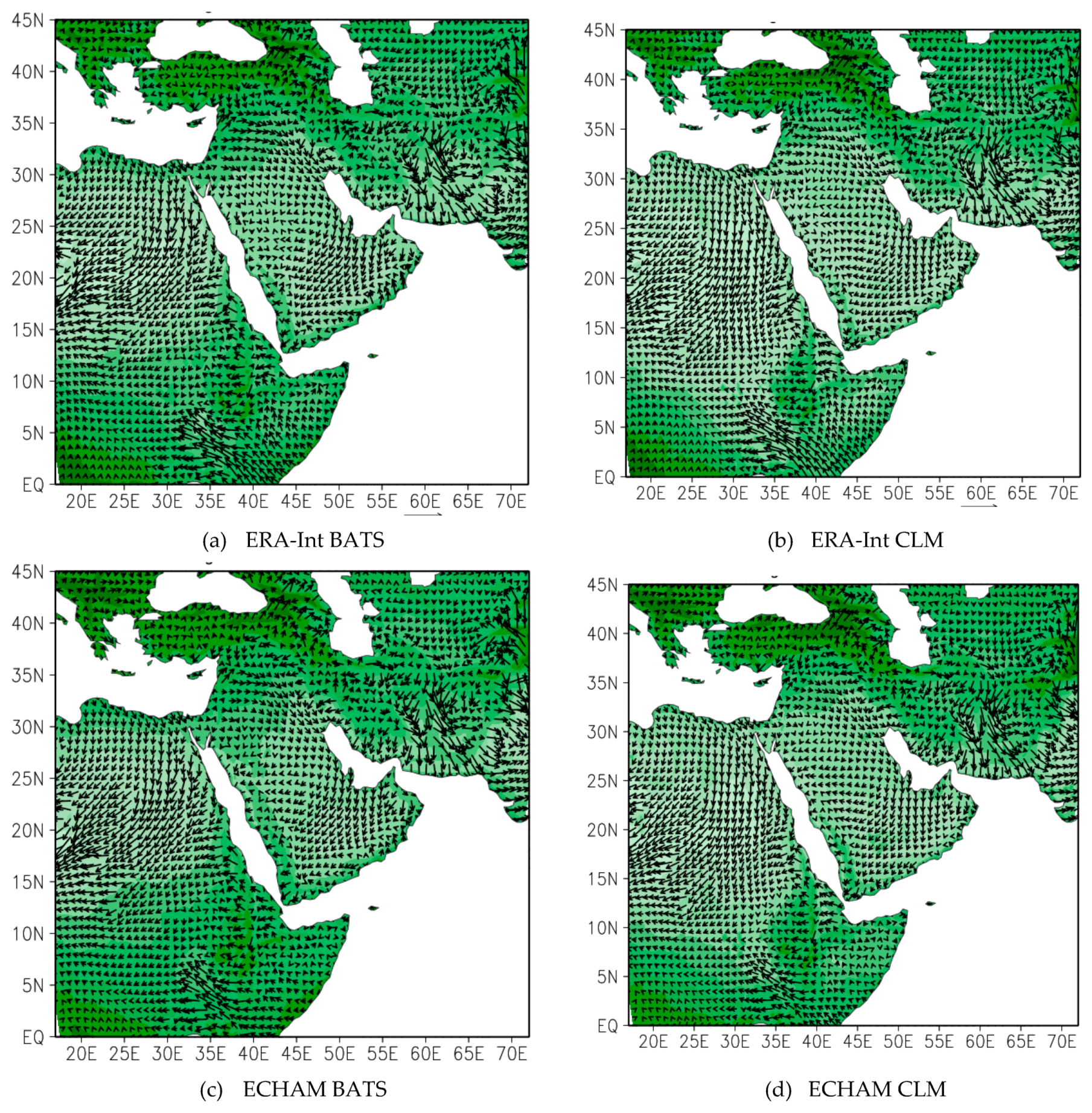
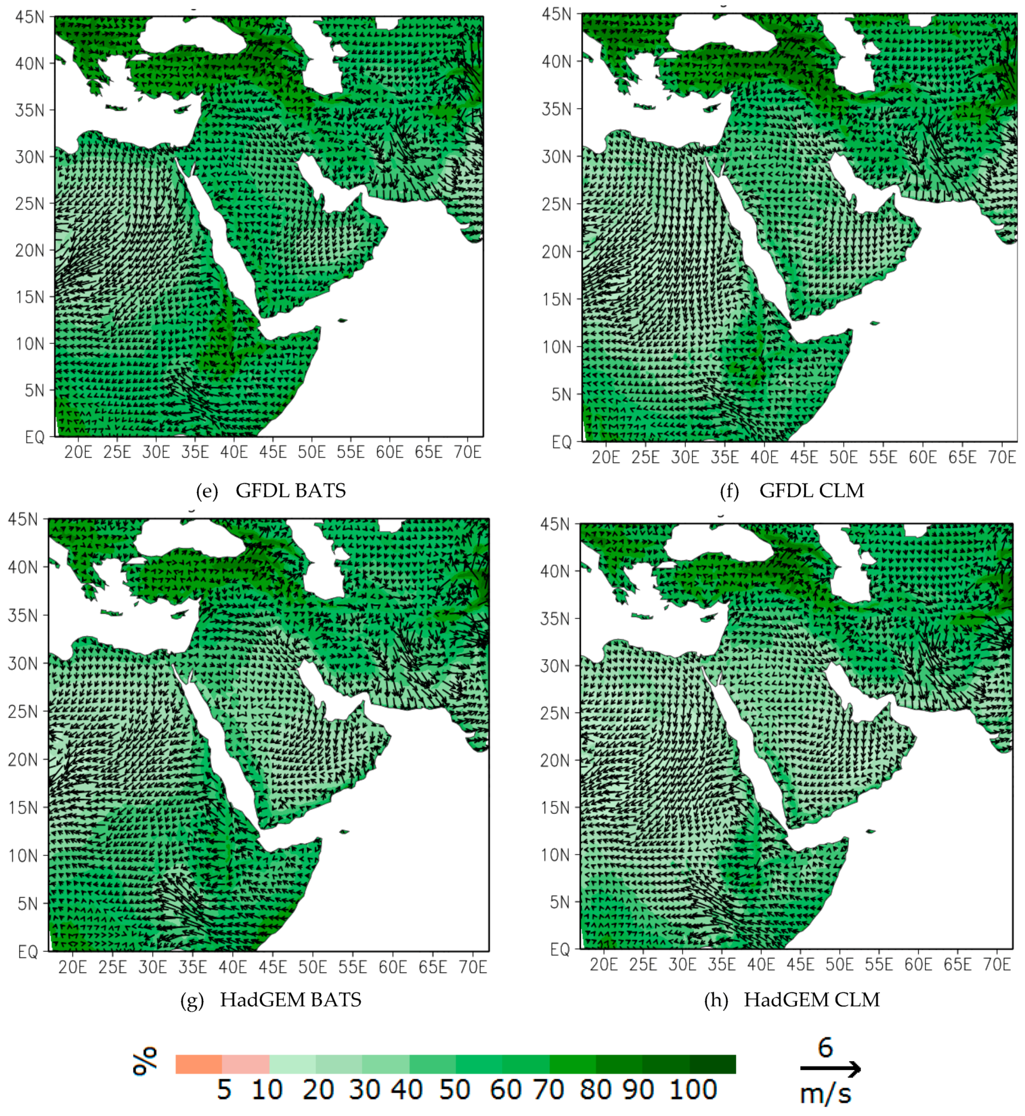
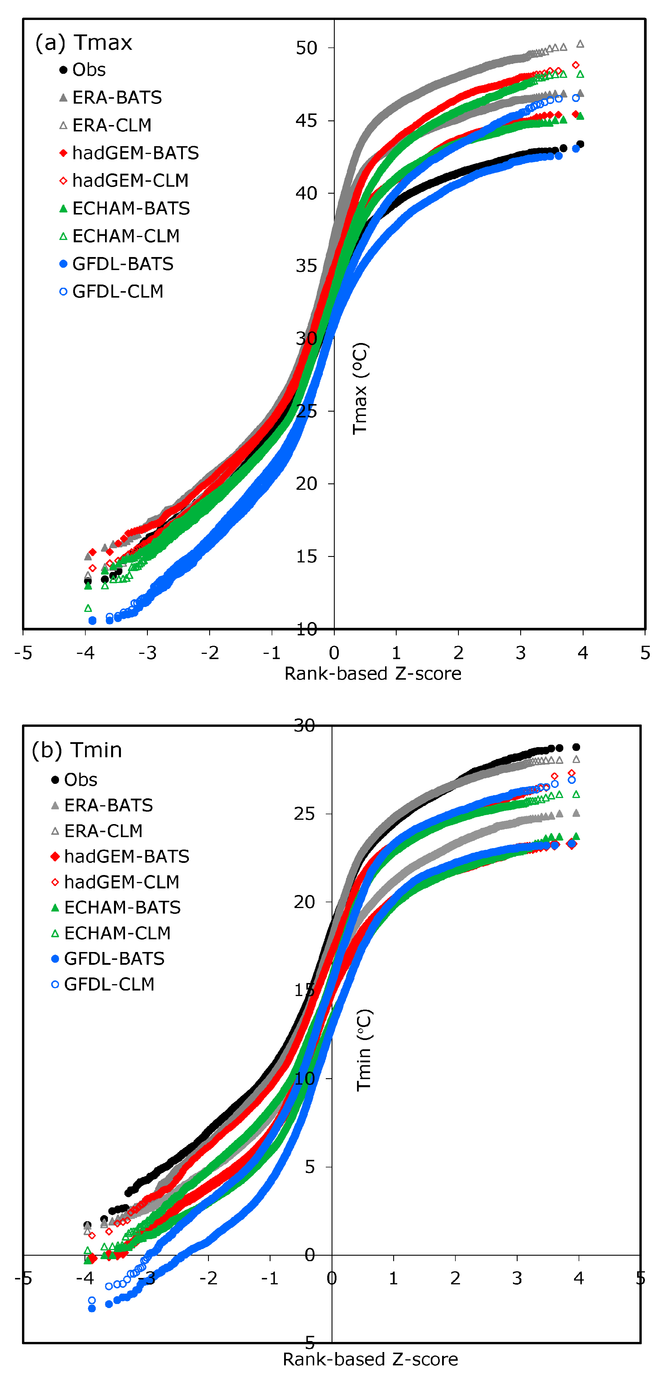
RegCM4 with CLM reproduces relatively weak wind speed and low relative humidity when forced with ERA–Int boundary conditions (Figure 15). The weak wind with low relative humidity is associated with the low precipitation in CLM simulations compared to BATS (Figure 15). The same pattern is noted for all other simulations with CLM and BATS. Among the simulations, the GFDL and HadGEM–forced runs to produce weaker wind field and less humidity than the ERA–Int–forced simulations, while the GFDL–forced run reproduces high humidity. This is one of the reasons that the GFDL-forced simulation overestimates precipitation in the analysis domain. On the other hand, the wind and humidity distribution of the HadGEM forced run is almost identical to the ERA–Int–forced run which simulates similar precipitation from both datasets. The detailed comparison of model performance in simulating temperature and precipitation is obtained through Normal Quantile Plots (Figure 16). Figure 16a clearly shows that for the lower values of maximum temperature, all CMIP5, and ERA–Int reanalysis forced simulations are in line with surface observations with the exception of the GFDL–forced run which largely underestimates the temperature values. The outcome is different for the higher values of maximum temperature, as most of the simulations and ERA–Int overestimate this, with GFDL–BATS the exception in this case reproducing values closer to the observations. The overestimation is evident mainly for summer high-temperature values. Overall, for the low to high values of maximum temperature, ECHAM-BATS, and HadGEM–BATS runs follow a distribution close to the observed one. In the case of minimum temperature, the ERA–Int forced run with CLM reproduces a distribution similar to the observed one, while the HadGEM–CLM, and ECHAM–CLM runs are also close to the observations (Figure 16b). The GFDL-BATS simulation is far from the observations while the GFDL-CLM simulation also significantly deviates from observations far for the lower winter values. It is crucial for any climate model to be able to simulate precipitation on a daily scale. However, the GFDL forced run reproduces values that are too high compared to the observations (Figure 16c). All the other simulations reproduce good distributions compared to observations, although the very high values (about 30 mm/day) are not well captured by any simulation. These results indicate that GFDL is not suitable for present purposes, while HadGEM and ECHAM6 reproduce good simulations of both temperature and precipitation compared to observations on a daily scale. It is interesting to note that these two models are the best performing while GFDL is not the best performing model for the Arabian Peninsula [36]. Hence, better performing models overall also provide better results in climate extremes calculation. For better understanding, a combination of two best-performing models and a weak-performing model are used in this study. Since daily-scale temperature and precipitation data are used in the calculation of extremes indices, the HadGEM and ECHAM6–forced runs are recommended for further use particularly in the calculation of extremes indices in climate projections. The newly developed Saudi-KAU coupled global climate model [30,31] is also a candidate for calculating climate extremes over the study area.

4. Conclusions

In this analysis, the output of three CMIP5 models namely, ECHAM6, GFDL and HadGEM are used as initial and boundary conditions in RegCM4 simulations with the BATS and CLM land–surface schemes in order to calculate climate extremes indices over the Arabian Peninsula for the current period. In an additional simulation, RegCM4 was also forced with the ERA–Int reanalysis data as boundary conditions for the same purpose. The simulation-based extremes indices are compared with the same from an observational dataset obtained from 27 meteorological stations over Saudi Arabia which covers about 85% of the peninsula. First, ETCCDI defined 27 climate extremes indices calculated from observed daily temperature and precipitation data. Among the 27 ETCCDI-based extremes indices, six temperature and three precipitation extremes were calculated using CMIP5 and ERA–Int downscaled data, and were analyzed in detail. Results show that irrespective of the model or land–surface scheme, the temperature extremes are well-captured while, precipitation extreme indices are largely overestimated. All the models can reproduce the trends of temperature extremes in phase with the observations. However, precipitations trends show a mix of results both in phase and out of phase. Only the HadGEM–CLM is able to capture the exact phase and trend of wet days (R1mm). All simulations capture well the phase of CDD trends compared to observations while CWD-simulated trends are captured by most of the simulations with the exceptions of Had-CLM and ERA–Int CLM. Therefore, the model-simulated daily data can be used to calculate temperature extremes indices for the future climate while the use of this daily data in the calculation of precipitation extremes indices should be done with more precaution. Of the three CMIP5 models outputs downscaled by RegCM4 in this analysis, the best performing are HadGEM and ECHAM6-based simulations. These provide data that are recommended in the examination of extremes indices for the projection period, while the less-well performing GFDL model is not recommended.

Supplementary Materials

The following are available online at https://www.mdpi.com/2073-4433/10/11/675/s1, Figure S1: Spatial distribution of maximum temperature bias (C°) with reference to the CRU data for (a) ERA-Int BATS, (b) ERA-Int CLM, (c) ECHAM6 BATS, (d) ECHAM6 CLM, (e) GFDL BATS, (f) GFDL CLM, (g) HadGEM BATS, and (h) HadGEM CLM averaged over the period 1980–2005, Figure S2: Spatial distribution of minimum temperature bias (C°) with reference to the CRU data for (a) ERA-Int BATS, (b) ERA-Int CLM, (c) ECHAM6 BATS, (d) ECHAM6 CLM, (e) GFDL BATS, (f) GFDL CLM, (g) HadGEM BATS, and (h) HadGEM CLM averaged over the period 1980–2005, Figure S3: Spatial distribution of precipitation bias (%) with reference to the CRU data for (a) ERA-Int BATS, (b) ERA-Int CLM, (c) ECHAM6 BATS, (d) ECHAM6 CLM, (e) GFDL BATS, (f) GFDL CLM, (g) HadGEM BATS, and (h) HadGEM CLM averaged over the period 1980–2005.

Funding

This research received no external funding.

Acknowledgments

The author would like to acknowledge the General Authority of Meteorology and Environmental Protection (GAMEP) for providing surface observations and ICTP, Trieste, Italy, is acknowledged for providing the RegCM4. The CRU, ERA–Int and CMIP5 data were acquired from their websites. Computation for the work described in this paper was performed using Aziz Supercomputer at King Abdulaziz University’s High Performance Computing Center, Jeddah, Saudi Arabia.

Conflicts of Interest

The authors declare no conflict of interest.

References

  1. Sun, Q.; Miao, C.; Duan, Q. Extreme climate events and agricultural climate indices in China: CMIP5 model evaluation and projections. Int. J. Climatol. 2016, 36, 43–61. [Google Scholar] [CrossRef]
  2. IPCC. A Special Report of Working Groups I and II of the Intergovernmental Panel on Climate Change: Managing the Risks of Extreme Events and Disasters to Advance Climate Change Adaptation–Summary for Policymakers; Cambridge University Press: Cambridge, UK, 2013. [Google Scholar]
  3. IPCC. Climate Change 2007. The Physical Sciences Basis Contribution of Working Group 1 to the Fourth Assessment Report of the Intergovernmental Panel on Climate Change; Solomon, S., Qin, D., Manning, M., Chen, Z., Marquis, M., Averyt, K.B., Tignor, M., Miller, H.L., Eds.; Cambridge University Press: Cambridge, UK, 2007; p. 4. [Google Scholar]
  4. Almazroui, M.; Islam, M.N.; Athar, H.; Jones, P.D.; Rahman, M.A. Recent climate change in the Arabian Peninsula: Annual rainfall and temperature analysis of Saudi Arabia for 1978–2009. Int. J. Climatol. 2012, 32, 953–966. [Google Scholar] [CrossRef]
  5. Almazroui, M.; Islam, M.N.; Jones, P.D. Urbanization effects on the air temperature rise in Saudi Arabia. Clim. Chang. 2013, 120, 109–122. [Google Scholar] [CrossRef]
  6. Almazroui, M. Temperature changes over the CORDEX-MENA domain in the 21st century using CMIP5 data downscaled with RegCM4: A focus on the Arabian Peninsula. Advan. Meteorol. 2019, 18. [Google Scholar] [CrossRef]
  7. Atif, R.M.; Almazroui, M.; Saeed, S.; Abid, M.A.; Islam, M.N.; Ismail, M. Extreme precipitation events over Saudi Arabia during the wet season and their associated teleconnections. Atmos. Res. 2019, 231, 104655. [Google Scholar] [CrossRef]
  8. Saeed, S.; Almazroui, M. Impacts of mid-latitude circulation on winter precipitation over the Arabian Peninsula. Clim. Dyn. 2019. [Google Scholar] [CrossRef]
  9. Almazroui, M.; Saeed, S. Contribution of extreme daily precipitation to total rainfall over the Arabian Peninsula. Atmos. Res. 2019. [Google Scholar] [CrossRef]
  10. Easterling, D.; Meehl, G.A.; Parmesan, C.; Changnon, S.A.; Karl, T.R.; Mearns, L.O. Climate Extremes: Observations, Modeling, and Impacts. Science 2000, 289, 2068–2074. [Google Scholar] [CrossRef] [Green Version]
  11. AlSarmi, S.H.; Washington, R. Review Changes in climate extremes in the Arabian Peninsula: Analysis of daily data. Int. J. Climatol. 2013, 34, 1329–1345. [Google Scholar] [CrossRef]
  12. Almazroui, M.; Islam, M.N.; Dambul, R.; Jones, P.D. Trends of temperature extremes in Saudi Arabia. Int. J. Climatol. 2014, 34, 808–826. [Google Scholar] [CrossRef]
  13. Donat, M.G.; Peterson, T.C.; Brunet, M.; King, A.D.; Almazroui, M.; Kolli, R.K.; Boucherf, D.; Al-Mulla, A.Y.; Nour, A.Y.; Aly, A.A.; et al. Changes in extreme temperature and precipitation in the Arab region: Long-term trends and variability related to ENSO and NAO. Int. J. Climatol. 2014, 34, 581–592. [Google Scholar] [CrossRef]
  14. Islam, M.N.; Almazroui, M.; Dambul, R.; Jones, P.D.; Alamoudi, A.O. Long-term changes in seasonal temperature extremes over Saudi Arabia during 1981–2010. Int. J. Climatol. 2015, 35, 1579–1592. [Google Scholar] [CrossRef]
  15. You, Q.; Ren, G.; Fraedrich, K.; Kang, S.; Ren, Y.; Wang, P. Winter temperature extremes in China and their possible Causes. Int. J. Climatol. 2013, 33, 1444–1455. [Google Scholar] [CrossRef]
  16. Alexander, L.V.; Zhang, X.; Peterson, T.C.; Caesar, J.; Gleason, B.; Klein Tank, A.M.G.; Haylock, M.; Collins, D.; Trewin, B.; Rahimzadeh, F.; et al. Global observed changes in daily climate extremes of temperature and precipitation. J. Geophy. Res. 2006, 111, D05109. [Google Scholar] [CrossRef]
  17. Sillmann, J.; Kharin, V.V.; Zhang, X.; Zwiers, F.W.; Bronaugh, D. Climate extremes indices in the CMIP5 multimodel ensemble: Part 1. Model evaluation in the present climate. J. Geophy. Res. Atmos. 2013, 118, 1716–1733. [Google Scholar] [CrossRef]
  18. Sillmann, J.; Kharin, V.V.; Zwiers, F.W.; Zhang, X.; Bronaugh, D. Climate extremes indices in the CMIP5 multimodel ensemble: Part 2. Future climate projections. J. Geophy. Res. Atmos. 2013, 118, 2473–2493. [Google Scholar] [CrossRef]
  19. Tank, A.M.G.; Zwiers, F.W.; Zhang, X. Guidelines on Analysis of Extremes in a Changing Climate in Support of Informed Decisions for Adaptation; Climate Data and Monitoring 2009, WCDMP-No. 72. World Meteorological Organization WMO-TD No. 1500; World Meteorological Organization: Geneva, Switzerland, 2009. [Google Scholar]
  20. Karl, T.R.; Easterling, D. Climate Extremes: Selected Review and Future Research Directions. Clim. Chang. 1999, 42, 309–325. [Google Scholar] [CrossRef]
  21. Revadekar, J.V.; Hameed, S.; Collins, D.; Manton, M.; Sheikh, M.M.; Borgaonkar, H.P.; Kothawale, D.R.; Adnan, M.; Ahmed, A.U.; Ashraf, J.; et al. Impact of altitude and latitude on changes in temperature extremes over South Asia during 1971–2000. Int. J. Climatol. 2012, 33, 192–209. [Google Scholar] [CrossRef]
  22. Wheeler, T.; Braun, v.J. Climate Change Impacts on Global Food Security. Science 2013, 341, 508–513. [Google Scholar] [CrossRef]
  23. Tsikerdekis, A.; Zanis, P.; Georgoulias, A.K.; Alexandri, G.; Katragkou, E.; Karacostas, T.; Solmon, F. Direct and semi-direct radiative effect of North African dust in present and future regional climate simulations. Clim. Dyn. 2019, 53, 4311–4336. [Google Scholar] [CrossRef]
  24. Giorgi, F.; Coppola, E.; Solmon, F.; Mariotti, L.; Sylla, M.B.; Bi, X.; Elguindi, N.; Diro, G.T.; Nair, V.; Giuliani, G.; et al. RegCM4: Model description and preliminary tests over multiple CORDEX domains. Clim. Res. 2012, 52, 7–29. [Google Scholar] [CrossRef]
  25. Gao, X.; Pal, J.S.; Giorgi, F. Projected changes in mean and extreme precipitation over the Mediterranean region from a high resolution double nested RCM simulation. Geophy. Res. Lett. 2006, 33, L03706. [Google Scholar] [CrossRef]
  26. Dickinson, R.E.; Henderson-Sellers, A.; Kennedy, P.J. Biosphere-atmosphere transfer scheme (BATS) version 1 as coupled to the NCAR community climate model. Note TH-387+ STR Natl. Cent. Atmos. Res. 1993. [Google Scholar] [CrossRef]
  27. Oleson, K.W.; Niu, G.Y.; Yang, Z.L. Improvements to the Community Land Model and their impact on the hydrological cycle. J. Geophys. Res. 2008, 113. [Google Scholar] [CrossRef]
  28. Steiner, A.L.; Pal, J.S.; Giorgi, F.; Dickinson, R.E.; Chameides, W.L. The coupling of the Common Land Model (CLM0) toaregional climate model (RegCM). Theor. Appl. Climatol. 2005. [Google Scholar] [CrossRef]
  29. Fritsch, J.M.; Chappell, C.F. Numerical prediction of convectively driven mesoscale pressure systems, Part I, Convective parameterization. J. Atmos. Sci. 1980, 37, 1722–1733. [Google Scholar] [CrossRef]
  30. Fritsch, J.M.; Chappell, C.F. Numerical Prediction of Convectively Driven Mesoscale Pressure Systems, Part II, Mesoscale Model. J. Atmos. Sci. 1980, 37, 1734–1762. [Google Scholar] [CrossRef]
  31. Islam, M.N.; Almazroui, M. Direct effects and feedback of desert dust on the climate of the Arabian Peninsula during the wet season: A regional climate model study. Clim. Dyn. 2012, 39, 2239–2250. [Google Scholar] [CrossRef]
  32. Harris, I.; Jones, P.D.; Osborn, T.J.; Lister, D. Updated high-resolution grids of monthly climatic observations—The CRU TS3.10 Dataset. Int. J. Climatol. 2014, 34, 623–642. [Google Scholar] [CrossRef]
  33. Almazroui, M.; Islam, M.N.; Saeed, S.; Alkhalaf, A.K.; Dambul, R. Assessment of Uncertainties in Projected Temperature and Precipitation over the Arabian Peninsula Using Three Categories of Cmip5 Multimodel Ensembles. Earth Syst. Environ. 2017, 1, 23. [Google Scholar] [CrossRef] [Green Version]
  34. Almazroui, M.; Saeed, F.; Islam, M.N.; Alkhalaf, A.K. Assessing the robustness and uncertainties of projected changes in temperature and precipitation in AR4 Global Climate Models over the Arabian Peninsula. Atmos. Res. 2016, 182, 163–175. [Google Scholar] [CrossRef]
  35. Almazroui, M.; Tayeb, O.; Mashat, A.S.; Yousef, A.; Al-Turki, Y.A.; Abid, M.A.; Bafail, A.O.; Ehsan, M.A.; Zahed, A.; Rahman, M.A. Saudi-KAU coupled global climate model: Description and performance. Earth Syst. Environ. 2017, 1, 7. [Google Scholar] [CrossRef]
  36. Ehsan, M.A.; Almazroui, M.; Yousef, A. Impact of Different Cumulus Parameterization Schemes in Saudi-KAU AGCM. Earth Syst. Environ. 2017, 1, 3. [Google Scholar] [CrossRef]
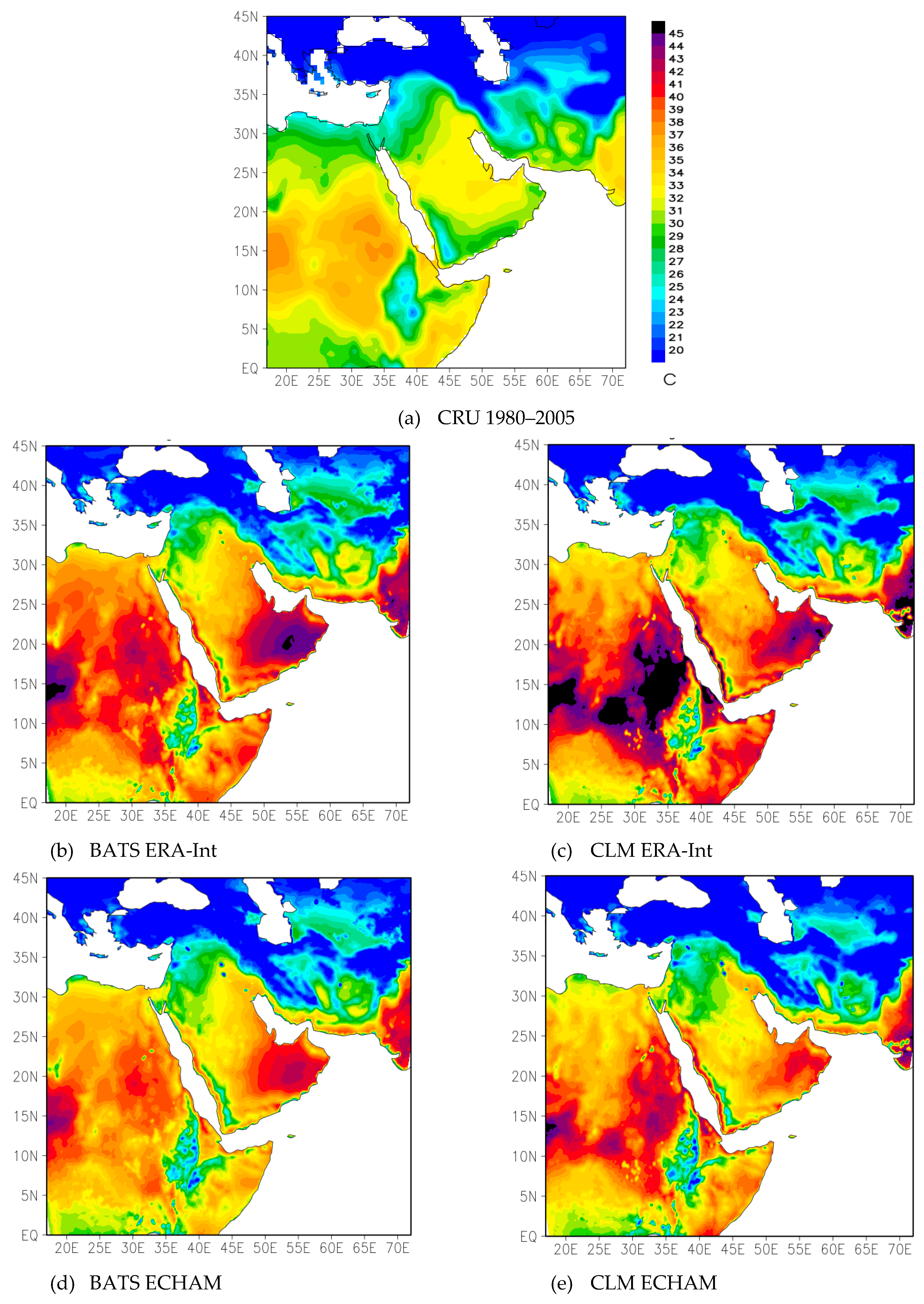
Figure 1. Spatial distribution of maximum temperature (°C) for (a) CRU, (b) ERA–Int BATS, (c) ERA–Int CLM, (d) ECHAM6 BATS, (e) ECHAM6 CLM, (f) GFDL BATS, (g) GFDL CLM, (h) HadGEM BATS, and (i) HadGEM CLM averaged over the period 1980–2005.
Atmosphere 10 00675 g001aAtmosphere 10 00675 g001b
Figure 2. Spatial distribution of minimum temperature (°C) for (a) CRU, (b) ERA–Int BATS, (c) ERA–Int CLM, (d) ECHAM6 BATS, (e) ECHAM6 CLM, (f) GFDL BATS, (g) GFDL CLM, (h) HadGEM BATS, and (i) HadGEM CLM averaged over the period 1980–2005.
Atmosphere 10 00675 g002aAtmosphere 10 00675 g002b
Figure 3. Spatial distribution of annual precipitation (mm) for (a) CRU, (b) ERA–Int BATS, (c) ERA–Int CLM, (d) ECHAM6 BATS, (e) ECHAM6 CLM, (f) GFDL BATS, (g) GFDL CLM, (h) HadGEM BATS, and (i) HadGEM CLM averaged over the period 1980–2005.
Atmosphere 10 00675 g003aAtmosphere 10 00675 g003b
Figure 4. Spatial distribution of annual warm days (TX90p) for (a) ERA–Int BATS, (b) ERA–Int CLM, (c) ECHAM6 BATS, (d) ECHAM6 CLM, (e) GFDL BATS, (f) GFDL CLM, (g) HadGEM BATS, and (h) HadGEM CLM averaged over the period 1986–2005 with reference period 1981–2000.
Atmosphere 10 00675 g004aAtmosphere 10 00675 g004b
Figure 5. Spatial distribution of annual warm nights (TN90p) for (a) ERA–Int BATS, (b) ERA–Int CLM, (c) ECHAM6 BATS, (d) ECHAM6 CLM, (e) GFDL BATS, (f) GFDL CLM, (g) HadGEM BATS, and (h) HadGEM CLM averaged over the period 1986–2005 with reference period 1981–2000.
Atmosphere 10 00675 g005aAtmosphere 10 00675 g005b
Figure 6. Spatial distribution of annual cold days (TX10p) for (a) ERA–Int BATS, (b) ERA–Int CLM, (c) ECHAM6 BATS, (d) ECHAM6 CLM, (e) GFDL BATS, (f) GFDL CLM, (g) HadGEM BATS, and (h) HadGEM CLM averaged over the period 1986–2005 with reference period 1981–2000.
Atmosphere 10 00675 g006aAtmosphere 10 00675 g006b
Figure 7. Spatial distribution of annual cold nights (TN10p) for (a) ERA–Int BATS, (b) ERA–Int CLM, (c) ECHAM6 BATS, (d) ECHAM6 CLM, (e) GFDL BATS, (f) GFDL CLM, (g) HadGEM BATS, and (h) HadGEM CLM averaged over the period 1986–2005 with reference period 1981–2000.
Atmosphere 10 00675 g007aAtmosphere 10 00675 g007b
Figure 8. Spatial distribution of annual warm spell duration index (WSDI) for (a) ERA–Int BATS, (b) ERA–Int CLM, (c) ECHAM6 BATS, (d) ECHAM6 CLM, (e) GFDL BATS, (f) GFDL CLM, (g) HadGEM BATS, and (h) HadGEM CLM averaged over the period 1986–2005 with reference period 1981–2000.
Atmosphere 10 00675 g008aAtmosphere 10 00675 g008b
Figure 9. Spatial distribution of annual cold spell duration index (CSDI) for (a) ERA–Int BATS, (b) ERA–Int CLM, (c) ECHAM6 BATS, (d) ECHAM6 CLM, (e) GFDL BATS, (f) GFDL CLM, (g) HadGEM BATS, and (h) HadGEM CLM averaged over the period 1986–2005 with reference period 1981–2000.
Atmosphere 10 00675 g009aAtmosphere 10 00675 g009b
Figure 10. Comparison of simulation based temperature indices (a) warm days, (b) warm nights, (c) cold days, (d) cold nights, (e) warm spell duration index, and (f) cold spell duration index, with the same obtained from observations for entire period of data available corresponding to each dataset.
Atmosphere 10 00675 g010
Figure 11. Spatial distribution of the number of annual wet days (R1mm) for (a) ERA–Int BATS, (b) ERA–Int CLM, (c) ECHAM6 BATS, (d) ECHAM6 CLM, (e) GFDL BATS, (f) GFDL CLM, (g) HadGEM BATS, and (h) HadGEM CLM averaged over the period 1986–2005.
Atmosphere 10 00675 g011aAtmosphere 10 00675 g011b
Figure 12. Spatial distribution of the annual number of annual consecutive wet days (CWD) for (a) ERA–Int BATS, (b) ERA–Int CLM, (c) ECHAM6 BATS, (d) ECHAM6 CLM, (e) GFDL BATS, (f) GFDL CLM, (g) HadGEM BATS, and (h) HadGEM CLM averaged over the period 1986–2005.
Atmosphere 10 00675 g012aAtmosphere 10 00675 g012b
Figure 13. Spatial distribution of the annual number of annual consecutive dry days (CDD) for (a) ERA–Int BATS, (b) ERA–Int CLM, (c) ECHAM6 BATS, (d) ECHAM6 CLM, (e) GFDL BATS, (f) GFDL CLM, (g) HadGEM BATS, and (h) HadGEM CLM averaged over the period 1986–2005.
Atmosphere 10 00675 g013aAtmosphere 10 00675 g013b
Figure 14. Comparison of simulation based precipitation indices (a) number of wet days, (b) consecutive wet days, and (c) consecutive dry days, with the same obtained from observations for the entire period of data available corresponding to each dataset.
Atmosphere 10 00675 g014aAtmosphere 10 00675 g014b
Figure 15. Spatial distribution of the wind vector (m/s) and relative humidity (%) for (a) ERA–Int BATS, (b) ERA–Int CLM, (c) ECHAM6 BATS, (d) ECHAM6 CLM, (e) GFDL BATS, (f) GFDL CLM, (g) HadGEM BATS, and (h) HadGEM CLM averaged over the period 1980–2005.
Atmosphere 10 00675 g015aAtmosphere 10 00675 g015b
Figure 16. Normal Quantile Plot for daily data of (a) maximum temperature (Tmax), (b) minimum temperature (Tmin), and (c) Precipitation for three CMIP5 models, reanalysis ERA-Int and surface observations for the period 1980–2005.
Atmosphere 10 00675 g016aAtmosphere 10 00675 g016b
Table 1. Observation based ETCCDI defined 27 climate extremes trends for the period 1978–2016.
Index Name Index LabelTrend/Decadep-Value
Summer dayssu2565.10.13
Max TXTXx5.70.13
Min TXTXn2.10.45
Max TNTNx7.20.07
Min TNTNn3.00.35
Cold daysTX10p−5.90.11
Warm daysTX90p18.00.03
Cold nightsTN10p−7.50.05
Warm nightsTN90p22.80.00
Warm spell durationWSDI75.80.06
Cold spell durationCSDI−18.10.22
Diurnal temperature rangeDTR−0.50.16
Max 1 day precipitationRX1day21.80.51
Max 5 day precipitationRX5day36.00.49
Simple day intensitySDII5.00.41
Heavy precipitation daysR10mm−2.00.40
Very heavy precipitation daysR20mm−0.10.45
Number of wet daysR1mm *−3.20.39
Consecutive wet daysCWD−0.40.52
Consecutive dry daysCDD−15.40.54
Very wet daysR95p40.30.44
Extremely wet daysR99p35.30.53
Total wet-day precipitationPRCPTOT−18.90.46
Note: If the p-value less than or equal to the significance level α = 0.05, the null hypothesis is rejected and the significance is at the 95% confidence level. The * symbol with R1mm indicates the user defined threshold which is 1mm for this study.
Table 2. Comparison of simulation-based trends with the same obtained from the observations for the common period 1980–2005.
ERA-BATSERA-CLMGFDL-BATSGFDL-CLMHadGEM-BATSHadGEM-CLMECHAM-BATSECHAM-CLMAll-BATSAll-CLMAll-ModelsObserved
TX90p−1.2−2.55.9c6.4c10.0c7.9c5.4a4.6a5.1c4.1c4.6c32.3c
TN90p3.93.210.0c8.0c12.3c11.6c9.0c9.8c8.8c8.2c8.5c12.1c
TX10p−2.2−2.2−3.7−0.3−2.6−3.7a−3.5−1.3−3.0b−1.9−2.5−9.6c
TN10p−3.1−5.6a−5.8a−4.9a−3.4−3.8a−6.4b−6.6b−4.7c−5.2c−5.0c−7.7c
WSDI0.1−0.21.3c1.2c2.5c1.7c1.10.9a1.2c0.9c1.1c5.6c
CSDI−0.9−1.2−1.9b−1.7b−0.9−0.9−1.5b−1.6b−1.3c−1.4c−1.3c−1.6c
R1mm1.1−0.10.62.01.3−0.32.12.11.30.91.1−0.3
CDD−0.5−0.9−1.1−7.4−5.7a−5.4a−9.4a−9.4a−4.2−5.8b−5.0a−12.2
CWD0.7−0.11.01.21.1−0.10.50.90.80.50.70.1
Note: The superscript a, b and c represents a significant level 90%, 95%, and 99% respectively.