GNSS Ionosphere Sounding of Equatorial Plasma Bubbles

Abstract

Ground- and space-based Global Navigation Satellite System (GNSS) receivers can provide three-dimensional (3D) information about the occurrence of equatorial plasma bubbles (EPBs). For this study, we selected March 2014 data (during solar maximum of cycle 24) for the analysis. The timing and the latitudinal dependence of the EPBs occurrence rate are derived by means of the rate of the total electron content (TEC) index (ROTI) data from GNSS receivers in China, whereas vertical profiles of the scintillation index S4 are provided by COSMIC (Constellation Observing System for Meteorology, Ionosphere and Climate). The GNSS receivers of the low Earth orbit satellites give information about the occurrence of amplitude scintillations in limb sounding geometry where the focus is on magnetic latitudes from 20° S to 20° N. The occurrence rates of the observed EPB-induced scintillations are generally smaller than those of the EPB-induced ROTI variations. The timing and the latitude dependence of the EPBs occurrence rate agree between the ground-based and spaceborne GNSS data. We find that EPBs occur at 19:00 LT and they are mainly situated above the F2 peak layer which descended from 450 km at 20:00 LT to 300 km at 24:00 LT in the equatorial ionosphere. At the same time, the spaceborne GNSS data also show, for the first time, a high occurrence rate of post-sunset scintillations at 100 km altitude, indicating the coexistence of equatorial sporadic E with EPBs.

1. Introduction

Manifested as irregular electron density or total electron content (TEC) variations, the equatorial plasma bubbles (EPBs) are a phenomenon related to the collisional Rayleigh-Taylor instability (RTI) mechanisms. Although the onset condition remains unclear, the RTI is believed to occur after sunset at low latitudes near magnetic equator and generates plasma depletions which grow up from the bottom side to the upper F layer. While moving upward, EPBs extend along the magnetic flux tube to higher latitudes and often reach the equatorial ionization anomaly crest [1]. These plasma irregularities disturb radio communication and navigation by causing phase and amplitude scintillations or even signal loss, which is an important issue for space weather [2]. Furthermore, the study of the RTI and EPBs is relevant to progress in understanding and modeling of ionospheric plasma physics.

The study of EPBs has gone a long way since it was first recorded as equatorial spread F (ESF) with ionosonde [3]. The term EPBs was proposed when ground-based incoherent scatter radar detected low-density irregularities rising from the bottom side of F layer to an altitude far beyond the ionospheric peak [4]. These irregularities were directly confirmed by AE-C satellite in-situ measurements to be regions with an abrupt decrease of electron density by two orders of magnitude with tens of kilometers scale [5]. The optical imaging techniques probed a two-dimensional structure of the plasma bubble [6]. Effects of scintillations on radio waves from the stars or satellites have been also used to investigate the behavior of EPBs. TEC fluctuation measured with ground-based Global Navigation Satellite System (GNSS) networks can capture occurrence and evolution of EPBs and reveal their longitudinal occurrence characteristics as well [2,7]. Spaceborne GNSS radio occultation of Constellation Observing System for Meteorology, Ionosphere, and Climate (COSMIC) complements the ground-based observations of EPBs with its global coverage. Moreover, it is crucial to obtain the vertical structure of the ionosphere [8]. For this reason, basing on GNSS and radio occultation measurements, a three-dimensional morphology of EPBs was deduced and a tomography method was attempted to reconstruct EPBs in a Brazilian sector [9,10].

Recent researches on RTI and EPBs have been driven mostly by space weather concerns to identify the key environmental parameters leading to the presence of EPBs. Comprehensive observation can reveal the structure and evolution of EPBs that are connected with their initial conditions. This paper aims to investigate the characteristics of EPBs in space- and ground-based GNSS data. The scintillation index S4 and electron density of the ionosphere, profiled by spaceborne GNSS radio occultation of COSMIC, can provide new information on their vertical structure, occurrence, and evolution process of EPBs. Together with ground-based observation, three-dimensional aspects of EPBs can be inspected. We focus on low latitude regions at longitude ~110° E in south China in March 2014 when EPBs occurred every day of the month, and therefore a common underlying cause to seed the RTI can be examined. We use GNSS radio occultation of COSMIC to derive the vertical structure of EPBs and relate their characteristics with ground-based GNSS measurements in China. Global distribution of irregularities occurrence is also presented. Section 2 introduces data and analysis methods. Our results are described in Section 3, where TEC fluctuation and occurrence from ground-based GNSS observation are displayed in Section 3.1, as well as temporal variations of electron density and EPBs occurrence profiles, global occurrence of scintillations caused by EPBs, and sporadic E (E_s) from COSMIC are shown in Section 3.2. Section 4 presents a discussion of a comprehensive view of EPBs by combining both ground-based and space-based observations and referencing previous research findings. The conclusions are drawn in Section 5.

2. Data and Methods

Ground-based GNSS observations are provided by the Crustal Movement Observation Network of China (CMONOC). Eighteen GNSS receivers are selected to form a chain-like configuration along 110° E of longitude, covering a range in latitude between 16.8° N and 35.1° N (corresponding to a magnetic latitude between 7.0° N and 25.2° N), as shown in Figure 1.

With a thin layer ionosphere model at 400 km, the tracks of the ionospheric piercing point (IPP) have latitude coverage from ~12° N to ~40° N. The slant total electron content (TEC) was calculated with carrier phase measurement performed every 30 s for each receiver. To mitigate multipath effects, only data with satellite elevation larger than 30 degrees was used. The rate of change of TEC (ROT) was determined by taking the difference between the slant TECs at two consecutive times. Calculated on a 5 min time window with 11 successive measurements, the rate of TEC index (ROTI) is defined as the standard deviation of ROT and it is used to quantify TEC fluctuation in time and space [7]. An irregularity encounter is reckoned if more than 20 consecutive ROTIs are larger than a threshold, which is around 0.2 TECU/min; this threshold, that could be different for different receivers, is described as the sum of the average plus 10 times root mean square (RMS) of all ROTIs collected during daytime 6:00 LT to 18:00 LT for a receiver. In this study, to show vertical TEC fluctuation, we use the vROTI, which can be converted from ROTI, analogously as TEC can be converted from slant TEC. An image of vROTI in latitudinal-temporal variation is obtained by binning vROTI into 0.3° × 30 min latitude-local time grid cells. Occurrence of irregularities is defined by the ratio of ROTI larger than the threshold to all ROTI recorded within the grid cell.

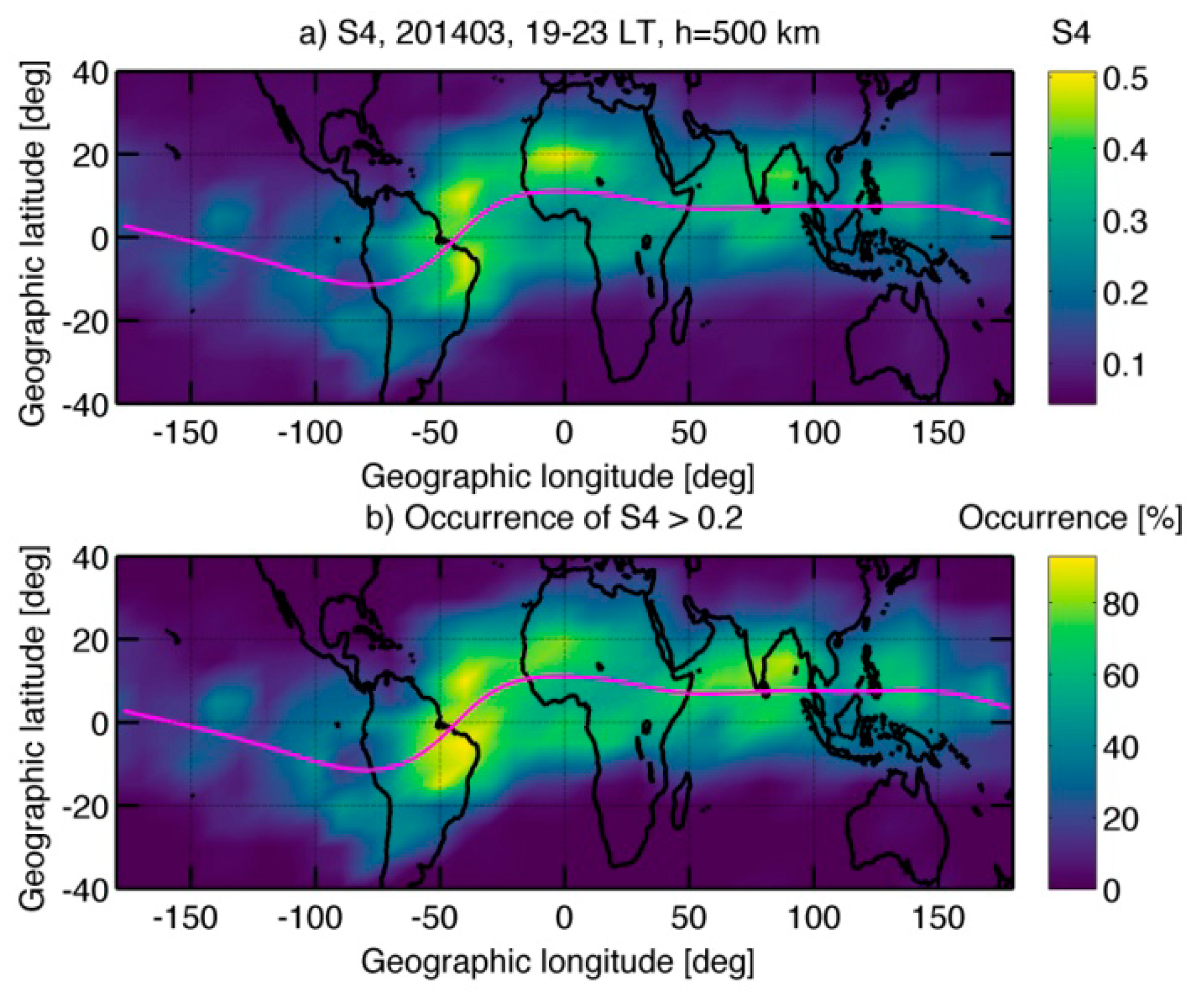
The space-based observations we used are electron density (N_e) and scintillation index S4 from COSMIC radio occultation of GNSS. Defined by the normalized RMS of GPS L1 signal intensity fluctuation, S4 is derived from the 50 Hz measurements of L1 amplitude and the output of the S4 profiles is in 1 Hz sampling rate. A large electron density fluctuation tends to cause a large signal intensity fluctuation. S4 > 0.2 is taken as a threshold to identify the ionospheric irregularities. The mean of N_e profiles at different time is obtained by binning the N_e data into 10 km × 1 h grid cell and taking the arithmetic average within ±20° magnetic latitudes. The vertical profiles of S4 in the altitude range of 90–710 km are used to display height variations of irregularities. To examine the global distribution of S4 at different heights, the data was binned into 5° × 10° latitude-longitude grid cells and occurrence of irregularities is defined by the ratio of samples with S4 > 0.2 to all S4 measured within the grid cell.

The ionosphere at low latitude can be related to that at the magnetic equator by magnetic lines. On the basis of the International Geomagnetic Reference Field (IGRF), Figure 2 shows a sketch of magnetic lines at the longitude of 110° E which can relate the apex height at the magnetic equator (7° N) to the latitudinal coordinate. The magnetic line crossing the ionosphere (at 400 km) at 23° N has an apex height of ~1000 km at the magnetic equator, while the magnetic line crossing the ionosphere at 30° N has an apex height of ~1500 km at the magnetic equator.

3. Results

3.1. vROTI at ~110° E in China in March 2014

Plasma bubbles occur in low-latitude regions near the magnetic equator. Their extension along the magnetic flux tube to higher latitudes was observed by the meridional chain of GNSS receivers. By surveying the whole year data of 2014, we found that irregularities in latitudes lower than 22° N showed maximum occurrence in equinoxes, those in latitudes larger than 22° N showed different behaviors. We focus on March when ionospheric irregularities were detected every day by three GNSS receivers between 16° N and 20° N, so that common characteristics can be investigated. Figure 3 displays temporal variation of vROTI, selected from observations of five GNSS receivers from 16.8° N to 30.3° N at ~110° E in March 2014. Although the latitude and longitude differences are 3.2° and 2.1°, respectively between Yong and Hihk, both receivers observed ionospheric irregularities, with comparable magnitudes, that occurred at ~19:00 LT every day. The magnitude of vROTI is also comparable between the two receivers. From Hihk to other stations, the monthly occurrence rate decreases with latitude, and also does vROTI. At Hbes (latitude 30.3° N), weak irregularities were observed within a short time for several days.

By binning vROTI and all Roti values into 0.3° × 30 min latitude-local time grid cells, the mean vROTI and occurrence for ROTI larger than the threshold were calculated for each grid cell. Figure 4 shows the temporal and latitudinal variations of mean vROTI (color) and occurrence contour (white line) for the EPB-induced irregularities, respectively. With the appearing of EPBs at ~19:00 LT, vROTI increased very quickly with time, between 12° N and 19° N. From ~20:00 LT to ~23:00 LT, vROTI was generally large and fluctuated around 1.0 TECU/min, while EPBs had high occurrence (65% to 90%). The strongest of vROTI was seen at ~20/21:00 LT around 16° N. The largest occurrence was seen around 13° N at ~22:00 LT. From ~23:00 LT, vROTI and EPB-induced occurrence decreased with time until ~2:00 LT after midnight. From 19° N to 30° N, vROTI was smaller than 1 TECU/min, and the time of occurrence was delayed with latitude. Compared with those in lower latitudes, EPBs existed for a shorter time and the occurrence rate decreased with latitude. At latitudes larger than 28° N, the 10% occurrence appeared after 22:00 LT and disappeared before midnight.

3.2. EPBs Observed by COSMIC

The vertical structures of EPBs, as shown in Figure 5, are obtained by binning the N_e and S4 data into 10 km × 1 h and taking the arithmetic average of N_e and percentage of S4 > 0.2 within ±20° magnetic latitudes. The image shows the background ionosphere in vertical and temporal dimensions. The maximum electron density, denoted by yellow color, represents F peak ionosphere. At ~17:00 LT the bottom side of F peak went up from ~300 km to ~390 km at ~18:30 LT. From ~18:30 LT to ~20:00 LT the F peak was located at ~390–530 km. From ~20:00 LT the ionosphere declined linearly with time until midnight and remained at about 250–320 km after midnight. While the F layer was declining, the electron density of F peak maintained a level of 1.5 × 10⁶/cm⁻³ until ~23:00 LT. Then it decreased to ~6 × 10⁵/cm⁻³ until ~2:00 LT and maintained such low level thereafter. The electron density is very low below the F layer.

The white contour lines show the EPB-induced occurrence of S4 > 0.2 which is an indicator of the existence of EPBs. Centering at the top side of F peak, EPBs started to appear at ~19:00 LT and occupied a height range between 380 km and 650 km. The occurrence rapidly increased with time to 30–40% at ~20:00 LT for an altitude ranging from 400 km to 650 km, the 20% occurrence line reached 700 km at the same time. The largest occurrence of 50% was registered at ~21:00 LT from ~450 km to ~510 km; below 400 km there are time delays to reach the largest occurrence as compared with those at altitudes above 400 km. The occurrence increased at lower speed and reached the largest after ~22:00 LT, and the lower the altitude the later the occurrence reached its largest. The smallest gradient aligned with the declination of the F layer. In two-dimensional view, the orientation of the contours aligned with the orientation of the maximum electron density. The altitude of the higher bound of 20% contour decreased with time to the altitude of about 250–300 km after midnight. For the altitude of 150–220 km, the occurrence of 20% appeared after 20:00 LT and reached the largest at midnight. Then, it decreased with time until ~2:00–2:30 LT.

It should be pointed out that the occurrence of S4 > 0.2 also happened at lower altitude between 100 km and 130 km which can be related with sporadic E (E_s). At 100 km, the 20% occurrence appeared at ~18:40 LT, which is 20 min earlier than that of EPBs. Then, it rapidly increased with time, reached the largest of 55% at 22 LT and, then, it decreased less rapidly with a 20% occurrence ending at ~2:30 LT. Moreover, the occurrence delayed with altitude; in fact, away from 100 km, the occurrence varied slowly with time.

Figure 6 shows the dependence of the occurrence rate of S4 > 0.2 on the magnetic latitude and height (all longitudes are included). It is evident that the scintillations either occurred at low latitudes or at high latitudes. The scintillations of COSMIC disappeared at magnetic middle latitudes from 30° to 60° which was similar to the ground-based GNSS observations in China. It is worth noticing the connection between EPBs and sporadic E, at 10° S to 0° S. While EPBs were maximal at 400 km altitude and higher, the polar scintillations mainly occurred at 250–400 km altitude.

The global distribution of S4 was investigated to understand the longitudinal characteristics of EPBs occurrence. As shown in Figure 7, the EPBs at 500 km were studied with latitude ranging from 40° S to 40° N. The magenta line in every panel represents the magnetic equator. Although not symmetric about the magnetic equator in strength and occurrence, scintillations happened mainly within ±15° magnetic latitudes. The scintillation in northern anomaly is generally stronger than that in southern anomaly, as shown in Figure 7a. Three areas of maximum S4 (equal to 0.5) can be seen at Atlantic, Africa, and Asia. Figure 7b shows that the global distribution of EPBs occurrence has a similar pattern to S4; this occurrence, in fact, can be as large as 80% over Atlantic, Africa, and Asia. On the contrary, EPBs were weaker and their occurrence was less frequent over the Pacific.

Similar to that of Figure 7 and Figure 8 displays the global distribution of S4 and occurrence of E_s at 100 km with latitude ranging from 50° S to 50° N. Aligning with the magnetic equator, larger S4 is observed from 25° S to 40° N for the longitude range of 100° W–150° E, as revealed in Figure 8a. Over America, it ranges from 50° S to 25° N. Three belts can be distinguished at 20° S, 0, and 20° N in magnetic latitude, respectively. There are also three active areas over the Atlantic, Africa, and Asia, similar to S4 at 500 km in Figure 7. Moreover, the maximum of S4 generally occurred at the magnetic equator and reached the largest value of one. As to the characteristics of E_s occurrence, Figure 8b shows that its latitude and longitude dependences are similar to those of S4. It can reach a value of 100% and it is generally larger at the magnetic equator than at low latitudes, however, the pattern of three belts is not so obvious in occurrence distribution. Similar to the previous case (500 km), E_s was weaker, and its occurrence was less frequent over the Pacific.

4. Discussion

It is understood that the pre-reversal eastward electric field enhancement (PRE) near sunset uplifts the F layer and contributes to the growth rate of the generalized RTI which is responsible for EPBs. During March 2014, EPBs occurred every day up to the latitude of 20° N at ~110° E longitude, as shown in Figure 3. It is well known that the occurrence of EPBs tends to peak at equinoxes especially at high solar activity. The year 2014 was a year of maximum activity of solar cycle 24, even though the geomagnetic activity was generally low in March (the largest −Dst was 52 nT on March 1 and the largest K-index was 4 on March 25). Under magnetically quiet conditions, higher solar activity implies greater pre-reversal eastward electric field, as well as earlier occurrence and earlier decay of EPBs [11,12]. Nishioka et al. reported a 70% occurrence rate in the Asian region in previous solar maximum 2002 (a year during maximum phase of solar cycle 23) when the solar radio flux F10.7 had a similar level to that of 2014 [13]. Such a 100% monthly occurrence rate of EPBs is very special.

The monthly mean vROTI and EPB-induced occurrence in the 0.3° × 30 min latitude-local time map in Figure 4 showed average properties of EBPs in March 2014. In the latitude range between 12° N and 19° N, EPBs started to appear at ~19:00 LT. vROTI had high value from ~20:00 LT to ~23:00 LT. The strongest value was observed at ~20:00–21:00 LT around 16° N; while the largest occurrence (90%) was observed around 13° N at ~22:00 LT. From ~23:00 LT, vROTI decreased with time until EPBs disappeared at ~2:00 LT after midnight. From 19° N to 30° N, the occurrence of the irregularities delayed with latitude and existed for a shorter time with increasing latitude. The highest latitude of 10% occurrence reached ~28° N. Referencing Figure 2, the magnetic field line at 400 km at ~19–28° N has an apex height of ~750–1000 km at the magnetic equator. This suggests that every day near the magnetic equator EPBs reached the altitude of 750 km about 1 h after their occurrence and some days came to the altitude of 1000 km.

The space-based GNSS observations agreed well with the ground-based ones. The vertical structure of the ionosphere background and the occurrence of EPBs at magnetic equator in Figure 5 showed that after sunset, the occurrence and development of EPBs is accompanied by the uplift of the F layer, giving direct evidence of eastward electric field. EPBs mainly occurred at and above the F peak. The observed S4 scintillation occurrence was generally smaller than those shown by ROTI. The timing and the latitude dependence of the EPBs occurrence rate agreed between the ground-based and space-based GNSS data, however, the evolution of the EPBs seen from ground-based and space-based GNSS receivers was different. Together with the declining of EPBs, the F peak declined from 450 km at 20:00 LT to 300 km at 24:00 LT in the equatorial ionosphere as seen by COSMIC in Figure 5. This can be attributed to the strong post-reversal westward background electric field in high solar activity [11,12]. As GNSS observation reflects line integral effects, the height variation of the irregularities would not change vROTI much. There is no declination of vROTI occurrence at ~20:00 LT in Figure 4, actually the occurrence for 17–28° N continued to increase after 20:00 LT. The occurrence from 12° N to 19° N started to decrease at ~21:00–22:00 LT and for higher latitudes it started to decrease after midnight. The irregularities in latitudes lower than ~19° N persisted longer than those in latitudes larger than ~19° N.

Furthermore, the spaceborne GNSS also detected scintillation at 100 km to 130 km which indicates the existence of E_s layer at low magnetic latitudes. Looking at lower heights in Figure 5, it appears that E_s occurred about 20 min earlier than EPBs. E_s occurrence increased with time and reached the largest at ~22:00 LT, 1 h later than EPBs. They disappeared after midnight at about the same time as that of EPBs. Although there are many researches on low to mid latitudes E_s and their interaction with bottom side of F layer to seed RTI [14], the nighttime E_s at magnetic equator has not often been reported, especially the E_s appeared in the evening and continued to post midnight. Actually, E_s near magnetic equator could be disrupted while the F layer was uplifted to higher altitude, which is associated with competing conditions of zonal wind shear and upward vertical electric field [15]. With data of COSMIC for 2006 to 2011, E_s was very rare in the magnetic equatorial zone. Model simulation showed E_s layer occurrences in low-latitude and equatorial regions do not correlate well with the zonal wind shear [16]. The downward vertical electric field resulted from post-reversal westward electric field probably play a role in the E_s formation at the magnetic equator, however, this cannot explain the earlier occurrence of E_s in the evening.

The global distribution of EPBs was confined to equatorial ionization anomaly regions as shown in Figure 7. Strongest scintillation occurred at magnetic equator and both equatorial ionization anomaly regions, as reported in previous studies [1]. EPBs were stronger and had higher occurrence over Atlantic, Africa, and Asia. This is in agreement with the result derived from global ground-based GPS receiver networks [13]. The longitudinal distribution of E_s was similar to that of EPBs. However, E_s distributed in a larger latitudinal range of ±20° magnetic latitudes, and it was stronger at magnetic equator and ~20° away from the magnetic equator. The magnetic field line at ~100 km at 20° magnetic latitude had an apex height of ~400 km, excluding the possibility of this latitude E_s for seeding EPBs.

Although the mechanisms for seeding EPBs and producing E_s are different, their correlation of occurrence in time implies coupling between the E and F layers, and a common factor probably underlies the formation of both irregularities. Gravity wave seeding from below might be a cause for generation of E_s and EPBs in the equatorial post-sunset ionosphere [17,18]. In addition, there is a decrease of both EPBs and sporadic E in the equatorial post-sunset ionosphere over the Pacific. These features suggest a connection between EPBs and sporadic E, at the magnetic equator.

5. Conclusions

Characteristics of EPBs in March 2014 were investigated with ground-based and space-based GNSS observations. GNSS receivers at ~110° E in the latitude range of 16.8° N to 35.1° N found EPBs every day up to 20° N. Accompanied by the uplift of F layer EPBs appeared at ~19:00 LT and reached altitude ~750 km within ~1 h. The occurrence of the EPB-induced scintillations was generally smaller than those of the EPB-induced ROTI variations. The timing and the latitude dependence of the EPBs occurrence rate agree between the ground-based and space-based GNSS data. EPBs mainly situated above the F peak which descended from 450 km at 20:00 LT to 300 km at 24:00 LT in the equatorial ionosphere. The EPB-induced irregularities persisted longer in lower latitudes than those over the magnetic equator. The spaceborne GNSS also detected E_s at 100 km altitude mainly at the magnetic equator and ±20° magnetic latitudes. They occurred a little earlier than the EPBs and disappeared at the same time as the EPBs above the magnetic equator. The occurrence of both EPBs and E_s decreased in the equatorial post-sunset ionosphere over the Pacific.

While the result on the vertical structure and temporal variation of EPBs is consistent with previous work, the longer persistence of EPB-induced irregularities in lower latitudes is reported for the first time. The nighttime E_s at the magnetic equator and its coexistence with EPBs are new findings. There is probably a connection between EPBs and E_s at the magnetic equator which is interesting for future observations and simulations.

References

1. Balan, N.; Liu, L.B.; Le, H.J. A brief review of equatorial ionization anomaly and ionospheric irregularities. Earth Planet. Phys. 2018, 2, 257–275. [Google Scholar] [CrossRef]
2. Kintner, P.M.; Ledvina, B.M.; De Paula, E.R. GPS and ionospheric scintillations. Space Weather 2007, 5, S09003. [Google Scholar] [CrossRef]
3. Booker, H.G.; Wells, H.W. Scattering of radio waves by the F-region of the ionosphere. J. Geophys. Res. Space Phys. 1938, 43, 249–256. [Google Scholar] [CrossRef]
4. Woodman, R.F.; La Hoz, C. Radar observations of F region equatorial irregularities. J. Geophys. Res. Space Phys. 1976, 81, 5447–5466. [Google Scholar] [CrossRef]
5. McClure, J.P.; Hanson, W.B.; Hoffman, J.H. Plasma bubbles and irregularities in the equatorial ionosphere. J. Geophys. Res. Space Phys. 1977, 82, 2650–2656. [Google Scholar] [CrossRef]
6. Weber, E.J.; Buchau, J.; Eather, R.H.; Mende, S.B. North-south aligned equatorial airglow depletions. J. Geophys. Res. Space Phys. 1978, 83, 712. [Google Scholar] [CrossRef]
7. Pi, X.; Mannucci, A.J.; Lindqwister, U.J.; Ho, C.M. Monitoring of global ionospheric irregularities using the worldwide GPS network. Geophys. Res. Lett. 1997, 24, 2283–2286. [Google Scholar] [CrossRef]
8. Watson, C.; Pedatella, N.M. Climatology and Characteristics of Medium-Scale F Region Ionospheric Plasma Irregularities Observed by COSMIC Radio Occultation Receivers. J. Geophys. Res. Space Phys. 2018, 123, 8610–8630. [Google Scholar] [CrossRef]
9. Park, J.; Lühr, H.; Noja, M. Three-dimensional morphology of equatorial plasma bubbles deduced from measurements onboard CHAMP. Ann. Geophys. 2015, 33, 129–135. [Google Scholar] [CrossRef] [Green Version]
10. Prol, F.; Hernandez, M.; Honorato, M.; Camargo, P. Tomographic imaging of ionospheric plasma bubbles based on GNSS and radio occultation measurements. Remote. Sens. 2018, 10, 1529. [Google Scholar] [CrossRef]
11. Hysell, D.; Burcham, J. Long term studies of equatorial spread F using the JULIA radar at Jicamarca. J. Atmos. Solar-Terr. Phys. 2002, 64, 1531–1543. [Google Scholar] [CrossRef]
12. Fejer, B.G.; Scherliess, L.; De Paula, E.R. Effects of the vertical plasma drift velocity on the generation and evolution of equatorial spread F. J. Geophys. Res. Space Phys. 1999, 104, 19859–19869. [Google Scholar] [CrossRef]
13. Nishioka, M.; Saito, A.; Tsugawa, T. Occurrence characteristics of plasma bubble derived from global ground-based GPS receiver networks. J. Geophys. Res. Space Phys. 2008, 113, A05301. [Google Scholar] [CrossRef]
14. Tsunoda, R.T. Seeding of equatorial plasma bubbles with electric fields from an Es-layer instability. J. Geophys. Res. Space Phys. 2007, 112, A06304. [Google Scholar] [CrossRef]
15. Abdu, M.A.; MacDougall, J.W.; Batista, I.S.; Sobral, J.H.A.; Jayachandran, P.T. Equatorial evening prereversal electric field enhancement and sporadic E layer disruption: A manifestation of E and F region coupling. J. Geophys. Res. Space Phys. 2003, 108, 1254. [Google Scholar] [CrossRef]
16. Chu, Y.H.; Wang, C.Y.; Wu, K.H.; Chen, K.T.; Tzeng, K.J.; Su, C.L.; Feng, W.; Plane, J.M.C. Morphology of sporadic E layer retrieved from COSMIC GPS radio occultation measurements: Wind shear theory examination. J. Geophys. Res. Space Phys. 2014, 119, 2117–2136. [Google Scholar] [CrossRef]
17. Hocke, K.; Tsuda, T. Gravity waves and ionospheric irregularities over tropical convection zones observed by GPS/MET Radio Occultation. Geophys. Res. Lett. 2001, 28, 2815–2818. [Google Scholar] [CrossRef] [Green Version]
18. Krall, J.; Huba, J.D.; Fritts, D.C. On the seeding of equatorial spread F by gravity waves. Geophys. Res. Lett. 2013, 40, 661–664. [Google Scholar] [CrossRef]
Figure 1. Geographical location of all 18 GNSS receivers (described in the text) in the 100° E to 120° E and 10° N to 40° N sector.
Atmosphere 10 00676 g001
Figure 2. A sketch of magnetic lines from the magnetic equator to low latitudes.
Atmosphere 10 00676 g002
Figure 3. vROTI variations with time in March 2014.
Atmosphere 10 00676 g003
Figure 4. Mean vROTI (color) and occurrence of EPBs (ROTI > threshold, white contour lines) in local time and latitude.
Atmosphere 10 00676 g004
Figure 5. The variation of background ionosphere (color) and the occurrence of EPBs (scintillation index S4 > 0.2, white contour lines) observed by COSMIC in March 2014 and averaged for the interval from 20° S to 20° N magnetic latitude.
Atmosphere 10 00676 g005
Figure 6. Occurrence rate of S4 > 0.2 as a function of magnetic latitude and height for local times from 19:00 to 23:00 LT observed by COSMIC in March 2014.
Atmosphere 10 00676 g006
Figure 7. Global distribution of (a) S4 and (b) the occurrence of S4 > 0.2 at 500 km observed by COSMIC in March 2014. Magnetic equator is represented by a magenta line in every panel.
Atmosphere 10 00676 g007
Figure 8. Global distribution of (a) S4 and (b) the occurrence of S4 > 0.2 at 100 km observed by COSMIC in March 2014.
Atmosphere 10 00676 g008