Impacts of the Desiccated Lake System on Precipitation in the Basin of Mexico City

 , , , and
Abstract
:1. Introduction
2. Methods
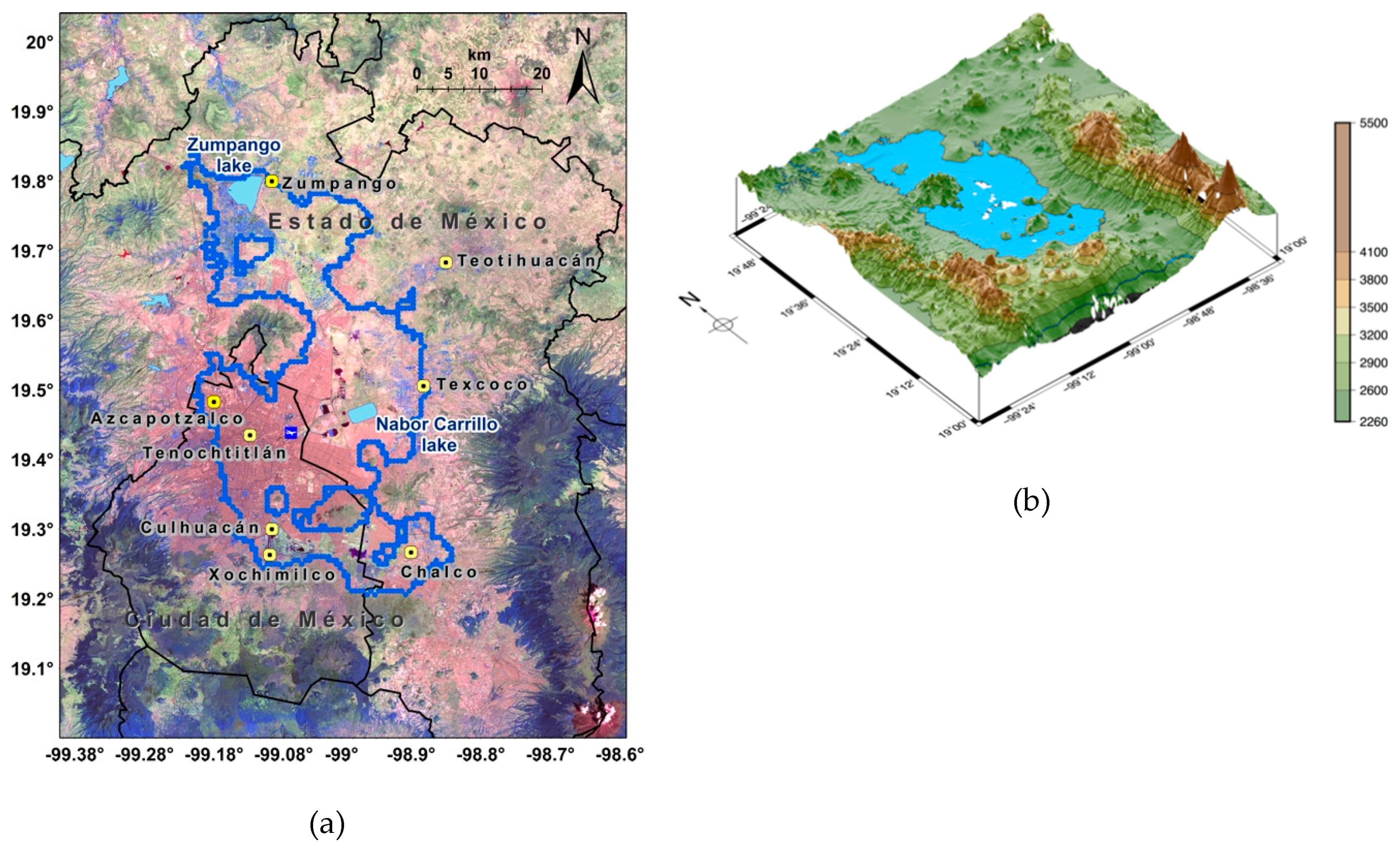
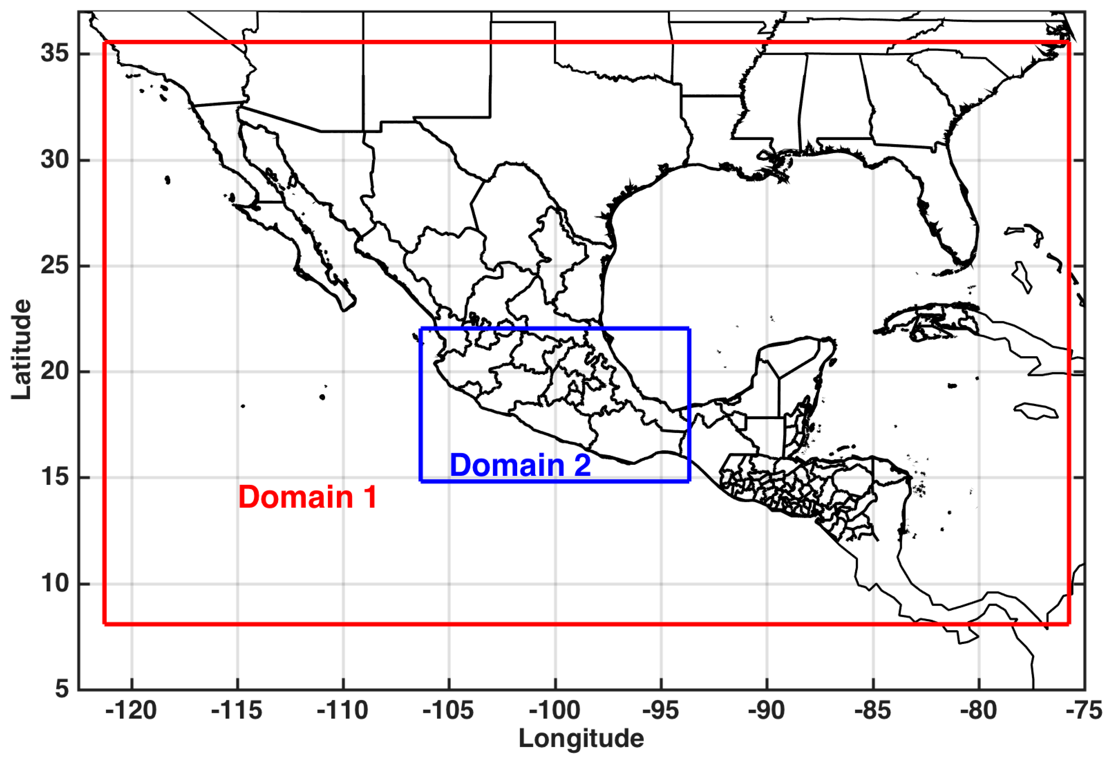
2.1. Study Area
2.2. WRF Model Configuration
3. Results
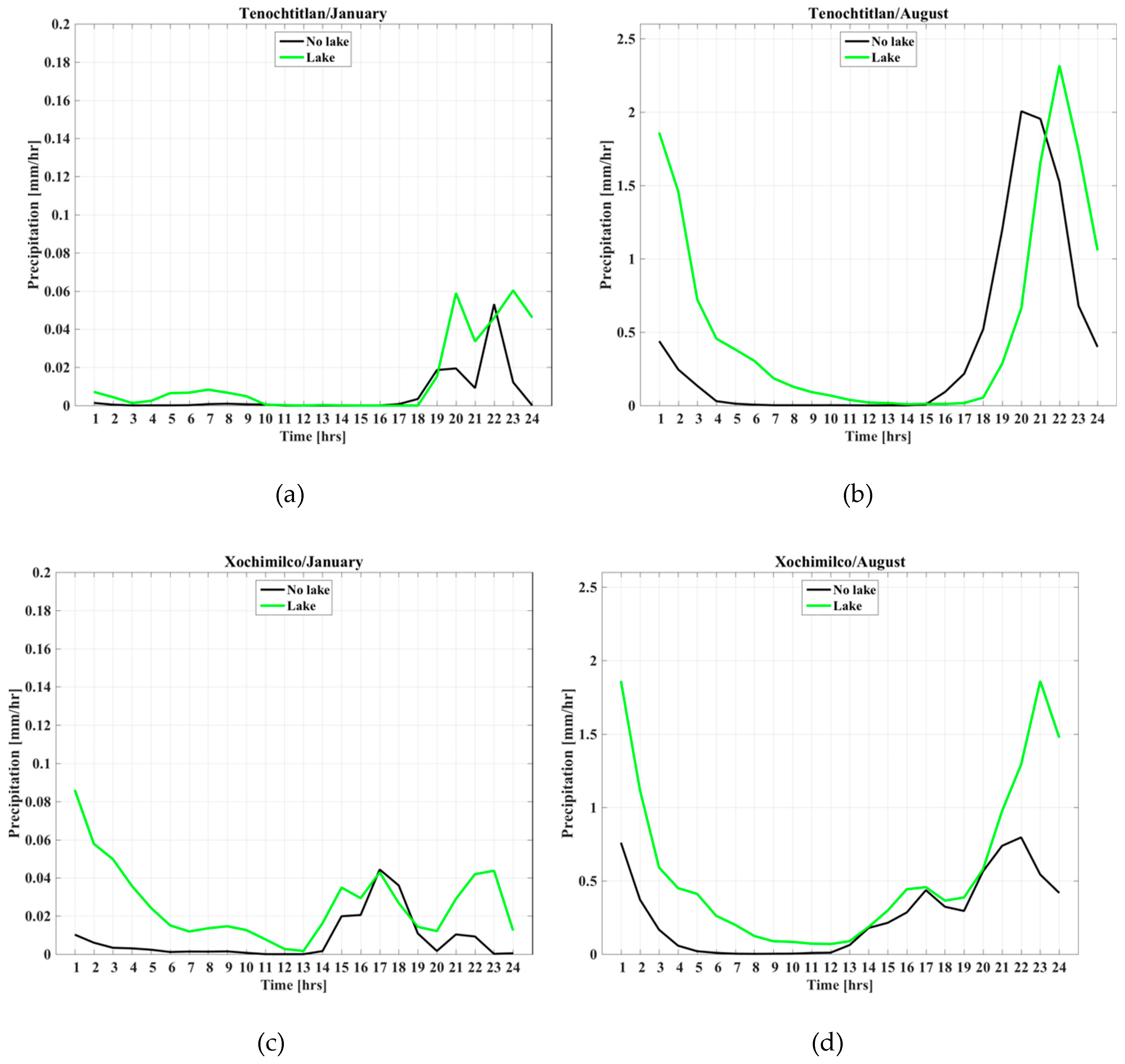
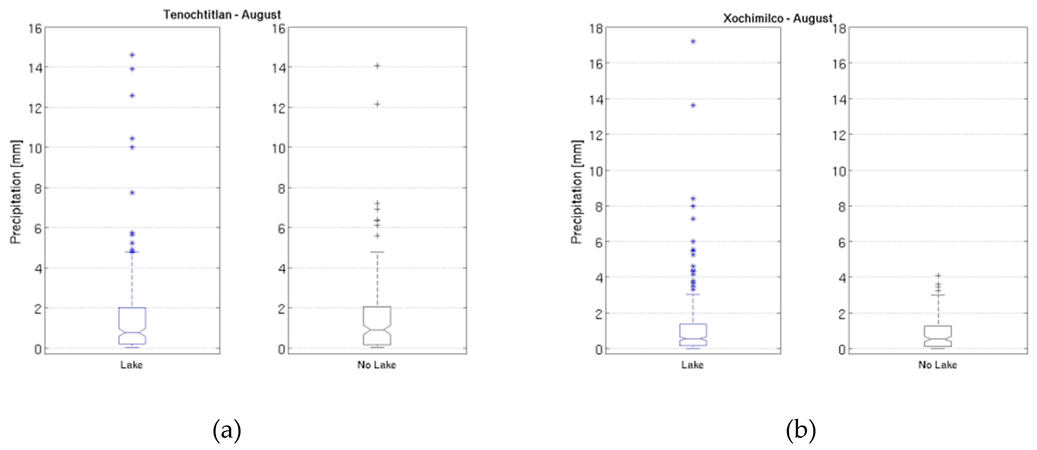
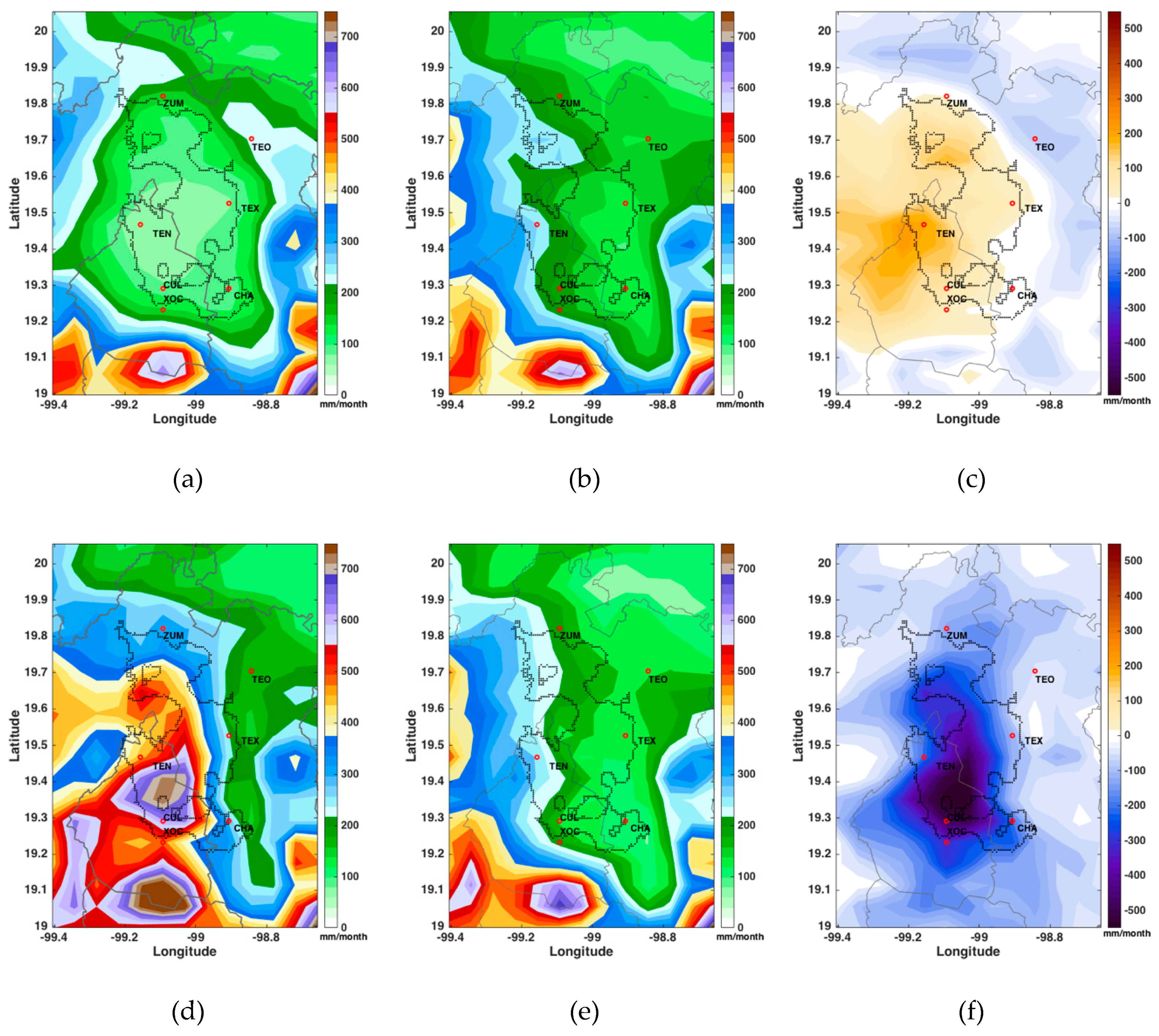
3.1. Precipitation
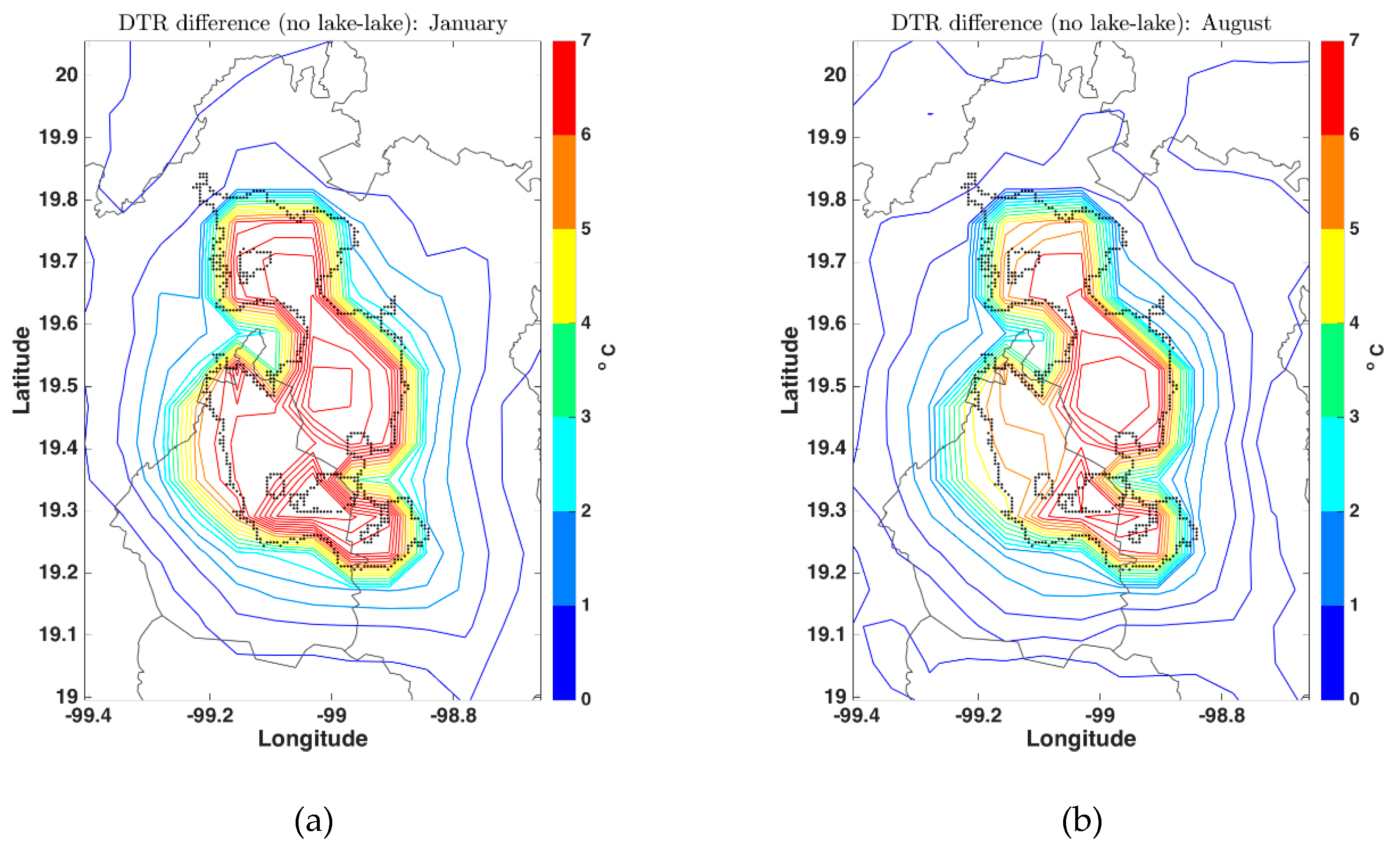
3.2. Air Temperature
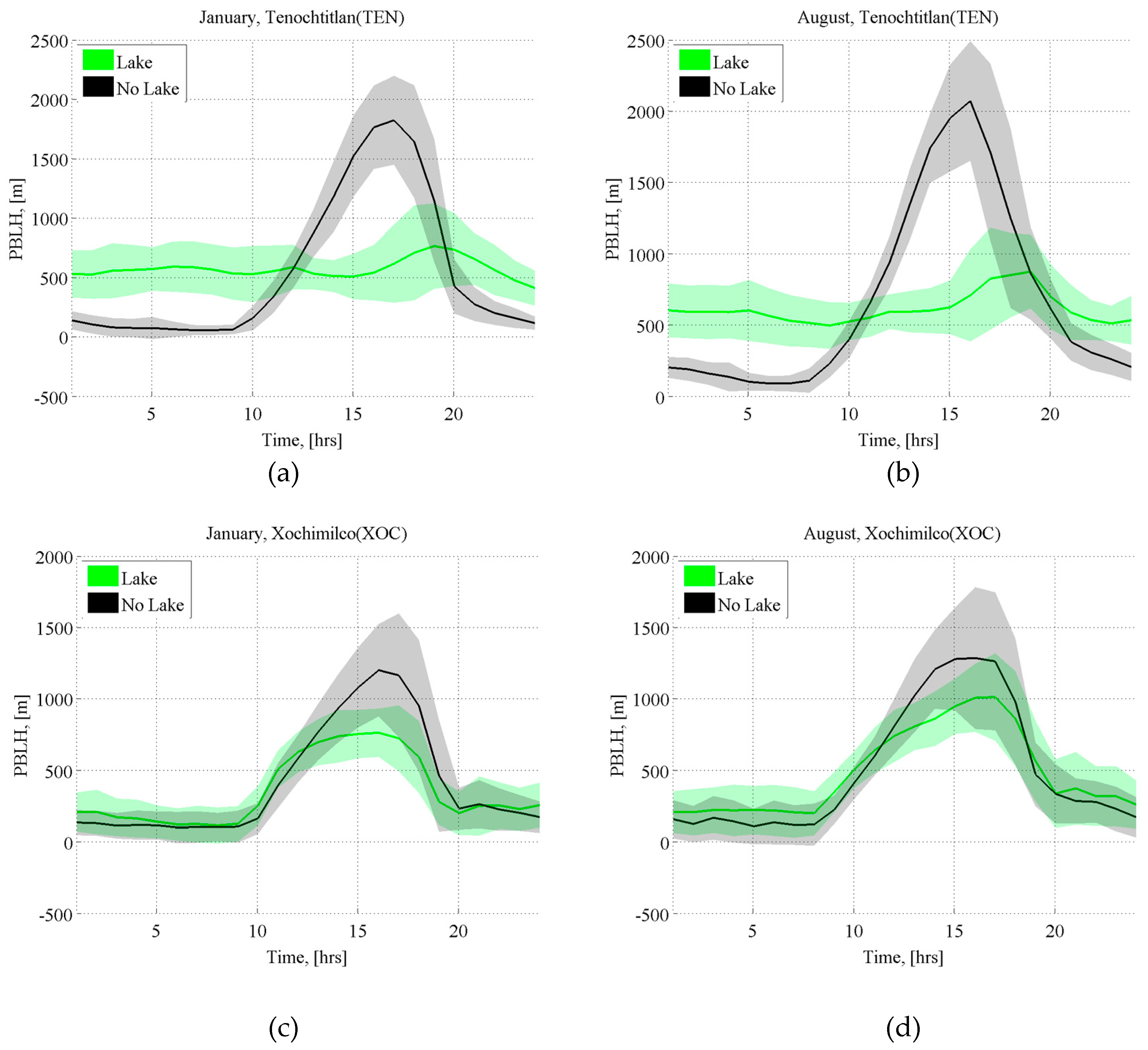
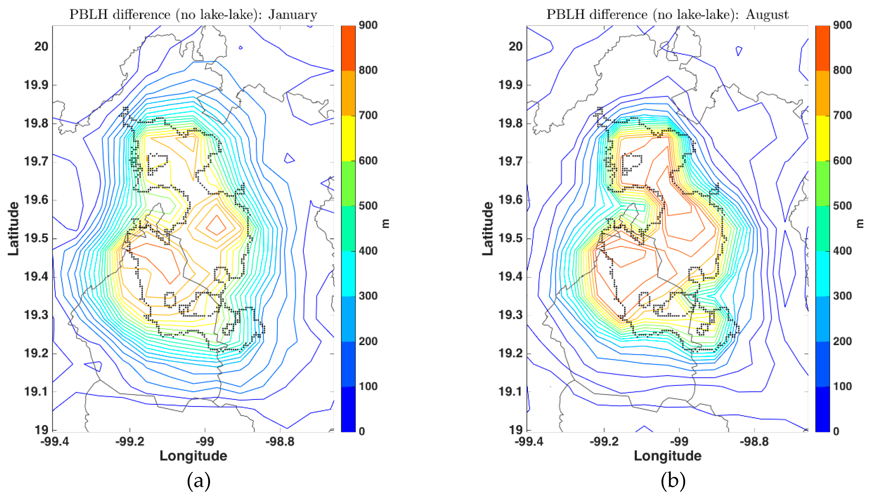
3.3. Planetary Boundary Layer Height (PBLH)
4. Discussion
5. Conclusions
Author Contributions
Funding
Acknowledgments
Conflicts of Interest
References
- Huang, A.; Wang, J.; Dai, Y.; Yang, K.; Wei, N.; Wen, L.; Wu, Y.; Zhu, X.; Zhang, X.; Cai, S. Evaluating and improving the performance of Three 1-D lake models in a large deep lake of the Central Tibetan Plateau. J. Geophys. Res. Atmos. 2019, 124, 3143–3167. [Google Scholar] [CrossRef] [PubMed]
- Notaro, M.; Holman, K.; Zarrin., A.; Fluck, E.; Vavrus, S.; Bennington, V. Influence of the Laurentian Great Lakes on regional climate. J. Clim. 2013, 26, 789–804. [Google Scholar] [CrossRef]
- Ruiz-Angulo, A.; López-Espinoza, E. Estimación de la respuesta térmica de la cuenca lacustre del Valle de México en el siglo XVI: Un experimento numérico. Bol. Soc. Geol. Mex. 2015, 67, 215–225. [Google Scholar] [CrossRef]
- Xu, L.; Liu, H.; Du, Q.; Wang, L. Evaluation of the WRF-lake model over a highland freshwater lake in southwest China. J. Geophys. Res. Atmos. 2016, 121, 13–989. [Google Scholar] [CrossRef]
- Oke, T.; Spronken-Smith, R.; Jáuregui, E.; Grimmond, C. The energy balance of central Mexico City during the dry season. Atmos. Environ. 1999, 33, 3919–3930. [Google Scholar] [CrossRef]
- Jazcilevich, A.; Fuentes, V.; Jauregui, E.; Luna, E. Simulated urban climate response to historical land use modification in the basin of Mexico. Clim. Chang. 2000, 44, 515–536. [Google Scholar] [CrossRef]
- Jáuregui, E. Heat island development in Mexico City. Atmos Environ. 1997, 31, 3821–3831. [Google Scholar] [CrossRef]
- Jáuregui, E. Impact of land-use changes on the climate of the Mexico City Region. Investig. Geogr. 2004, 55, 46–60. [Google Scholar] [CrossRef]
- Jáuregui, E.; Romales, E. Urban effects on convective precipitation in Mexico City. Atmos Environ. 1996, 30, 3383–3389. [Google Scholar] [CrossRef]
- Ochoa, C.; Quintanar, A.; Raga, G.; Baumgardner, D. Changes in intense precipitation events in Mexico City. J. Hydrometeorol. 2015, 16, 1804–1820. [Google Scholar] [CrossRef]
- Gu, H.; Shen, X.; Jin, J.; Xiao, W.; Wang, Y.W. An application of a 1-D thermal diffusion lake model to Lake Taihu. Acta Meteorol. Sin. 2013, 71, 719–730. [Google Scholar]
- Sharma, A.; Huang, H.; Zavialov, P.; Khan, V. Impact of desiccation of Aral Sea on the regional climate of Central Asia using WRF model. Pure. Appl. Geophys. 2018, 175, 465–478. [Google Scholar] [CrossRef]
- Ma, Y.; Yang, Y.; Qiu, C.; Wang, C. Evaluation of the WRF-lake model over two major freshwater lakes in China. J. Meteorol. Res. 2019, 33, 219–235. [Google Scholar] [CrossRef]
- Koseki, S.; Mooney, P.A. Influences of Lake Malawi on the spatial and diurnal variability of local precipitation. Hydrol. Earth Syst. Sci. 2019, 23, 2795–2812. [Google Scholar] [CrossRef] [Green Version]
- Diallo, I.; Giorgi, F.; Stordar, F. Influence of Lake Malawi on regional climate from a double-nested regional climate model experiment. Clim. Dyn. 2018, 50, 3397–3411. [Google Scholar] [CrossRef]
- Mallard, M.; Nolte, C.; Spero, T.; Bullock, O.; Alapaty, K.; Herwehe, J.; Gula, J.; Bowden, J. Technical challenges and solutions in representing lakes when using WRF in downscaling applications. Geosci. Model. Dev. 2015, 8, 1085–1096. [Google Scholar] [CrossRef] [Green Version]
- Gu, H.; Jin, J.; Wu, Y.; Ek, M.B.; Subin, Z.M. Calibration and validation of lake surface temperature simulations with the coupled WRF-lake model. Clim. Chang. 2015, 129, 471–483. [Google Scholar] [CrossRef]
- Benson-Lira, V.; Georgescu, M.; Kaplan, S.; Vivoni, E. Loss of a lake system in a megacity: The impact of urban expansion on seasonal meteorology in Mexico City. J. Geophys Res. Atmos. 2016, 121, 3079–3099. [Google Scholar] [CrossRef]
- Sanders, W.; Parsons, J.; Santley, R. The Basin of Mexico: Ecological Processes in the Evolution of A Civilization; Academic Press: New York, NY, USA, 1979. [Google Scholar]
- Lozano-García, M.; Ortega-Guerrero, B.; Caballero-Miranda, M.; Urrutia-Fucugauchi, J. Late Pleistocene and Holocene paleoenvironments of Chalco lake, central Mexico. Quat. Res. 1993, 40, 332–342. [Google Scholar] [CrossRef]
- Tolstoy, P.; Fish, S.; Boksenbaum, M.; Vaughn, K.; Smith, C. Early sedentary communities of the Basin of Mexico. J. Field Archaeo. 1977, 4, 91–106. [Google Scholar] [CrossRef]
- Ezcurra, E. De las Chinampas a la Megalópolis: El Medio Ambiente en la Cuenca de México; Fondo de Cultura Económica: Ciudad de Mexico, Mexico, 1990. [Google Scholar]
- Niederberger-Betton, C. Paléopaysages et Archéologie pre-Urbaine du Bassin de Mexico; Centre D’études Mexicaines et Centraméricaines: Ciudad de Mexico, Mexico, 1987. [Google Scholar]
- Endfield, G. Climate and Society in Colonial Mexico: A Study in Vulnerability; Wiley-Blackwell: Chicester, UK, 2011. [Google Scholar]
- García, E. Situaciones climáticas durante el auge y la caída de la cultura teotihuacana. Investig. Geogr. 1974, 5, 35–69. [Google Scholar] [CrossRef]
- Jáuregui, E. Effects of revegetation and new artificial water bodies on the climate of northeast Mexico City. Energy Build. 1974, 15, 447–455. [Google Scholar] [CrossRef]
- Mas, J.; Velázquez, A.; Díaz-Gallegos, J.; Mayorga-Saucedo, R.; Alcántara, C.; Bocco, G.; Castro, R.; Fernández, T.; Pérez-Vega, A. Assessing land use/cover changes: A nationwide multidate spatial database for Mexico. Int. J. Appl Earth Obs. Geoinf. 2004, 5, 249–261. [Google Scholar] [CrossRef]
- López-Bravo, C.; Caetano, E.; Magaña, V. Forecasting summertime surface temperature and precipitation in the Mexico City metropolitan area: Sensitivity of the WRF model to land cover changes. Front. Earth Sci. 2018, 6, 6. [Google Scholar] [CrossRef]
- Lafragua, J.; Gutiérrez, A.; Aguilar, E.; Aparicio, J.; Mejía, R.; Santillan, O.; Suárez, M.A.; Preciado, M. Balance hídrico del valle de México. In Anuario 2003; Gómez, M.A., Cruz, F., Wagner, A.I., Pineda, V.M., Requejo, A., Robles, B., Villavicencio, F.J., Eds.; Instituto Mexicano de Tecnología del Agua: Jiutepec, Mexico, 2003; pp. 40–46, ISBN-968-5536-38-4. [Google Scholar]
- Meza-Carreto, J. Evaluación del Desempeño del Modelo WRF para Reproducir las Variaciones de la Temperatura en México durante la Década de los 80. Master’s Thesis, Universidad Nacional Autónoma de México, Ciudad de Mexico, Mexico, 12 November 2018. [Google Scholar]
- López-Méndez, V. Análisis del Evento Meteorológico Relacionado con la Inundación de Tabasco del 2009. Master’s Thesis, Universidad Nacional Autónoma de México, Ciudad de Mexico, Mexico, 30 June 2009. [Google Scholar]
- Jurado de Larios, O.E. Sensibilidad del Modelo WRF ante Condiciones Iniciales y de Frontera: Un Estudio de Caso en el Valle de México. Master’s Thesis, Universidad Nacional Autónoma de México, Ciudad de Mexico, Mexico, 27 June 2017. [Google Scholar]
- López-Espinoza, E.D.; Zavala-Hidalgo, J.; Mahmood, R.; Gómez-Ramos, O. Assessing the Land Use and Land Cover Data Representation on Weather Forecast Quality: A Case Study in central Mexico. Meteorol. Atmos. Phys. under review.
- Reporte del Clima en México. Available online: https://smn.conagua.gob.mx/es/climatologia/diagnostico-climatico/reporte-del-clima-en-mexico (accessed on 7 September 2019).
- Meteorología/Grupo Interacción Océano-Atmósfera. Available online: http://grupo-ioa.atmosfera.unam.mx/pronosticos/index.php/meteorologia (accessed on 11 September 2019).
- Kalnay, E. Atmospheric Modeling, Data Assimilation and Predictability; Cambridge University Press: New York, NY, USA, 2003. [Google Scholar]
- Kain, J. The Kain–Fritsch convective parameterization: An update. J. Appl. Meteorol. 2004, 43, 170–181. [Google Scholar] [CrossRef]
- Skamarock, W.; Klemp, J.; Dudhia, J.; Gill, D.; Barker, D.; Wang, W.; Powers, J. A Description of the advanced research WRF version 2. NCAR Tech. Note 2005, 468. [Google Scholar] [CrossRef]
- Zhang, Y.; Dubey, M.K.; Olsen, S.C.; Zheng, J.; Zhang, R. Comparisons of WRF/Chem simulations in Mexico City with ground-based RAMA measurements during the 2006-MILAGRO. Atmos. Chem. Phys. 2009, 9, 3777–3798. [Google Scholar] [CrossRef] [Green Version]
- Chen, F.; Dudhia, J. Coupling an advanced land surface–hydrology model with the Penn State–NCAR MM5 modeling system. Part I: Model implementation and sensitivity. Mon. Weather Rev. 2001, 129, 569–585. [Google Scholar] [CrossRef]
- Loveland, T.; Reed, B.; Brown, J.; Ohlen, D.; Zhu, Z.; Yang, L.; Merchant, J. Development of a global land cover characteristics database and IGBP DISCover from 1 km AVHRR data. Int. J. Remote Sens. 2000, 21, 1303–1330. [Google Scholar] [CrossRef]
- Oleson, K.; Lawrence, D.; Gordon, B.; Flanner, M.; Kluzek, E.; Peter, J.; Levis, S.; Swenson, S.; Thornton, E.; Feddema, J.; et al. Technical description of version 4.0 of the Community Land Model (CLM). NCAR Tech. Note 2010, 478. [Google Scholar] [CrossRef]
- Subin, Z.; Riley, W.; Mironov, D. An improved lake model for climate simulations: Model structure, evaluation, and sensitivity analyses in CESM1. J. Adv. Model. Earth Syst. 2012, 4, 1–27. [Google Scholar] [CrossRef]
- Thiery, W.; Stepanenko, V.; Fang, X.; Jöhnk, K.; Li, Z.; Martynov, A.; Perroud, M.; Subin, Z.; Darchambeau, F.; Mironov, D.; et al. LakeMIP Kivu: Evaluating the representation of a large, deep tropical lake by a set of one-dimensional lake models. Tellus A Dyn. Meteorol. Oceanogr. 2014, 66, 21390. [Google Scholar] [CrossRef]
- Raynal-Villasenor, J.A. The Remarkable Hydrological Works of the Aztec Civilization. Available online: http://hydrologie.org/redbooks/a164/iahs_164_0003.pdf (accessed on 7 September 2019).
- Cosgrove, A.; Berkelhammer, M. Downwind footprint of an urban heat island on air and lake temperatures. NPJ Clim. Atmos Sci. 2018, 1, 46. [Google Scholar] [CrossRef] [Green Version]
- Koster, R.; Suarez, M.; Liu, P.; Jambor, U.; Berg, A.; Kistler, M.; Reichle, R.; Rodell, M.; Famiglietti, J. Realistic initialization of land surface states: Impacts on subseasonal forecast skill. J. Hydrometeorol. 2004, 5, 1049–1063. [Google Scholar] [CrossRef]
- Zola, R.; Bengtsson, L. Long-term and extreme water level variations of the shallow Lake Poopó, Bolivia. Hydrol. Sci. J. 2006, 51, 98–114. [Google Scholar] [CrossRef]
- Lauwaet, D.; Van Lipzig, N.; Van Weverberg, K.; De Ridder, K.; Goyens, C. The precipitation response to the desiccation of Lake Chad. Q. J. R. Meteorol. Soc. 2012, 138, 707–719. [Google Scholar] [CrossRef]
- Hartmann, D.; Tank, A.; Rusticucci, M.; Alexander, L.; Brönnimann, B.; Charabi, Y.; Dentener, F.; Dlugokencky, E.; Easterling, D.; Kaplan, A.; et al. Observations: Atmosphere and Surface. Climate Change 2013 the Physical Science Basis: Working Group I Contribution to the Fifth Assessment Report of the Intergovernmental Panel on Climate Change; Cambridge University Press: New York, NY, USA, 2013. [Google Scholar]
- Thiery, W.; Davin, E.L.; Seneviratne, S.I.; Bedka, K.; Lhermitte, S.; Van Lipzig, N.P. Hazardous thunderstorm intensification over Lake Victoria. Nat. Commun. 2016, 7, 12786. [Google Scholar] [CrossRef] [Green Version]


| Analyzed Sites | January | August | ||||||
|---|---|---|---|---|---|---|---|---|
| No-Lake | Lake | No-Lake | Lake | |||||
| Daily mm/h | Accum. mm/day | Daily mm/h | Accum. mm/day | Daily mm/h | Accum. mm/day | Daily mm/h | Accum. mm/day | |
| TEN | 0.01 | 0.12 | 0.01 | 0.31 | 0.39 | 9.47 | 0.56 | 13.54 |
| TEO | 0 | 0.08 | 0 | 0.07 | 0.17 | 4.02 | 0.31 | 7.38 |
| TEX | 0 | 0.01 | 0.01 | 0.33 | 0.16 | 3.86 | 0.25 | 5.91 |
| XOC | 0.01 | 0.19 | 0.03 | 0.64 | 0.26 | 6.26 | 0.57 | 13.73 |
| CHA | 0 | 0.03 | 0.01 | 0.34 | 0.13 | 3.07 | 0.27 | 6.39 |
| CUL | 0 | 0.08 | 0.03 | 0.64 | 0.23 | 5.41 | 0.57 | 13.66 |
| ZUM | 0.01 | 0.19 | 0.01 | 0.33 | 0.31 | 7.30 | 0.35 | 8.44 |
| Average | 0 | 0.10 | 0.02 | 0.38 | 0.23 | 5.63 | 0.41 | 9.87 |
© 2019 by the authors. Licensee MDPI, Basel, Switzerland. This article is an open access article distributed under the terms and conditions of the Creative Commons Attribution (CC BY) license (http://creativecommons.org/licenses/by/4.0/).
Share and Cite
López-Espinoza, E.; Ruiz-Angulo, A.; Zavala-Hidalgo, J.; Romero-Centeno, R.; Escamilla-Salazar, J. Impacts of the Desiccated Lake System on Precipitation in the Basin of Mexico City. Atmosphere 2019, 10, 628. https://doi.org/10.3390/atmos10100628
López-Espinoza E, Ruiz-Angulo A, Zavala-Hidalgo J, Romero-Centeno R, Escamilla-Salazar J. Impacts of the Desiccated Lake System on Precipitation in the Basin of Mexico City. Atmosphere. 2019; 10(10):628. https://doi.org/10.3390/atmos10100628
Chicago/Turabian StyleLópez-Espinoza, Erika, Angel Ruiz-Angulo, Jorge Zavala-Hidalgo, Rosario Romero-Centeno, and Josefina Escamilla-Salazar. 2019. "Impacts of the Desiccated Lake System on Precipitation in the Basin of Mexico City" Atmosphere 10, no. 10: 628. https://doi.org/10.3390/atmos10100628