1. Introduction
The detection and prediction of tsunami waves is an urgent task of modern geophysics [
1,
2]. Among the various approaches to the problem, a set of investigations aimed at studying the ocean–atmosphere–ionosphere connection is being distinguished. Such an approach allows monitoring this formidable phenomenon using satellite communication systems that provide tomographic images of the distribution of the total electron concentration in the region of the dangerous activity of underwater earthquakes and, accordingly, tsunamis [
3].
In [
4], convincing arguments were presented in favor of the fact that phenomena occurring in the oceans are an important source of waves in the thermosphere. The transmitting link of the disturbance from surface ocean waves is the atmosphere. The tsunami wave disturbs in the atmosphere acoustic and internal gravitational waves [
5], the propagation of which at the heights of the thermosphere is accompanied by the transport of plasma along the lines of force. This in turn affects the total electron concentration [
6,
7,
8,
9]. Thereby, the solution of the problem of the propagation of the waves initiated by water–air interface boundary conditions proves to be important both in the diagnostics of atmospheric effects and for the detection of tsunami waves at the initial stage [
10]. The solution of the problem of propagating such exited acoustic waves is important since observations show that “the first arrival of a transient signal of tsunami-induced waves occurs at a 100-km altitude just 5 min after the tsunami is generated” [
11]. In this paper [
11], the authors presented two 2D models. The first one is the inelastic fluid model, the analytical-numerical model in which the background state of the atmosphere is modeled as two-layers with the matching conditions at the interface. These conditions lead to the appearance of a reflected wave. The second one is the compressible fluid model for acoustic-gravity waves, which the authors solved numerically.
In [
12], the authors simulated numerically the propagation of 2D-dimensional, linear AGW in an atmosphere including vertically-varying stratification and horizontal background winds. The work [
9] considered the tsunami–atmosphere–ionosphere coupling mechanism and numerically solved for atmospheric and ionospheric effects. The authors in [
13] simulated the ionospheric responses to infrasonic-acoustic waves, using the compressible atmospheric dynamics model. The paper [
14] described the propagation of gravity waves with dissipation. In [
8], the summation of the extended seismic normal modes was used to retrieve the tsunami signature in the ocean, atmosphere, and ionosphere. Such, mainly numerical, investigations present different important aspects of the phenomenon in much detail [
15].
The problem of the propagation of long acoustic waves in the atmosphere has a significant history [
5,
10,
16]. Since the wavelength is much less than the main parameter of the inhomogeneity of the unperturbed gas, the so-called atmospheric scale height (
H) [
17] can be employed. Such an approximate description enables the use of the concepts of a homogeneous propagation medium, considering
H as a parameter. On the other hand, taking into account weak heterogeneity, methods similar to the semiclassical approximation of quantum mechanics [
18] can be adopted. If the spectrum of wavelengths significantly overlaps with values of order
H, it is necessary to resort to splitting the atmosphere into horizontal layers. In this case, the stratification is to be considered exponential [
19].
Important results were obtained for the exponential atmosphere within the linear theory [
5] and for the non-linear generalization in various orders of magnitude of non-linearity [
20,
21]. For instance, the dispersion relations were derived, which provided the basis for the developed concepts and practical recommendations for geophysics. Here, the Cauchy problem was considered, with the appropriate set of initial conditions.
In our work, we study the formulation and analytical solution of the problem of purely acoustic perturbations and their ionospheric effect. Such a problem is the propagation of a plane atmospheric wave, which, obviously, does not contain internal gravitational waves, being 2D phenomenon by definition.
Thus, the problem of the propagation of the waves exited by time-dependent boundary condition is considered in this work, where the generating mode is specified at the water–air interface. The atmosphere is traditionally divided into layers with constant
H similar to [
19]. This type of problem may be interesting for modeling the high-altitude effect of surface waves in the ocean. This is especially important for waves such as tsunamis with a large amplitude and space scale [
4]. Based on the large horizontal scale of the surface waves under consideration, the one-dimensional model of the atmosphere is adopted and combined along with projecting the general solution of the problem of the propagation of the boundary condition impact perturbation to the subspace of unidirectional waves.
The Fourier method is employed to solve the basic equations and deliver the transformation from the time domain to the frequency domain. The solution of the resulting ordinary differential equations transforms to the time domain by inverse Fourier transform to obtain the final integral form. The corresponding integral contains a rapidly-oscillating function, which paves the way for further analysis.
As a natural path to the approximate evaluation of the resulting integral, the method of the stationary phase is adopted and defines the group velocity and amplitude functions. An explicit formula for the fluid velocity field enables the transformation to the electron density evolution equation.
As the final step of the proposed method, an effective analytical representation for ionosphere electron density is used [
6,
7]. It is an explicit solution of the diffusion equation with the coefficient representing the acoustic wave. The set of the explicit resulting formulas forms the base for a fast algorithm for a tsunami diagnostic model.
4. Building a Multi-Layered Model Solution
According to the multilayer model of the atmosphere shown in
Figure 1, the average atmospheric scale height will change during the transition from one layer to another, and therefore, the average temperature and density do change. Hence, the cross-linking of the solutions at the layer boundary will be based on the continuity of entropy [
26] to keep the heat flux continuous. We rewrite the relation (
6) for the case of the
n-layered model:
Further, the indices will denote the layer number, i.e., is the atmospheric scale height in the n-layer.
The cross-linking condition is such that:
where
is the height of the interface between
n- and
n+1-layers and
. Therefore, for the variables, we use have:
or it can be rewritten as:
According to (
9), we write:
or:
The next step involves the velocity field:
where
can be calculated as:
The variables
and
are related to
and
by the inverse Fourier transform:
Using (
57):
and (
52) and (
55), we have:
Furthermore, using the link (
19), we arrive at:
According to the results of the previous subsection’s solution in the first layer
, it is derived:
where
is the atmospheric scale height in the first layer
; or we can rewrite it as:
where
; or as the recurrent formula for the calculation:
Using the last formula for (
61), we obtain:
where:
Finally, the complete expression for the coefficients
yields:
The recurrent formulas for the calculation of solutions in the “
n”-layer are found with (
63):
where:
which accomplish the
n-layer model of the acoustic wave in
- representation.
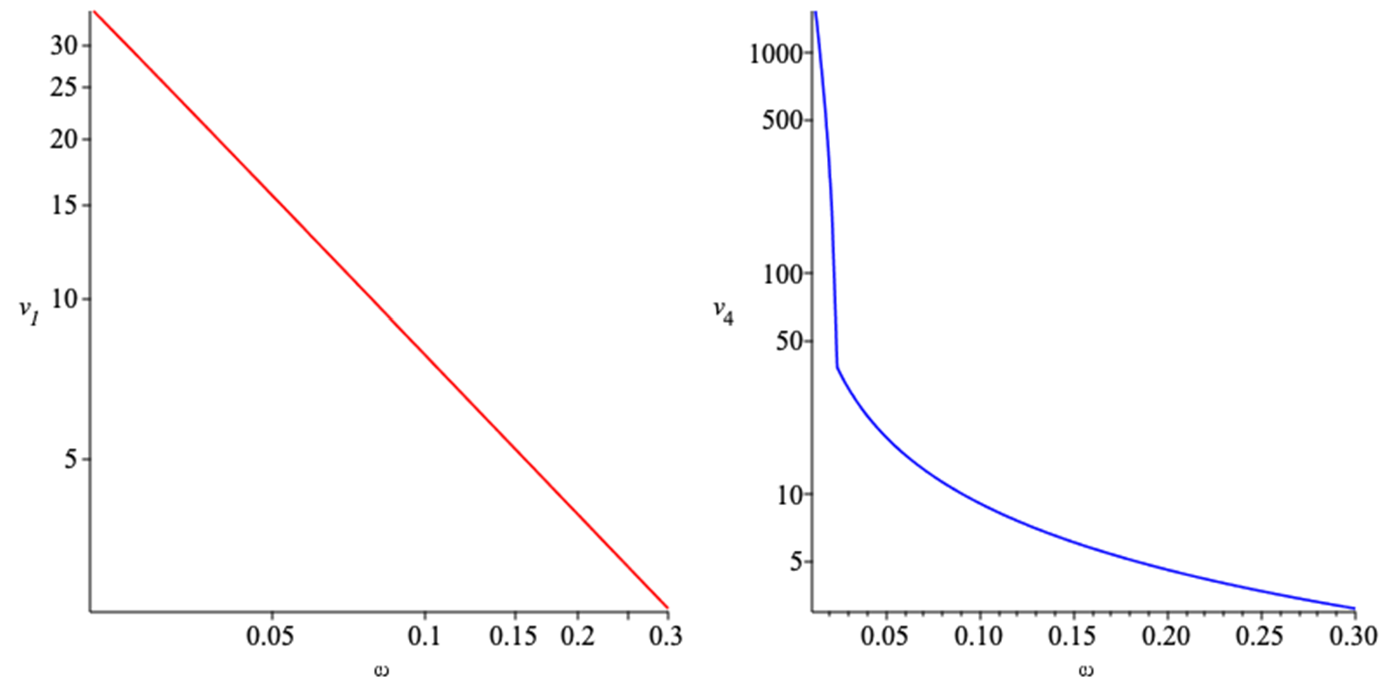
The result is illustrated by the plots in
Figure 2 for the velocity field of the acoustic wave in the
-domain:
Solution and Estimations in the Time Domain
Using the inverse Fourier transform, we find recurrence formulas in the time domain:
The integrand of (
76)–(
78) contains rapidly-oscillating function
at the range of
. It allows applying asymptotic representation for the integral by conventional stationary phase approximation via the stationary point frequency
. Generally, having the integral:
the conventional asymptotic expression yields:
Here, the phase term
is “stationary” when:
The root of this equation gives the dominant frequency
for certain
z and
t. In the case of (
76), for
,
The stationary phase approximation (
80) gives the explicit expression for the velocity
that is used for the calculations of the electron density perturbation after arrival time
. The solution properties were demonstrated by the explicit formula for the integral (
76) obtained in the stationary phase method asymptotic by means of the dispersion function
. It gives group velocities
for each layer and the wave-trains’ amplitude envelope form via the classic expression based on
. The resulting representation for the electron concentration is derived by the explicit expression for the solution of the diffusion equation at [
7,
27].
6. Discussion: Comparison
Due to the exponential growth of the amplitude with increasing altitude above sea level, even small disturbances (for example, for speeds of the order of 25 cm/s) at sea level increase at the altitudes of the ionosphere, which gives a gas velocity amplitude over 200 m/s, cf. [
11]. This guarantees the possibility to use the model in tsunami diagnostics and the eventual prognosis of the wave impact at the seashore.
It is impossible to compare the results of our modeling and others’ directly because for such a situation, both models should have close mathematical statements of the problem and similar outputs. Some important features of the results, however, may be disclosed. Most closed problems were considered in the paper [
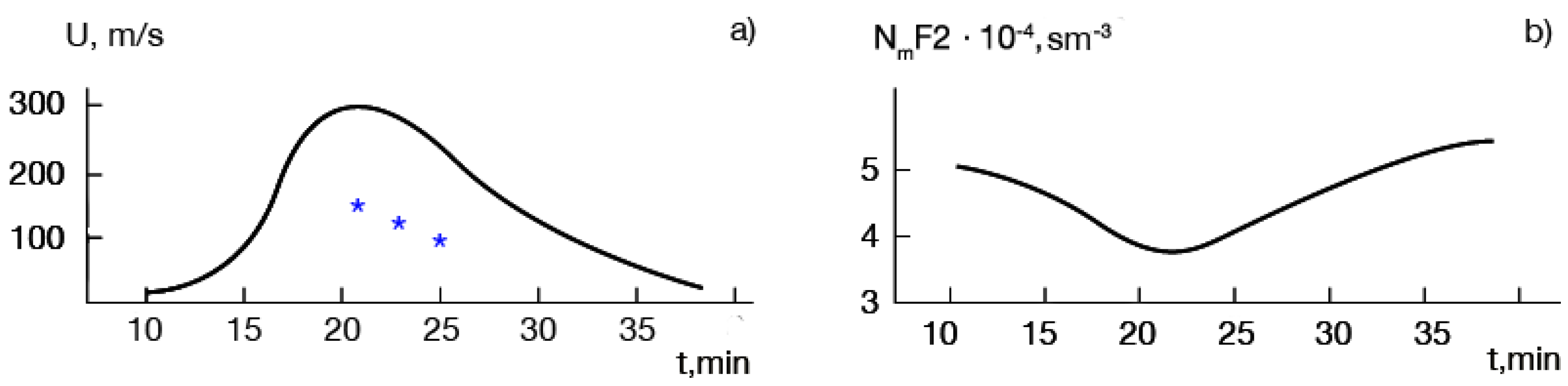
13], where infra-sound propagation was studied. This is also the case in our work. The vertical profiles of the velocity for three moments of time given in Figure 11 of [
13] allow estimating the amplitude at heights of about 300 km. We put the values in
Figure 3a as stars. It is difficult to give a more detailed comparison between our results, due to the mentioned reasons. The order of amplitudes, at least, is the same.
Another important possibility is in comparison with the pulse arrival times
at a prescribed height, estimated by the summation of the times
(
, the group velocity in
n-layer). This was supported by information about the measurements in the paper [
11]. More precisely, the arrival time was estimated by the condition
and evaluation of the time delay via the layer group velocities
. For the height of 100 km, it gives the value
s, the sum of time delays for the first layers, which approximately corresponds to the result of the simulations and experiments given in [
11].
The third one is related to ionosphere perturbations; see again [
13]. The simulations show the variation of the electron density at the
F-layer of about 8–10% (Figure 10 of [
13]), which is in rather good correspondence with our estimations shown in
Figure 3b. The lesser infra-sound wave amplitudes, shown in
Figure 3a, left, produce lesser electron variations against ours, that is about 20%.
7. Conclusions
The main result of this paper is the recurrent formula that connects the exponentially-stratified adjacent layers of a planetary atmosphere. It allows constructing an algorithm for the solution of an acoustic wave propagation problem, starting with the appropriate time-dependent boundary condition at the planetary surface. The crucial element of this model is the projection procedure, derived for the z-evolution operator for the interface of layers. Such a procedure eliminates the down-directed wave and properly establishes the transition from the “n” layer to the next one “n + 1”. The model is applied to the problem of an acoustic wave initiated by a long ocean wave. The choice of the boundary regime is made on the basis of empirical data analysis. A model of the acoustic wave generated by the earthquake may be built in a similar fashion. The asymptotic expression of the resulting integrals by the large parameter (z) gives an explicit expression for the fluid velocity field at arbitrary heights in the frame of the proposed model. In return, it allows employing the explicit formula for the electron concentration at ionosphere layers.
Finally, combining the analytical formulas creates the basis for the algorithm that can evaluate the ionospheric effect very quickly. Such a model for tsunami or earthquake diagnostics may be beneficial.
An important step towards greater sophistication of the proposed 1D model would be to refine the boundary regime more appropriately to represent the tsunami wave. For instance, in [
20,
28], function (29), multiplied by a trigonometric function, was proposed. Such a modification allows computing the Fourier image and adjusting the working formula (34). The work will continue with the calculation of the ionospheric effect at altitudes above the second layer, given that the formalism is transferred to the next layer almost automatically.


