Article

Combinatorial Optimization for WRF Physical Parameterization Schemes: A Case Study of Three-Day Typhoon Simulations over the Northwest Pacific Ocean

1
State Key Laboratory of Earth Surface Processes and Resource Ecology, Faculty of Geographical Science, Beijing Normal University, Beijing 100875, China
2
State Key Laboratory of Numerical Modeling for Atmospheric Sciences and Geophysical Fluid Dynamics, Institute of Atmospheric Physics, Chinese Academy of Sciences, Beijing 100029, China
3
State Key Laboratory of Severe Weather, Chinese Academy of Meteorological Sciences, Beijing 100081, China
*
Author to whom correspondence should be addressed.
Atmosphere 2019, 10(5), 233; https://doi.org/10.3390/atmos10050233
Submission received: 21 March 2019 / Revised: 18 April 2019 / Accepted: 23 April 2019 / Published: 1 May 2019
(This article belongs to the Special Issue Weather Research and Forecasting (WRF) Model)

Abstract

:
Quantifying a set of suitable physics parameterization schemes for the Weather Research and Forecasting (WRF) model is essential for obtaining highly accurate typhoon forecasts. In this study, a systematic Tukey-based combinatorial optimization method was proposed to determine the optimal physics schemes of the WRF model for 15 typhoon simulations over the Northwest Pacific Ocean, covering all available schemes of microphysics (MP), cumulus (CU), and planetary boundary layer (PBL) physical processes. Results showed that 284 scheme combination searches were sufficient to find the optimal scheme combinations for simulations of track (km), central sea level pressure (CSLP, hPa), and 10 m maximum surface wind (10-m wind, m s−1), compared with the 700 sets of full combinations (i.e., 10 MP × 7 CU × 10 PBL). The decrease in the typhoon simulation error (i.e., root mean square error between simulation and observations) with this optimal scheme combination was 34%, 33.92%, and 25.67% for the track, CSLP, and 10-m wind, respectively. Overall, the results demonstrated that the optimal scheme combination yields reasonable results, and the Tukey-based optimization method is very effective and efficient in terms of computational resources.

Graphical Abstract

1. Introduction

Typhoons are strong cyclonic vortexes stemming from the tropical oceans under conditions of high sea-surface temperatures and weaker shear winds. With their frequent occurrences, extremely strong winds, precipitations, and occasional storm surges, typhoons cause considerable human, environmental, and financial losses, and they represent a severe threat to the people and environment of East Asia, such as in China, Japan, Taiwan, and the Philippines. Accurate forecasting of typhoon tracks and intensity is crucial to ensure the preparedness of the affected countries, and to enable mitigation measures to be implemented.
With the increase in observation tools and the development of supercomputing technology, mesoscale numerical weather prediction (NWP) models have become essential tools for forecasting the evolution of typhoons. The forecast results of the mesoscale models usually yield large errors due to the uncertainties inherent to initialization fields of the global model products, and the physical representations of the mesoscale model itself. Taking the Weather Research and Forecasting (WRF) model [1] as an example, the process of how to reduce the typhoon simulation errors in existing literature is briefly listed as follows.
Several typhoon initialization methods exist to eliminate the uncertainty of the initial values, such as building a bogus vortex method [2,3,4,5], bogus data assimilation method [6,7,8,9,10], and a dynamical initialization method [11,12,13]. The uncertainty of the models’ physical representation is another important source of simulation error, and many studies have focused on improvements to the model’s physical processes for better simulation of tropical cyclones. For instance, the tropical cyclone prediction accuracy was improved by adjusting the roughness parameterization description and other critical parameters related to surface layer processes [14,15,16]. Moreover, in the description of the cumulus process, a new formula for the convective temperature perturbation of the Kain–Fritsch scheme was proposed to improve the typhoon simulations [17]. Another study found that the ocean feedback process (i.e., accurate environmental wind shear) is crucial to attaining a skillful typhoon intensity forecasting [18]. Lastly, hurricane prediction models with finer grid spacing, such as the coupled boundary layer air–sea transfer hurricane model [19], have been developed to resolve the simulation of the typhoons eye and eyewall at a ~1 km grid spacing. This study attempts to minimize the uncertainties due to the physical representation of the model itself rather than the initialization fields.
The WRF model provides several parameterization schemes to be selected for the description of each physics option, such as microphysics (MP), cumulus (CU), and the planetary boundary layer (PBL). Therefore, much effort was made to select the more representative physics parameterization schemes for reproducing the typhoons/hurricanes track and intensity [20,21,22,23,24,25,26,27,28,29]. However, these efforts present two disadvantages. Firstly, these experiments focused only on a single typhoon/hurricane case. For example, Raju et al. [20], via a scheme sensitivity analysis, determined more suitable parameterization schemes (e.g., the National Center for Environmental Prediction(NCEP) operational cloud MP scheme, Kain–Fritsch CU scheme, and the Yonsei University PBL scheme) to reproduce the track and intensity of typhoon “Nargis” over the Bay of Bengal using the WRF model. Islam et al. [29] analyzed the sensitivity of the WRF’s MP, CU, and PBL physics schemes on the simulation of super typhoon “Haiyan”, and they found that the CU scheme was helpful for typhoon intensity prediction. Secondly, not all the schemes were assessed, regardless of the single- or multi-event nature of the simulation. Osuri et al. [22] analyzed three CU and two PBL schemes to quantify the optimal scheme combination for the simulations of five typhoons over the Indian Ocean. Li [25] assessed the effect of CU schemes on the simulations of 20 typhoon cases using only three of all the six parameterization schemes, while the other physics schemes were fixed. Srinivas et al. [26] assessed 13 scheme combinations with four CU, three MP, and three PBL schemes to quantify the optimal WRF combination simulations for 21 typhoons. However, some better schemes may be overlooked due to the lack of a comprehensive evaluation for all the schemes beforehand.
It is noted that there are some studies on scheme combination selection. For instance, Zhang et al. [30] assessed the uncertainties of the Noah–MP land surface model consisting of 4608 selected physical scheme combinations, using the natural selection approach and the Tukey’s test method. The results demonstrated that selection results for the Tukey’ test method were consistent with the natural selection approach. However, this study only focused on the simulation of the land surface heat flux at Dali site in the Tibetan Plateau (TP) region, and all of the Noah–MP schemes were simulated.
In the WRFv3.6.1, a total of 21 MP schemes, 11 CU schemes, and 12 PBL schemes exist. Regardless of the selection of other physics schemes (e.g., land surface model, longwave, or shortwave radiation, etc.), 2772 (21 × 11 × 12) scheme combinations need to be tested to quantify the best one for typhoon simulations. Considerable computational resources are required to find the optimized scheme and it is a very challenging task, which is why only the representative or commonly used physics parameterization schemes were combined in the previous studies. In this study, we attempt to propose a systematic combinatorial optimization method for all the WRF physics schemes available, which can search for the optimal configuration using the least number of combinatorial experiments rather than all the combinatorial experiments. The literature mentioned above revealed that typhoon simulation in the WRF model is mostly sensitive to the three physics modules of CU, MP, and PBL, and only the combination of these three modules is tested, with other schemes being fixed.
This paper is organized as follows. Section 2 presents the data used and the methodology of the scheme combinatorial optimization, Section 3 shows the optimization results and analyses, Section 4 discusses the reasonableness of the optimal scheme combinations obtained, and the conclusions are presented in the last section.

2. Data and Methodology

2.1. Data for Scheme Combination Optimization

To obtain reasonable optimal scheme combinations for typhoon simulations, 15 typhoon cases from 2011 to 2015 were simulated in this study. All of these typhoons generated over the Northwest Pacific Ocean and passed through the areas of Southeast Asia and the southeast coastal areas of China. Here, only three-day tracks for each typhoon were simulated. The three-day tracks of the 15 typhoons are shown in Figure 1, and the typhoons’ Chinese number ID, name, and simulation period are listed in Table 1. For the three days, all the typhoons only occurred over the ocean and experienced a process of strengthening and weakening. The corresponding typhoon observation dataset was obtained from the China Meteorological Administration (CMA)-Shanghai Typhoon Institute (STI) best track dataset for tropical cyclones over the western North Pacific [31]. It included track (km), central sea level pressure (CSLP, hPa), and 10-m maximum surface wind (10-m wind, m s−1) data.

2.2. WRF Model Configuration for Typhoon Simulations

The 15 typhoons were simulated using the Advanced Research WRF (WRF-ARW) version 3.6.1 [32]. A two-grid horizontally nested domain was set up. The outer domain was located within 3.13° S−37.06° N and 98.39°−151.81° E (see Figure 1), while the inner domain was an automatically moving nest based on an automatic vortex-following algorithm. This setup for the inner domain enabled the location of the tropical cyclone to be better tracked. The outer domain was made of 156 × 126 grid cells with a resolution of 36 km, and the inner domain consisted of 135 × 135 grid cells with a resolution of 12 km. The uniform time step was 180 s, for both the inner and outer domain simulations. The inner domain moved with the typhoon vortex, while the outer domain was fixed. Therefore, the outer domain should be defined to cover the three-day tracks of the 15 typhoons. The size of the inner domain occupied 1/3 of the outer domain, which enabled the moving inner domain located in the center of the outer domain to obtain more accurate simulation results. The space and time resolutions were specified based on the computation amount available for the WRF simulations on the scheme combination optimization. Additionally, the time step is usually chosen as being at least six times the space resolution of inner domain. Here, a 180 s time step was used to save the computational amount for one model run [33,34], which was critical to conducting the simulations of scheme combination optimization thereafter.
The lateral boundary condition of the outer domain was set by the NCEP Final (FNL) Operational Global reanalysis dataset [35], which was available at a 1° × 1° horizontal resolution and a 6 h interval. The outermost domain was not nudged, which may have had some negative effects on the simulation accuracies. However, the comparisons amongst the schemes were conducted under the same boundary data and boundary setting, making the results of the optimal schemes reasonable. The initial values for the simulations were obtained by interpolating the NCEP FNL data to the grid cells, and then by spinning up the model for 6 h. The default physics scheme followed the WRF setup from the CMA typhoon operational forecasting system. It included the WSM6 MP scheme [36], the Kain–Fritsch (new Eta) CU scheme [37], the Yonsei University (YSU) PBL scheme [38], the revised MM5 Monin–Obukhov surface layer (SF) scheme [39], the Dudhia shortwave scheme [40], the RRTM longwave scheme [41], and the Noah land-surface model [42]. Thereafter, these schemes were referred to as the default schemes of the WRF model. The default and optimization simulations used the above configurations except for the CU, MP, and PBL schemes.
The schemes of the three physics modules, including CU, MP, and PBL, available for the typhoon simulations were systematically assessed to find the optimal scheme combination. However, not all the schemes were suitable to the above simulation configuration. For instance, some schemes were difficult to freely match with the other physics schemes like the Milbrandt–Yau [43] and HUJI full and fast schemes in the MP physics module [44,45], the Zhang–McFarlane scheme [46] of the CU physics module, and the TEMF scheme [47] of the PBL physics module. Some schemes were only used to the nonhydrostatic mesoscale model (NMM) core of the WRF model, rather than the ARW core, like the simplified Arakawa–Schubert scheme [48] of the CU physics module and the GFS scheme [49] of the PBL physics module. Some schemes required a specialized simulation configuration, such as the Kessler scheme [50] for idealized cases, the Eta [51], the Goddard [52], and the four NSSL-serial schemes [53] for fine resolution (<5 km) simulations, as well as the Grell–Devenyi ensemble scheme [54] for the fixed nest. Excluding these unsuitable schemes, there remained 10 MP schemes, 7 CU schemes, and 10 PBL schemes that matched as suitable SF schemes. For the surface layer scheme, we used the ones recommended for use with the PBL option. The selected parameterization schemes for the three physics modules of the MP, CU, and PBL are listed in Table 2, in which “Num.” represents the scheme order defined in the physics. To distinguish the different Mellor–Yamada–Nakanishi–Niino level 2 (MYNN2) PBL scheme combinations, the 5(1), 5(2), and 5(3) designations for the PBL options represented the combinations of scheme (5) of the PBL (i.e., MYNN2) and the schemes (1), (2), and (3) of the SF, respectively. A similar naming standard was used for the 9(1) and 9(2) PBL options.
Except for the MP, CU, and PBL physics modules, only one parameterization scheme was employed for each of the other physical processes in the simulation. The unified Noah land surface scheme was used for the land surface module, and the rapid radiative-transfer model (RRTM) and Dudhia schemes were chosen as the long-wave and short-wave radiation modules, respectively.
The typhoon simulation errors for track, CSLP, and 10-m wind are respectively expressed as follows:
R M S E = 1 N i = 1 N t = 1 T j = 1 M ( s i m i , j t o b s i , j t ) 2 M T
where s i m i , j t and o b s i , j t represent the simulated and observed variables (track or CSLP or 10-m wind speed), at the jth observation point, and at time t for ith typhoon; M and T are the total numbers of observation points and time steps for the ith typhoon; N is the total number of typhoons. Here, the observation frequency was once each 6 h.

2.3. Data for the Validation of the Optimal Scheme Combination

Two independent typhoon cases from 2016 to 2017 were selected to test whether the optimal scheme combination obtained from the 15 typhoon simulations was effective in improving the other typhoon simulations. The two independent cases were the typhoon Megi assigned with the Chinese number ID 201617 and the typhoon Nesat assigned with the Chinese number ID 201709, and their simulation periods were 3 days. For the typhoon Megi, the simulation period was from 6 am on 24 September 2016 to 6 am on 27 September 2016; and for the typhoon Nesat, the simulation period was from 6 am on 27 July 2017 to 6 am on 30 July 2017. For each three-day typhoon simulation, the design of the domain and simulation and the forcing data source, were the same as the previous optimization simulations for the 15 typhoons, except for the schemes of the MP, CU and PBL physics. Here, the observation data of track, CSLP, and 10-m wind were still from the CMA-SIT best track dataset for tropical cyclones over the western North Pacific.

2.4. Optimization Method

2.4.1. Tukey’s Test Method

The combinatorial optimization of the WRF physics schemes was considered to be a discrete optimization problem, and in this study, the Tukey’s test method (also called the Tukey method) [55] was used to compare the difference in the population means of two schemes in the same physics module. Specifically, the population mean of each scheme was compared to the population means of every other scheme in a statistical sense. In statistics, the population mean is an unbiased estimate of the sample average value. In other words, the population mean represents the mean of the whole sample space and, therefore, a comparison between two population means is more convincing than a comparison between the average values of two sample sets. Theoretically, the population mean of each scheme should be obtained by averaging all the simulations, including the scheme. Obviously, this is difficult to achieve. However, the Tukey’s test method can obtain a statistical approximation for the population mean, using the mean of several samples. Here, the physics modules represent the factors, and the schemes of the physics modules represent the treatments (or factor levels). Only the population means of the schemes in same module could be compared. The null hypothesis H0 and alternative hypothesis H1 for the population means ui and uj for the treatments i ≠ j is delineated as follows:
H 0 : u i = u j H 1 : u i u j
The Tukey’s test defines the studentized range distribution statistic q:
q = Y ¯ A Y ¯ B M S E 2 ( 1 n i + 1 n j )
where Y ¯ A and Y ¯ B , respectively, are the larger and smaller of the mean values of the two treatments (e.g., the ith and jth treatments), MSE is the mean square error, and ni and nj represent the sample size of the ith and jth treatment, respectively.
The q value is then compared to the critical value q α ( k , N k ) of the studentized range distribution, where α is the significance level, k is the number of treatments, and N is the total sample size. If the q value is larger than q α ( k , N k ) , it indicates that the population means of two treatments are significantly different at level ( 0 < α < 1 ) . Similarly, the 1 α confidence interval of the difference between two treatment population means is defined as follows:
[ Y ¯ A Y ¯ B q α ( k , N k ) M S E 2 ( 1 n i + 1 n j ) , Y ¯ A Y ¯ B + q α ( k , N k ) M S E 2 ( 1 n i + 1 n j ) ]
If the confidence interval shown in Equation (4) covers the 0 value, the treatment A and the treatment B have no significant difference; otherwise, a significant difference exists. In addition, the Tukey’s test method was used to order all the treatments. For instance, when the left value of the confidence interval is higher than 0, not only is treatment A significantly different from treatment B, but the population mean of treatment A is also significantly higher than that of treatment B. Conversely, when the right value of the confidence interval is less than 0, the population mean of treatment A is significantly lower than that of treatment B. Lastly, when the confidence interval covers 0, the treatments A and B present no significant difference, and the population means of the two treatments are considered equal at the significance level α , and they are classified within the same group. The population represents all possible treatment samples to be sampled, which is far larger than the samples in the sampling experiment. Therefore, comparison of the population means is a more reasonable approach than that of sample means.

2.4.2. The Tukey-Based Combinatorial Optimization

If all the schemes listed in Table 2 are combined, a total of 700 (10 × 7 × 10) scheme combinations need to be run, which would be impractical. Thus, combining uniform sampling and the Tukey’s test, a more efficient combinatorial optimization method, called the Tukey-based optimization method hereafter, was proposed. Taking the typhoon track simulation as an example, the specific steps of the Tukey-based combinatorial optimization for the WRF three physics modules are described as follows:
  • Use a uniform sampling method to sample the three-dimensional physics dimensionalities (i.e., MP, CU, and PBL) ensuring that all samples fall on the factor levels (i.e., schemes) for each physics dimensionality as evenly as possible. Note that each sample in the three-dimensional physics dimensionalities represents a set of parameterization scheme combinations. Then, respectively substitute these samples into the WRF model to run for obtaining the corresponding track simulation errors calculated by comparing with the real typhoon tracks.
  • For each physics dimensionality, order the population means of the schemes using the Tukey’s test method with the perturbed scheme combinations and the corresponding simulation errors as inputs. Then, remove the schemes of the physics dimensionality which perform the least well (i.e., the worst performing schemes, being the schemes with the maximum population mean error).
  • Repeat steps 1 and 2 for the remaining physics schemes until no worst-performing scheme exists. If only one scheme remains for each physics module, an optimal scheme combination has been found; otherwise, an optimal ensemble consisting of the full combinations of the remaining schemes is generated, and an optimal scheme combination is then selected from the ensemble.
For a multi-objective optimization (e.g., the track, CSLP, and 10-m wind), two aspects need to be considered. One is that only the worst performing schemes that are common to all objective variables can be deleted. The other one is that the analysis of the optimal schemes for a single variable starts only when there is no common worst performing scheme left to be deleted for all the variables. Note also that the sampling and Tukey’s test (i.e., steps 1 and 2) are repeatedly conducted, which reduces the effects of the low sampling size and the worst performing scheme on the search for the optimal schemes, thereby speeding up the optimization process.
Overall, the Tukey-based optimization method consists of combining the uniform sampling method and the Tukey’s test method. Uniform sampling is used to make the selected probabilities of all schemes for each physics module as equal as possible, whereas the Tukey’s test is used to estimate the difference in the population means between pairs of schemes rather than the difference in sample means for each physics module. Finally, the worst-performing schemes are deleted according to the order of population means of schemes.

3. Results

3.1. Scheme Combinatorial Optimization Process Analysis

The quasi-Monte Carlo (QMC) method has been proven to be one of the most efficient uniform sampling approaches [56,57,58]. Therefore, it was used to obtain the uniform samples (i.e., scheme combinations) from the three-dimensional physics dimensionalities in this study. The cost function was the root mean square error (RMSE) between the three-day simulations and the observations for the track and intensity of the 15 typhoons, where the significance level was set to 5%. The initial sample size was 140, i.e., equal to two times the least common multiple (i.e., 70) of the 10 MP, 7 CU, and 10 PBL schemes. Using the least common multiple ensured that the sampled number of each scheme was equal for each physics module. Then, the ordered and classified results for each of the physics schemes were obtained based on the 140 scheme combinations and the associated simulation error using the Tukey’s test method. Note that the uniform QMC sampling method ensures that each scheme of the three physics modules is sampled. Therefore, although the optimal scheme combination was probably not included in 140 of the 700 scheme combinations, it could be eventually found through the recombination of multiple rounds of schemes using QMC sampling and deletion of the worst-performing schemes using the Tukey’ test in each round combination.
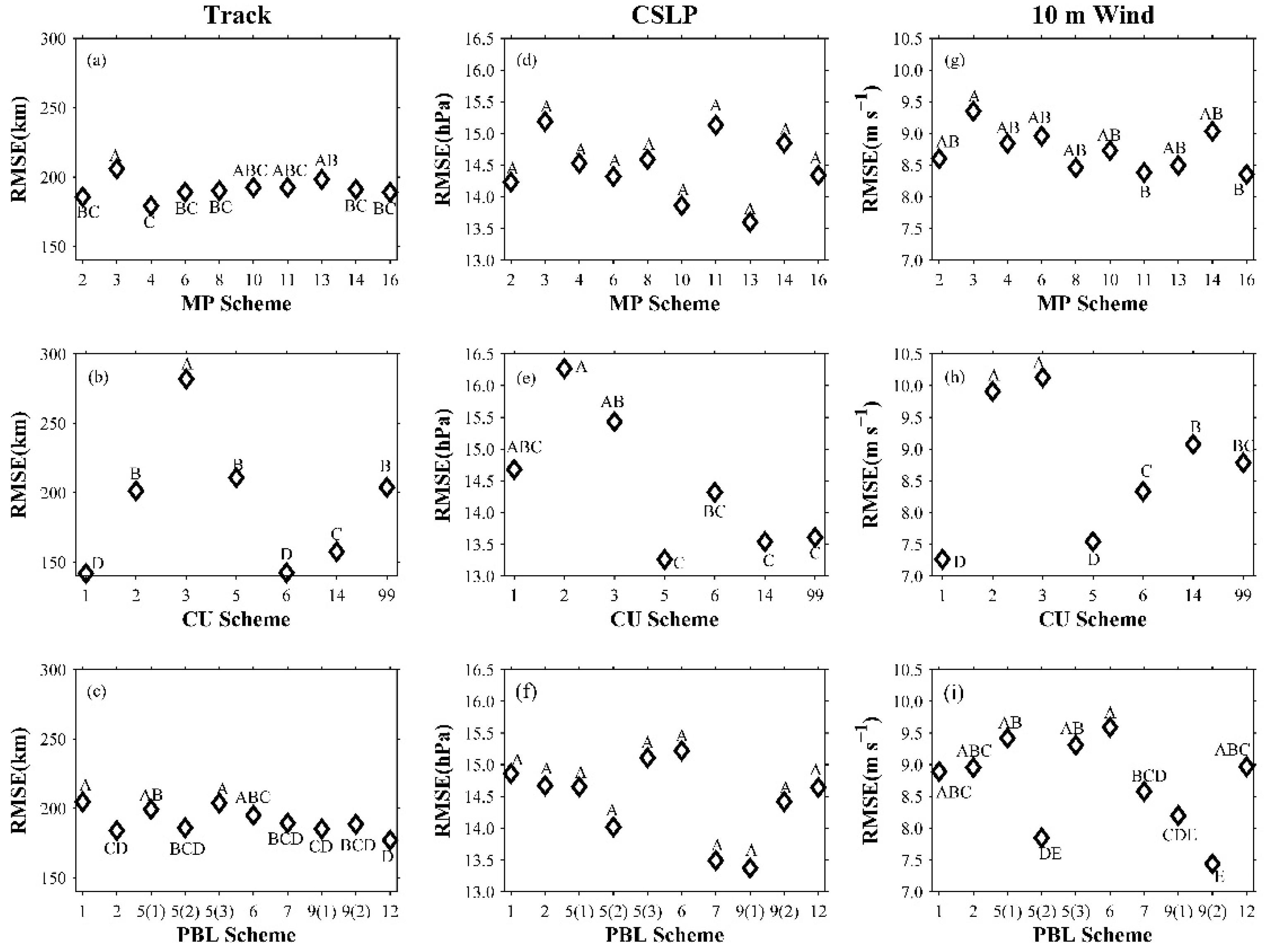
The first round of scheme evaluation results for track, CSLP, and 10-m wind using 140 samples are shown in Figure 2. The order of the population means at the 5% significance level was arranged as A > B > C > D > E. In each panel, if two schemes shared at least a letter in common, their population mean were not significantly different; otherwise, they were significantly different. For example, in Figure 2a, the MP schemes 3, 10, 11, and 13 all shared the letter “A”, and they were therefore not significantly different. In other words, their simulated population means were thought to be equal at this confidence level, and it was difficult to distinguish them from one another. On the other hand, the MP scheme 3 was assigned the letter “A”, while the MP scheme 16 was assigned the letters “BC”, which meant that these two MP schemes were significantly different, and that MP scheme 16 outperformed MP scheme 3. The reason was that the population mean of the errors of the sampled simulations, including the MP scheme 16, was lower than the population mean of the errors of the sampled simulations, including the MP scheme 3. Note also that transitivity did not exist amongst the MP schemes without significant differences due to the analysis results at a 5% significance level error. For instance, the MP scheme 10 assigned the letters “ABC” did not significantly differ from the MP scheme 3 assigned the letter “A” and the MP scheme 16 assigned the letters “BC”. However, the MP scheme 3 was significantly different from the MP scheme 16.
The MP schemes 3, 10, and 13 were assigned the letter “A”, but they were different. The reason was given as follows: The MP scheme 3 assigned the single letter “A” was classified to the worst group “A”; the MP scheme 13 assigned the letters “AB” meant that not only was it classified to the worst group “A”, but it was also classified to the middle group “B”. This made sense due to the 5% error that existed in the statistical analysis. The MP scheme 10 assigned the letters “ABC” meant that not only was it classified to the worst group “A” and the middle group “B”, but it was also classified to the best group ”C”. Obviously, it is clear that the MP scheme 3 only belonged to the worst group, and scheme 13 did not belong to the best group “C”. For the MP scheme 10 with the letters “ABC”, it could be classified to the worst group “A”, and also classified to the best group “C”, which was a vague group classification, and therefore, it was retained to the next round of scheme evaluations.
According to the above analyses, the worst MP scheme was defined as a scheme which was not significantly different from the MP scheme with the maximum population error, although it was significantly different from the MP scheme with the minimum population error. For instance, the MP schemes 3 and 13 in Figure 2a were considered the worst performing schemes but not the MP schemes 10 and 11, since they were not significantly different from the better MP scheme 4.
For multi-objective optimization, an MP scheme can only be deleted if it is considered as the worst performing scheme for all optimization variables. The MP scheme 3, assigned the letter “A”, was the common worst MP scheme for the three simulation variables (see Figure 2a,d,g) and should be deleted. However, the MP scheme 13 was only the worst-performing for track and CSLP, but not for 10-m wind, and therefore, could not be deleted at this point. Additionally, if no schemes were significantly different (e.g., Figure 2d), it meant that any of the schemes would produce consistent simulation errors, and therefore, deleting any of the schemes would not affect the accuracy of the ensemble. In a similar way, MP scheme 3, CU 3, and PBL schemes 1, 5(1), 5(3), and 6 were thought to be the common worst performing schemes and were deleted at the end of the first screening.
After the first round of screening, nine MP schemes, six CU schemes, and six PBL schemes remained. They are listed in Table S1 (Supplementary Information). Their least common multiple was 36; therefore, 72 samples were sampled from the three-dimensional physics dimensionalities using the QMC sampling method. Simulations and the Tukey’s test method were run as done previously. In all, four such evaluations were conducted and the Tukey’s test results for the second and third scheme evaluations are shown in the Supplementary Information, as Figures S1 and S2.
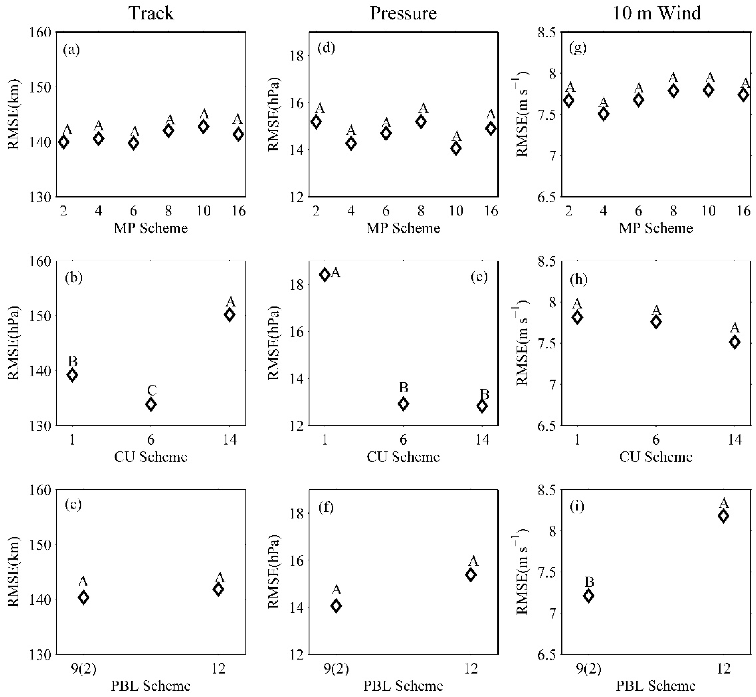
After the third round of screening, 6 MP schemes, 3 CU schemes, and 2 PBL schemes remained (see Table 3). Note that the number of full combinations for the remaining schemes was 36 (6 × 3 × 2). As it was acceptable to run all 36 combination simulations during the four rounds of scheme evaluations, the sampling method was not used and only the Tukey’s test was performed, with the results shown in Figure 3. At this point, no common worst scheme was left to be removed, and therefore, the multi-objective optimization was complete. The results in Figure 3 demonstrate that more than one optimal physics scheme exists for each variable. Therefore, determining a set of optimal scheme combinations for the three variables is difficult to achieve, and each variable has to be treated separately (a single-objective optimization). To achieve this purpose, the optimal ensemble for each variable was quantified, and the optimal scheme combination was determined from the ensemble member simulations. Finally, the optimal ensemble numbers for track, CSLP, and 10-m wind were 12 (6 × 1 × 2), 24 (6 × 2 × 2), and 18 (6 × 3 × 1), respectively.

3.2. Optimization Efficiency Analyses for Ensemble Simulations

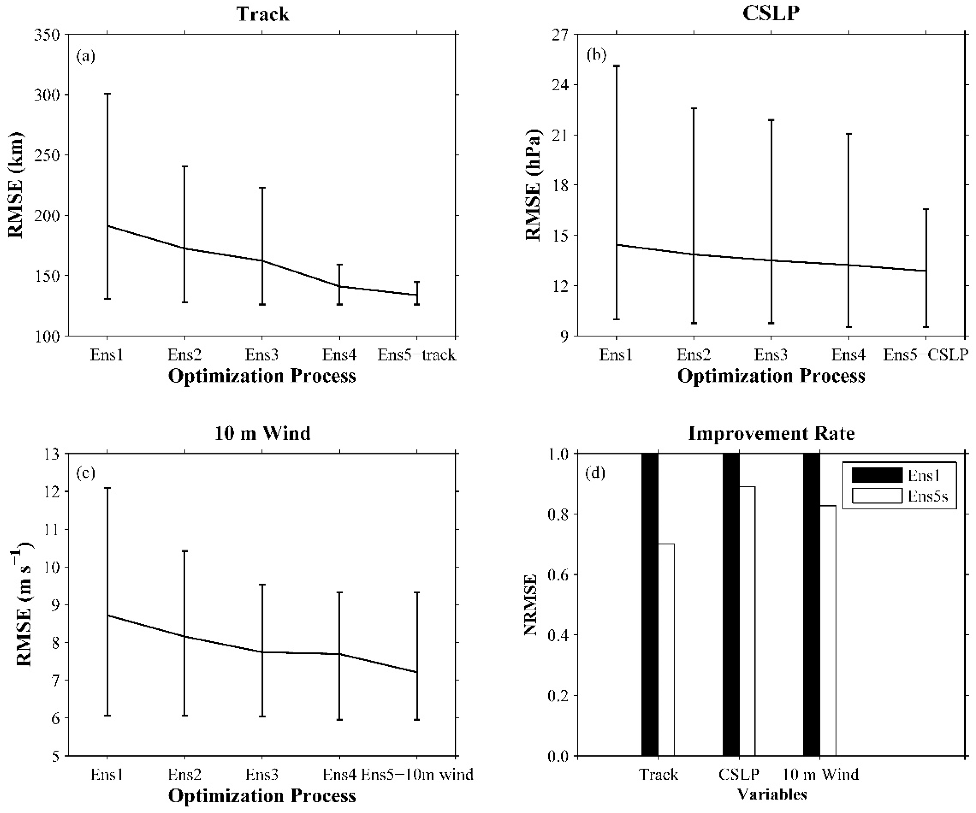
During the optimization process, four rounds of screening were conducted, and the sampled scheme combinations from each round could be viewed as an ensemble. The four ensembles were named Ens1, Ens2, Ens3, and Ens4 as the optimization order. Since the optimal ensembles for the track, CSLP, and 10-m wind were different, the optimal ensembles of track, CSLP, and 10-m wind were called as Ens5-track, Ens5-CSLP, and Ens5-10m wind, respectively. The three ensembles were also collectively named the Ens5s. Ultimately, the mean and variance of the five ensemble simulation errors for the three optimization variables were evaluated, and the error as a function of the ensemble for each variable is shown in Figure 4a–c. Both the mean and the variation range of the ensemble simulation errors gradually decreased for track, CSLP, and 10-m wind as the optimization progressed. Note that the error reduction from Ens1 to Ens5s was not due to fewer combinations being used. Since the scheme combinations for each round of screening were obtained by sampling rather than using full combinations, there were basically no common scheme combination elements for the different rounds of screening. Thus, the latter ensemble was not the subset of the previous ensemble, and therefore, the reduction of the ensemble number did not necessarily lead to the reduction in the simulation errors. Compared to the RMSE of Ens1, the RMSEs of the Ens5s for the three variables was normalized. The improvement percentages of the normalized RMSE for the Ens5s are shown in Figure 4d, and they are found to be maximum for the track simulation, and minimum for the CSLP. Based on the average values of the ensembles, the error decreases for the track, CSLP, and 10-m wind were 30.03%, 10.88%, and 17.32%, respectively. In addition, the error variance reduced from 169.51 to 18.55 km for track, from 15.12 to 7 hPa for CSLP, and from 6.03 m s−1 to 3.37 m s−1 for 10-m wind speed.
The results of the ensemble simulations for Ens1 and the Ens5s for the 15 single typhoon cases were also compared (Figure 5). This comparison revealed that the Ens5s improved all 15 typhoon track simulations compared to Ens1, and the overall improvement (i.e., error reduction) accounted for 30.03%. Compared to the track error of Ens1, the range of the Ens5-track error reduction varied from 6.11% for typhoon (14) to 67.17% for typhoon (11). For the CSLP simulations, four out of 15 typhoons had negative values (i.e., an increase in the error), with the maximum degradation occurring for typhoon (7) with −17.46%, whilst the other degradations were lower than 9%. However, the overall improvement for Ens5-CSLP compared to Ens1 was 10.88%. The occurrence of negative improvements was related to the cost function, which represented the average value of all the event simulation errors. If unequal weights were allocated to the simulation error of each event in the cost function, the negative improvement would disappear. There were also four negative improvements for the 10-m wind speed in the Ens5-10m wind simulations, with a maximum of approximately −25% for typhoons (4) and (13). However, these increases in the error only occured for the typhoons with lower simulation errors. Moreover, the number of typhoons with increased errors was much less than the typhoons which had a decrease in the simulation error. For all these reasons, there was no significant negative effect on the overall simulations from the use of the optimally determined schemes of the Ens5s.

3.3. Validation

The previous analysis (Figure 3) revealed that the Ens5s had 12, 24, and 18 scheme combinations for track, CSLP, and 10-m wind, respectively. For each variable, the optimal scheme combination was subsequently found by searching for the combination that yielded the minimum simulation error, where the optimal scheme combination for each variable is shown in Table 4. The Tiedtke CU scheme and the UW PBL scheme matched with the ETA SF scheme were the optimal schemes that were common for the simulations of track, CSLP, and 10-m wind. However, the optimal MP scheme for each variable was different. Specifically, the optimal MP schemes for track, CSLP, and 10-m wind were the Thompson, WSM5, and Lin schemes, respectively.
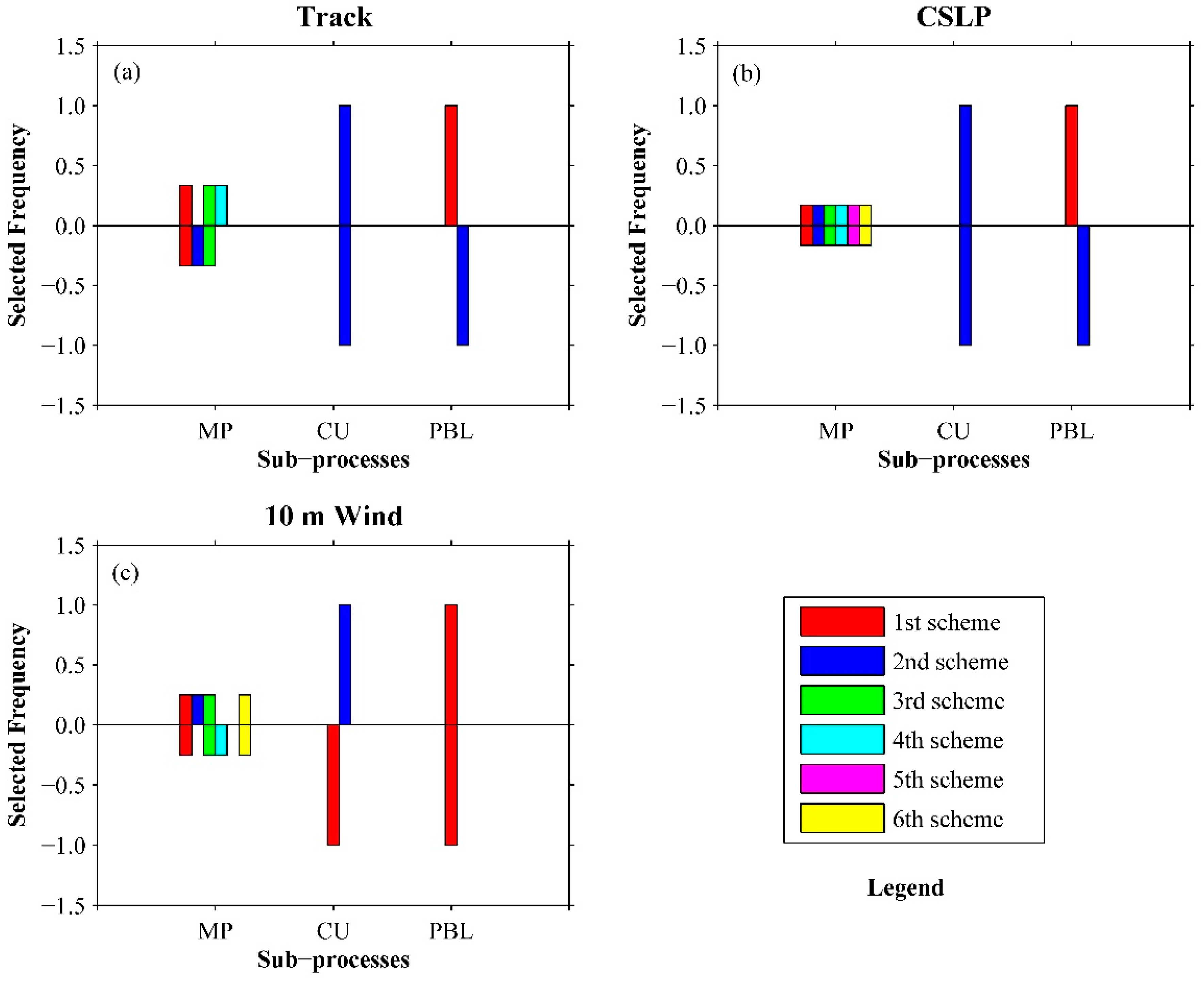
To assess the quality of the obtained optimal scheme combinations, the optimal ensemble (i.e., the Ens5s) of each variable was used to analyze the selected frequency of the optimal schemes. For each variable of the Ens5s, the scheme combinations falling below the 25th percentile of the RMSE were selected as the best members, and the scheme combinations ranking above the 75th percentile of the RMSE were selected as the worst members. The selected frequency of each scheme as the best (worst) member is then calculated by dividing the number of occurrences of the scheme by the total scheme number of the best (worst) members. The results for the frequency of the different schemes as the best and worst members are shown in Figure 6, as positive and negative bars, respectively. For clarity, the schemes for each physics module were named following their option order in Table 3. For example, the 6 MP schemes were called 1st, 2nd, …, and 6th MP scheme, from top to bottom. Similarly, the 3 CU schemes were called 1st, 2nd, and 3rd CU scheme, and the 2 PBL schemes were called the 1st and 2nd PBL scheme.
The results in Figure 6 show that the 2nd CU scheme (i.e., scheme 6) and 1st PBL scheme (i.e., scheme 9(2)) always behave as the best members for the three variables, implying that these two schemes present obvious advantages in obtaining optimal typhoon simulations compared to the other schemes in the same physics module. Since these two schemes systematically scored as the best members, the conclusion that they were selected as the optimal CU and PBL schemes (see Table 4) could be considered as very robust. On the other hand, our analysis revealed no highly recurrent MP scheme for any of the three variable simulations. The occurrence frequency of the MP schemes as the best members was similar for each variable, making the distinction of a single optimal MP scheme impossible.
The 2nd PBL scheme consistently scored as the worst member for track and CSLP, whilst the 1st CU scheme was consistently the worst member for the 10-m wind. These schemes should be deleted to avoid degradation in the quality of the simulations. Lastly, the three schemes that scored as the best and worst members were: the 2nd CU scheme for track and CSLP, and the 1st PBL scheme for 10-m wind. The reasons were as follows: The number of members in the Ens5-track, Ens5-CSLP, and Ens5-10m wind were 12, 24, and 18, respectively. The 2nd CU scheme and the 1st PBL scheme completely absorbed the 12 CU physics options of the Ens5-track and the 18 PBL physics options of the Ens5-10m wind, respectively. Therefore, the 2nd CU scheme and the 1st PBL scheme scored as the best and worst members for track, and 10-m wind, respectively. For the CU options of the 24 Ens5-CSLP members, half of the members used the 3rd CU scheme (i.e., scheme 14) and the other half used the 2nd CU scheme. All of the 2nd CU schemes lay in the best and worst members of the Ens5-CSLP, and half of them scored as the best members, while the other half scored as the worst members. It meant that the 2nd CU scheme had an equal probability of being divided into the best/worst performing members. If the 2nd CU scheme matched correctly with the other physic schemes, the typhoon CSLP simulation would be improved. Note that the discreteness was one of characters for the Ens5s. Here, the selected frequency/number of the optimal schemes in the best and worst members was used to verify the reasonableness of the optimal schemes obtained, which were also reasonable from the aspect of the ensemble.
Results from Figure 6 have demonstrated that the best and worst schemes can be clearly identified for the CU and PBL schemes, but not for the MP schemes. To analyze the effect of the different MP schemes on typhoon simulation, the results of six simulations was analyzed and compared. Each simulation ran under a set of different physics scheme combinations, using each of the 6 MP schemes, the optimal 2nd CU scheme, and the optimal 1st PBL schemes (see Table 3). These simulation results are shown in Table 5 in terms of the RMSE. The maximum difference values obtained amongst the six simulations for track, CSLP, and 10-m wind were 5.15 km, 0.89 hPa, and 1.14m s−1, respectively. These maximum difference values were small, accounting for only 4.08%, 9.32%, and 19.13% of each variable’s optimal simulation error. The six ensemble simulation errors ranged below the 28th, 13th, and 34th percentile of the Ens5s simulation errors for track, CSLP, and 10-m wind, respectively. Thus, these six scheme combinations could be classified as the best members, i.e., the variance range of the typhoon simulation errors was acceptable regardless of the MP scheme used, while fixing the optimal CU and PBL schemes.
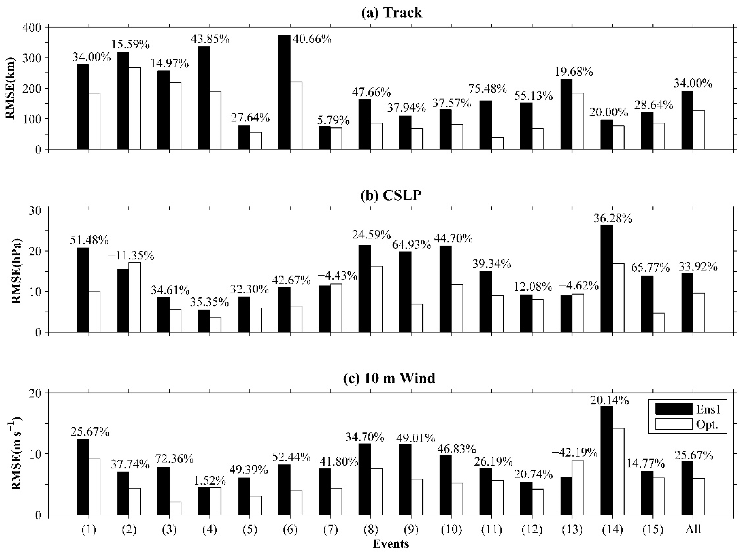
To further evaluate the effectiveness of the optimization method, typhoon simulations that were run with the optimal physics schemes (see Table 4) were compared with the averaged simulations of Ens1. The results are shown in Figure 7. The optimal scheme combination for the track simulations improved all the 15 typhoons track simulations compared to Ens1, with improvements (i.e., error reduction) ranging from 5.79% to 75.48%, and an overall improvement percentage of 34% for the track simulations. The averaged improvement percentage of the CSLP yielded by the optimal scheme combination was 33.92%, with the improvement ranging from 12.08% to 65.77%, except for three degraded typhoon simulations. Lastly, the overall improvement compared to Ens1 for the 10-m wind was 25.67%, with a minimum of 1.52% and a maximum of 52.44%, except for a degraded typhoon simulation. The improvement percentages of the three optimal simulations (Figure 7) were significantly higher than the percentages of the Ens5s (Figure 5), whilst the number of degraded typhoon simulations also decreased.

4. Discussion

4.1. Comparison to the Default Simulations

An in-depth analysis of the simulation results was conducted for two case studies, that is, for typhoons Vicente (201208) and Matmo (201410). For each case, two three-day WRF simulations were run. For the two case simulations, the designs of the domain and simulation, and the forcing data source, were the same as in the previous simulations. The first simulation used its optimal scheme combination setup for each variable (see Table 4), whilst the other simulation used the default scheme combination setup defined in Section 2.2. Except for the Dudhia shortwave, RRTM longwave, and Noah land-surface, the MP, CU, PBL, and SF schemes of the default scheme combination were different from the schemes of the optimal scheme combination. The observed track and intensity data was still obtained from the CMA-STI best track dataset for tropical cyclones over the Northwest Pacific Ocean. The typhoon tracks for Vicente (201208) and Matmo (201410) simulated with the default and optimal scheme combinations are shown in Figure 8. Overall, the improvement percentages for the track simulations of Vicente (201208) and Matmo (201410) were 20.62% and 58.32%, respectively. The optimal schemes WRF simulations were shown to be closer to the observations than the default simulations. The difference between the latter and the observations increased with time, whereas such differences were much more limited for simulations with the optimal schemes. A comparison of the track simulations between the default and the optimal schemes at the last time step (i.e., the 72nd hour) revealed that the optimal simulations improved the delayed prediction for typhoon Vicente (201208), and the early prediction of typhoon Matmo (201410). The early and delayed predictions would respectively yield the results of a false alarm and miss for the coast areas in which typhoons are about to make landfall. In addition, the remaining 13 typhoons track simulations were also analyzed, and the results demonstrated that the default simulations for three typhoon cases (i.e., typhoon events for 201209, 201307, and 201319) had early prediction, while the remaining 10 typhoon default simulations had delayed prediction. Finally, the range of the improvement percentages for the delay/early simulations of the 15 typhoons varied from 29% for typhoon Nanmadol (201111) to 76.65% for typhoon Vicente (201208), except for the five negative improvement typhoon simulations (i.e., −5.31% for typhoon Nesat (201117), −8.33% for typhoon Banyan (201120), −33.77% for typhoon Rammasun (201409), −0.73% for typhoon Kalmaegi (201415), and −1.64% for typhoon Linfa (201510)). Overall, the improvement percentage for the delay/early simulations of the 15 typhoons was 18.25%.
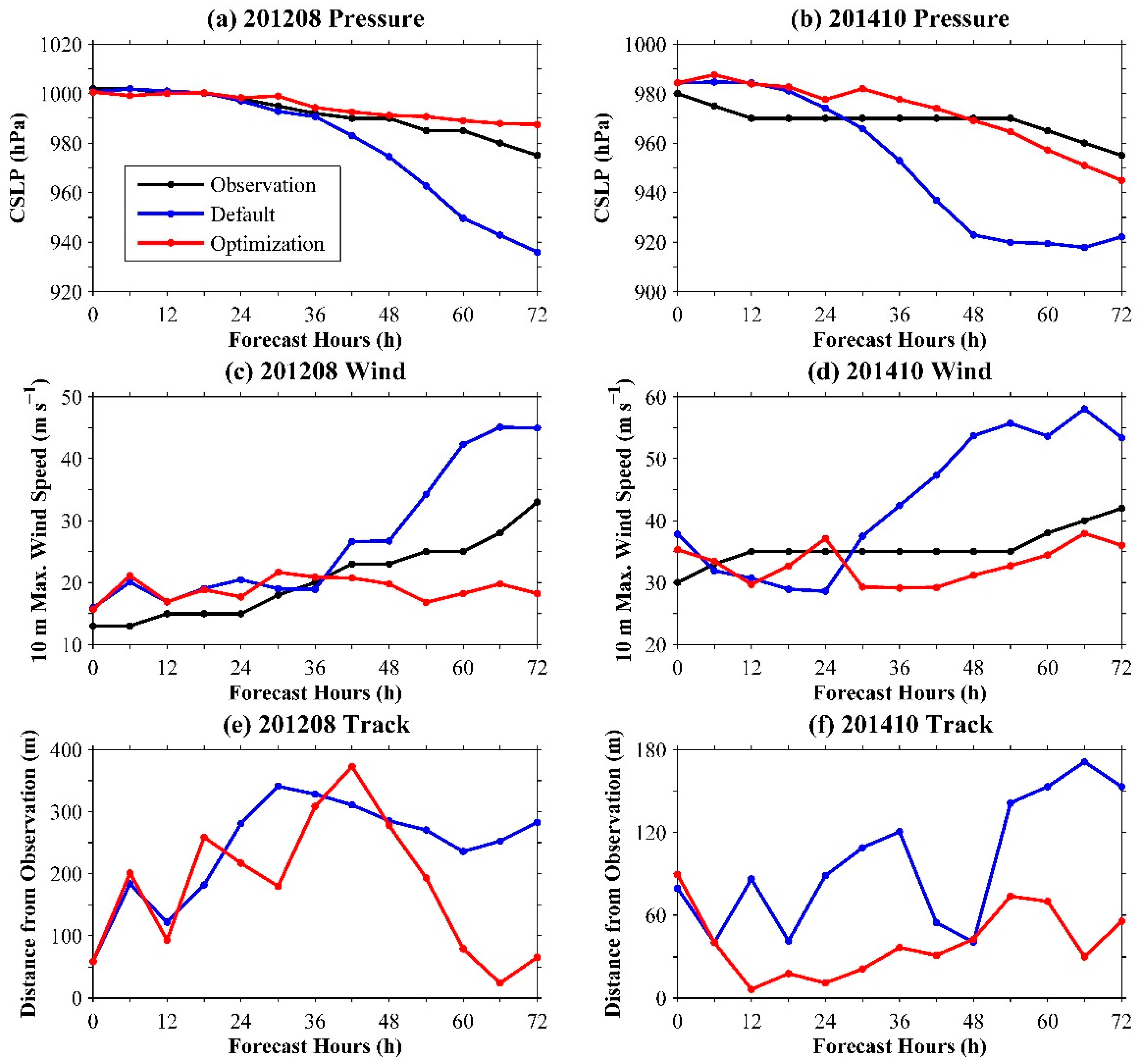
Besides the typhoons track, the simulations of typhoon intensity (i.e., CSLP and 10-m wind) were also compared. The results are shown in Figure 9a–d. Overall, the descending trend of the CSLP and ascending trend of the 10 m maximum wind speed were reproduced by both the default and optimal simulations, demonstrating that the typhoon intensity was reasonably well simulated by both schemes. However, the accuracy of simulation showed a great difference between the default and optimal cases. In the case of typhoon Vicente (201208), the default simulations of the CSLP and 10-m wind at the 36th hour exhibited large differences to the observations, and these biases further increased with time. The same situation occurred at the 32nd hour for typhoon Matmo (201410). These large biases were strongly reduced by the optimal simulations for both the CSLP and the 10-m wind, demonstrating the better accuracy yielded by this method. Specifically, the mean absolute error (MAE) of the three-day CSLP simulations with the optimal schemes for typhoons Vicente (201208) and Matmo (201410) decreased by 72.43% and 65.78%, respectively. For the 10-m wind speed, the MAE decrease using the optimal simulations for typhoon Vicente (201208) and Matmo (201410) was 22.06% and 61.76%, respectively.
The comparisons of track simulations using the default and optimal scheme combinations were also conducted. The results are shown in Figure 9e–f. The track simulations for typhoons Vicente (201208) and Matmo (201410) demonstrated that the default simulation error had a significantly ascending trend after the 24th h. The optimal simulation for typhoon Vicente (201208) decreased the track simulation error after 24 h, and the optimal simulation for typhoon Matmo (201410) always had a low error compared to the default simulation. The track conclusions could explain the reasonability of the previous CSLP and wind simulations. Overall, these large error reductions further demonstrated that the optimal scheme combination was more suitable for the typhoon simulations than the default scheme combination.
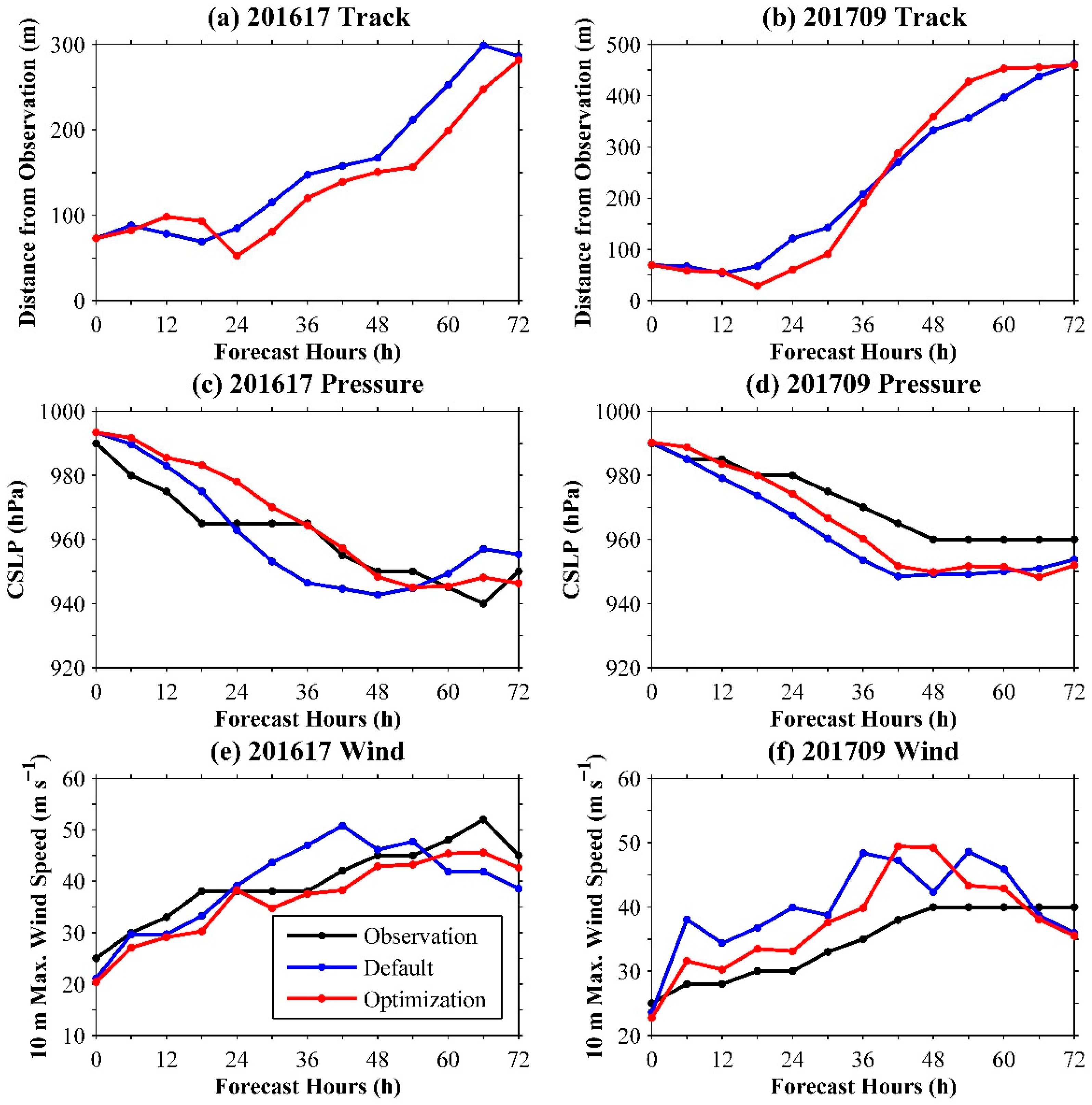
Additionally, the two independent typhoon events from 2016 to 2017 were also simulated to demonstrate the superiority of the optimal scheme combinations. The two cases were typhoon Megi (201617) and typhoon Nesat (201709), and their simulation periods were 3 days. For each three-day typhoon simulation, the designs of the domain and simulation, and the forcing data source, were the same as the previous optimization simulations, except for the schemes of the MP, CU, and PBL physics. One simulation used the default scheme combination and the other simulation used the optimal scheme combination. The comparison results of the track, CSLP, and 10-m wind are shown in Figure 10. For the track simulations, the simulation with the optimal scheme combination had a lower error than the default scheme combination for typhoon Megi (201617), and there was little improvement for typhoon Nesat (201709). The overall improvement percentages for the track simulations of Megi (201617) and Nesat (201709) were 12.64% and −0.38%, respectively. For the CSLP simulations, the simulation with the optimal scheme combination was closer to the observation than to the default scheme combination. The overall improvement percentages for the CSLP simulations of Megi (201617) and Nesat (201709) were 16.49% and 23.82%, respectively. The same situation occured in the 10-m wind simulations. The improvement percentages for the 10-m wind simulations of Megi (201617) and Nesat (201709) were 33.19% and 30.39%, respectively. These results further demonstrated the superiority of the optimal scheme combination on the typhoon simulations, and therefore, the optimal scheme combination obtained was thought to be reasonable.

4.2. Comparison of the Optimal Configuration with the Literature

From the previous analyses, the optimal MP, CU, and PBL schemes for typhoon simulations over the Northwest Pacific Ocean were determined. These were the Thompson MP scheme, Tiedtke CU scheme, and the UW PBL scheme matched with the ETA SF scheme for typhoon track simulation. The WSM5 MP Scheme, Tiedtke CU scheme, and the UW PBL scheme matched with the ETA SF scheme for typhoon CSLP simulation. The Lin MP scheme, Tiedtke CU scheme, and the UW PBL scheme matched with ETA SF scheme for typhoon 10 m maximum wind speed simulation.
There are some existing studies on the sensitivities of physics schemes to the typhoon simulations, although the optimal CU and PBL schemes have fewer considerations in the previous studies. Therefore, there is no evidence to prove that our optimal CU and PBL schemes are superior to the optimal schemes of other studies for typhoon simulation. However, our optimal MP schemes, including the Thompson, WSM5, and Lin MP schemes, have been commonly analyzed. Therefore, there can only be a comparison of the difference in the optimal MP results for typhoon simulations between our study and other studies. Chandrasekar et al. [21] found that the Thompson MP scheme outperformed the WSM5 MP scheme and the Lin MP scheme for typhoon track simulation; and that the Lin MP scheme outperformed the WSM5 MP scheme and the Thompson MP scheme for 10-m wind simulation, which was completely consistent with our conclusions. The superiorities of the three MP schemes to other MP schemes on typhoon simulations were also demonstrated in studies performed by Raju et al. [20] and Srinivas et al. [26]. Those examples demonstrated that our optimal MP schemes were reasonable for typhoon simulations. In addition, the default scheme combination (i.e., the WSM6 MP scheme, the KF CU scheme, and the YSU BPL scheme) has not been recognized to be optimal in some studies on scheme comparisons, such as Raju et al. [20]. We also found that the default scheme combination did not perform very well compared to the optimal scheme combinations.

4.3. Physical Interpretation and Verification of the Optimal Schemes

For the description of the MP process, the Thompson scheme was developed on the basis of the WSM6 scheme. Besides that, the Thompson scheme not only increased the ice number concentration prediction, but it also improved the rain distribution function from the empirical relationship formula to the function of the cloud–water mixing ratio [59]. The accurate rain simulation amount will release the reasonable latent heat, which can effectively heat the middle and upper atmosphere, such that the central pressure continues to reduce, thereby promoting the reasonable development of the typhoon. The Tiedtke cumulus scheme uses a mass flux scheme to describe three types of convection: penetrative convection, shallow convection, and midlevel convection. The KF scheme is a simple cloud model, including the updraft and downdraft. The Tiedtke scheme describes a more complex convection process than the KF scheme, and therefore, has a higher typhoon forecast accuracy [60,61]. For the description of the PBL process, the UW scheme applies a local turbulence kinetic energy-based closure, whilst the YSU scheme is a first-order nonlocal closure model. Given that the steeper slope relationship between the evaporation and wind speed exists in the UW scheme, the UW scheme enhances the typhoon wind simulation compared to the YSU scheme [62,63], which makes the simulated 10-m wind closer to the observation.

5. Conclusions

In this study, a Tukey-based optimization method was proposed to determine the optimal scheme combination for the simulation of a typhoon’s track and intensity (CSLP and 10-m wind), without running all the possible scheme combinations. For this purpose, three-day simulations of 15 typhoons that occurred over the Northwest Pacific Ocean between 2011 and 2015 were run under different configurations. All the schemes of the WRF sensitive physics modules (i.e., MP, CU, and PBL) in typhoon simulation were analyzed, whilst other physics schemes were fixed.
Four rounds of screening were conducted to minimize the number of scheme combinations, which was 140 before the first screening (Ens1), and 12~24 after the fourth screening (Ens5s). The simulation results of the samples (i.e., the sampled scheme combinations) for each round were averaged to assess the effectiveness of each scheme in the samples using the Tukey’s test method. This analysis revealed that the RMSE between the (track, CSLP, and 10-m wind) simulations and the observations was considerably reduced for the Ens5s compared to Ens1. Furthermore, the 284 simulations were run across four rounds of screenings, which accounted for 40% of all simulations with 700 possible scheme combinations (i.e., 10 MP × 7 CU × 10 PBL), which makes the Tukey-based optimization method efficient. In each round of the Tukey’s test analysis, the main effect (i.e., population mean) of each single scheme was only evaluated to delete the worst-performing scheme. However, the mutual interaction between the different physics schemes was not taken into account due to the complexity.
As the screenings progressed, not only did the mean error of each ensemble simulation decrease, but also the error variance decreased, which demonstrated that it was reasonable to exclude the worst-performing schemes using the Tukey’s test in each round of screening. Compared to the mean simulation error of Ens1, the errors of the Ens5-track, Ens5-CSLP, and Ens5-10-m wind decreased by 30.03%, 10.88%, and 17.32%, respectively. A detailed analysis of the 15 typhoon simulations of Ens1 and the Ens5s was also conducted. All the track simulations, and most of the CSLP and 10-m wind simulations of the Ens5s, were found to have improved compared to Ens1. The few cases of CSLP and 10-m wind simulations which are degraded corresponded to typhoons with a small original error, and these degradations were found not to be significant.
Consistent optimal CU and PBL schemes (i.e., the Tiedtke CU scheme, UW PBL scheme matched with the ETA SF scheme) for the three variable simulations were found, while the optimal MP schemes for the three variable simulations were different. In particular, the optimal CU and PBL schemes yielded simulations that were all within the best error range of the Ens5s for the three variables. This demonstrated the robustness of this conclusion for the optimal CU and PBL schemes. While no consistent optimal MP schemes were found, further tests demonstrated that any of the six MP schemes were combined with the optimal CU and PBL schemes, causing maximum variations of 4.08%, 9.32%, and 19.13% in the optimal simulation errors for the track, CSLP, and 10-m wind, respectively. Therefore, it is acceptable that any of the six MP schemes can used as the optimal MP scheme. Additionally, with these optimal schemes, the simulation error reduction in Ens1 for track, CSLP, and 10-m wind was 34%, 33.92%, and 25.67%, respectively.
Case studies for two typhoons were then carried out by comparing the simulation results for the default scheme combination and the optimal scheme combination. This final series of tests showed significant improvements. The intensity (CSLP and 10-m wind) simulations saw the largest biases occurring at the 32nd h of the default case and disappearing for the optimal case. The MAE of the overall simulations for the CSLP (10-m maximum wind speed) of typhoons Vicente (201208) and Matmo (201410) was 72.43% (22.06%) and 65.78% (61.76%), respectively. In particular, the delayed track prediction for typhoon Vicente (201208), and the early track prediction for typhoon Matmo (201410) at the last time step of the simulation were strongly improved when using the optimal schemes. This implied that the simulation for the typhoons landing time would become more accurate under optimal simulations in the future, which may limit the economic and human losses for countries hit by the typhoons. In addition, the two additional typhoon cases were simulated using the WRF model with the default and optimal scheme combination. The results further demonstrated the superiority of the optimal scheme combination on the typhoon simulations, and therefore, the optimal scheme combination that was obtained was thought to be reasonable.
Some limitations exist in our approach. For example, the simulation included all 15 typhoons that occurred over the ocean without considering typhoon landing, which was done to avoid the influence of complex land surface parameters (e.g., terrain and surface roughness) on the simulation. In addition, precipitation simulations were also not evaluated due to the deficiency of accurate precipitation data in the ocean. Lastly, neither dynamic initialization nor data assimilation was used to improve the accuracy of the initial and boundary values for the typhoon simulations. Therefore, future studies could be focused on the optimization of the WRF schemes using more accurate initial and boundary data, and the assessment of the WRF optimal schemes for landing typhoon simulations. In spite of these limitations, the decreased computational cost and large improvements in the quality of the typhoons track and intensity simulations make the Tukey-based optimization method a very effective and efficient tool for the crucial forecasting of typhoons.

Supplementary Materials

The following are available online at https://www.mdpi.com/2073-4433/10/5/233/s1, Figure S1: Tukey’s test results of the three physics modules for the (a)–(c) track, (d)–(f) central sea level pressure (CSLP), and (g)–(i) 10 m maximum wind speed (10-m wind) at the second round of screening, Figure S2: Tukey’s test results of the three physics schemes for the track, CSLP, and 10-m wind at the third round of screening, Table S1: Selected physics parameterization schemes at the end of the first round of screening, using the Tukey-based optimization method.

Author Contributions

Data curation, Z.D. and C.S.; Methodology, Z.D., W.G., and Y.G.; Formal analysis, Z.D. and W.G.; Writing—Original Draft preparation, Z.D.; Supervision, Z.D. and Q.D.

Funding

This research was supported by the National Basic Research Program of China (2015CB953703), the State Key Laboratory of Earth Surface Processes and Resource Ecology (2017-KF-03), and the National Natural Science Foundation of China (41305052).

Acknowledgments

Special thanks to the group of Jing Xu at the State Key Laboratory of Severe Weather and the Chinese Academy of Meteorological Sciences for offering help with the typhoon simulations and data collection. Typhoon data are available online at http://tcdata.typhoon.org.cn/zjljsjj_sm.html.

Conflicts of Interest

The authors declare no conflict of interest.

References

  1. Skamarock, W.C.; Klemp, J.B.; Dudhia, J.; Gill, D.O.; Barker, D.M.; Duda, M.G.; Huang, X.; Wang, W.; Powers, J.G. A Description of the Advanced Research WRF Version 3. NCAR Technical Note, NCAR/TN-475+STR. 2008. Available online: https://opensky.ucar.edu/islandora/object/technotes%3A500/datastream/PDF/view (accessed on 8 June 2008).
  2. Wang, Y. On the bogussing of tropical cyclones in numerical models: The influence of vertical structure. Meteor. Atmos. Phys. 1998, 65, 153–170. [Google Scholar] [CrossRef]
  3. Davidson, N.E.; Weber, H.C. The BMRC High-Resolution Tropical Cyclone Prediction System: TC-LAPS. Mon. Wea. Rev. 2000, 128, 1245–1265. [Google Scholar] [CrossRef]
  4. Ma, S.; Qu, A.; Wang, Y. The performance of the new tropical cyclone track prediction system of the China National Meteorological Center. Meteor. Atmos. Phys. 2007, 97, 29–39. [Google Scholar] [CrossRef]
  5. Kwon, I.H.; Cheong, H.B. Tropical cyclone initialization with a spherical high-order filter and an idealized three-dimensional bogus vortex. Mon. Wea. Rev. 2010, 138, 1344–1367. [Google Scholar] [CrossRef]
  6. Zou, X.; Xiao, Q. Studies on the initialization and simulation of a mature hurricane using a variational bogus data assimilation scheme. J. Atmos. Sci. 2000, 57, 836–860. [Google Scholar] [CrossRef]
  7. Zhang, X.; Xiao, Q.; Fitzpatrick, P.J. The impact of multisatellite data on the initialization and simulation of Hurricane Lili’s (2002) rapid weakening phase. Mon. Wea. Rev. 2007, 135, 526–548. [Google Scholar] [CrossRef]
  8. Liu, Y.; Zhang, W. Improved hurricane forecasting from a variational bogus and ozone data assimilation (BODA) scheme: Case study. Meteorol. Atmos. Phys. 2016, 128, 1–18. [Google Scholar] [CrossRef]
  9. Lu, X.; Wang, X.; Li, Y.; Tong, M.; Ma, X. GSI-based, continuously cycled, dual-resolution hybrid- variational data assimilation system for HWRF: System description and experiments with Edouard (2014). Mon. Wea. Rev. 2017, 145, 4877–4898. [Google Scholar] [CrossRef]
  10. Lin, K.; Yang, S.; Chen, S. Reducing TC position uncertainty in an ensemble data assimilation and prediction system: A case study of Typhoon Fanapi (2010). Weather Forecast 2018, 33, 561–582. [Google Scholar] [CrossRef]
  11. Van Nguyen, H.; Chen, Y.L. High-resolution initialization and simulations of Typhoon Morakot (2009). Mon. Wea. Rev. 2011, 139, 1463–1491. [Google Scholar] [CrossRef]
  12. Cha, D.H.; Wang, Y. A dynamical initialization scheme for real-time forecasts of tropical cyclones using the WRF Model. Mon. Wea. Rev. 2013, 141, 964–986. [Google Scholar] [CrossRef]
  13. Xu, J.; Wang, Y. A statistical analysis on the dependence of tropical cyclone intensification rate on the storm intensity and size in the North Atlantic. Weather Forecast 2015, 30, 692–701. [Google Scholar] [CrossRef]
  14. Donelan, M.A.; Haus, B.K.; Reul, N.; Plant, W.J.; Stiassnie, M.; Graber, H.C.; Brown, O.B.; Saltzman, E.S. On the limiting aerodynamic roughness of the ocean in very strong winds. Geophys. Res. Lett. 2004, 31, L18306. [Google Scholar] [CrossRef]
  15. Zeng, Z.; Wang, Y.; Duan, Y.; Chen, L.; Gao, Z. On sea surface roughness parameterization and its effect on tropical cyclone structure and intensity. Adv. Atmos. Sci. 2010, 27, 337–355. [Google Scholar] [CrossRef]
  16. Kim, T. Evaluation of wave-dependent surface roughness parameterization using a coupled atmosphere-wave model. American Geophysical Union, Ocean Sciences Meeting 2016, abstract# A54C-2733. Available online: http://adsabs.harvard.edu/abs/2016AGUOS.A54C2733K (accessed on 21 March 2019).
  17. Ma, L.M.; Tan, Z.M. Improving the behavior of the cumulus parameterization for tropical cyclone prediction: Convection trigger. Atmos. Res. 2009, 92, 190–211. [Google Scholar] [CrossRef]
  18. Emanuel, K.; Desautels, C.; Holloway, C.; Korty, R. Environmental control of tropical cyclone intensity. J. Atmos. Sci. 2004, 61, 843–858. [Google Scholar] [CrossRef]
  19. Davis, C.; Wang, W.; Chen, S.S.; Chen, Y.; Corbosiero, K.; Demaria, M.; Dudhia, J.; Holland, G.; Klemp, J.; Michalakes, J.; et al. Prediction of landfalling hurricanes with the advanced hurricane WRF model. Mon. Wea. Rev. 2008, 136, 1990–2005. [Google Scholar] [CrossRef]
  20. Raju, P.V.S.; Potty, J.; Mohanty, U.C. Sensitivity of physical parameterizations on prediction of tropical cyclone Nargis over the Bay of Bengal using WRF model. Meteorol. Atmos. Phys. 2011, 113, 125–137. [Google Scholar] [CrossRef]
  21. Chandrasekar, R.; Balaji, C. Sensitivity of tropical cyclone Jal simulations to physics parameterizations. J. Earth Syst. Sci. 2012, 121, 923–946. [Google Scholar] [CrossRef]
  22. Osuri, K.K.; Mohanty, U.C.; Routray, A.; Kulkarni, M.A.; Mohapatra, M. Customization of WRF-ARW model with physical parameterization schemes for the simulation of tropical cyclones over North Indian Ocean. Nat. Hazards 2012, 63, 1337–1359. [Google Scholar] [CrossRef]
  23. Nasrollahi, N.; Aghakouchak, A.; Li, J.; Gao, X.; Hsu, K.; Sorooshian, S. Assessing the impacts of different WRF precipitation physics in hurricane simulations. Weather Forecast 2012, 27, 1003–1016. [Google Scholar] [CrossRef]
  24. Efstathiou, G.A.; Zoumakis, N.M.; Melas, D.; Lolis, C.J.; Kassomenos, P. Sensitivity of WRF to boundary layer parameterizations in simulating a heavy rainfall event using different microphysical schemes. Effect on large-scale processes. Atmos. Res. 2013, 132–133, 125–143. [Google Scholar] [CrossRef]
  25. Li, X. Sensitivity of WRF simulated typhoon track and intensity over the Northwest Pacific Ocean to cumulus schemes. Sci. China Earth Sci. 2013, 56, 270–281. [Google Scholar] [CrossRef]
  26. Srinivas, C.V.; Rao, D.B.; Yesubabu, V.; Baskaran, R.; Venkatraman, B. Tropical cyclone predictions over the Bay of Bengal using the high-resolution Advanced Research Weather Research and Forecasting (ARW) model. Q. J. Roy. Meteor. Soc. 2013, 139, 1810–1825. [Google Scholar] [CrossRef]
  27. Kanase, R.D.; Salvekar, P.S. Impact of physical parameterization schemes on track and intensity of severe cyclonic storms in Bay of Bengal. Meteorol. Atmos. Phys. 2015, 127, 537–559. [Google Scholar] [CrossRef]
  28. Chen, S.; Qian, Y.K.; Peng, S. Effects of various combinations of boundary layer schemes and microphysics schemes on the track forecasts of tropical cyclones over the South China Sea. Nat. Hazards 2015, 78, 61–74. [Google Scholar] [CrossRef] [Green Version]
  29. Islam, T.; Srivastava, P.K.; Rico-Ramirez, M.A.; Dai, Q.; Gupta, M.; Singh, S.K. Tracking a tropical cyclone through WRF–ARW simulation and sensitivity of model physics. Nat. Hazards 2015, 76, 1473–1495. [Google Scholar] [CrossRef]
  30. Zhang, G.; Chen, F.; Gan, Y. Assessing uncertainties in the Noah-MP ensemble simulations of a cropland site during the Tibet Joint International Cooperation program field campaign. J. Geophys. Res. Atmos. 2016, 121, 9576–9596. [Google Scholar] [CrossRef]
  31. Ying, M.; Zhang, W.; Yu, H.; Lu, X.; Feng, J.; Fan, Y.; Zhu, Y.; Chen, D. An overview of the China Meteorological Administration tropical cyclone database. J. Atmos. Ocean. Techn. 2014, 31, 287–301. [Google Scholar] [CrossRef]
  32. WRF User’s Guide. User’s Guide for the Advanced Research WRF (ARW) Modeling System Version 3.6. Available online: http://www2.mmm.ucar.edu/wrf/users/docs/user_guide_V3/ARWUsersGuideV3.pdf (accessed on 18 September 2014).
  33. Xu, X.; Lu, C.; Xu, H.; Chen, L. A possible mechanism responsible for exceptional rainfall over Taiwan from Typhoon Morakot. Atmos. Sci. Lett. 2011, 12, 294–299. [Google Scholar] [CrossRef] [Green Version]
  34. Liou, K.N.; Chou, M.D. Recent Progress in Atmospheric Science: Applications to the Asia-Pacific Region; World Scientific Publishing: Paleo Faliro, Greece, 2008; p. 486. [Google Scholar]
  35. NCEP. NCEP FNL Operational Model Global Tropospheric Analyses, Continuing from July 1999. Available online: https://doi.org/10.5065/D6M043C6 (accessed on 21 March 2019).
  36. Hong, S.Y.; Lim, J.O.J. The WRF single-moment 6-class microphysics scheme (WSM6). J. Korean Meteor. Soc. 2006, 42, 129–151. [Google Scholar]
  37. Kain, J.S. The Kain-Fritsch convective parameterization: An update. J. Appl. Meteor. Clim. 2004, 43, 170–181. [Google Scholar] [CrossRef]
  38. Hong, S.Y.; Noh, Y.; Dudhia, J. A new vertical diffusion package with an explicit treatment of entrainment processes. Mon. Wea. Rev. 2006, 134, 2318–2341. [Google Scholar] [CrossRef]
  39. Jiménez, P.A.; Dudhia, J.; González-Rouco, J.F.; Navarro, J.; Montávez, J.P.; García-Bustamante, E. A revised scheme for the WRF surface layer formulation. Mon. Wea. Rev. 2012, 140, 898–918. [Google Scholar] [CrossRef]
  40. Dudhia, J. Numerical study of convection observed during the winter monsoon experiment using a mesoscale two-dimensional model. J. Atmos. Sci. 1989, 46, 3077–3107. [Google Scholar] [CrossRef]
  41. Mlawer, E.J.; Taubman, S.J.; Brown, P.D.; Iacono, M.J.; Clough, S.A. Radiative transfer for inhomogeneous atmospheres: RRTM, a validated correlated-k model for the longwave. J. Geophys. Res. 1997, 102, 16663–16682. [Google Scholar] [CrossRef] [Green Version]
  42. Chen, F.; Dudhia, J. Coupling an advanced land surface–hydrology model with the Penn State–NCAR MM5 modeling system. Part I: Model implementation and sensitivity. Mon. Wea. Rev. 2001, 129, 569–585. [Google Scholar] [CrossRef]
  43. Milbrandt, J.A.; Yau, M.K. A multimoment bulk microphysics parameterization. Part I: Analysis of the role of the spectral shape parameter. J. Atmos. Sci. 2005, 62, 3051–3064. [Google Scholar] [CrossRef]
  44. Khain, A.; Pokrovsky, A.; Pinsky, M. Simulation of effects of atmospheric aerosols on deep turbulent convective clouds using a spectral microphysics mixed-phase cumulus cloud model. Part I: Model description and possible applications. J. Atmos. Sci. 2004, 61, 2963–2982. [Google Scholar] [CrossRef]
  45. Khain, A.; Lynn, B.; Dudhia, J. Aerosol effects on intensity of landfalling hurricanes as seen from simulations with the WRF model with spectral bin microphysics. J. Atmos. Sci. 2010, 67, 365–384. [Google Scholar] [CrossRef]
  46. Zhang, G.J.; McFarlane, N.A. Sensitivity of climate simulations to the parameterization of cumulus convection in the Canadian Climate Centre general circulation model. Atmos. Ocean. 1995, 33, 407–446. [Google Scholar] [CrossRef]
  47. Angevine, W.M.; Jiang, H.; Mauritsen, T. Performance of an Eddy Diffusivity-Mass Flux Scheme for Shallow Cumulus Boundary Layers. Mon. Wea. Rev. 2010, 138, 2895–2912. [Google Scholar] [CrossRef]
  48. Pan, H.L.; Wu, W.S. Implementing a Mass Flux Convective Parameterization Package for the NMC Medium-Range Forecast Model. NMC Office Note 409. 1995. Available online: https://repository.library.noaa.gov/view/noaa/11429 (accessed on 21 March 2019).
  49. Hong, S.Y.; Pan, H.L. Nonlocal boundary layer vertical diffusion in a Medium-Range Forecast model. Mon. Wea. Rev. 1996, 124, 2322–2339. [Google Scholar] [CrossRef]
  50. Kessler, E. On the distribution and continuity of water substance in atmospheric circulations. Meteor. Monogr. 1969, 32, 1–84. [Google Scholar]
  51. Rogers, E.; Black, T.; Ferrier, B.; Lin, Y.; Parrish, D.; DiMego, G. Changes to the NCEP Meso Eta Analysis and Forecast System: Increase in Resolution, New Cloud Microphysics, Modified Precipitation Assimilation, Modified 3DVAR Analysis; NWS Technical Procedures Bulletin 488; NOAA/NWS: Silver Spring, MA, USA, 2001.
  52. Tao, W.K.; Simpson, J.; McCumber, M. An ice-water saturation adjustment. Mon. Wea. Rev. 1989, 117, 231–235. [Google Scholar] [CrossRef]
  53. Mansell, E.R.; Ziegler, C.L.; Bruning, E.C. Simulated Electrification of a Small Thunderstorm with Two-Moment Bulk Microphysics. J. Atmos. Sci. 2010, 67, 171–194. [Google Scholar] [CrossRef] [Green Version]
  54. Grell, G.A.; Dévényi, D. A generalized approach to parameterizing convection combining ensemble and data assimilation techniques. Geophys. Res. Lett. 2002, 29, 381–384. [Google Scholar] [CrossRef]
  55. Tukey, J.W. Comparing individual means in the analysis of variance. Biometrics 1949, 5, 99–114. [Google Scholar] [CrossRef]
  56. Hou, Z.; Huang, M.; Leung, L.R.; Lin, G.; Ricciuto, D.M. Sensitivity of surface flux simulations to hydrologic parameters based on an uncertainty quantification framework applied to the Community Land Model. J. Geophys. Res. 2012, 117, D15108. [Google Scholar] [CrossRef]
  57. Wang, C.; Duan, Q.; Gong, W.; Ye, A.; Di, Z.; Miao, C. An evaluation of adaptive surrogate modeling based optimization with two benchmark problems. Environ. Modell. Softw. 2014, 60, 167–179. [Google Scholar] [CrossRef] [Green Version]
  58. Gong, W.; Duan, Q.; Li, J.; Wang, C.; Di, Z.; Ye, A.; Miao, C.; Dai, Y. An intercomparison of sampling methods for uncertainty quantification of environmental dynamic models. J. Environ. Inf. 2016, 28, 11–24. [Google Scholar]
  59. Wang, Y.; Zhou, L.; Hamilton, K. Effect of Convective entrainment/detrainment on the simulation of the tropical precipitation diurnal cycle*. Mon. Weather Rev. 2007, 135, 567–585. [Google Scholar] [CrossRef]
  60. Yang, W.; Feng, W.; Li, X. Impacts of microphysical processes and cumulus parameterization schemes on simulated rainfall in Autumn over the Hainan Island. Torr. Rain Disas. 2017, 36, 8–17. [Google Scholar]
  61. Que, L.; Que, W.; Feng, J. Intercomparison of different physics schemes in the WRF model over the Asian summer monsoon region. Atmos. Oceanic Sci. Lett. 2016, 9, 169–177. [Google Scholar] [CrossRef]
  62. Huang, W.; Shen, X.; Wang, W.; Huang, W. Comparison of the thermal and dynamic structural characteristics in boundary layer with different boundary layer parameterization. Chin. J. Geophys. 2015, 57, 1399–1414. [Google Scholar]
  63. Qian, Y.; Yan, H.; Berg, L.K.; Hagos, S.; Feng, Z.; Yang, B.; Huang, M. Assessing impacts of PBL and surface layer schemes in simulating the surface–atmosphere interactions and precipitation over the tropical ocean using observations from AMIE/DYNAMO. J. Climate 2016, 29, 8191–8210. [Google Scholar] [CrossRef]
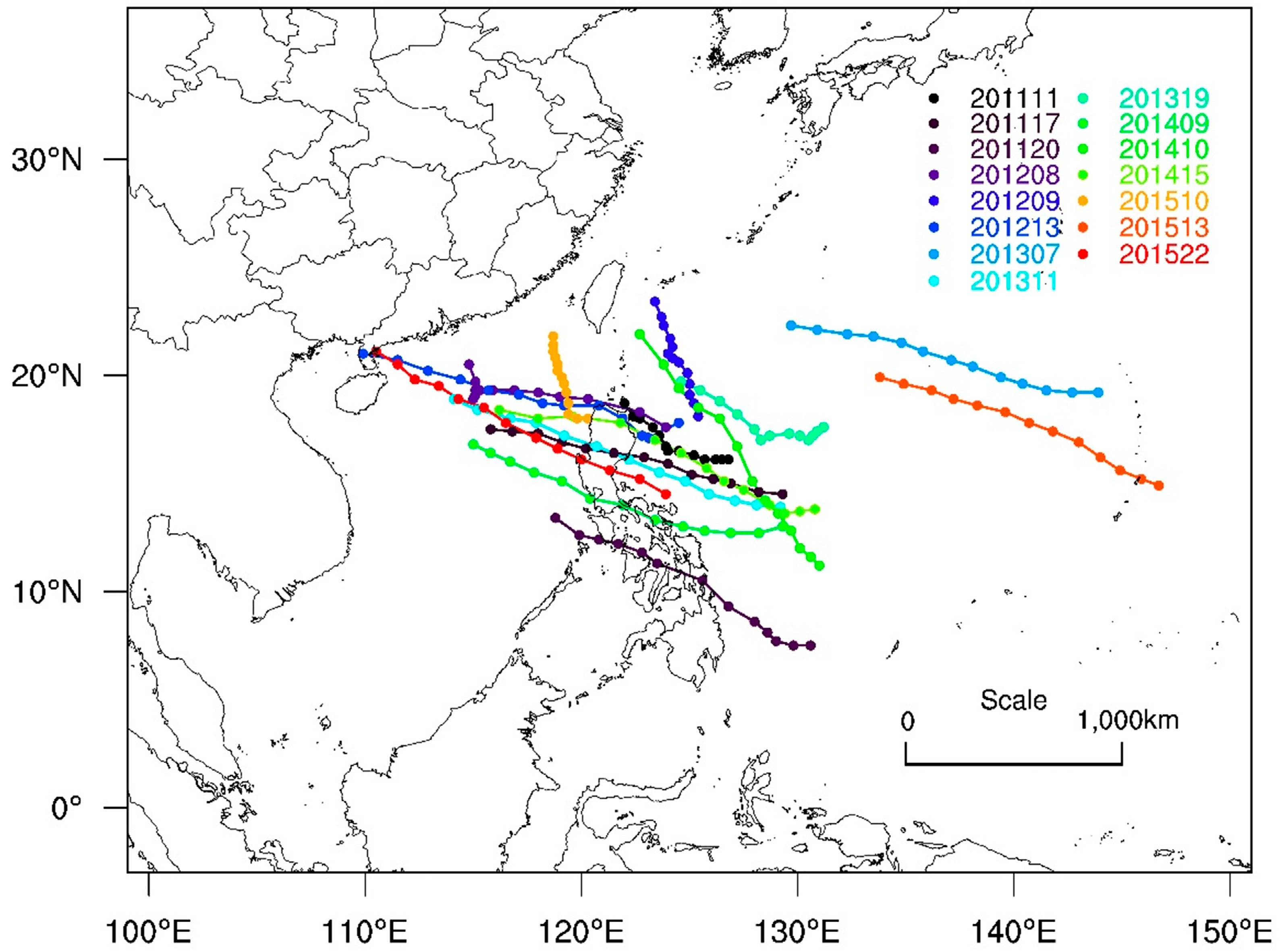
Figure 1. Three-day tracks of the 15 typhoons simulated over the Northwest Pacific Ocean.
Atmosphere 10 00233 g001
Figure 2. The first round of scheme evaluation results for the (ac) track, (df) central sea level pressure (CSLP), and (gi) 10 m maximum wind speed (10 m wind) of 15 typhoons using the Tukey’s test method. For each panel, the evaluation of each scheme is obtained based on the scheme combination simulations, including the scheme, and the pairs of schemes sharing at least one letter are not significantly different between their population means; otherwise, they are significantly different. For the significantly different schemes, the order of their population means at the 5% significance level is A > B > C > D > E.
Atmosphere 10 00233 g002
Figure 3. The fourth round of scheme evaluation results for the (ac) track, (df) CSLP, and (gi) 10 m wind of 15 typhoons using the Tukey’s test method.
Atmosphere 10 00233 g003
Figure 4. Optimization speed and efficiency for the 15 typhoon simulations of track, CSLP, and 10-m wind. Ens1, Ens2, Ens3, and Ens4 represent the four ensembles. Ens5-track, Ens5-CSLP, and Ens5-10m wind represent the optimal ensemble of track, CSLP, and 10-m wind, respectively. (ac) represent optimization speeds of the track, CSLP, and 10 m wind simulations, respectively. (d) represents the improvement rate of Ens5s for typhoon simulation compared to Ens1.
Atmosphere 10 00233 g004
Figure 5. Improvement percentages of the RMSE of Ens5s for the (a) Track, (b) CSLP, and (c) 10-m wind of 15 typhoons, compared to the RMSE of Ens1.
Atmosphere 10 00233 g005
Figure 6. Selected frequency of the different schemes as the best or worst member for the fifth round of scheme combinations for (a) track, (b) CSLP, and (c) 10m wind. The positive bar value represents the frequency of the scheme as the best member, and the absolute values of the negative bar represent the frequency of the scheme as the worst member.
Atmosphere 10 00233 g006
Figure 7. Comparisons of the simulation errors between Ens1 and the optimal scheme combination for the (a) track, (b) CSLP, and (c) 10-m wind of 15 typhoons.
Atmosphere 10 00233 g007
Figure 8. Track of typhoons for (a) Vicente (201208) and (b) Matmo (201410) simulated with the default and optimal scheme combination for the track simulations.
Atmosphere 10 00233 g008
Figure 9. The comparisons of the intensity and track simulations for typhoon Vicente (201208) and typhoon Matmo (201410) using the default and optimal scheme combinations. (af) represent the comparisons of the CSLP, 10-m wind, and track simulations, respectively. The observations are also from the CMA-STI best track dataset for tropical cyclones over the Northwest Pacific Ocean.
Atmosphere 10 00233 g009
Figure 10. Comparisons of the track and intensity simulations for typhoon Megi (201617) and typhoon Nesat (201709) using the default and optimal scheme combinations. (af) represent the comparisons of the track, CSLP, and 10-m wind simulations, respectively. The observations are also from the CMA-STI best track dataset for tropical cyclones over the Northwest Pacific Ocean.
Atmosphere 10 00233 g010
Table 1. Summary of the 15 simulated typhoon cases, including the typhoons’ Chinese number ID, names, and simulation periods *.
NumberTyphoon CasesSimulation Periods
(1)201111 Nanmadol2011-08-24_06:00:00–2011-08-27_06:00:00
(2)201117 Nesat2011-09-25_06:00:00–2011-09-28_06:00:00
(3)201120 Banyan2011-10-10_06:00:00–2011-10-13_06:00:00
(4)201208 Vicente2012-07-20_06:00:00–2012-07-23_06:00:00
(5)201209 Saola2012-07-29_06:00:00–2012-08-01_06:00:00
(6)201213 Kai-tak2012-08-14_06:00:00–2012-08-17_06:00:00
(7)201307 Soulik2013-07-08_06:00:00–2013-07-11_06:00:00
(8)201311 Utor2013-08-10_06:00:00–2013-08-13_06:00:00
(9)201319 Usagi2013-09-17_06:00:00–2013-09-20_06:00:00
(10)201409 Rammasun2014-07-14_06:00:00–2014-07-17_06:00:00
(11)201410 Matmo2014-07-19_06:00:00–2014-07-22_06:00:00
(12)201415 Kalmaegi2014-09-12_06:00:00–2014-09-15_06:00:00
(13)201510 Linfa2015-07-05_06:00:00–2015-07-08_06:00:00
(14)201513 Soudelor2015-08-02_06:00:00–2015-08-05_06:00:00
(15)201522 Mujigae2015-10-01_06:00:00–2015-10-04_06:00:00
* The coordinated universal time was used in this study.
Table 2. Physics parameterization schemes selected for the combinatorial optimization.
NumberMicrophysics (MP)NumberCumulus (CU)NumberPlanetary Boundary Layer (PBL)
OptionSchemeOptionSchemeOptionPBL SchemeSurface (SF) Layer Scheme
12Lin11KF11YSURevised MM5
23WSM322BMJ22MYJETA
34WSM533GF35(1)MYNN2Revised MM5
46WSM645G345(2)MYNN2ETA
58Thompson56Tiedtke55(3)MYNN2MYNN
610Morrison614NSAS66MYNN3MYNN
711CAM5.1799OLD-KF77ACM2Revised MM5
813SBU-YLin 89(1)UWRevised MM5
914WDM5 99(2)UWETA
1016WDM6 1012GBMRevised MM5
Table 3. Selected physics schemes at the fourth round of scheme screening.
NumberMPNumberCUNumberPBL
OptionSchemeOptionSchemeOptionPBL SchemeSF Scheme
12Lin11KF19(2)UWETA
24WSM526Tiedtke212GBMRevised MM5
36WSM6314NSAS
48Thompson
510Morrison
616WDM6
Table 4. Optimal scheme combinations for the simulations of track, CSLP, and 10-m wind.
VariablesMPCUPBL
OptionSchemeOptionSchemeOptionPBL SchemeSF Scheme
Track8Thompson6Tiedtke9(2)UWETA
CSLP4WSM56Tiedtke9(2)UWETA
10-m Wind2Lin6Tiedtke9(2)UWETA
Table 5. Summary of the errors obtained with the six different scheme combinations using each of the six MP schemes, the optimal CU, and the optimal PBL scheme. Bold values represent the optimal variable simulations.
Scheme OptionsRMSE
MPCUPBLSFTrack (km)CSLP (hPa)10-m Wind (m s−1)
2692128.0110.445.96
4692131.289.556.21
6692127.8010.056.29
8692126.1310.296.67
10692130.7910.437.10
16692128.9410.116.09