Article

Characterization of Moisture Sources for Austral Seas and Relationship with Sea Ice Concentration

1
Instituto de Recursos Naturais, Universidade Federal de Itajubá, Itajubá 37500-903, Minas Gerais, Brazil
2
Environmental Physics Laboratory (EPhysLab), CIM-UVigo, Universidade de Vigo, 32004 Ourense, Spain
3
Departamento de Ciências Atmosféricas, Universidade de São Paulo, São Paulo 05508-090, Brazil
4
Instituto de Ciências Ambientais, Químicas e Farmacêuticas, Universidade Federal de São Paulo, Diadema 09913-030, Brazil
5
Instituto Dom Luiz, Universidade de Lisboa, 1749-016 Lisboa, Portugal
*
Author to whom correspondence should be addressed.
Atmosphere 2019, 10(10), 627; https://doi.org/10.3390/atmos10100627
Submission received: 7 August 2019 / Revised: 8 October 2019 / Accepted: 12 October 2019 / Published: 17 October 2019
(This article belongs to the Special Issue Analysis of Oceanic and Terrestrial Atmospheric Moisture Sources)

Abstract

:
In this study, the moisture sources acting over each sea (Weddell, King Haakon VII, East Antarctic, Amundsen-Bellingshausen, and Ross-Amundsen) of the Southern Ocean during 1980–2015 are identified with the FLEXPART Lagrangian model and by using two approaches: backward and forward analyses. Backward analysis provides the moisture sources (positive values of Evaporation minus Precipitation, E − P > 0), while forward analysis identifies the moisture sinks (E − P < 0). The most important moisture sources for the austral seas come from midlatitude storm tracks, reaching a maximum between austral winter and spring. The maximum in moisture sinks, in general, occurs in austral end-summer/autumn. There is a negative correlation (higher with 2-months lagged) between moisture sink and sea ice concentration (SIC), indicating that an increase in the moisture sink can be associated with the decrease in the SIC. This correlation is investigated by focusing on extremes (high and low) of the moisture sink over the Weddell Sea. Periods of high (low) moisture sinks show changes in the atmospheric circulation with a consequent positive (negative) temperature anomaly contributing to decreasing (increasing) the SIC over the Weddell Sea. This study also suggests possible relationships between the positive (negative) phase of the Southern Annular Mode with the increase (decrease) in the moisture that travels from the midlatitude sources to the Weddell Sea.

1. Introduction

Sea ice is any form of ice found at sea that has originated from the freezing of seawater [1] and it is one of the climate system components [2]. At the same time that the sea ice is a result of the interaction of the ocean-atmosphere exchanges, it also causes great influence on the Earth’s climate [3,4,5]. One example is the sea ice impact on the oceanic surface albedo [6], if the oceanic surface is covered by water the albedo is about 10–15% [7], while the albedo can range from 44% to 90% [8] when covered by sea ice. Studies on sea ice, in general, evaluate the extension and/or concentration of the ice.
Around the Antarctic, the sea ice extends to ~19 million km2 in September and retracts to ~4 million km2 in February [9]. Therefore, from the austral winter to the beginning of spring, the area covered by sea ice exceeds the area of continental ice [10]. Different from the Arctic, where a considerable decrease in sea ice extension has been observed in the last three decades, the global Southern Ocean showed a moderate increase until 2014 followed by a decline [11,12]. The long-term trend is not spatially homogeneous since it is positive over the western Ross Sea and negative on the Bellingshausen and Amundsen seas [13]. Some authors have also indicated a dominant positive trend of the sea ice concentration in the austral seas [13,14,15,16].
Sea ice extension and concentration are not only dependent on seasonality. They respond to many different interactive processes in the atmosphere and ocean [13,17], large-scale atmospheric circulation modes [18], as well as the processes associated with climate change [19]. Hobbs et al. [13] present an overview of some of the processes that change the ice extension and concentration such as the advection of heat, the horizontal movement of sea ice by wind and ocean currents, and mixed layer freshwater fluxes such as precipitation. Holland and Kwok [14] found a strong link between trends in ice concentration and ice motion (or winds) and highlighted that more southerly winds could increase the ice concentration through either increased transport of ice from the south or through an atmospheric cooling from the increased advection of cold polar air masses, while more northerly winds would decrease ice transport and cause atmospheric warming.
For the Weddell Sea (which will be a focus of this study), [20,21] have shown that vigorous convective mixing, whereby the upward flux of relatively warm deep waters supplied heat, prevents sea ice formation. Gordon [21] also highlighted that during the negative phase of the Southern Annular Mode (SAM) there is a northward expansion of cold, dry polar air masses from Antarctica, which reduces precipitation and increases surface water salinity. It causes a breakdown of the pycnocline, enabling deep-reaching convection cells that transfer heat from the deep ocean into the surface layer, resulting in a winter ice-free area. On the other hand, in the case of great moisture supply (precipitation), stronger ocean stratification is expected (decrease in the mixing), with a consequent decrease in the ocean heat transport to the surface and a sea ice increase [22]. This line of reasoning also expects that more precipitation means more snow on sea ice, which further increases the ice cover due to snow-ice formation.
Recent studies [23,24] have shown that northerly winds toward the Antarctic region, although transporting moist air, can contribute to the decrease in the sea ice extension and concentration through energy fluxes (vertical and meridional) as well as the movement of sea ice (e.g., [23]). In the latter case, the atmospheric circulation forces the reorganization of the sea ice drift, thus leading to more sea ice convergence (lower sea ice extent) or divergence (higher sea ice extent). Ionita et al. [17] pointed out that the negative anomalies in the sea ice concentration registered in the 2016 austral spring were associated with the enhanced poleward advection of warm and moist air, which leads to strong sea ice melting. Turner et al. [24] associated the sea ice extent and concentration anomalies of this springtime episode with a series of atmospheric circulation anomalies, from September to November 2016, such as a deeper Amundsen Sea Low (ASL) in September, which contributed to greater sea ice retreat than usual in the Weddell Sea, and the amplified planetary waves in October, which were important for the stronger meridional flow, leading to increase the heat flux poleward. A similar idea was proposed by [25], who indicated that the 10-meter wind associated with weather systems is the “chief” thermodynamic and dynamic driver of sea ice variability. However, they do not provide any information related to the meridional moisture flux associated with the weather systems. Meehl et al. [12] also studied the sudden Antarctic sea ice retreat in late 2016 using an atmosphere-only model with a specified convective heating source (to represent intensified convective activity) in the eastern Indian/western Pacific Ocean. According to Meehl et al. [12], the sea ice retreat in 2016 can be associated with 3 factors: (1) anomalous atmospheric Rossby wave with a consequent teleconnection pattern around the Antarctic, and warm-moist southward surface winds promoting sea ice convergence, (2) warmer surface water transported southward, and (3) low frequency (decadal) signal of negative wind stress trends superimposed by the positive trend of the SAM and the negative phase of Interdecadal Pacific Oscillation forced upward movement of subsurface warmer water.
Although the teleconnection patterns appear to be important for the Southern Oceans ice retreat in spring 2016, there are climatological studies indicating that the large scale modes do not explain a large part of the sea ice variability over the whole Southern Ocean [26]. Only certain sectors of this ocean respond to different atmospheric modes [18]. Raphael and Hobbs [18] emphasize that the atmosphere-cryosphere relationship has both an immediate and a time-lagged response. The immediate response is due to the horizontal advection and vertical fluxes of energy that affect sea ice, while the time-lagged response is related to the influence of the atmosphere on the ocean, and this, through heating/cooling, would later affect the increase/decrease in the ice. For example, [27] observed that the enhancement of the zonal winds in South Pacific high latitudes during springtime allows an earlier melt of the ice in the western Ross Sea, with a consequent increase in the absorption of solar radiation by the ocean and reduced ice cover the next autumn.
Many investigations of the sea ice around the Antarctic analyze the austral seas individually [6,18]. For example, sea ice in the Weddell Sea (eastern Antarctic Peninsula) is perennial, which is a result of the convergence of sea ice due to the Ekman transport associated with the Weddell Gyre [28]. Some authors [14,29,30] associated the ASL impacts on the sea ice in the Weddell Sea through the near-surface winds: north winds generally contribute to positive temperature anomalies and decreases in the sea ice concentration.
Among the multiple atmospheric and oceanic drivers controlling the sea ice variability, little attention has been paid to the moisture transport from the extratropics to the Southern Ocean [23,31,32], a mechanism proposed to have an important role in the Arctic atmospheric hydrological system e.g., [33,34], with implications for the Arctic Sea ice extension. Indeed, atmospheric moisture transport is a primary source of water in polar regions, and, according to [23], through the cloud radiative forcing, it directly or indirectly affects the snow, sea ice, and ice sheet. For the first time, a study presents the climatology (for the period 1980–2015) of the main moisture sources for the Southern Ocean seas using a Lagrangian approach [35,36]. Moreover, it focuses on the relationships of the transported moisture with sea ice concentration.

2. Methodology

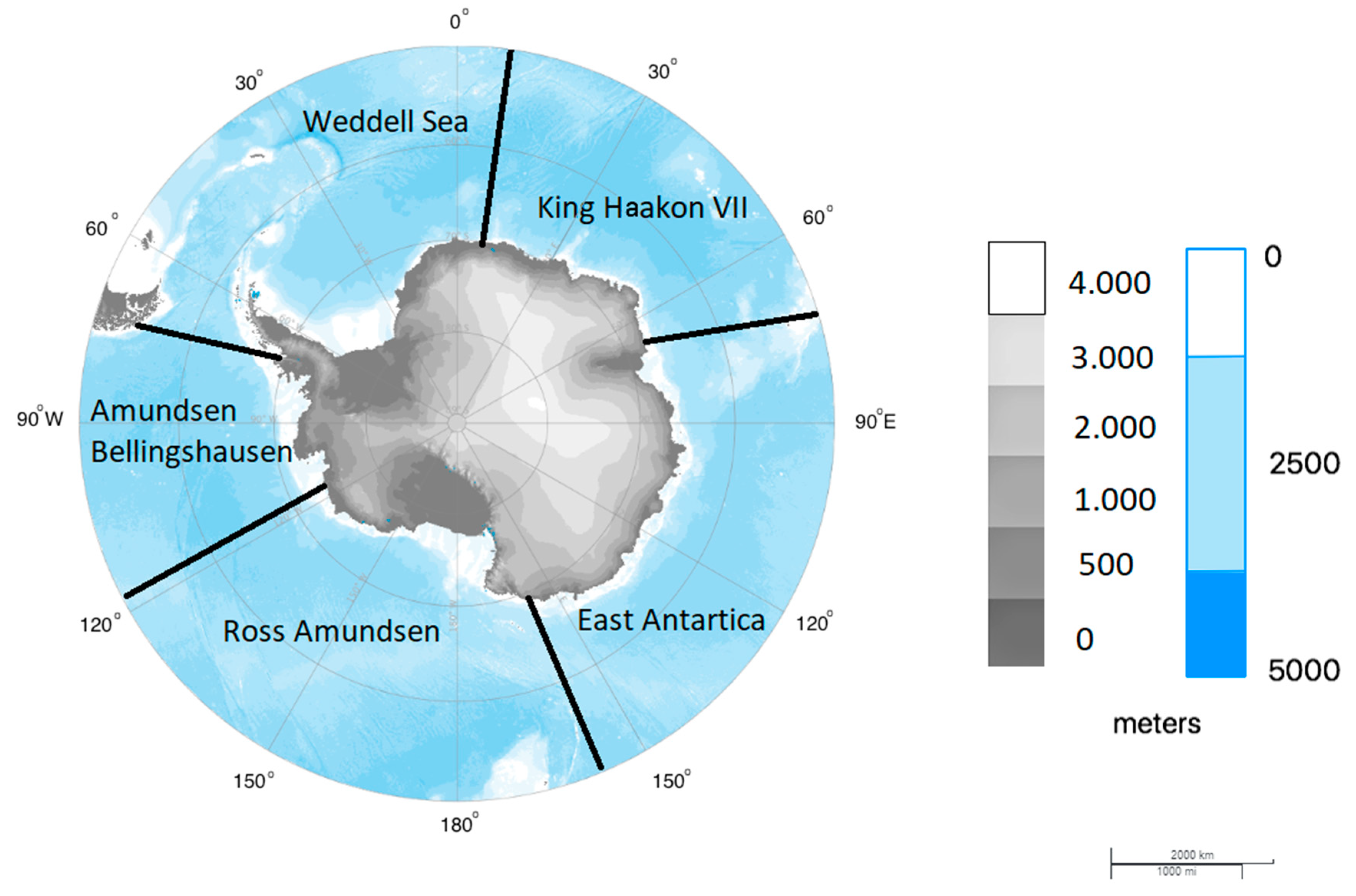
2.1. Data and Area of Study

As previously established, one aim of this study is to find the relationship between moisture transport and sea ice concentration (SIC) over each of the austral seas. According to the National Snow & Ice Data Center [37], SIC is a unitless term describing the relative amount of area covered by ice, compared to a specific reference area, and it is typically reported as a percentage (0 to 100), a fraction (0 to 1), or sometimes in tenths (0/10 to 10/10). In these scales, 0 means that there is no ice, while a reference area completely ice-covered is represented by 1 (or 10/10 or 100). The period of study is 1980 to 2015, and the SIC is obtained from satellite using the Special Sensor Microwave/Imager (SSM/I) and Special Sensor Microwave Imager and Sounder (SSMIS) sensors on the U.S. Department of Defense Meteorological Satellite Program (DMSP) platforms. These data are processed by the National Snow and ICE Data Center from NOAA/NSIDC Climate Data Record (CDR) [38], having monthly frequency on a 0.25° regular horizontal resolution.
ERA-Interim reanalysis from European Centre for Medium-Range Weather Forecasts (ECMWF, [39]), which is considered the state-of-the-art reanalysis in terms of the hydrological cycle [40,41], is used for the moisture sources identification and other analyses.
The moisture sources identification for austral seas focuses on specific areas (which are defined in Section 2.3) of each sea around the Antarctic (Figure 1). The domains defining each sea follows [18] and they are only used as geographic referential. Raphael and Hobbs [18] used the standard deviation of sea ice extension to specify the boundaries of the austral seas as: King Haakon VII (16° E–69° E), East Antarctic (70° E–162° E), Ross/Amundsen (163° E–110° W), Amundsen/Bellingshausen (109° W–68° W), and Weddell (67° W–15° E). Here, for brevity, we will call the seas Ross/Amundsen “Ross”, Amundsen/Bellingshausen “Amundsen”, and King Haakon VII “King”.

2.2. Lagrangian Approach for Moisture Transport Identification

The moisture transport calculation is based on the method developed by Sthol et al. [35,42], which uses the Lagrangian FLEXible PARTicle dispersion model (FLEXPART, [36]). FLEXPLART was originally developed to study the transport of particles, but during recent decades, it has been successfully used to analyze moisture transport [43]. The input data to the FLEXPART is the ERA-Interim reanalysis [39] with 61 vertical levels (top of the atmosphere located at 0.1 hPa) and interpolated to the 1° of horizontal resolution every 6 hours (at 00, 06, 12 and 18 UTC). Due to the importance of temporal resolution for the accuracy of the calculation performed by FLEXPART [36], intermediate 3h-forecast data from ECMWF are also used.
In FLEXPART, finite elements of volume with equal mass (hereafter “particles”) are homogeneously distributed across the atmosphere. It means that the number of “particles” is proportional to the air density, and hence more “particles” are initially near the surface. The forward (or backward) trajectories are then calculated using a 3D wind field (zonal, meridional and vertical components). The particles selected over each area of study form part of a global experiment in which a total of around 2 million particles were globally distributed and moved for the period 1980–2015. This global experiment was previously used in many analyses over different areas eg., [44,45,46,47,48] including Antarctica [32,49].
Once the particles and their trajectories are selected over an area of interest, the methodology developed by [35,36] is applied. In the backward mode, the trajectories of the particles indicate the sources of moisture for a given area. The forward option computes the moisture transported from the sources into each target region (which helps to compute the moisture that forms precipitation and are called sink regions–see Section 2.4). In this study, we use both options.
For each particle along its trajectory, the latitude, longitude, altitude, and specific humidity (q) are recorded according to the temporal resolution of the input data. The changes in moisture for each particle through the difference between the evaporation (e) and precipitation (p) are calculated for every time step. These changes in time along the individual trajectories are given by:
( e p ) k = m d q d t
where ( e p ) k indicates the rate of increase (e > p) or decrease (e < p) in moisture along the trajectory of each particle k and m is the mass of each particle. Adding the ep in an atmospheric column over a given area (A) for all the tracked particles residing in it, the surface freshwater flux (E − P) associated with those particles is:
E P = k = 1 K ( e p ) k A
where the water budget is calculated for all K particles that reside above the area A. According to [43], this methodology allows us to identify the evaporative source and sink regions for a given area (see [43] for a review on the advantages/disadvantages of different techniques to estimate moisture sources). Although the Lagrangian techniques are based on the estimation of the E − P budget, they have been also used extensively in dozens of papers with great success for the precipitation estimation through the humidity coming from the source to the target regions for global [50,51] or regional studies [45,52,53].

2.3. Backward Trajectories: Identification of the Moisture Sources for the Southern Ocean Seas

As an initial step, moisture sources for the five individual Southern Ocean seas are identified using the backward trajectories. Only the areas covered by the SIC equal or greater than 0.1 (10%) are used as the target area inside every austral sea. These target areas vary monthly due to the SIC annual cycle (and other variabilities that cause changes in the SIC). With this in mind, all particles residing over each sea (the target regions) are tracked backward in time over 10 days to assess where the particles gain moisture. The period of tracking is limited to 10 days since it is the average residence time of water vapor in the atmosphere [54]. The total atmospheric moisture budget (E − P) integrated over the 10 days of tracking (i10) and averaged over the period of interest (annual or seasonal), hereafter named (E − P)i10, shows where the particles acquired or lost moisture before reaching the target areas. Where (E − P)i10 > 0, the air parcels over that area gain moisture from the surrounding environment (through evaporation from the surface to the atmosphere and also in the atmosphere due to changes in the water phase such as rain evaporating as it falls into a dry layer). Therefore, the moisture sources are characterized by (E − P)i10 > 0. Annual and seasonal sources are selected, considering austral seasons: summer as December–January–February (DJF), autumn as March–April–May (MAM), winter as June–July–August (JJA), and spring as September-October-November (SON).

2.4. Forward Trajectories: Main Moisture Sinks in the Southern Ocean Seas

In order to investigate the total moisture contribution over every austral sea, the moisture sources are defined taking into account the 75th percentile of the (E − P)i10 > 0 annual mean value (and it is considered a threshold). The areas with moisture ((E − P)i10 > 0) greater than this value (black contours in Figure 2) are used as the initial regions for the forward tracking. From these areas, the particles are tracked forward for 10 days and where (E − P)i10 < 0, they lose moisture (i.e., through precipitation and changes in the water phase) characterizing the moisture sink.
Although the area of the SIC greater than a threshold varies monthly, the moisture contribution may affect the sea ice in different ways, leading to its formation or melting. For this reason, it is interesting not only to analyze the contribution over the total sea ice covered areas (SIC value equal to 1). In addition, since we are also interested in understanding the SIC, target areas in the forward analysis are represented by the annual maximum region with SIC values equal or greater than 0.1, which occur in September (blue areas in Figure 2). Therefore, for each sea, the SIC seasonality is investigated in the same target area over the year. In the results section, the values of the moisture sink are multiplied by −1 to facilitate interpretation.

2.5. Moisture Sink and Sea Ice Concentration

The relationships between the moisture sink and the SIC are explored through the climatological annual cycle, trends, and the Pearson correlation coefficient (with and without month-lag). Details about the lag-correlation method are in Section 3.2. Additional analysis is carried out for the Weddell Sea, where previous studies have proposed different mechanisms for SIC variability [20,21,22]. For this sea, the periods with low and high SIC are identified (and considered to be extreme events), using percentiles of 20% (P20) and 80% (P80), respectively, and the relationship with the moisture sink is discussed. These percentiles are obtained from the monthly moisture sink (i.e., (E − P)i10 < 0) anomalies, i.e., monthly values minus the mean annual cycle. Moreover, the month with the highest frequency of P80 (P20) moisture sink events is selected to evaluate the atmospheric and SIC patterns through composites. Possible connections of the moisture sink and SAM are also investigated using the monthly teleconnection index provided by the Climate Prediction Center (NOAA) and available on https://www.cpc.ncep.noaa.gov/products/precip/CWlink/daily_ao_index/aao/monthly.aao.index.b79.current.ascii.

3. Results

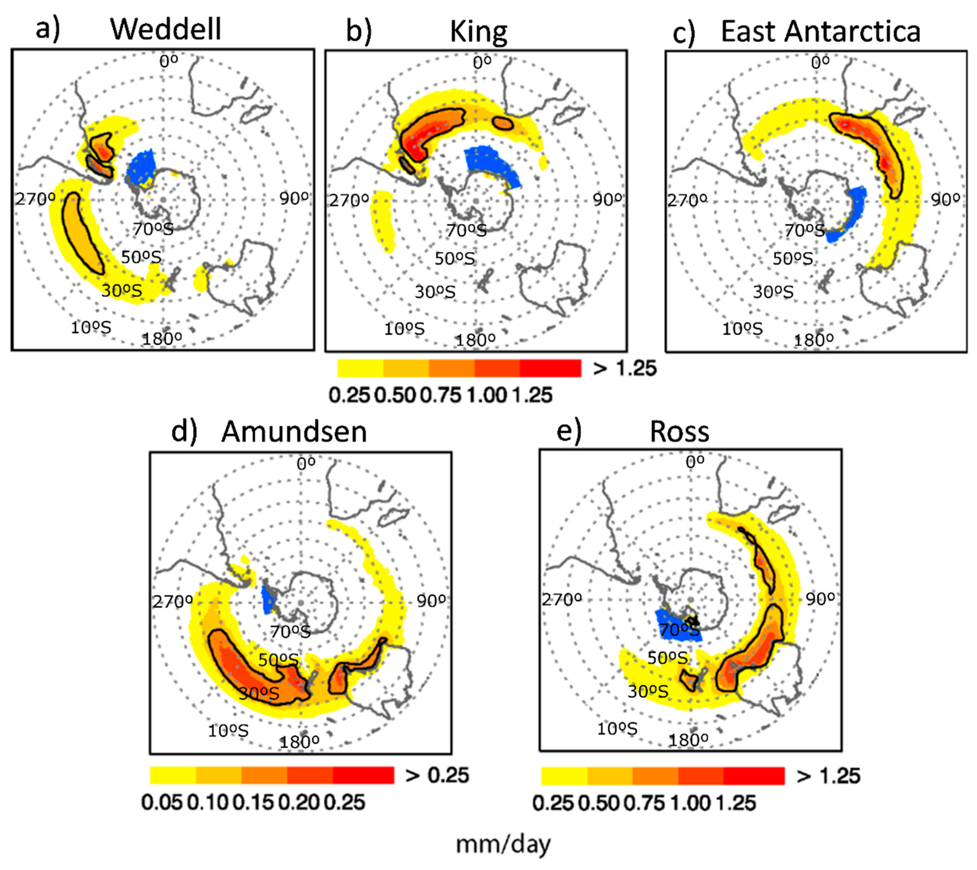
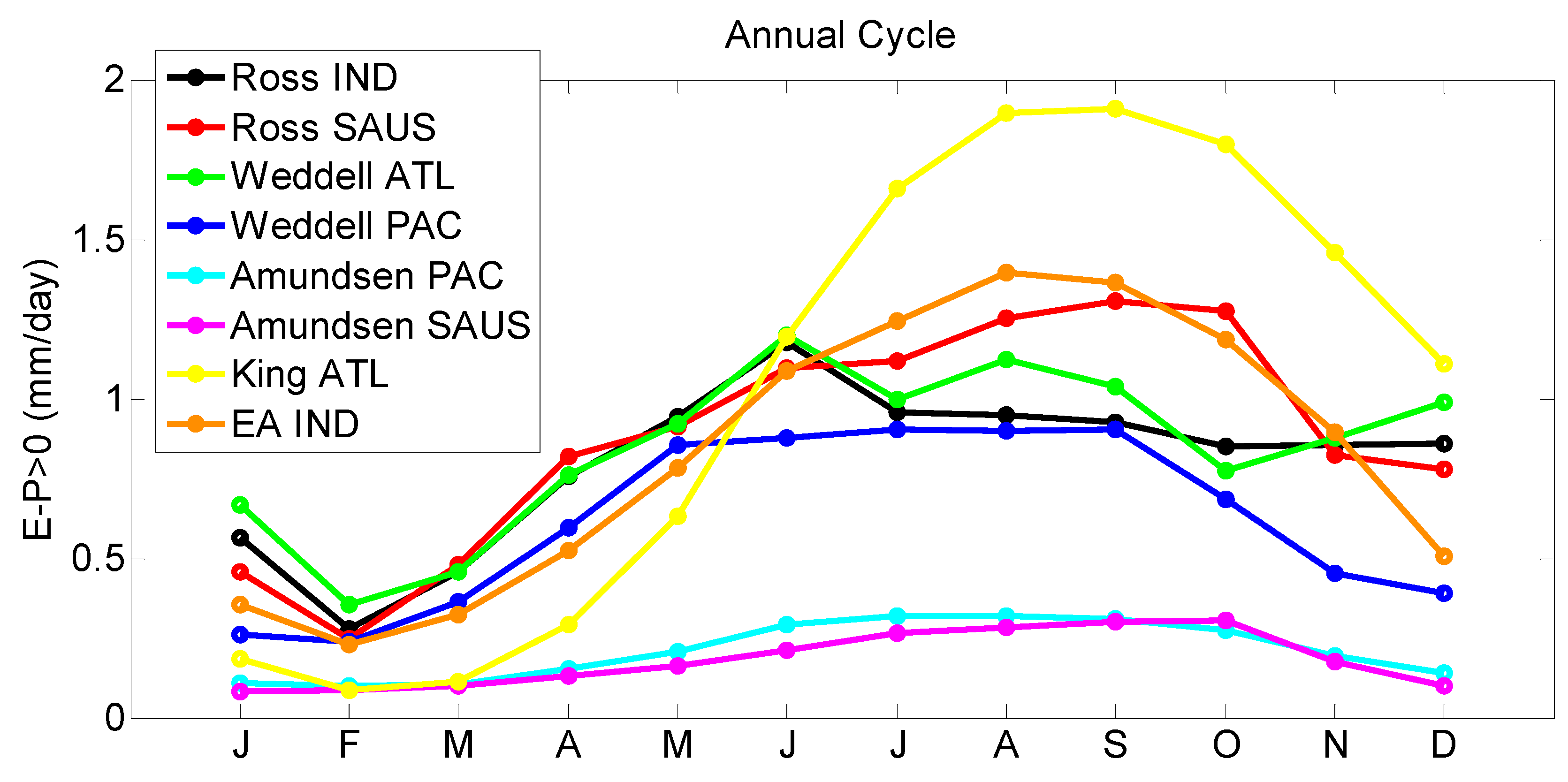
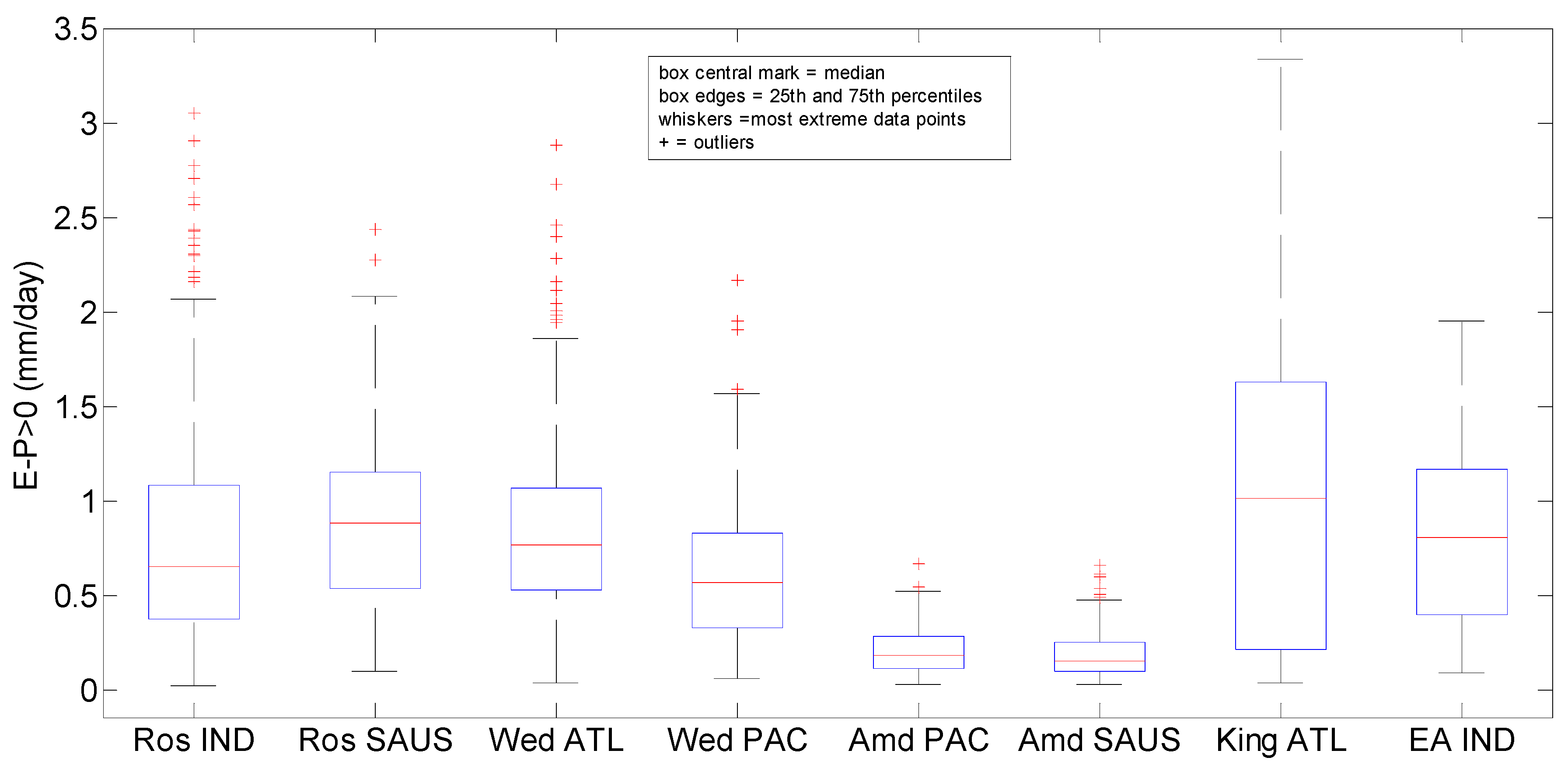
3.1. Main Features of the Moisture Sources

Backward Analysis: Identification of Moisture Sources for the Southern Ocean Seas

Figure 2 shows the annual climatology of the moisture sources for each austral sea, i.e., the regions presenting the atmospheric water budget values greater than zero ((E − P)i10 > 0) considering 10 days backward integration. The main moisture sources are located over the extratropical latitudes, in general, north-westward of the target areas. Therefore, the moisture sources are linked to the preferential path of the storm tracks, which is from west to east during all months of the year [31,55,56]. These sources are coherent with a number of case studies. For example, [31] showed that the strong cyclones are responsible for moisture transport toward Antarctica exceeding the mean values, with higher transport to East Antarctica and the Amundsen-Bellingshausen seas.
According to Figure 2, the Weddell, Ross, and Amundsen seas have two moisture sources, while King and East Antarctica have only one. The Weddell Sea receives moisture from the Pacific (PAC) and Atlantic (ATL) Oceans, the Amundsen’s moisture sources are from PAC and southern Australia (SAUS), the Ross receives moisture from the Indian Ocean (IND) and SAUS, the King’s moisture sources are from ATL, and the East Antarctica’s from IND (Figure 2). It is interesting to note that for the Weddell and King Seas (Figure 2a,b) there is a weak moisture source poleward of the target area (and for this reason they are not included in the following analysis), which is likely related to katabatic winds. Most of the moisture sources are more intense during austral winter-spring and weaken during autumn-summer (figures not shown). The seasonality is weaker and less evident for moisture coming from the Pacific to the Amundsen Sea.
The annual cycle of the moisture sources (i.e., the moisture contribution from the source into the overlying atmosphere) is obtained as the average over the area delimited by the annual 75th percentile (black lines in Figure 2) of the monthly values of (E − P)i10 > 0. In Figure 3, the annual cycle of the moisture sources of the Ross SAUS, the King ATL, and the East Antarctica IND are characterized by strong seasonality, presenting higher values between July–October and lower ones from January-March. Comparatively, from July–October greater intensity of the moisture sources is noted in the King ATL due to both more intense values and larger areas of the sources as shown in Figure 2. The other moisture sources (the Weddell PAC-ATL and Ross IND), although with peaks during May–October, present weak seasonality, while the two moisture sources from Amundsen are the weakest and are almost constant over the year (Figure 3).
The boxplot of the mean monthly moisture sources from 1980 to 2015 is shown in Figure 4. King ATL, East Antarctica IND, and Ross IND present a higher spread of the monthly values (larger differences between 25th and 75th percentiles), while Amundsen SAUS and PAC the lower spread. Figure 4 further shows the great presence of extreme events in the moisture sources in most of the areas, with slightly higher frequency in King ATL. The Weddell ATL and Ross IND have a higher occurrence of outliers compared with the other sources.

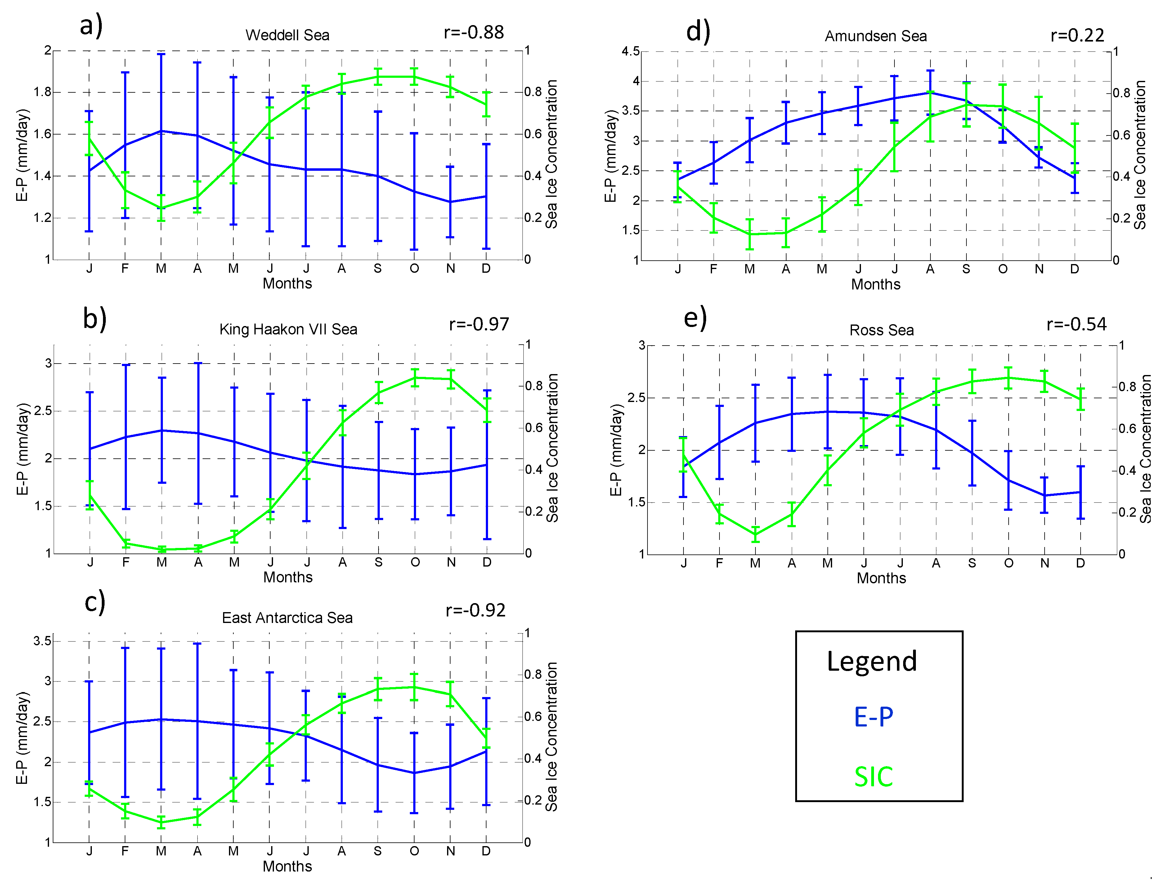
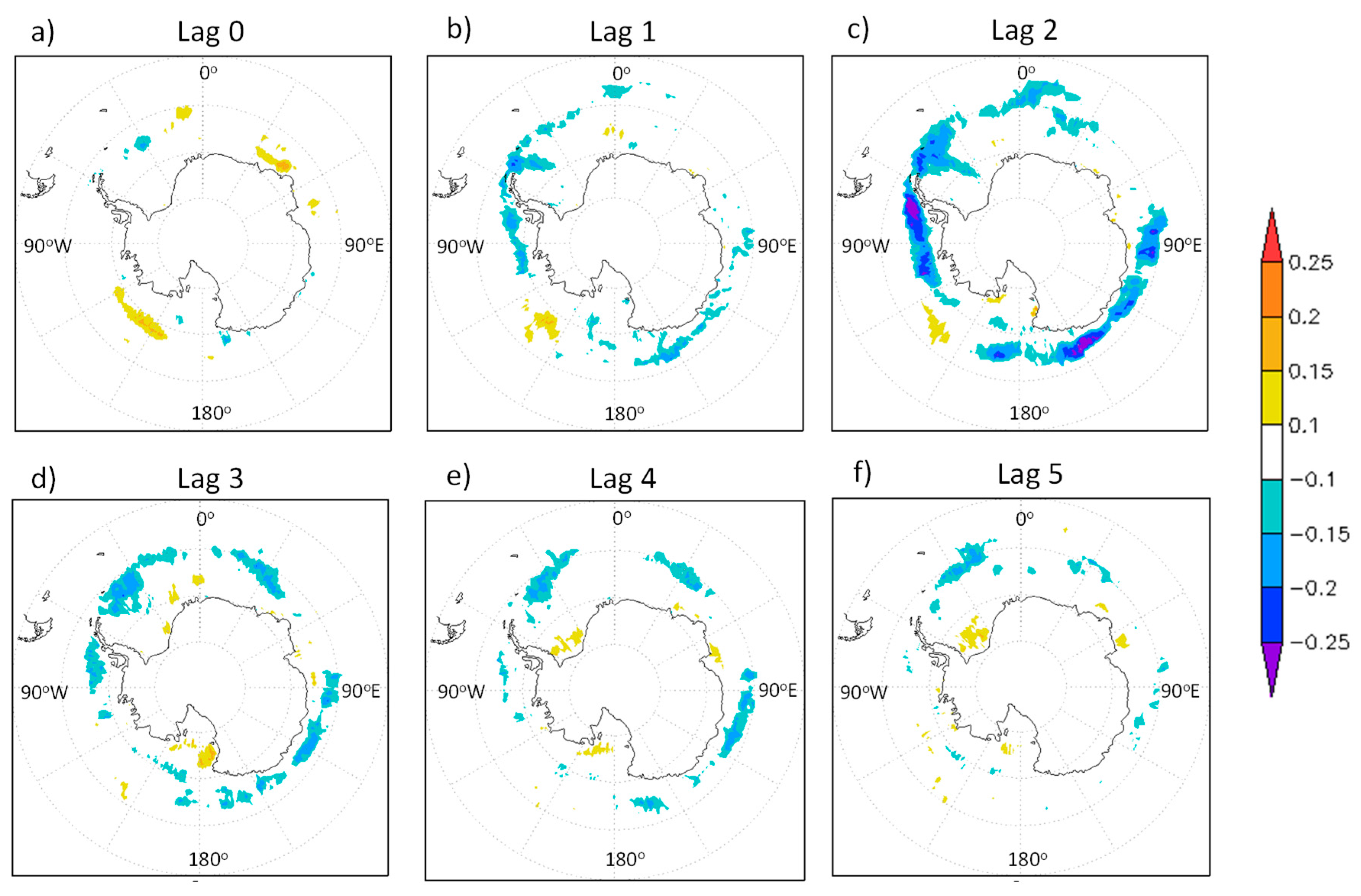
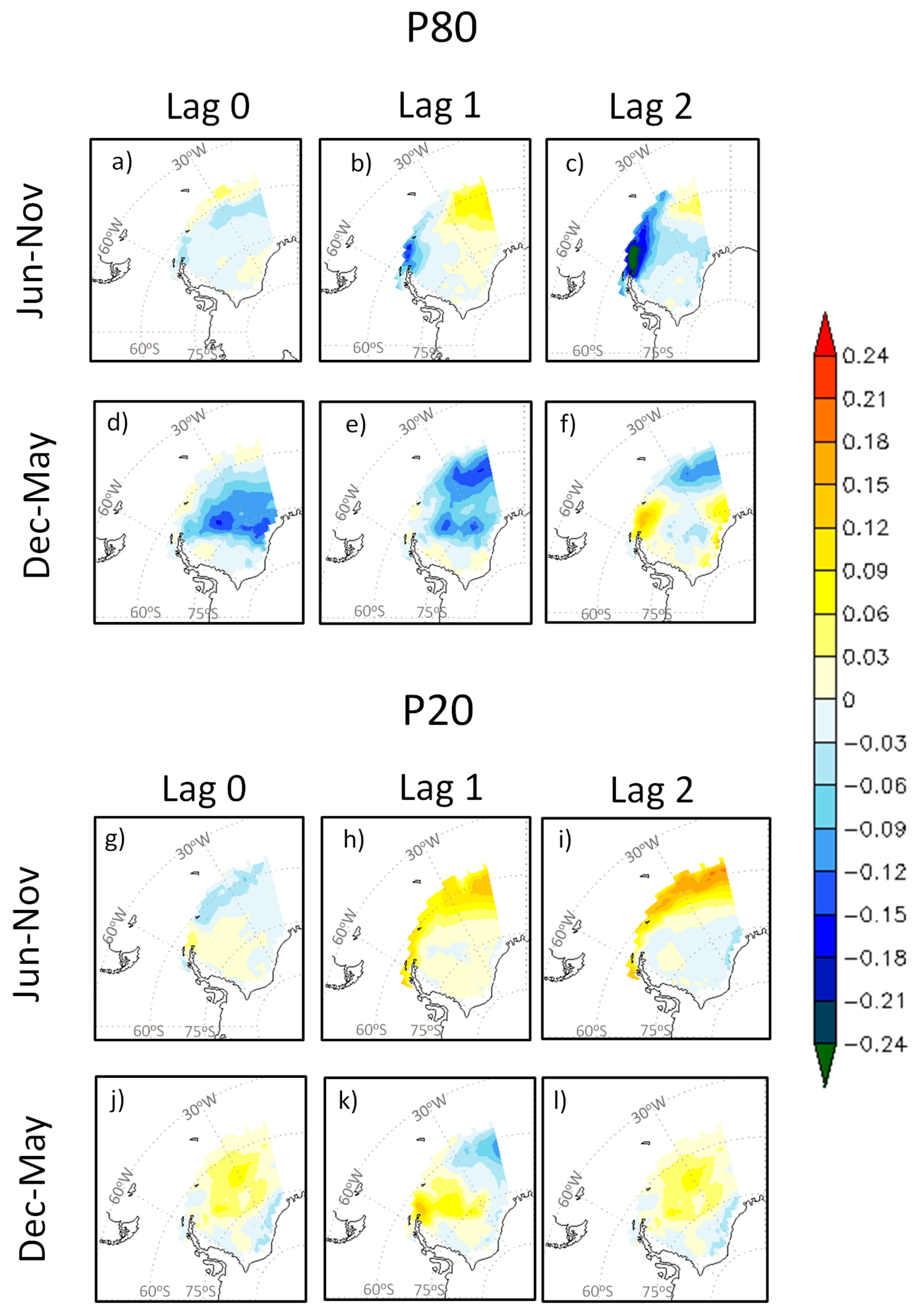
3.2. Forward Analysis: Relationships Between the Moisture Sink and the SIC

In the analysis of moisture sinks, for all seas with two moisture sources, the time series are added (for example, for the Ross Sea we added the IND and SAUS moisture sinks to obtain only one time series). Figure 5 shows the annual cycle of the moisture sink (moisture arriving in the target areas from source), obtained from forward trajectories ((E − P)i10 < 0), over the maximum annual area with sea ice concentration equal or greater than 0.1, which occurs in September (blue area in Figure 2). To facilitate the interpretation of the results, the moisture sink values are multiplied by −1. The moisture sink annual cycles have different patterns from those of the moisture sources (Figure 3), where the oceans have maxima from July to October. For the moisture sinks, the annual cycles are relatively flat over much of the year, presenting weak peaks as a function of the sea. The Weddell, King, and East Antarctica seas have a weak maximum from February to April (Figure 5a–c), while in the Ross Sea (Figure 5e) it is displaced to April–June, and in the Amundsen Sea to August (Figure 5d). On the other hand, the minimum amount of the moisture sink occurs from September to December (Figure 5). In terms of the average, the moisture sink is higher and lower, respectively, in the Amundsen and Weddell seas. These annual cycle shapes of the moisture sink, with the maximum at the end-summer/autumn and the minimum in spring-begin/summer, are similar to those in the Arctic [34]. As moisture sinks over the target areas are mainly associated with precipitation, we can compare it with precipitation climatology over the Southern Ocean. In this context, the slight maximum of the moisture sink in the austral autumn in most of the austral seas (Figure 5) agrees with the precipitation climatology southward of 67.5° S [57]. Considering more regional comparisons, the relatively weak seasonality of the moisture sink in East Antarctica (Figure 5c), with a slight peak in the austral autumn months, is in agreement with observations of rainfall in the Macquarie Island located in this sea [58]. The maximum of the moisture sink between winter and spring in the Amundsen Sea (Figure 5d) is also observed in the rainfall at the Rothera station located in the Antarctica Peninsula on the border of the Amundsen Sea [59].
The moisture sink presents strong interannual variability, as measured by the standard deviation of the monthly values, in most of the seas (Figure 5). Moreover, the interannual variability of the moisture sink is higher over all months of the year in the Weddell, King and East Antartic and weaker in the Amundsen and Ross seas.
Comparing the annual cycles of the moisture sink with those of the SIC, in general, there is an inverse pattern: the maximum SIC occurs when the moisture sink is weaker (Figure 5). This behavior is reflected in the negative and high values (from −0.54 to −0.97) of correlation coefficients (top of Figure 5) in most of the seas, except the Amundsen Sea (0.22). In other words, the moisture seems to make a negative contribution to the SIC over the blue area displayed in Figure 2. This result is similar to [34] for the Arctic region and the case study performed by [23,24] for the austral seas. Figure 5 further shows that the SIC in the Weddell Sea has stronger interannual variability (as shown by standard deviation bars) from January-June, and equally large variability is observed in the Amundsen Sea throughout the year. For the Weddell Sea, the higher interannual variability of the SIC is observed in the period of the greater moisture sink, while in the Amundsen Sea it occurs in the periods of both higher and lower moisture sink. The King and East Antarctic seas register greater SIC interannual variability in the months of minimum moisture supply (July–December). A more complicated pattern is noted in the Ross and Amundsen seas where the SIC interannual variability is greater, respectively, from May-October and July–December.
For a better understanding the relationship between the SIC and the moisture sink, the Pearson correlation coefficient is computed considering different time lags (months), i.e., the monthly mean moisture sink time series are fixed in time, and the SIC are displaced from 1 until 6 months ahead (Table 1). The correlations are calculated for the time series of the anomaly, i.e., the mean annual cycle is subtracted from the time series. The p-value (α = 0.05) is also calculated as an indication of the statistical significance of the correlations. According to Table 1, the higher negative and statistically significant correlations occur at a 2-month lag, except for the 4-month lag in the Ross Sea.
For the time series including all months of the year, Figure 6 presents the correlation maps (correlations between the anomalous moisture sinks and the SIC in each sea, which were merged to provide only one map) for the lags from 0 to 5 months. Only the statistically significant values are shown. For this reason, in general, there is no information near the Antarctic coastline. As expected from Table 1, the negative correlations are dominant in almost all austral seas, and they are higher (in absolute value) in the northern sector of the sea ice edges. Considering the time lags, negative correlations increase (in absolute value) from lag-0 to lag-2, decreasing afterwards. At lag-2 the more intense negative correlations expand in the north-south direction covering a larger area compared to the other lags. Figure 6 also reveals a weaker but persistent positive correlation, from lag-0 to lag-2, between the moisture sink and the SIC over the northern limit of the Ross Sea.
The trends of the monthly moisture sink in each austral sea and the SIC are also evaluated. For this reason, the slope of the time series is computed using Sen’s formulation [60], while its 95% statistical confidence level is provided by the nonparametric test from Man Kendall [61,62,63]. The trends are listed in Table 2, where statistically significant values are highlighted in bold. The monthly moisture sink over the Weddell and King seas presents a positive trend, which is statistically significant only in the Weddell Sea. On the other seas, the trend is negative, and they are not statistically significant. On the other hand, there is a positive and statistically significant trend of the SIC in most austral seas, except in the Amundsen Sea, which presents a negative trend in agreement with [13]. The positive trend in the SIC is also documented in several studies [64,65,66].

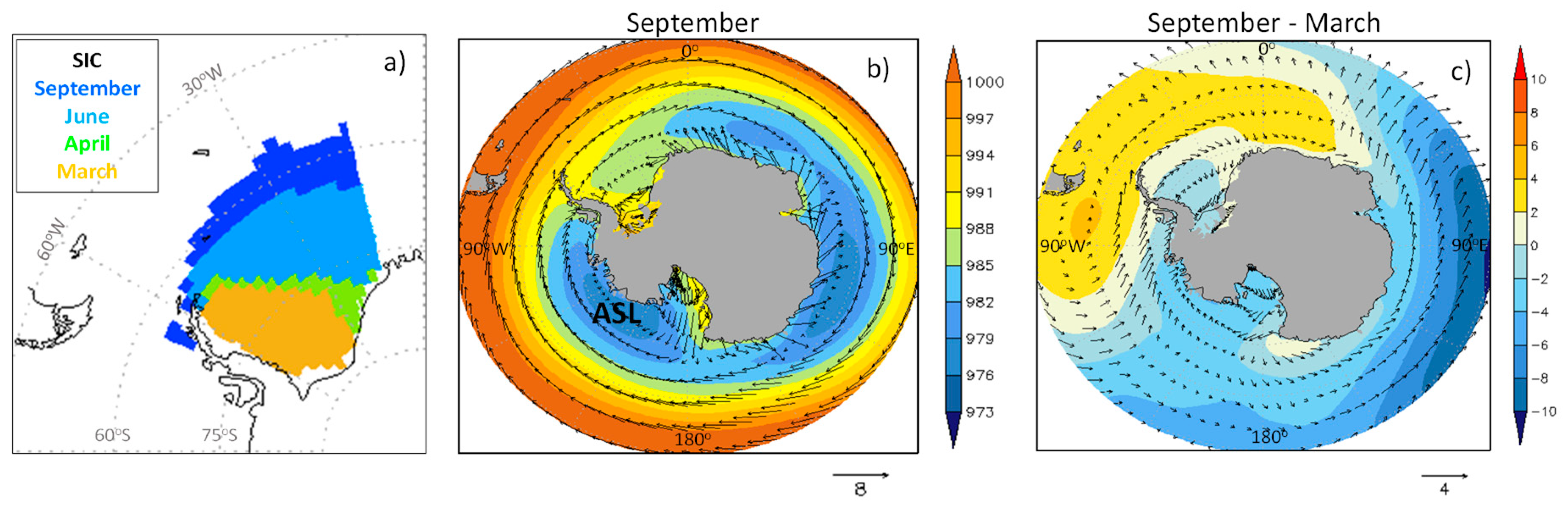
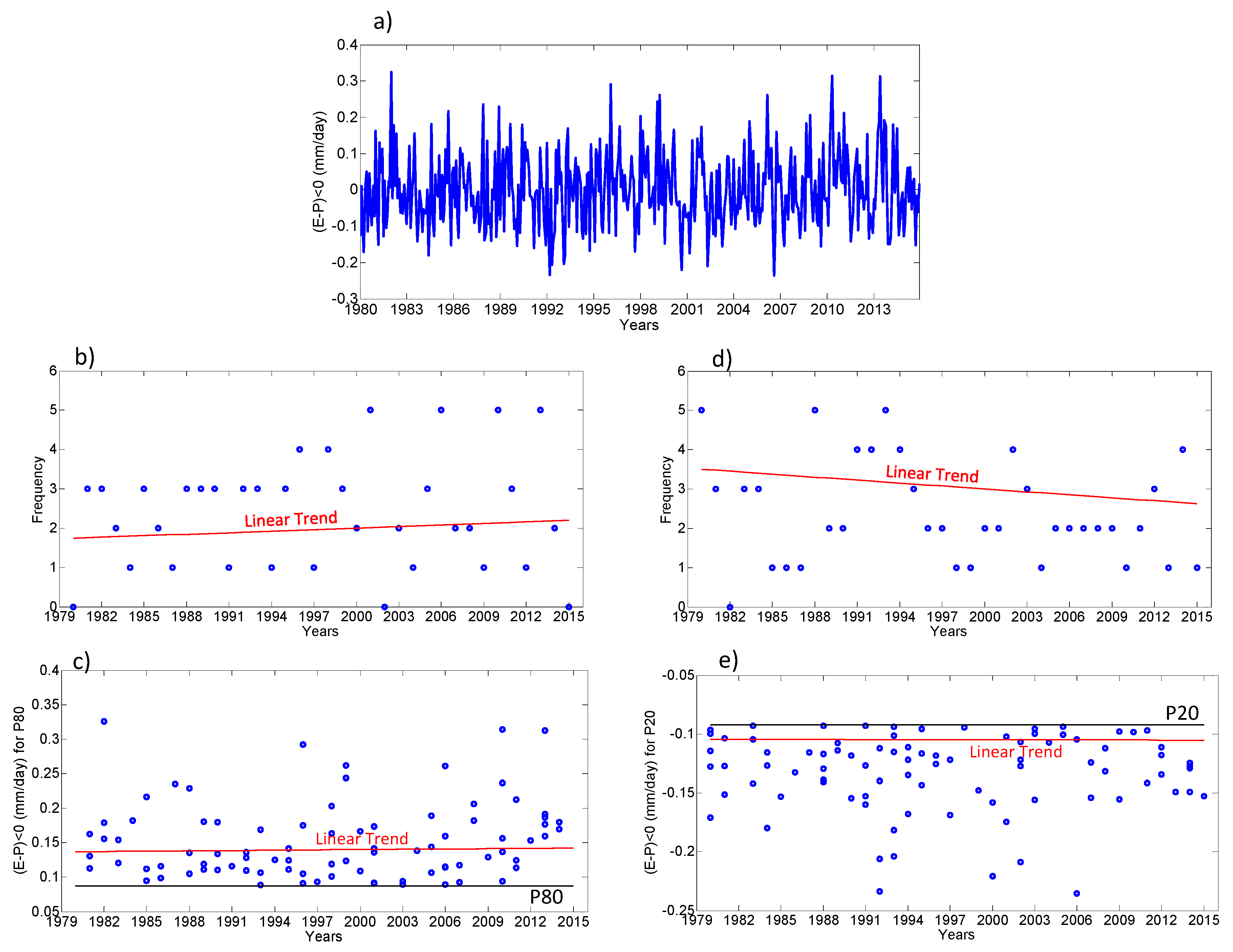
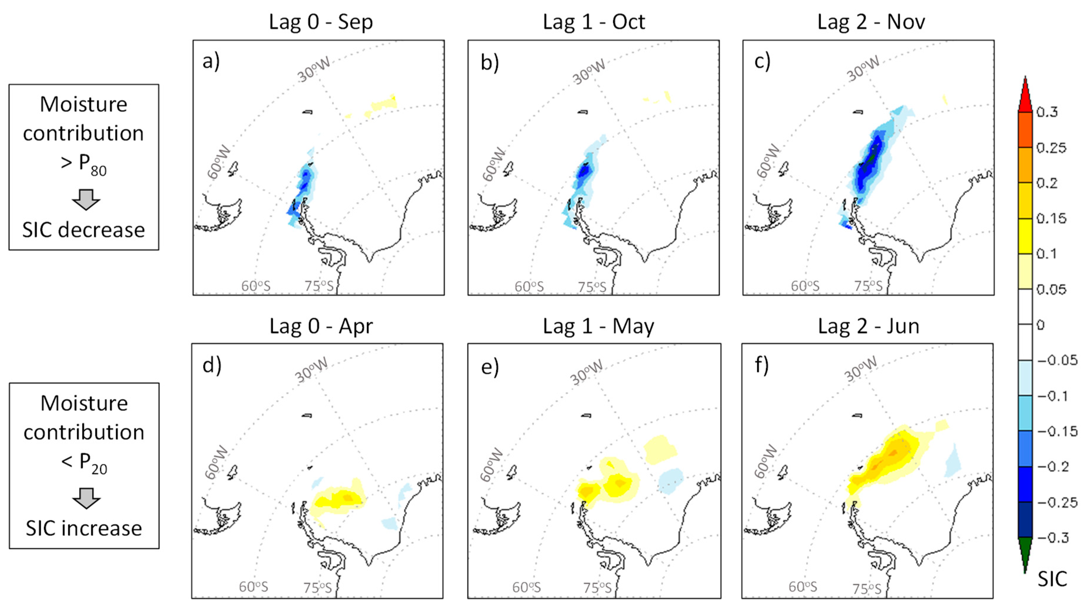
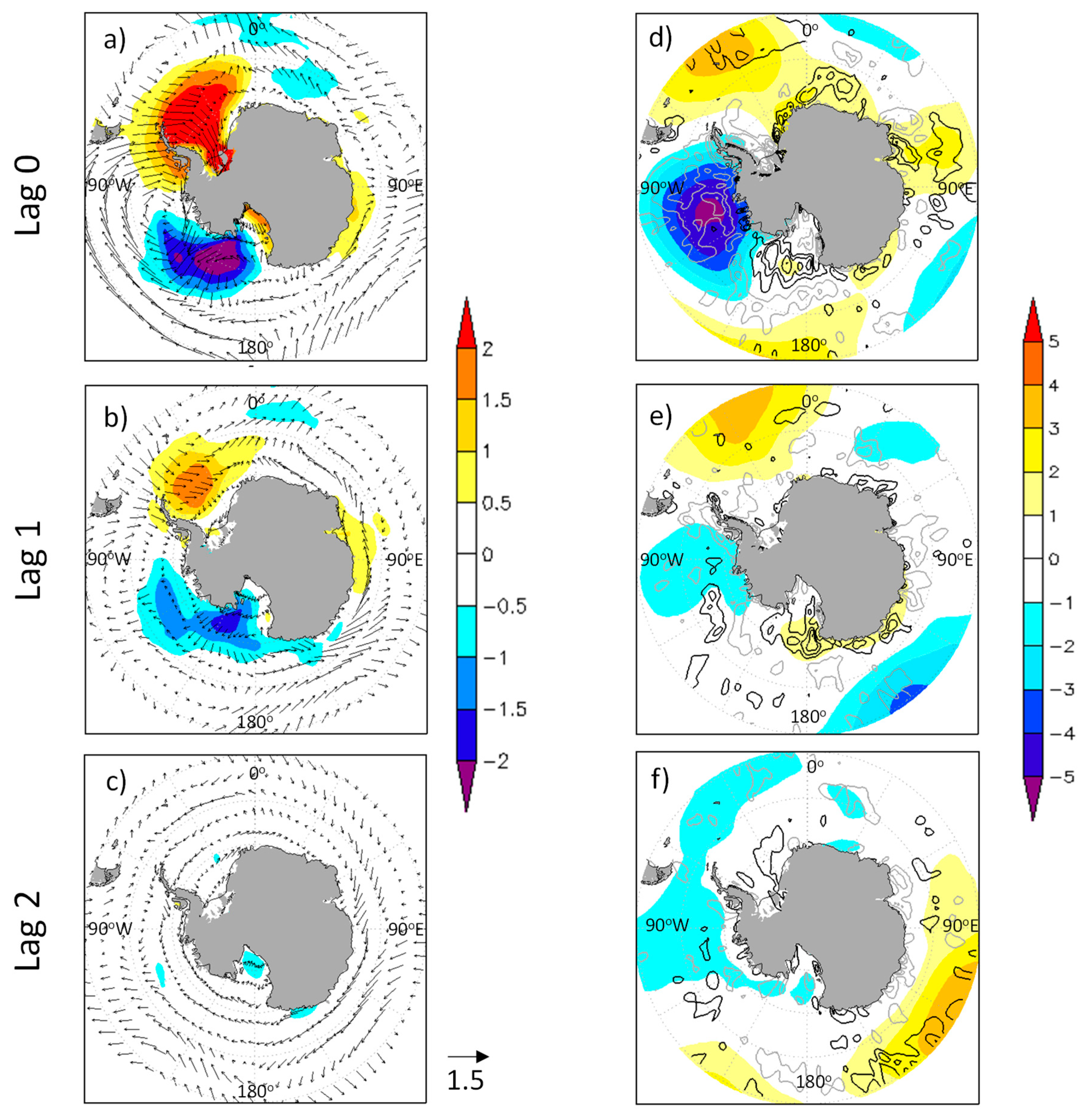
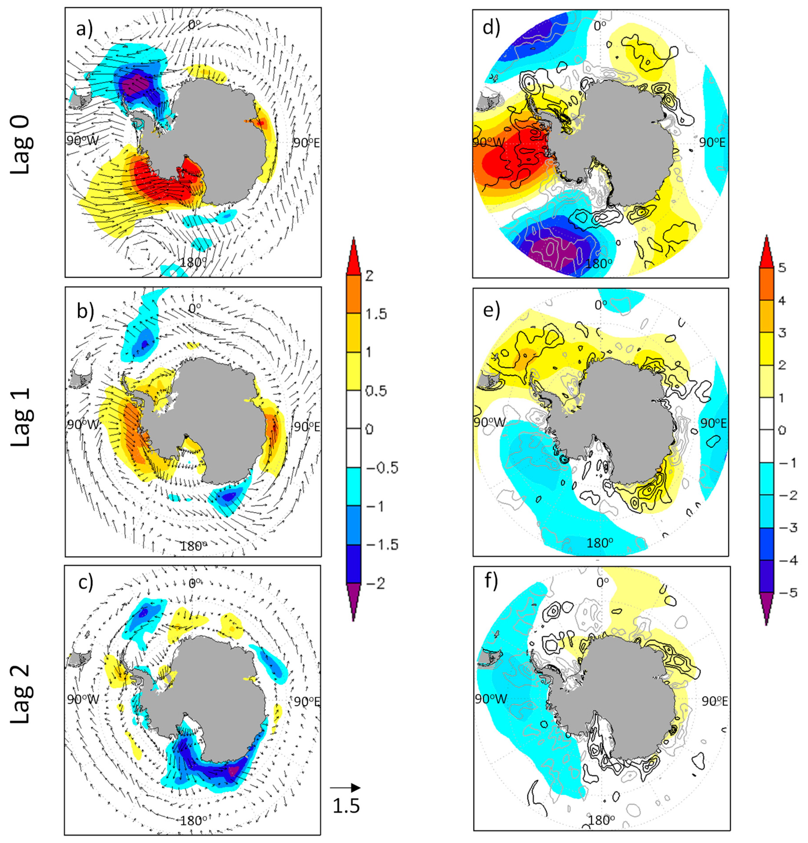
3.3. Extremes in the Moisture Sink for the Weddell Sea and the SIC

For the Weddell Sea, Figure 7a presents the area occupied for SIC values exceeding 0.4 for four different months: March, April, June, and September since, according to Figure 5a, the SIC has its minimum and maximum, respectively, in March and September. Higher SIC values occupy larger and smaller areas, respectively, in September and March (Figure 7a).
According to [29], much of the SIC and its variability in the Weddell Sea are modulated by changes in the depth and location of the ASL, which is the deepest of the three pressure centers observed around Antarctica (Figure 7b). The ASL is located in the Pacific sector of the Southern Ocean, which includes the Ross, Amundsen, and Bellingshausen seas, over the latitude band 60°–70° S. Over this region, Figure 7c indicates that ASL and northerly winds are stronger in September compared to March, while in the Weddell Sea the presence of anomalous low pressure limited to the north by anomalous high pressure is also registered.
Earlier studies focusing on Weddell Sea [20,21] indicated that a higher moisture sink (precipitation that reaches the surface) leads to stronger ocean stratification, reducing the heat transport from the deep ocean to the surface with a consequent increase in the sea ice. On the other hand, [12,23,24] have shown that the moisture sink may be associated with northerly winds transporting warm air from lower latitudes to Antarctica, and, consequently, reducing the sea ice concentration and coverage. Therefore, the knowledge of the forcings associated with changes in the SIC over the Weddell Sea helps us to understand the sea ice feedback on the climate, with consequent impacts on oceanic water and circulation. In this context, for the Weddell Sea, we investigated the atmospheric patterns associated with low (P20) and high (P80) values of the moisture sink (or precipitation) affecting the SIC.
For the Weddell Sea, Figure 8 presents the time series of the anomaly of the moisture sink together with the annual frequency and intensity of the extreme moisture sink events (P80 and P20). For a moisture sink with an annual mean value of the ~1.4 mm/day (Figure 5a), the time series of the monthly anomaly (from −0.22 to +0.35 mm/day) indicates strong variability (Figure 8a). In absolute values, the positive anomalies are greater than the negative ones. The frequency of events higher than P80 is increasing with time, while it is decreasing for events lower than P20 (Figure 8b,d). Only the negative linear trend has statistical significance (α = 0.05). In terms of intensity (Figure 8c,e), events higher than P80 are becoming more intense, and the trend is statistically significant (Figure 8c), while there is no statistical significance for the weakening of the events lower than P20.
We selected the events (months) identified with the percentile method to perform composites of the SIC and atmospheric variables in order to analyze the effect of the moisture sink on the SIC. We also separated the events into two periods: from June to November (maximum SIC), and from December to May (minimum SIC) and considering the lags 0, 1 and 2 months (Figure 9). Events exceeding P80 contribute to the SIC decrease in both periods of the year, while the events lower than P20 are associated with an increase in the SIC (Figure 9).
Here we present the possible relationships between the SAM and the anomalous moisture sink by calculating the frequency of months with P20 and P80 occurring in each phase (Table 3). P20 months usually occur during the negative SAM, with 65% (78%) of events in the period from December–May (June–November). P80 moisture sink events usually occur in the SAM positive phase, reaching 79% (64%) from December-May (June–November).
For a more detailed analysis of the influence of the moisture sink on the SIC, the month of the year that presented the highest frequency of P80 and P20 is selected. September and April, with 10 events each, represent the months with the highest occurrences, respectively, of P80 and P20. Figure 10 confirms the results of Figure 6 and Figure 9, i.e., the increase (decrease) in the moisture sink is associated with the SIC decrease (increase). In addition, the reduction of the SIC is considerable and occupies a larger area two months after the month of a high moisture sink (P80) (Figure 10). A quasi opposite change in the SIC occurs during a low moisture sink (P20).
Figure 5 indicated that in most of the austral seas the periods with a higher moisture sink coincide with a minimum in the SIC. For the Weddell Sea, larger interannual variability of SIC, as measured by the standard deviation (Figure 6a), occurs when the moisture sink is greater. In order to understand this question, the composites of the atmospheric variables and their anomalies (differences between composites and the climatology for the period 1980–2015) are calculated.
In September climatology, the southerly winds flow from the Weddell Sea to the midlatitudes (Figure 7b). However, for periods of high moisture sink (P80) the anomaly presents an inverse pattern in the atmospheric circulation, i.e., the air flows from the extratropics to the Weddell Sea (Figure 11). This anomalous circulation acts by transporting warm air from midlatitudes to the Weddell Sea, which negatively affects the SIC, even in the presence of extreme precipitation. As a result of the anomalous circulation, a warm (cold) air bubble develops over the Weddell Sea (to the west), being more intense in September (lag-0). In the midlatitudes, the anomalous sea level pressure field shows strong low (ASL intensified) and high pressures centers, respectively, westward and eastward of the Weddell Sea. These changes in the atmospheric circulation are more intense in September (lag-0 month), weakening in the following two months (Figure 11) when the SIC is decreasing (Figure 10a–c). In addition, in Figure 11d–f an anomalous convergence at low levels (1000 hPa) over the Weddell Sea is noted, indicating that the changes in the atmospheric circulation can reduce the movement (drift) of the sea ice, as mentioned by [10], and/or drive ice toward the south with the warm air advection [12]. This hinders the occurrence of the polynyas (free areas of ice), which are important to generate new sea ice and impact the SIC (later in this section more details about polynyas will be provided).
Table 3 indicated a preference for high moisture sink events (P80) in the SAM positive phase. However, this phase is observed in only 50% of the months used in the composites in Figure 11. This explains, at least in part, why the anomalous sea level pressure pattern (Figure 11d–f) does not exactly resemble the SAM positive phase (i.e., negative anomalies of pressure around Antarctica). However, Figure 11d highlights a strong negative anomaly of pressure from the Ross Sea to the Antarctica Peninsula, which indicates the ASL intensification. The combination of stronger ASL westward and of the high-pressure anomaly over the Weddell Sea intensifies the anomalous northerly winds that transport warm air from the extratropics to the higher latitudes, with a consequent SIC decrease. A similar circulation pattern was identified by [17,23] in September 2016, the first of the 3 months of the highest extreme sea ice retreat since the observational period (1979–present) started, and this was a month with an extremely positive SAM phase (2.33). According to [12], the decrease in sea ice extension/concentration in the positive SAM phase may be a result of the strengthened circum-Antarctic westerlies, which move warm subsurface water upward in the water column due to Ekman suction. As the sub-superficial water is warmer compared with that on the surface, it contributes to a decrease in sea ice.
For the low moisture sink events (P20, Figure 12), there is almost a reversal pattern in the anomalies compared with P80 (Figure 11). In these events, strong negative (positive) temperature anomalies predominate in the Weddell Sea (westward), while a weaker ASL is observed concomitantly with an anomalous low-pressure northward of the Weddell Sea (Figure 12). The anomalous high pressure over the western Weddell Sea and the low pressure northward generate a horizontal pressure gradient favoring the air to flow from south to north. This anomalous pattern advects cold polar air from the interior of Antarctica to the Weddell Sea. However, this circulation pattern may associate with the katabatic winds and thus explain the low level (at 1000 hPa) wind divergence in the Weddell Sea during the P20 events (Figure 12b). Katabatic winds force sea ice away from the coast of the Weddell Sea, which causes the formation of coastal polynyas [67]. On the other hand, polynyas are areas of intense heat loss to the atmosphere [68], which promote high ice production rates, but this sea ice is advected away, and new polynyas are created (feedback effect) [69]. Therefore, this process is important to increase the area and concentration of sea ice.
Another interesting aspect is that during P20 events the spatial pattern of the anomalous sea level pressure resembles the SAM negative phase, i.e., there are anomalous high and low pressures, respectively, around Antarctica and over midlatitudes. Indeed, 7 out of the 10 months used in the composites for P20 of Figure 12 occurred during the SAM negative phase. As discussed in the introduction (and also shown by [70,71]), the effect of the atmospheric variability modes on sea ice presents regional characteristics, which prevents us from extending the result for the Weddell Sea to all austral seas. In addition, Turner et al. [24] mention that in some places the SAM positive phase helps to increase the sea ice extension/concentration, while in other places it has the opposite effect.

4. Conclusions

This study analyses the moisture transport toward the Southern Ocean (the King Haakon VII, East Antarctic, Ross/Amundsen, Weddell, Amundsen and Bellingshausen seas) for the period 1980–2015. The FLEXPART Lagrangian model is used to identify the main moisture sources for the austral seas and the transport of moisture from the sources to the sea-ice area (with a concentration equal or greater than 0.1 in September). Two methods are employed with FLEXPART: backward and forward analyses. In the backward analysis, all particles residing over each sea (the target regions) are tracked backward in time over 10 days to assess where the particles gain moisture. Once these areas are identified, the particles are tracked forward (also for 10-days) to identify the moisture sink over each austral sea target area.
Backward analysis ((E − P)i10 > 0) reveals that the most important moisture source for the austral seas is located in the midlatitudes storm tracks region. The maximum in the annual cycle occurs between the austral winter and spring. The Weddell, Ross and Amundsen seas have two moisture sources, while the King and East Antarctica have only one.
For forward trajectories ((E − P)i10 < 0), the annual cycle of the moisture sinks, in general, show the maximum at the austral end-summer/autumn and the minimum in spring-begin/summer, which is similar to that in the Arctic. Over pre-defined sea-ice areas of austral seas, negative correlations between the moisture sink and the SIC are found, which could indicate a contribution of moisture sink to the SIC deacreases. The negative correlations are higher with two-months lagged, i.e., the greater decrease (increase) in the SIC would occur two months after the peaks (lows) in the moisture sinks.
As previous studies have proposed different mechanisms for SIC variability in the Weddell Sea, additional analyses are conduced to understand the relationship between the moisture sink and the SIC in this sea. The moisture sink extremes (low and high values defined as, respectively, 20th and 80th percentiles) and the associated atmospheric circulation are discussed. We found that under low moisture sink events (20th percentile) the SIC increases since the anomalous southerly winds follow from Antarctica to midlatitudes, contributing to transport colder air from the interior of the continent to the Weddell Sea. On the other hand, during the high moisture sink events (80th percentile), anomalous northerly winds flow from midlatitudes to the Weddell Sea, with the SIC decreasing as a function of the warm air advection. This study also suggests possible relationships of the phases of the SAM, with extremes in the moisture sink in the Weddell Sea. High (low) moisture sink periods usually occur during the positive (negative) SAM phase.
We suggest additional studies to evaluate whether the results obtained for the relationships between the moisture and the SIC in the Weddell Sea may occur also in the other austral seas.

Author Contributions

Conceptualization, M.S.R., L.G. and R.P.d.R.; Methodology, M.S.R., L.G. and R.N.; Software, R.P.d.R., M.S.R., M.V. and A.D.; Validation, R.N., M.S.R., R.P.d.R., A.D. and L.G.; Formal Analysis, M.S.R. and M.S.R.; Writing—Original Draft Preparation, M.S.R., R.N. and R.P.d.R.; Writing—Review & Editing, M.S.R. and R.P.d.R.; Visualization, R.N.; Supervision, L.G. and R.P.d.R.; Project Administration, R.P.d.R.; Funding Acquisition, R.P.d.R.

Funding

This research was funded by FAPESP grant number 2017/03981-3, CNPq grant number 304949/2018-3, Xunta de Galicia grant number ED413C 2017/64 “Programa de Consolidación e Estructuración de Unidades de Investigación Competitivas (Grupos de Referencia Competitiva)’’ co-funded by the European Regional Development Fund (FEDER). M.V was supported by the Xunta de Galicia under grant ED481B 2018/062.

Acknowledgments

The authors would like to thank NOAA and ECMWF for providing the data for this study.

Conflicts of Interest

The authors declare no conflict of interest.

References

  1. Sea Ice Atlas. Available online: http://seaiceatlas.snap.uaf.edu/glossary (accessed on 13 August 2017).
  2. Hartmann, D. Global Physical Climatology, 2nd ed.; Elsevier Science: Amsterdam, The Netherlands, 2015; ISBN 9780080918624. [Google Scholar]
  3. Fletcher, J.O. Ice Extent on the Southern Ocean and Its Relation to World Climate; Rand Corporation Research Memorandum RM-5793-NSF; Rand Corporation: Santa Monica, CA, USA, 1969. [Google Scholar]
  4. Peixoto, J.P.; Oort, A.H. Physics of Climate; American Institute of Physics: New York, NY, USA, 1992. [Google Scholar]
  5. Strass, V.H.; Fahrbach, E. Temporal and Regional Variation of Sea Ice Draft and Coverage in the Weddell Sea Obtained from Upward Looking Sonars. In Antarctic Sea Ice: Physical Processes, Interactions and Variability; Antarctic Research Series; Elsevier: Amsterdam, The Netherlands, 1998; Volume 74, pp. 123–139. [Google Scholar]
  6. Parkinson, C.L.; Cavalieri, D.J. Antarctic sea ice variability and trends, 1979–2010. Cryosphere 2012, 6, 871–880. [Google Scholar] [CrossRef]
  7. Dieckmann, G.S.; Hellmer, H.H. The importance of sea ice: An overview. In Sea Ice, 2nd ed.; Thomas, D.N., Dieckmann, G.S., Eds.; Wiley-Blackwell: Oxford, UK, 2010; pp. 1–22. [Google Scholar]
  8. Leppäranta, M. The Drift of Sea Ice; Springer: Berlin/Heidelberg, Germany, 2005; 266p. [Google Scholar]
  9. Renwick, J.A.; Kohout, A.; Dean, S. Atmospheric forcing of Antarctic sea ice on intraseasonal time scales. J. Clim. 2012, 25, 5962–5975. [Google Scholar] [CrossRef]
  10. Wadhams, P. Ice in the Ocean; Gordon and Breach Science Publishers: Amsterdam, The Netherlands, 2000. [Google Scholar]
  11. Parkinson, C. A 40-y record reveals gradual Antarctic sea ice increases followed by decreases at rates far exceeding the rates seen in the Arctic. Proc. Natl. Acad. Sci. USA 2019, 116, 14414–14423. [Google Scholar] [CrossRef] [Green Version]
  12. Meehl, G.A.; Arblaster, J.M.; Chung, C.T.Y.; Holland, M.M.; DuVivier, A.; Thompson, L.; Yang, D.; Bitz, C.M. Sustained ocean changes contributed to sudden Antarctic sea ice retreat in late 2016. Nat. Commun. 2019, 10, 14. [Google Scholar] [CrossRef]
  13. Hobbs, W.R.; Massom, R.; Stammerjohn, S.; Reid, P.; Williams, G.; Meier, W. A review of recent changes in Southern Ocean sea ice, their drivers and forcings. Glob. Planet. Chang. 2016, 143, 228–250. [Google Scholar] [CrossRef] [Green Version]
  14. Holland, P.R.; Kwok, R. Wind-driven trends in Antarctic sea-ice drift. Nat. Geosci. 2012, 5, 872–875. [Google Scholar] [CrossRef]
  15. Comiso, J.C.; Gersten, R.A.; Stock, L.V.; Turner, J.; Perez, G.J.; Cho, K. Positive trend in the Antarctic sea ice cover and associated changes in surface temperature. J. Clim. 2017, 30, 2251–2267. [Google Scholar] [CrossRef]
  16. Turner, J.; Comiso, J. Solve Antarctica’s sea-ice puzzle. Nature 2017, 547, 275–277. [Google Scholar] [CrossRef]
  17. Weeks, W.F. On Sea Ice; University of Alaska Press: College, AK, USA, 2010; 664p. [Google Scholar]
  18. Raphael, M.N.; Hobbs, W. The influence of the large-scale atmospheric circulation on Antarctic sea ice during ice advance and retreat seasons. Geophys. Res. Lett. 2014, 41, 5037–5045. [Google Scholar] [CrossRef]
  19. The Intergovernmental Panel on Climate Change. IPCC Climate Change 2013: The Physical Science Basis; Contribution of Working Group I to the Fifth Assessment Report of the Intergovernmental Panel on Climate Change; Stocker, T.F., Qin, D., Plattner, G.-K., Tignor, M., Allen, S.K., Boschung, J., Nauels, A., Xia, Y., Bex, V., Midgley, P.M., Eds.; Cambridge University Press: Cambridge, UK; New York, NY, USA, 2013; p. 1535. [Google Scholar] [CrossRef]
  20. De Lavergne, C.; Palter, J.B.; Galbraith, E.D.; Bernardello, R.; Marinov, I. Cessation of deep convection in the open South-ern Ocean under anthropogenic climate change. Nat. Clim. Chang. 2014, 4, 278–282. [Google Scholar] [CrossRef]
  21. Gordon, A.L. Oceanography: Southern Ocean polynya. News Views Nat. Clim. Chang. 2014, 4, 249–250. [Google Scholar] [CrossRef]
  22. Thomas, D.N. Sea Ice, 3rd ed.; Wiley-Blackwell: New York, NY, USA, 2017. [Google Scholar] [CrossRef]
  23. Ionita, M.; Scholz, P.; Grosfeld, K.; Treffeisen, R. Moisture transport and Antarctic sea ice: Austral spring 2016 event. Earth Syst. Dyn. 2018, 9, 939–954. [Google Scholar] [CrossRef]
  24. Turner, J.; Phillips, T.; Marshall, G.J.; Hosking, J.S.; Pope, J.O.; Bracegirdle, T.J.; Deb, P. Unprecedented springtime retreat of Antarctic sea ice in 2016. Geophys. Res. Lett. 2017, 44, 6868–6875. [Google Scholar] [CrossRef] [Green Version]
  25. Schemm, S. Regional Trends in Weather Systems Help Explain Antarctic Sea Ice Trends. Geophys. Res. Lett. 2018, 45, 7165–7175. [Google Scholar] [CrossRef] [Green Version]
  26. Lefebvre, W.; Goosse, H. An analysis of the atmospheric processes driving the large-scale winter sea ice variability in the Southern Ocean. J. Geophys. Res. Oceans 2008, 113. [Google Scholar] [CrossRef] [Green Version]
  27. Holland, M.M.; Landrum, L.; Raphael, M.; Stammerjohn, S. Springtime winds drive Ross Sea ice variability and change in the following autumn. Nat. Commun. 2017, 8, 731. [Google Scholar] [CrossRef] [PubMed]
  28. Riffenburgh, B. Encyclopedia of the Antarctic; Routledge: New York, NY, USA, 2007; 1408p. [Google Scholar]
  29. Hosking, J.S.; Orr, A.; Marshall, G.J.; Turner, J.; Phillips, T. The influence of the Amundsen-Bellingshausen seas low on the climate of West Antarctica and its representation in coupled climate model simulations. J. Clim. 2013, 26, 6633–6648. [Google Scholar] [CrossRef]
  30. Raphael, M.N.; Marshall, G.J.; Turner, J.; Fogt, R.L.; Schneider, D.; Dixon, D.A.; Hobbs, W.R. The Amundsen sea low: Variability, change, and impact on Antarctic climate. Bull. Am. Meteor. Soc. 2016, 97, 111–121. [Google Scholar] [CrossRef]
  31. Grieger, J.; Leckebusch, G.C.; Raible, C.C.; Rudeva, I.; Simmonds, I. Subantarctic cyclones identified by 14 tracking methods, and their role for moisture transports into the continent. Tellus A Dyn. Meteorol. Oceanogr. 2018, 70, 1454808. [Google Scholar] [CrossRef]
  32. Drumond, A.; Carvalho, E.T.; Nieto, R.; Gimeno, L.; Vicente-Serrano, S.; López-Moreno, J.I. A Lagrangian analysis of the present-day sources of moisture for major ice-core sites. Earth Syst. Dyn. 2016, 7, 549–558. [Google Scholar] [CrossRef] [Green Version]
  33. Gimeno, L.; Vázquez, M.; Nieto, R.; Trigo, R.M. Atmospheric moisture transport: The bridge between ocean evaporation and Arctic ice melting. Earth Syst. Dyn. 2015, 6, 583–589. [Google Scholar] [CrossRef]
  34. Vázquez, M.; Nieto, R.; Drumond, A.; Gimeno, L. Moisture transport from the Arctic: A characterization from a Lagrangian perspective. Cuad. De Investig. Geográfica 2018, 44, 659–673. [Google Scholar] [CrossRef]
  35. Stohl, A.; James, P.A. Lagrangian analysis of the atmospheric branch of the global water cycle. Part 1: Method description, validation, and demonstration for the August 2002 flooding in central Europe. J. Hydrometeor. 2004, 5, 656–678. [Google Scholar] [CrossRef]
  36. Stohl, A.; Forster, C.; Frank, A.; Seibert, P.; Wotawa, G. Technical note: The Lagrangian particle dispersion model FLEXPART version 6.2. Atmos. Chem. Phys. 2005, 5, 2461–2474. [Google Scholar] [CrossRef] [Green Version]
  37. National Snow & ICE Data Center. Available online: https://nsidc.org/cryosphere/seaice/data/terminology.html (accessed on 13 August 2017).
  38. Meier, W.; Fetterer, F.; Savoie, M.; Mallory, S.; Duerr, R.; Stroeve, J. NOAA/NSIDC Climate Data Record of Passive Microwave Sea Ice Concentration, version 2; NSIDC: Boulder, CO, USA, 2013. [Google Scholar] [CrossRef]
  39. Dee, D.P.; Uppala, S.M.; Simmons, A.J.; Berrisford, P.; Poli, P.; Kobayashi, S.; Andrae, U.; Balmaseda, M.A.; Balsamo, G.; Bauer, P.; et al. The ERA-Interim reanalysis: Configuration and performance of the data assimilation system. Q. J. R. Meteorol. Soc. 2011, 137, 553–597. [Google Scholar] [CrossRef]
  40. Trenberth, K.E.; Fasullo, J.T.; Mackaro, J. Atmospheric Moisture Transports from Ocean to Land and Global Energy Flows in Reanalyses. J. Clim. 2011, 24, 4907–4924. [Google Scholar] [CrossRef]
  41. Lorenz, C.; Kunstamnn, H. The Hydrological Cycle in Three State-of-the-Art Reanalyses: Intercomparison and Performance Analysis. J. Hydrometeorol. 2012, 13, 1397–1420. [Google Scholar] [CrossRef] [Green Version]
  42. Stohl, A.; James, P.A. Lagrangian analysis of the atmospheric branch of the global water cycle. Part II: Moisture transports between earth’s ocean basins and river catchments. J. Hydrometeorol. 2005, 6, 961–984. [Google Scholar] [CrossRef]
  43. Gimeno, L.; Stohl, A.; Trigo, R.M.; Dominguez, F.; Yoshimura, K.; Yu, L.; Drumond, A.; Durán-Quesada, A.M.; Nieto, R. Oceanic and terrestrial sources of continental precipitation. Rev. Geophys. 2012, 50, RG4003. [Google Scholar] [CrossRef]
  44. Nieto, R.; Castillo, R.; Drumond, A.; Gimeno, L. A catalog of moisture sources for continental climatic regions. Water Resour. Res. 2014, 50, 5322–5328. [Google Scholar] [CrossRef]
  45. Sorí, R.; Marengo, J.A.; Nieto, R.; Drumond, A.; Gimeno, L. The Atmospheric Branch of the Hydrological Cycle over the Negro and Madeira River Basins in the Amazon Region. Water 2018, 10, 738. [Google Scholar] [CrossRef]
  46. Ciric, D.; Stojanovic, M.; Drumond, A.; Nieto, R.; Gimeno, L. Tracking the Origin of Moisture over the Danube River Basin Using a Lagrangian Approach. Atmosphere 2016, 7, 162. [Google Scholar] [CrossRef]
  47. Drumond, A.; Marengo, J.; Ambrizzi, T.; Nieto, R.; Moreira, L.; Gimeno, L. The role of the Amazon Basin moisture in the atmospheric branch of the hydrological cycle: A Lagrangian analysis. Hydrol. Earth Syst. Sci. 2014, 18, 2577–2598. [Google Scholar] [CrossRef]
  48. Vázquez, M.; Nieto, R.; Drumond, A.; Gimeno, L. Moisture transport into the Arctic: Source-receptor relationships and the roles of atmospheric circulation and evaporation. J. Geophys. Res. Atmos. 2016, 121, 493–509. [Google Scholar] [CrossRef]
  49. Nieto, R.; Durán-Quesada, A.M.; Gimeno, L. Major sources of moisture over Antarctic ice-core sites identified through a Lagrangian approach. Clim. Res. 2010, 41, 45–49. [Google Scholar] [CrossRef]
  50. Gimeno, L.; Drumond, A.; Nieto, R.; Trigo, R.M.; Stohl, A. On the origin of continental precipitation. Geophys. Res. Lett. 2010, 37, L13804. [Google Scholar] [CrossRef]
  51. Gimeno, L.; Nieto, R.; Drumond, A.; Castillo, R.; Trigo, R. Influence of the intensification of the major oceanic moisture sources on continental precipitation. Geophys. Res. Lett. 2013, 40, 1443–1450. [Google Scholar] [CrossRef]
  52. Gimeno-Sotelo, L.; Nieto, R.; Vázquez, M.; Gimeno, L. A new pattern of the moisture transport for precipitation related to the drastic decline in Arctic sea ice extent. Earth Syst. Dyn. 2018, 9, 611–625. [Google Scholar] [CrossRef] [Green Version]
  53. Ciric, D.; Nieto, R.; Ramos, A.M.; Drumond, A.; Gimeno, L. Contribution of Moisture from Mediterranean Sea to Extreme Precipitation Events over Danube River Basin. Water 2018, 10, 1182. [Google Scholar] [CrossRef]
  54. Numaguti, A. Origin and recycling processes of precipitating water over the Eurasian continent: Experiments using an atmospheric general circulation model. J. Geophys. Res. 1999, 104, 1957–1972. [Google Scholar] [CrossRef]
  55. Reboita, M.S.; da Rocha, R.P.; Ambrizzi, T.; Gouveia, C.D. Trend and Teleconnection Patterns in the Climatology of Extratropical Cyclones over the Southern Hemisphere. Clim. Dyn. 2015, 45, 1929–1944. [Google Scholar] [CrossRef]
  56. Reboita, M.S.; da Rocha, R.P.; de Souza, M.R.; Llopart, M. Extratropical cyclones over the southwestern South Atlantic Ocean: HadGEM2-ES and RegCM4 projections. Int. J. Climatol. 2018, 38, 2866–2879. [Google Scholar] [CrossRef]
  57. Grieger, J.; Leckebusch, G.C.; Ulbrich, U. Net precipitation of Antarctica: Thermodynamical and dynamical parts of the climate change signal. J. Clim. 2016, 29, 907–924. [Google Scholar] [CrossRef]
  58. Wang, Z.; Siems, S.T.; Belušić, D.; Manton, M.J.; Huang, Y. A climatology of the precipitation over the Southern Ocean as observed at Macquarie Island. J. Appl. Meteorol. Climatol. 2015, 54, 2321–2337. [Google Scholar] [CrossRef]
  59. Tang, M.S.Y.; Chenoli, S.N.; Colwell, S.; Grant, R.; Simms, M.; Law, J.; Samah, A.A. Precipitation instruments at Rothera Station, Antarctic Peninsula: A comparative study. Polar Res. 2018, 37. [Google Scholar] [CrossRef]
  60. Hirsch, R.M.; Slack, J.R.; Smith, R.A. Techniques of trend analysis for monthly water quality data. Water Resour. Res. 1982, 18, 107–121. [Google Scholar] [CrossRef] [Green Version]
  61. Mann, H.B. Non-parametric test against trend. Econometrica 1945, 13, 245–259. [Google Scholar] [CrossRef]
  62. Kendall, M.G. Rank Correlation Methods, 4th ed.; Charles Griffin: London, UK, 1975. [Google Scholar]
  63. Hirsch, R.M.; Alexander, R.B.; Smith, R.A. Selection of methods for the detection and estimation of trends in water quality. Water Resour. Res. 1991, 27, 803–813. [Google Scholar] [CrossRef]
  64. Liu, J.; Curry, J.A.; Martinson, D.G. Interpretation of recent Antarctic sea ice variability. Geophys. Res. Lett. 2004, 31, L02205. [Google Scholar] [CrossRef]
  65. Stammerjohn, S.E.; Martinson, D.G.; Smith, R.C.; Yuan, X.; Rind, D. Trends in Antarctic annual sea ice retreat and advance and their relation to El Niño–Southern Oscillation and Southern Annular Mode variability. J. Geophys. Res. Oceans 2008, 113, C03S90. [Google Scholar] [CrossRef]
  66. Holland, P.R. The seasonality of Antarctic sea ice trends. Geophys. Res. Lett. 2014, 41, 4230–4237. [Google Scholar] [CrossRef] [Green Version]
  67. Kurtz, D.D.; Bromwich, D.H. Satellite observed behavior of the Terra Nova Bay Polynya. J. Geophys. Res. 1983, 88, 9717–9722. [Google Scholar] [CrossRef] [Green Version]
  68. Maykut, G.A. Energy exchange over young sea ice in the Central Arctic. J. Geophys. Res. 1978, 83, 3646–3658. [Google Scholar] [CrossRef]
  69. King, J.C.; Turner, J. Antarctic Meteorology and Climatology; Cambridge University Press: Cambridge, UK, 1997. [Google Scholar]
  70. Turner, J.; Hosking, J.S.; Bracegirdle, T.J.; Marshall, G.J.; Phillips, T. Recent changes in Antarctic Sea Ice. Philos. Trans. R. Soc. A Math. Phys. Eng. Sci. 2015, 373, 20140163. [Google Scholar] [CrossRef]
  71. Turner, J.; Hosking, J.S.; Marshall, G.J.; Phillips, T.; Bracegirdle, T.J. Antarctic sea ice increase consistent with intrinsic variability of the Amundsen Sea Low. Clim. Dyn. 2016, 46, 2391–2402. [Google Scholar] [CrossRef]
Figure 1. Topography (shaded in grayscale, m), ocean depth (shaded in blue scale, m), and boundaries of the austral seas around Antarctica following [18].
Atmosphere 10 00627 g001
Figure 2. Annual climatology of 10 days integrated (E − P)i10 > 0 values (mm day−1) for the period 1980–2015 determined from the backward tracking. Shaded (scales in the bottom) represents moisture sources and the black lines mark the threshold of the 75th percentiles of (E − P)i10 > 0 for each individual sea - being (a) Weddell, (b) King, (c) East Antarctica, (d) Amundsen and (e) Ross, blue indicates the target area on the forward analysis, i.e., the area with SIC values equal or greater than 0.1 for September. Note that the color scale for the Amundsen Sea differs from that for the other seas.
Atmosphere 10 00627 g002
Figure 3. Annual cycle of the 10 days integrated (E − P)i10 > 0 values over the moisture sources (black line in Figure 2) for each austral sea for the period 1980–2015. In the legend, the name of each austral sea is followed by the name of the respective moisture source. Note: the mean values are obtained over the area delimited by the annual 75th percentile (black line in Figure 2).
Atmosphere 10 00627 g003
Figure 4. Boxplot of the monthly mean moisture sources ((E − P)i10 > 0 in mm/day) for the period 1980–2015. The central red mark indicates the median, blue boxes are the 25th and 75th percentiles, black bars (whiskers) extend to the most extreme data points not considered outliers, and the outliers are plotted individually using the ‘+’ symbol. Note: the mean values are obtained over the area delimited by the annual 75th percentile (black line in Figure 2).
Atmosphere 10 00627 g004
Figure 5. Annual cycle of the SIC (green line) and moisture sink (mm day−1 multiplied by -1, blue line) in each austral sea: (a) Weddell, (b) King Haakon VII, (c) East Antarctica, (d) Amundsen, and (e) Ross. The error bars show the standard deviation (σ) of the monthly means.
Atmosphere 10 00627 g005
Figure 6. Spatial pattern of the lagged correlation coefficients between the anomalies in each austral sea of the moisture sink ((E − P)i10 < 0, but multiplied by -1) in January using (a) the SIC from January for lag-0 (0 month lag), (b) the SIC from February for lag-1 (1-month lag), (c) the SIC from March for lag-2 (2 month lag), (d) the SIC from April for lag-3 (3 month lag), (e) the SIC from May for lag-4 (4 month lag), (f) the SIC from June for lag-5 (5 month lag). Only the statistically significant values (p-value < 0.05) are shown in the panels.
Atmosphere 10 00627 g006
Figure 7. For the period 1980–2015: (a) the climatology of the area occupied for SIC values (from NOAA/NSIDC) exceeding 0.4 for four different months: March, April, June and September and (b) sea level pressure (hPa, shaded) and wind at 1000 hPa (m/s with scale in the bottom) from ERA-Interim and (c) difference between the climatology of September and March of sea level pressure and winds at 1000 hPa.
Atmosphere 10 00627 g007
Figure 8. Time series of moisture sink (mean value over the blue area in Figure 2 multiplied by −1) for the Weddell Sea: (a) monthly anomaly (mm/day), (bc) annual frequency and intensity (mm/day) of the moisture sink anomaly exceeding P80, (de) annual frequency and intensity (mm/day) of the moisture sink anomaly lower than P20.
Atmosphere 10 00627 g008
Figure 9. Composite anomalies of SIC for the high (P80, top) and low (P20, bottom) extreme events of the moisture sink for the lags 0 (a,d,g,j), 1 (b,e,h,k) and 2 (c,f,i,l) months. The composites are also separated by periods of maximum (June-November) and minimum (December-May) SIC.
Atmosphere 10 00627 g009
Figure 10. Composite anomalies of SIC for high (P80, top) and low (P20, bottom) monthly extremes of the moisture sink (vide text to more details) over the Weddel Sea for the lags-0 (0 month lag) (a,d), lag-1 (1 month lag) (b,e) and lag-2 (2 months lag) (c,f) months. Top panel uses the moisture sink from September and the SIC from September, October, and November for, respectively, lag-0, lag-1, and lag-2. Bottom panel uses the moisture sink from April and the SIC from April, May and June for, respectively, lag-0, lag-1, and lag-2.
Atmosphere 10 00627 g010
Figure 11. (ac) Air temperature (°C) and horizontal wind (vectors with scale in the bottom, m s−1) at 1000 hPa, (ce) sea level pressure (hPa) and 1000 hPa wind divergence (x10−5 s−1 with positive/negative values in black/gray lines) anomalies for high moisture sink composites (P80) in September (lag-0) (a,d), October (lag-1) (b,e) November (lag-2) (c,f).
Atmosphere 10 00627 g011
Figure 12. (ac) Air temperature (oC) and horizontal wind (vectors with scale in the bottom, m s−1) at 1000 hPa, (ce) sea level pressure (hPa) and 1000 hPa wind divergence (x10−5 s−1 with positive/negative values in black/gray lines) anomalies for low moisture sink composites (P20) in April (lag-0) (a,d), May (lag-1) (b,e) June (lag-2) (c,f).
Atmosphere 10 00627 g012
Table 1. Lagged correlation coefficients between the anomalous (without annual cycle) time series of the moisture sink ((E − P)i10 < 0, but multiplied by -1) for each austral sea and the SIC. For example, lag-0 (0 month lag) uses the moisture sink and the SIC from January, lag-1 (1-month lag) uses the moisture sink from January and the SIC from February, and so on. Statistically significant values (p-value < 0.05) are in bold. The strongest correlation obtained in each austral sea is highlighted in gray.
LagsWeddell SeaKing Haakon VII SeaEast Antarctica SeaAmundsen SeaRoss Sea
lag-0−0.0920.060−0.070−0.0310.075
lag-1−0.198−0.035−0.112−0.176−0.008
lag-2−0.311−0.127−0.212−0.281−0.121
lag-3−0.240−0.086−0.107−0.126−0.141
lag-4−0.168−0.062−0.126−0.088−0.166
lag-5−0.084−0.045−0.025−0.077−0.105
lag-6−0.045 0.018−0.027−0.056−0.056
Table 2. Trend of the mean monthly moisture sink and the SIC for each austral sea obtained with the non-parametric test from Mann-Kendall with Sen’s slope. Statistically significant values at the level of 95% are highlighted in bold.
Austral SeasMoistureSIC
Weddell0.00040.0014
King Haakon VII 0.00140.0015
East Antarctica −0.00040.0016
Amundsen−0.0006−0.0012
Ross00.0016
Table 3. Total and relative frequencies (values in parenthesis) of the number of months with P20 and P80 moisture sink events occurring in each phase of the SAM. The highest values are highlighted in bold.
PeriodsSouthern Annular Mode (SAM)
SAM +SAM -
P20 December–May16 (35%)30 (65%)
P20 June–November9 (22%)31 (78%)
P80 December–May33 (79%)9 (21%)
P80 June–November28 (64%)16 (36%)

