The Influence of Synoptic-Scale Air Mass Conditions on Seasonal Precipitation Patterns over North Carolina

Abstract

This paper characterizes the influence of synoptic-scale air mass conditions on the spatial and temporal patterns of precipitation in North Carolina over a 16-year period (2003–2018). National Center for Environmental Prediction Stage IV multi-sensor precipitation estimates were used to describe seasonal variations in precipitation in the context of prevailing air mass conditions classified using the spatial synoptic classification system. Spatial analyses identified significant clustering of high daily precipitation amounts distributed along the east side of the Appalachian Mountains and along the Coastal Plains. Significant and heterogeneous clustering was prevalent in summer months and tended to coincide with land cover boundaries and complex terrain. The summer months were dominated by maritime tropical air mass conditions, whereas dry moderate air mass conditions prevailed in the winter, spring, and fall. Between the three geographic regions of North Carolina, the highest precipitation amounts were received in western North Carolina during the winter and spring, and in eastern North Carolina in the summer and fall. Central North Carolina received the least amount of precipitation; however, there was substantial variability between regions due to prevailing air mass conditions. There was an observed shift toward warmer and more humid air mass conditions in the winter, spring, and fall months throughout the study period (2003–2018), indicating a shift toward air mass conditions conducive to higher daily average rain rates in North Carolina.

1. Introduction

Knowledge of precipitation variability is essential for improving the forecasting and mitigation of hydrological hazards. Rapid population growth and increasing urban density act both to exacerbate human susceptibility to hydrological hazards and increase precipitation sensitivity to anthropogenic modifications to surface land cover conditions and climate change [1]. This is especially true in the Southeast United States, which is home to some of the faster growing areas in the United States [2].

Precipitation in the southeastern United States has strong seasonal and regional sensitivity due to variations in mid-latitude cyclone frequency [3], tropical cyclones [4], orographic processes [5], sea breeze circulations [6], and local-scale thermodynamic forcing [7]. Analyses of long-term precipitation patterns and trends over the Southeast United States tend to rely on dense rain-gauge networks [8,9], although such data sources often have poor spatial coverage. Passive satellite remote sensing platforms have been used to explore the spatial characteristics of precipitation, especially around large metropolitan areas [10]; however, because precipitation distribution is known to vary with scale [11], studies have more recently used fine temporal and spatial radar-derived precipitation estimates for the analysis of spatio–temporal precipitation patterns at greater detail [12]. Furthermore, radar coverage in the Southeast United States has been shown to reproduce precipitation observations comparable to surface gauges [13,14]. The advent of radar-based multi-sensor precipitation datasets has further improved the accuracy of radar-based precipitation estimates. These multi-sensor datasets augment radar data with surface rain gauge and satellite precipitation estimates to address the caveats associated with radar estimates, especially over complex terrain. While these types of data and algorithms are becoming more viable for scientific analysis due to longer periods of record, the application of these multi-sensor precipitation data in characterizing long-term precipitation patterns across the Southeast United States has been infrequent [15,16].

Precipitation in the cool season tends to be associated with the passage of mid-latitude cyclones [3], while warm-season precipitation is often linked with local-scale thermodynamic forcing induced by variations in land cover and soil characteristics [6,17] and tends to occur in the late afternoon and evening [18]. In a long-term study over North Carolina, Sayemuzzaman and Jha [9] noted that the majority of North Carolina rain gauge stations experienced a negative trend in wintertime precipitation and a positive trend in summertime precipitation. These seasonal precipitation trends may indicate a shift from more homogenous synoptically driven precipitation events to more heterogeneous thermodynamically driven precipitation events, which would have important implications for stormwater management, water resource allocation, and agricultural operations. Furthermore, there has been a notable increase in the urban heat island signal across the central portion of North Carolina [19]. The combined effect of increasing summertime precipitation and increasing urban heat island signals points toward more intense and spatially heterogeneous precipitation patterns [20,21]; however, the magnitude of this signal will be dictated by the prevailing synoptic-scale air mass. For example, a seasonal shift in days under dry polar (DP) air mass regimes to days under moist tropical (MT) air mass regimes would enhance the thermodynamic forcing of precipitation by increasing the surface energy fluxes [22].

The objective of this study is to quantify the spatial and temporal patterns of precipitation across North Carolina, USA in relation to synoptic-scale air mass classification. North Carolina is a unique natural laboratory for studying precipitation because of the distinct geographic features separating three regions across the state, and because of natural variability in annual and seasonal precipitation regimes. The presented analysis uses multi-sensor data from the National Center for Environmental Prediction (NCEP) to define spatial precipitation patterns over a 16-year period (2003–2018). In addition to studying the seasonal spatial variability in precipitation, this paper will place the analysis in the context of prevailing air mass conditions to investigate how variations in synoptic-scale forcing, or lack thereof, influence seasonal precipitation regimes across the study domain. This will be important for the forecasting and mitigation of hydrological hazards, especially in response to rapid population growth and urbanization across North Carolina.

2. Materials and Methods

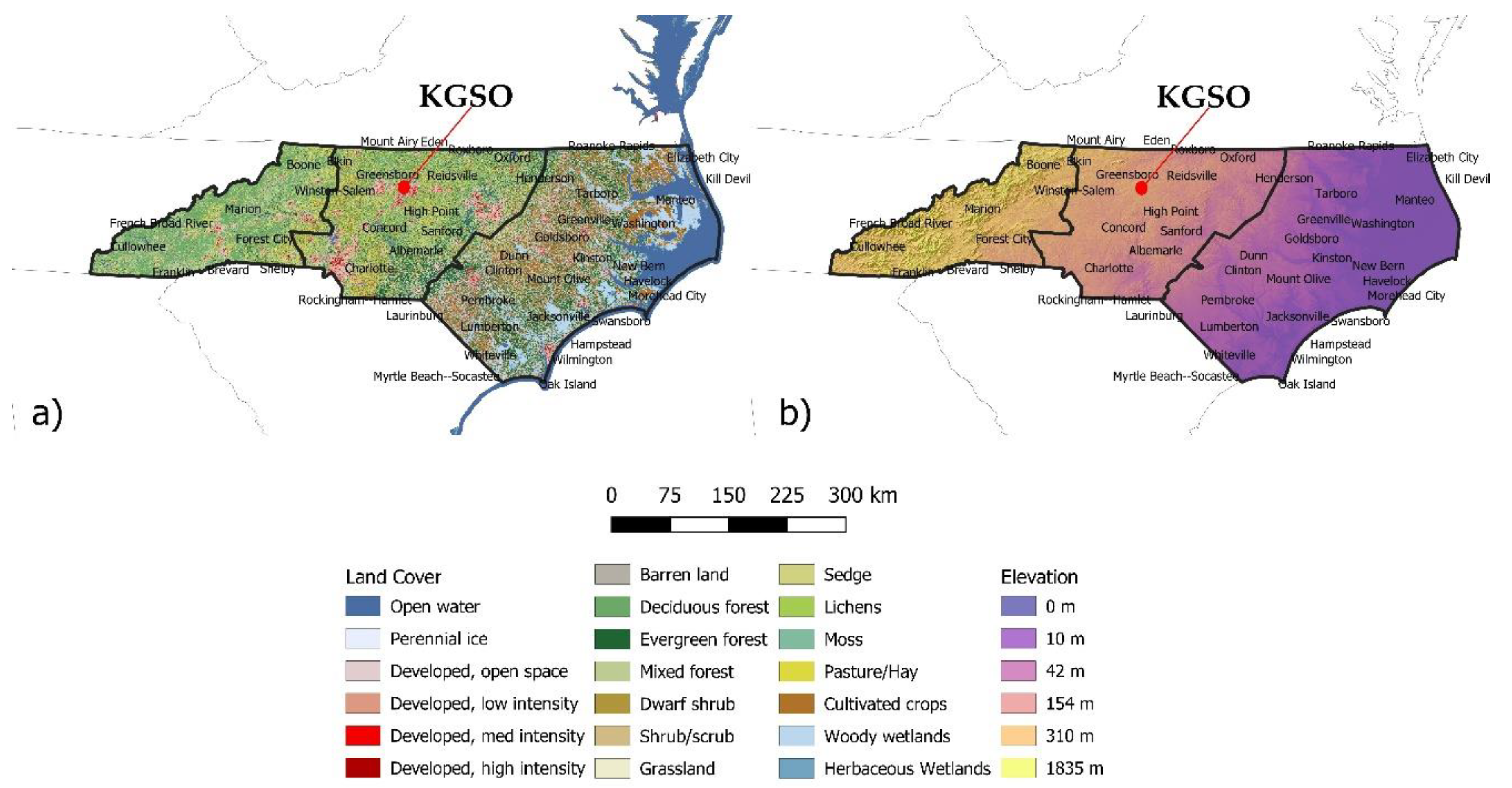
North Carolina offers a unique natural laboratory because it displays a large variety of topographic, soil type, and land use characteristics, including mountainous terrain, dense forests, agricultural lands, metropolitan cities, and low relief coastal regions (Figure 1).

The state is comprised of three geologically distinct regions. Western North Carolina (WNC) is characterized by complex terrain in the Appalachian Mountains covered by a mix of deciduous forests and boreal conifer forests with thick underbrush, as well as a sparse matrix of urban regions. The Piedmont region of central North Carolina (CNC) is a dramatic transition in both vegetation and soil characteristics from the western mountains to the eastern coastal lowlands. CNC transitions from the WNC deciduous and conifer forests to heavy agricultural and urban land cover, and has the highest population density and fastest population growth of the three regions, leading to an increasing trend in impervious surfaces [19,23]. The Coastal Plains in eastern North Carolina (ENC) are characterized by sparsely populated cities, widespread livestock operations, and hardwood swamp forests in the eastern coastal lowlands.

The current study utilized 16 years (2003–2018) of the NCEP Stage IV multi-sensor precipitation estimates product [24]. The NCEP Stage IV product is produced by mosaicking twelve National Weather Service (NWS) River Forecast Center (RFC) hourly Next Generation Weather Radar (NEXRAD) Stage III/Multi-sensor Precipitation Estimator (MPE) products [25]. The Stage III/MPE product is a radar-based precipitation dataset that combines ground and space-derived precipitation estimates and is quality controlled at each RFC. As such, the final Stage IV product produces hourly and daily best estimate gridded precipitation products projected on the Hydrologic Rainfall Analysis Project (HRAP) polar stereographic coordinate system centered at 60° N/105° W with a nominal 4 × 4 km grid resolution. Nelson [26] noted concerns using the hourly estimates due to the automated hourly quality control procedures used at RFCs; therefore, the manually quality controlled daily NCEP Stage IV gridded binary (GRIB I) product was used in the current study.

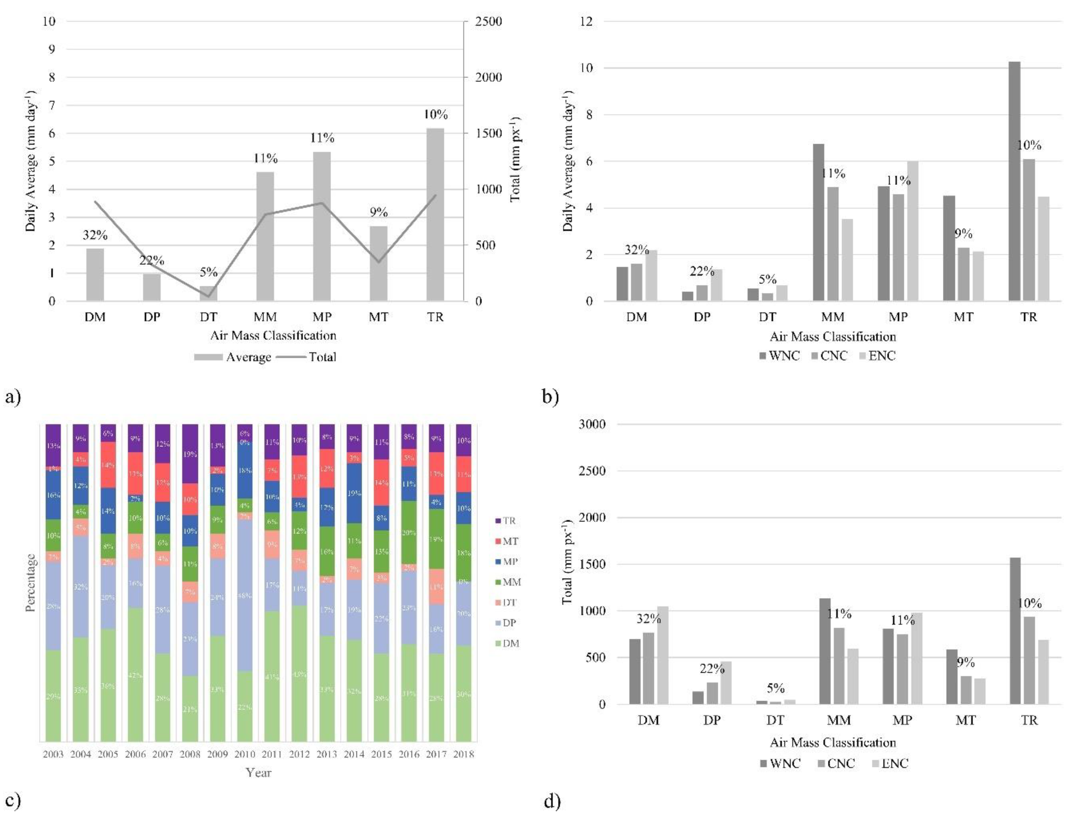
The spatial synoptic classification (SSC) [22] data from the Greensboro station (KGSO) were used to identify the prevailing air mass conditions for each day in the dataset. KGSO was selected because it is a centrally located SSC site in North Carolina and is representative of the prevailing air mass conditions over all three regions. While air mass extents are generally accepted to be larger than the state of North Carolina, it was necessary to justify the viability of using a single, centrally located site. After running a correlation between the Asheville, NC, Greensboro, NC, and Hatteras, NC SSC sites, the results showed moderate agreement. Furthermore, air mass types along the coast would be less variable due to higher station humidity level, while the air mass conditions over the mountains would be highly variable, especially considering the air mass is defined by site specific conditions. As a result, a location in the center of the state was identified as the most representative of the general regional air mass conditions.

Classification of the different air masses by the SSC developed by Sheridan [22] first identified baseline conditions at each site by selecting seed days that described typical meteorological characteristics during each air mass condition, including temperature, dew point depression, mean cloud cover, mean sea level pressure, diurnal temperature range, and diurnal dew point range. With the SSC system, it is possible to classify the prevailing air mass into one of seven categories: transitional (TR), moist tropical (MT), moist moderate (MM), moist polar (MP), dry tropical (DT), dry moderate (DM), and dry polar (DP) (

Table 1. Air mass classification type from the spatial synoptic classification (SSC).

Air Mass	Description
Transitional (TR)	Days with transitioning air mass conditions. Large shifts in pressure, dew point, and wind.
Moist Tropical (MT)	Warm and very humid conditions. Often associated with southerly flow. Typically found in warm sector of mid-latitude cyclones.
Moist Moderate (MM)	Cool and humid conditions. Can form as a modified MP. Can also occur in summer under MT conditions with dense cloud cover.
Moist Polar (MP)	Cool, cloudy, and humid conditions. Typically light precipitation.
Dry Tropical (DT)	Hot, sunny, and dry conditions.
Dry Moderate (DM)	Mild temperatures and dry conditions. Can form when a DP air mass is significantly modified or under periods with zonal flow aloft.
Dry Polar (DP)	Similar to a traditional continental polar (cP) air mass. Often associated with northerly winds. Little to no cloud cover. Advected in by cold-core anticyclones.

). For example, many urban heat island studies focus on MT days because this air mass is typically associated with synoptically benign days that experience conditional instability conducive to thermodynamically driven convection [20,21,22,27]. Additional details on the development of the SSC dataset are provided by Sheridan (http://sheridan.geog.kent.edu/ssc.html, [22]). In the current study, we incorporated all classifications to consider the impact of the prevailing air mass on seasonal spatial and temporal precipitation patterns.

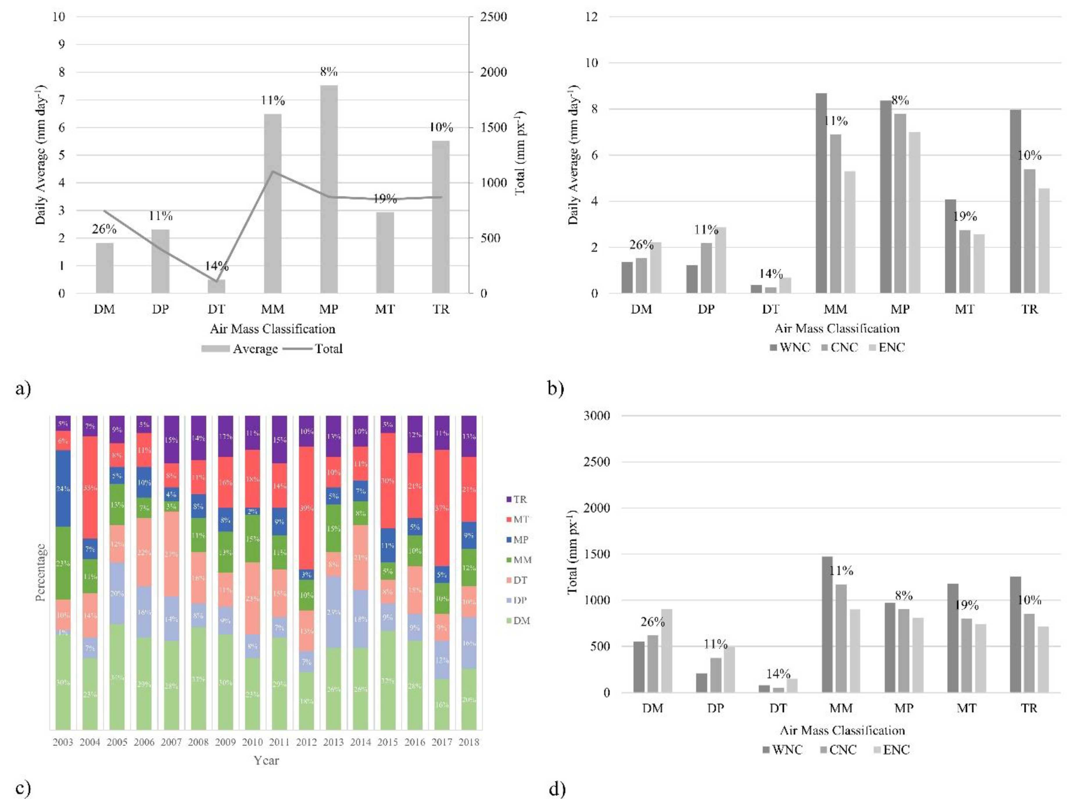
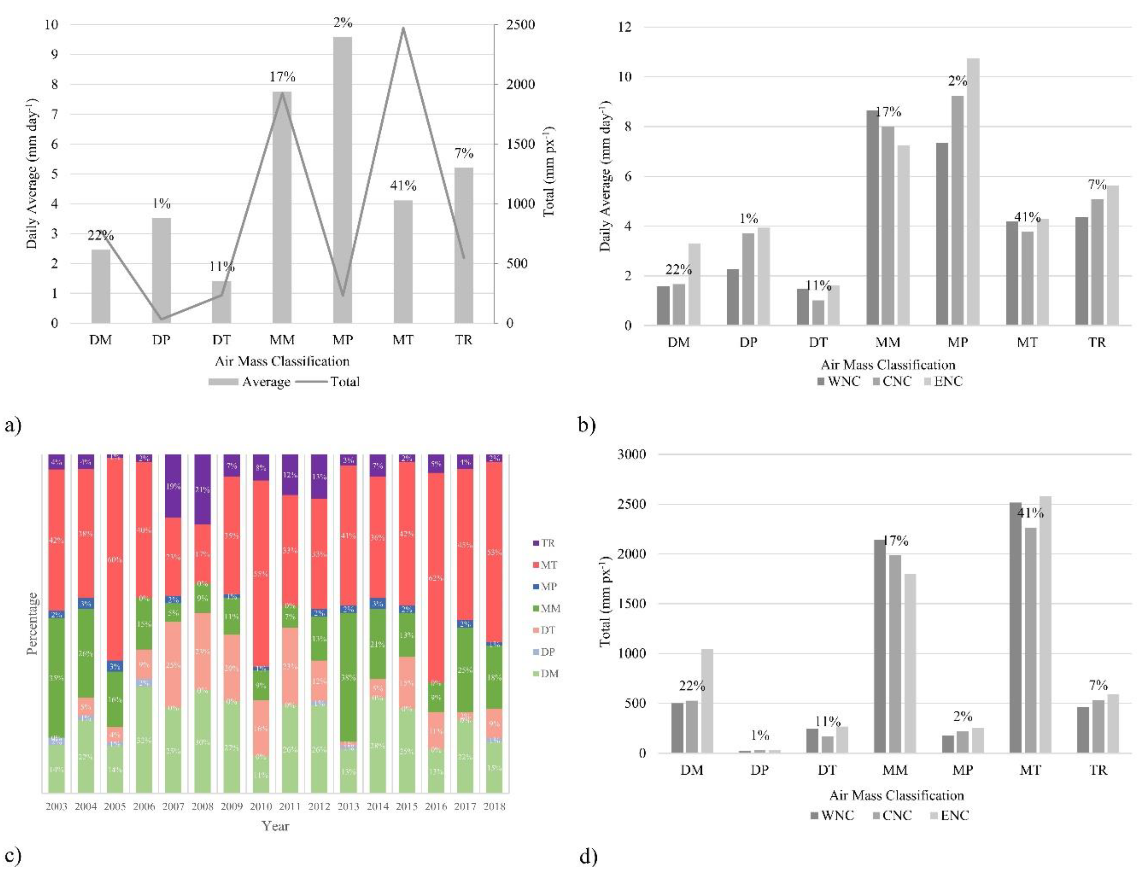
The NCEP Stage IV data were subset seasonally and by air mass. Statewide and regional values were extracted to calculate the daily average and total precipitation within the respective areas. Daily average precipitation represents the average daily precipitation that fell at each pixel contained within the respective area. The total precipitation is presented in units of millimeter per pixel because it represents the total accumulated precipitation averaged across all pixels contained within each respective area. Averaging total precipitation across the respective area rather than adding precipitation accumulation of each grid cell (i.e., pixel) allowed for the comparison of precipitation accumulations between regions by normalizing differences in area. Thus, the daily average provides a rate of precipitation at each pixel, while the total provides the total accumulated precipitation per grid cell for the relative temporal subsets in the study period.

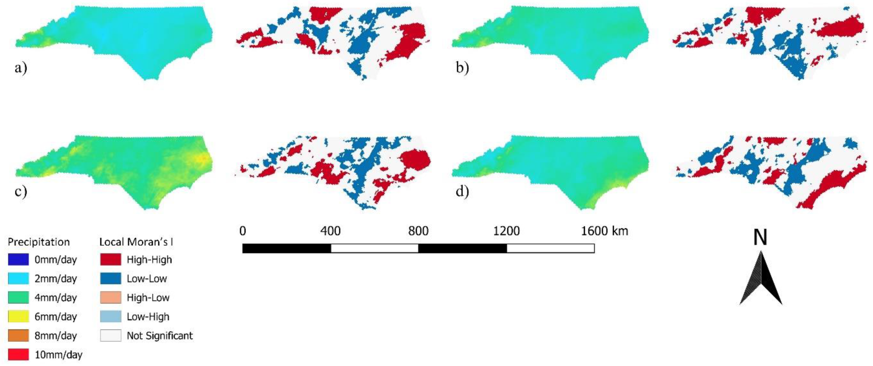
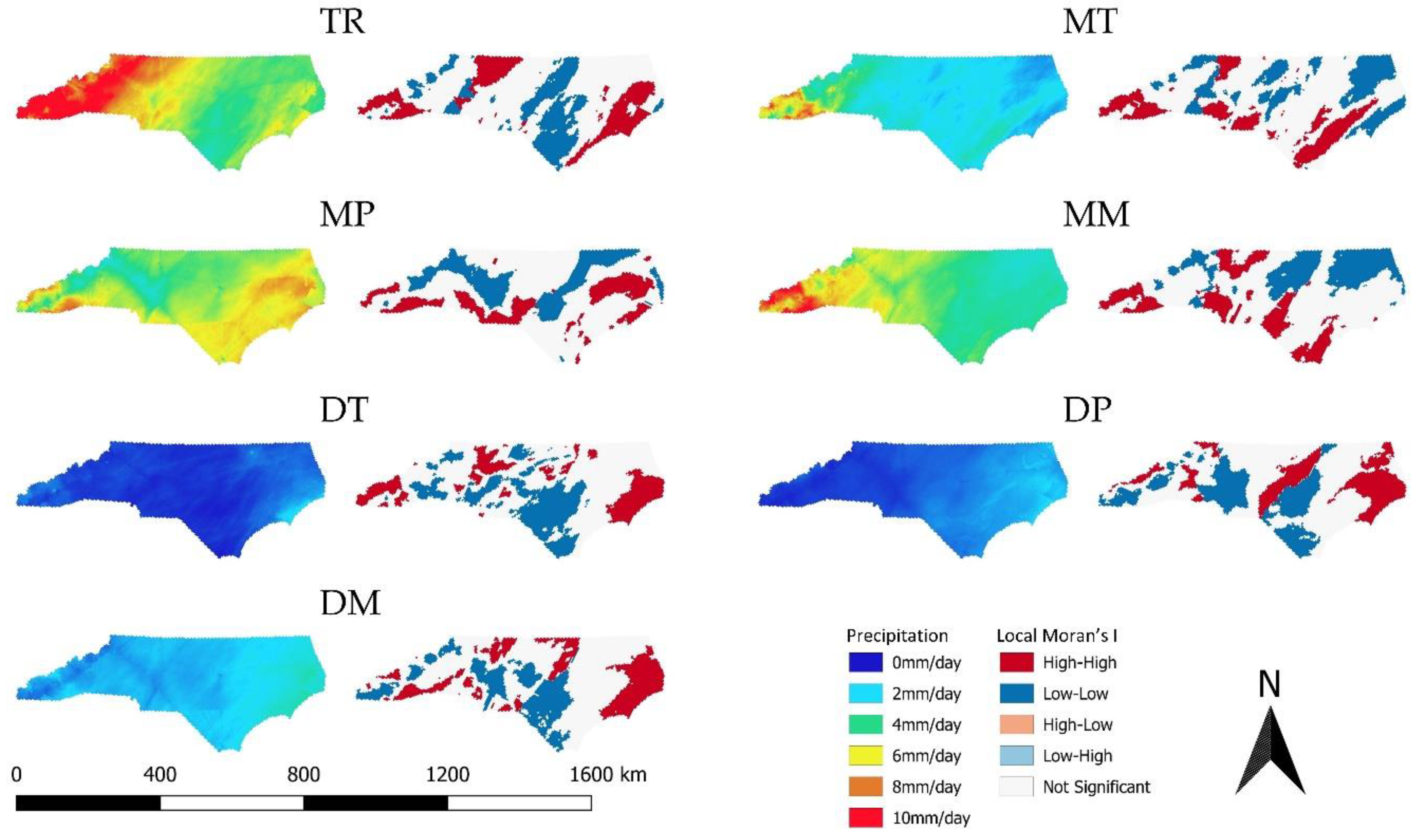
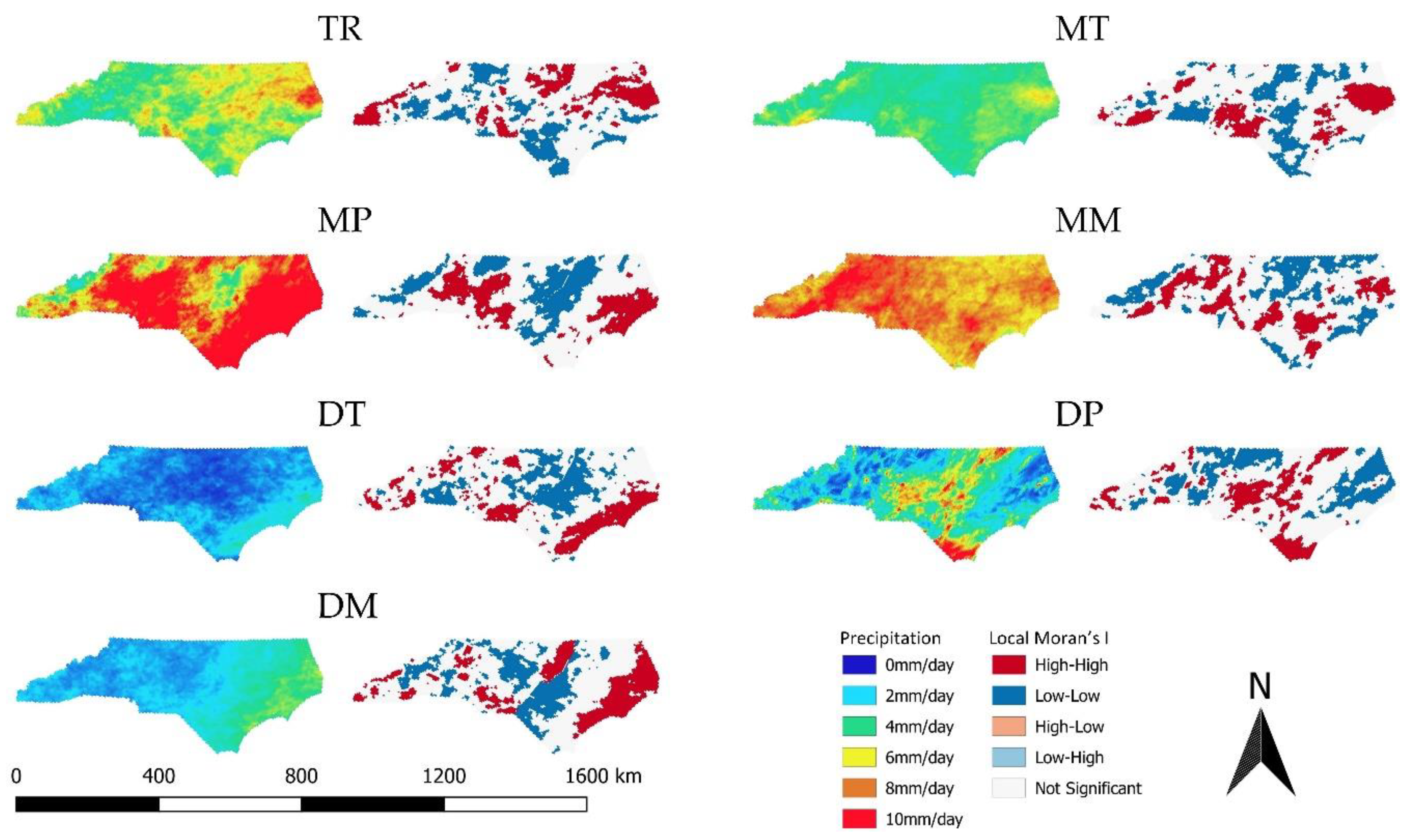
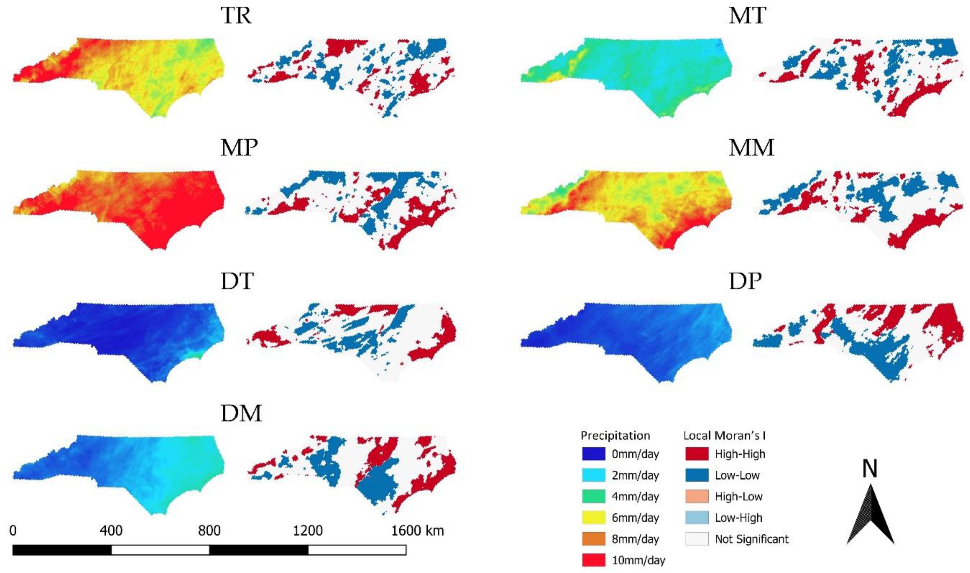
Maps produced from a local indicators of spatial association (LISA) [28] analysis facilitated the assessment of statistically significant high and low precipitation clusters within each of the three North Carolina regions independently. The goal of the LISA analysis was to identify general patterns as reference for forecasters and identify areas of interest for further research. The LISA analysis used the 16-year integrated daily average precipitation for each of the air mass classifications. In this analysis, a local Moran’s I spatial statistic was calculated for each cell based on a queen contiguity spatial neighborhood weight object, and one-sided (alpha = 0.05) hypothesis testing was performed.

In a typical global Moran’s I approach, the Moran’s statistic is structurally similar to a Pearson correlation coefficient, where the Moran’s statistic compares neighboring grid cell z-scores and, if the grid cells have similar values, the term will be positive (i.e., positive spatial autocorrelation) because both grid cells will tend to be either above the sample mean or below the sample mean. However, this global Moran’s I approach only provided information on the general tendency of the dataset to be clustered. Localizing the Moran’s I through the LISA approach instead calculates a Moran’s I statistic and measure of significance at each grid cell. In the current study, this was done by comparing the weighted z-score at each location with the sample mean, which was bounded by each North Carolina geographic region (i.e., WNC, CNC, ENC). This approach was appropriate due to the distinct geological and anthropogenic differences between the three regions. Calculating significance at each grid cell consisted of a Monte Carlo procedure, where actual grid cell values were compared to data values randomly generated and spatially distributed by a permutation procedure. If the observed values exceeded the 95th percentile of the simulated distribution, then it was said to be significant at the 0.05 alpha value. Through this process, statistically significant positive spatial autocorrelation of high values (illustrated as red colors) and low values (illustrated as blue colors) were identified and plotted. Another important outcome from the LISA analysis was the ability to identify outliers. Those were instances when a high (low) value was located in the vicinity of a low (high) value cluster. This produced statistically significant high-low and low-high spatial outliers; however, because the NCEP Stage IV data is a 4 km gridded product quality controlled at each RFC, these outliers were rare. Nonetheless, it was important to include these spatial outlier measures, as it would indicate either unique precipitation conditions or data errors that carried through the quality control procedure.

Furthermore, the LISA analysis was not constrained to adjacent pixels. It was possible to assess the effect of using a decayed distance spatial weighting scheme. This allowed us to address the impact of modifying the neighborhood for each grid cell based on distance from the grid cell of interest. After analyzing the impacts of 8 km, 12 km, 16 km, and 20 km spatial weighting schemes, it was found that 8 km produced the same results as using the applied queen contiguity neighborhood spatial weight. This is due to the fact that at a 4 km grid cell resolution an 8 km spatial weight would only include those pixels adjacent to the grid cell of interest, the same as the queen contiguity. Additional variations to the neighborhood spatial weight of the local Moran’s statistic had little impact on the overall cluster pattern; however, increased spatial weighting distances (e.g., 12 km, 16 km, and 20 km) unrealistically generalized precipitation patterns and eliminated small-scale precipitation clustering characteristics. Specifically, those precipitation clusters analogous with orographic processes were notably lost when neighborhood spatial weights were set too large. It was therefore determined that the queen contiguity neighborhood spatial weight was optimal for the NCEP stage IV 4 km resolution dataset and resolved both homogenous and heterogeneous precipitation events.

3. Results and Discussion

3.1. General Seasonal Patterns

The summer months produced the highest daily average and total rainfall across North Carolina, whereas the winter months had the lowest (Figure 2a). This was consistent within all regions of North Carolina (Figure 2b). However, spatial comparisons of daily average precipitation between regions show that there was a seasonal signal to precipitation maximums across regions (Figure 3). WNC received higher daily average precipitation than CNC and ENC in the winter and spring months, whereas ENC received higher daily average precipitation during the summer and fall months. Spatial patterns followed typical characteristics, where there tended to be a precipitation maximum on the east side of the Appalachian Mountains and along the coastal sandhills (Figure 3). However, this signal was minimized in the winter months (Figure 3a), where precipitation events tended to be driven by northwest flow events after the passage of mid-latitude cyclones. This leads to conditions where the southwestern portion of the Appalachian Mountains observes statistically significant clustering of high daily precipitation amounts. Consistent with Koch and Ray [6], the precipitation maximum over eastern North Carolina is associated with sea breeze circulations that are further enhanced by distinct variations in soil composition.

Spatial precipitation patterns tended to be less consistent across central North Carolina. In the winter and spring months, there was clustering of high precipitation values in the northwest portion of CNC, possibly related to the redevelopment of mesoscale convective systems (MCSs) on the east side of the Appalachian Mountains [5]. In the summer months, this northwest clustering signal was overcome by a region of high precipitation near the Charlotte metropolitan area. It is possible that this is an area of precipitation enhancement downwind of the urban city center, as noted by studies near similar metropolitan areas [17,20,21]; however, there is a need for future research detailing the urban influence on precipitation across North Carolina. The clustering of high precipitation values in the northern portion of CNC and in the southeastern portion of CNC returned in the fall months. This is likely the return of synoptically driven MCS precipitation events propagating eastward across the state.

3.2. Seasonal and Air Mass Precipitation Patterns

It was important to augment the seasonal analysis by focusing on prevailing synoptic-scale air mass conditions to distinguish between synoptically driven and local-scale thermodynamically driven precipitation events within each season. Whereas polar air mass conditions tend to be affiliated with synoptic-scale forcing, moist tropical air mass conditions are commonly used as a proxy for synoptically benign conditions [20,21,22,27]. Also, changes in seasonal air mass frequency may play a role in precipitation distribution and intensity; therefore, it is important to quantify patterns of both air mass type and air mass frequency in documenting seasonal precipitation patterns.

3.2.1. Winter

Winter months are most often characterized by DM and DP air mass conditions (Figure 4a), although while DM and DP dominate the frequency of precipitation and are often associated with the passage of mid-latitude cyclones, MM and MP conditions make substantial contributions to wintertime precipitation totals (~40%). Transitional (TR) air mass conditions also make important contributions to wintertime precipitation. Considering that TR air mass conditions are best described as a blend of the two transitioning air masses, air mass classifications before and after TR days were analyzed to identify the most likely conditions occurring under TR days. In the winter, DM air mass conditions accounted for 35% of days adjacent to TR days, followed by DP (28%), MM (13%), MT (11%), MP (7%), and DT (6%) conditions. Thus, it is possible that DM and DP contributed more to the total precipitation, although TR days may signify unique conditions conducive to high precipitation amounts due to the transitioning of certain air masses, particularly in WNC where the highest daily average and total precipitation occurred during TR air mass conditions (Figure 4b,d). It will be important for future research to further analyze the air masses undergoing transition in conjunction with composite circulations to better understand precipitation forcing under TR days.

Because MP air mass conditions can result from a DP air mass acquiring additional moisture, MP air mass conditions are often associated with the passage of mid-latitude cyclones. MM air mass conditions produce similar conditions to MP, with the exception of having higher temperatures and higher humidity levels. Furthermore, these MM air mass conditions can form independently to the south of MP air masses, for example, when a deep mid-latitude cyclone taps into southerly Gulf moisture. Overall, precipitation totals from DM, DP, MP, and MM air mass conditions made up 68% of total precipitation; 87% after accounting for the precipitation potentially associated with these air masses while undergoing transition during TR days. Regionally, precipitation totals from DM, DP, MP, and MM—including precipitation during the transition of these air masses—made up 82%, 87%, and 89% for WNC, CNC, and ENC, respectively. This is consistent with Nieto-Ferreira et al. [3] who found that 70–80% of total precipitation across North Carolina is associated with the passage of a mid-latitude cyclone, with an increasing gradient from WNC to ENC. Interestingly, the frequency of MM air mass conditions steadily increased from 2010–2018 (Figure 4c). This tends to be at the expense of DP and MP air mass conditions, suggesting that there was a gradual shift to warmer and more humid air mass conditions during the tail-end of the study period (Figure 4c); however, a longer period of record is required to determine if this trend is a significant shift in regional conditions or a regional response to other factors, such as teleconnections.

Spatial precipitation variations support the above assessment, where the highest precipitation totals and significant clustering of high precipitation amounts occurred in the southwest portion and across the southern portion of the study domain under MM conditions (Figure 5). Precipitation totals tended to be most homogenous during DT, DP, and DM air mass conditions, where there was a gradual west-to-east increasing gradient in daily average precipitation across North Carolina. Furthermore, areas with significant clustering of high precipitation amounts under dry air mass conditions tended to cluster across the northern portion of the study domain, suggesting that these events originated poleward of the study domain. The highest rain amounts in ENC were associated with MP events. In addition, the enhanced clustering of high precipitation amounts in the southern portion of the domain during MP and MM supports the possibility that these air mass conditions result from the northward advection of Gulf moisture during the passage of mid-latitude cyclones.

3.2.2. Spring

The springtime distribution of air mass conditions was similar to the winter; however, there was a decrease in the frequency of DM and DP air mass days and an increase in the number of MT and DT days (Figure 6). Similar to the winter months, TR days were most often associated with DM air mass conditions (30%); however, there was a notable increase in the number of TR days associated with DT (18%) and MT (17%) days at the expense of DP (19%) and MP (4%) days. This is consistent with the expected transition from a strong synoptic winter regime toward the relatively weak synoptic summer regime [3]. There was a notable shift to more intense precipitation conditions across all three regions (Figure 6b). Thus, there was an affiliated increased risk of hazardous hydrometeorological events due to the shift to air mass conditions conducive to high intensity precipitation events.

While dry air mass conditions maintained significant clustering of high precipitation toward the northern portion of North Carolina, moist air mass conditions no longer had a southern tendency in the clustering of high precipitation amounts (Figure 7). MT springtime days were characterized by a northern distribution of high precipitation clustering; however, the clusters were more localized and sporadic for all moist air mass regimes, suggesting a shift toward thermodynamically driven precipitation events and enhanced connectivity between land cover conditions and precipitation. This is an important consideration because it also appears from visual inspection that there was an increased percentage of MT days during spring months over the study period (Figure 6c). This comes at the expense of fewer DM, DP, and DT days, suggesting a shift to more humid springtime air mass conditions conducive to thermodynamically driven precipitation events.

3.2.3. Summer

There was an abrupt increase in daily average rainfall in the summer months and a shift to a higher frequency of synoptically benign MT days (Figure 8). These MT days made up 41% of the daily summertime air mass regimes, followed by DM, MM, DT, TR, MP, and DP; however, DM days neighbored TR days 30% of the time, with MT days accounting for 29%. DT days combined for 21% of days adjacent to TR days followed by MM conditions (16%). DP and MP combined to contribute only 4% of days adjacent to TR days. While there were a limited number of days subject to MP air mass conditions (2%), these air mass conditions were conducive to intense precipitation events (Figure 8b and Figure 9). Also notable was the substantial contributions to total precipitation from MM air mass conditions. While MM days made up only 17% of summertime days, they contributed the second largest amount to total precipitation (31%, Figure 8b). Unlike the winter and spring, there was no clear visual shift in the frequency of air mass conditions over the period of study (Figure 8c).

The spatial patterns of summer precipitation exhibited a heterogeneous distribution of precipitation across North Carolina (Figure 9). There was significant clustering in the Coastal Plains, but the previously strong clustering in the southwest Appalachian Mountains weakened, and precipitation appears to have been heavily impacted by local-scale orographic processes in western North Carolina. Under the majority of summertime air mass conditions, there was significant clustering near the urbanized Triad (i.e., Winston-Salem, Greensboro, High Point) region in CNC. It has been documented that population growth and urbanization across the CNC have contributed to increasing trends in urban heat island signatures [19]. As observed around other metropolitan areas [17,20,21], it is possible that the pockets of significant precipitation clustering in CNC are associated with local-scale thermodynamic forcing and land cover boundaries, which prompts a need for future research to assess the influence of land cover on precipitation across North Carolina.

3.2.4. Fall

Fall is indicative of a shift away from synoptically benign conditions in the summer to the typical strong synoptic-scale forcing in the winter (Figure 10). There was a shift from MT air mass conditions to a higher frequency of MP and DM air mass conditions. While the signal in statewide daily average and total precipitation was similar to the spring months, fall is unique in that daily average precipitation in ENC during MM and MP days was greater than WNC (Figure 10b). This is likely related to an increase in mid-latitude cyclone activity coinciding with antecedent summertime patterns favorable for moisture advection. Fall months exhibited a large decrease in the percentage of DT days (9%) adjacent to TR days; a value closer to what was found in wintertime DT days (6%). As in all seasons, DM days (36%) were most often adjacent to TR days, followed by DP (21%), MM (16%), MT (14%), and MP (4%) days.

Similar to the spring months, there was a notable increase in the percentage of days under MT tropical air mass conditions from 2010–2018 (Figure 10c). This is an important outcome because it appears the transitional and winter month air mass conditions were becoming warmer and more humid over the period of the study. A spatial pattern that distinguishes the fall from the spring months is an area of high precipitation amounts clustered over the southeast portions of the domain (Figure 11). Under MT conditions, this is most likely associated with the passage of tropical cyclones, whereas the southeastern clustering during DT and DM are likely associated with the passage of mid-latitude cyclones, sea breeze circulations, or a combination of both.

4. Conclusions

The current study used 16 years (2003–2018) of the National Center of Environmental Prediction (NCEP) Stage IV precipitation dataset to characterize the impact of air mass conditions on seasonal precipitation patterns in North Carolina. Results from the current study aid forecasting and mitigation of hydrometeorological hazards in North Carolina by documenting the spatial and temporal patterns of precipitation magnitude in the context of prevailing air mass conditions. It was found that winter is dominated by dry moderate (DM) and dry polar (DP) air mass conditions indicative of synoptically driven precipitation events. Spatial clustering confirms this conclusion, where there tends to be clustering of high precipitation amounts on the east side of the Appalachian Mountains and along the Coastal Plains. With an increased number of moist tropical (MT) and dry tropical (DT) days, springtime illustrated a shift from synoptically driven precipitation events to weak synoptic forcing conditions, leading to a greater influence of topography and thermodynamically driven events. North Carolina experienced more heterogeneous and higher daily average precipitation amounts in the spring than winter months. Summertime precipitation was more heterogeneous due to prevailing MT air mass conditions indicating a tendency towards localized and more intense thermodynamically driven precipitation events. Furthermore, it was discovered that while moist moderate (MM) and moist polar (MP) air mass conditions were less frequent, they exhibited the highest daily average rainfall rates, suggesting that MM and MP air mass conditions are conducive to hazardous hydrometeorological events. While high humidity levels in the fall maintained high daily precipitation totals under moist air mass conditions, there was a return to wintertime characteristics, as the percentage of DP and DM days had a notable increase. In addition, the heterogeneous summertime precipitation spatial distribution began to give way to spatial patterns more similar to the winter months.

With the patterns identified in the current study, future research should use the spatial clustering outcomes to identify and examine areas where small-scale clustering of high precipitation amounts coincides with local-scale variations in land cover conditions. In addition, there is a need to understand the magnitude of correlations between air mass conditions and large-scale teleconnections. This analysis should include an investigation of composite circulations associated with each air mass to characterize the synoptic and mesoscale processes associated with each air mass classification in the Southeast United States. A notable result of this study was that winter, spring, and fall months exhibited a shift to warmer and more humid MM and MT air mass conditions over the 2003–2018 study period. This shift could lead to more thermodynamically driven and more intense precipitation events, especially during the spring and fall transitional seasons; however, a longer period of record in addition to air mass trend analyses across North Carolina is needed to assess the significance of these tendencies.

References

1. Seto, K.C.; Shepherd, J.M. Global urban land-use trends and climate impacts. Curr. Opin. Environ. Sustain. 2009, 1, 89–95. [Google Scholar] [CrossRef]
2. Bureau, U.C. Fastest-Growing Cities Primarily in the South and West. Available online: https://www.census.gov/newsroom/press-releases/2019/subcounty-population-estimates.html (accessed on 14 August 2019).
3. Ferreira, R.N.; Hall, L.; Rickenbach, T.M. A climatology of the structure, evolution, and propagation of midlatitude cyclones in the southeast united states. J. Clim. 2013, 26, 8406–8421. [Google Scholar] [CrossRef]
4. Shepherd, J.M.; Grundstein, A.; Mote, T.L. Quantifying the contribution of tropical cyclones to extreme rainfall along the coastal southeastern United States. Geophys. Res. Lett. 2007, 34, 1–5. [Google Scholar] [CrossRef]
5. Parker, M.D.; Ahijevych, D.A. Convective Episodes in the East-Central United States. Mon. Weather Rev. 2007, 135, 3707–3727. [Google Scholar] [CrossRef]
6. Koch, S.E.; Ray, C.A. Mesoanalysis of Summertime Convergence Zones in Central and Eastern North Carolina. Weather Forecast. 1997, 12, 56–77. [Google Scholar] [CrossRef]
7. Dyer, J. Analysis of a Warm-Season Surface-Influenced Mesoscale Convective Boundary in Northwest Mississippi. J. Hydrometeorol. 2011, 12, 1007–1023. [Google Scholar] [CrossRef]
8. Boyles, R.P.; Raman, S. Analysis of climate trends in North Carolina (1949–1998). Environ. Int. 2003, 29, 263–275. [Google Scholar] [CrossRef]
9. Sayemuzzaman, M.; Jha, M.K. Seasonal and annual precipitation time series trend analysis in North Carolina, United States. Atmos. Res. 2014, 137, 183–194. [Google Scholar] [CrossRef]
10. Shepherd, J.M.; Burian, S.J. Detection of Urban-Induced Rainfall Anomalies in a Major Coastal City. Earth Interact. 2003, 7, 1–17. [Google Scholar] [CrossRef] [Green Version]
11. Krajewski, W.F.; Ciach, G.J.; Habib, E. An analysis of small-scale rainfall variability in different climatic regimes. Hydrol. Sci. J. 2003, 48, 151–162. [Google Scholar] [CrossRef] [Green Version]
12. Parker, M.D.; Knievel, J.C. Do meteorologists suppress-thunderstorms? Radar-derived statistics and the behavior of moist convection. Bull. Am. Meteorol. Soc. 2005, 86, 341–358. [Google Scholar] [CrossRef]
13. Dyer, J.L.; Garza, R.C. A Comparison of Precipitation Estimation Techniques over Lake Okeechobee, Florida. Weather Forecast. 2004, 19, 1029–1043. [Google Scholar] [CrossRef]
14. Dyer, J. Evaluation of Surface and Radar-Estimated Precipitation Data Sources Over the Lower Mississippi River Alluvial Plain. Phys. Geogr. 2009, 30, 430–452. [Google Scholar] [CrossRef]
15. Stevenson, S.N.; Schumacher, R.S.; Stevenson, S.N.; Schumacher, R.S. A 10-Year Survey of Extreme Rainfall Events in the Central and Eastern United States Using Gridded Multisensor Precipitation Analyses. Mon. Weather Rev. 2014, 142, 3147–3162. [Google Scholar] [CrossRef]
16. Moore, B.J.; Mahoney, K.M.; Sukovich, E.M.; Cifelli, R.; Hamill, T.M.; Moore, B.J.; Mahoney, K.M.; Sukovich, E.M.; Cifelli, R.; Hamill, T.M. Climatology and Environmental Characteristics of Extreme Precipitation Events in the Southeastern United States. Mon. Weather Rev. 2015, 143, 718–741. [Google Scholar] [CrossRef]
17. Dixon, P.G.; Mote, T.L. Patterns and Causes of Atlanta’s Urban Heat Island–Initiated Precipitation. J. Appl. Meteorol. 2003, 42, 1273–1284. [Google Scholar] [CrossRef]
18. Rickenbach, T.M.; Nieto-Ferreira, R.; Zarzar, C.; Nelson, B. A seasonal and diurnal climatology of precipitation organization in the southeastern United States. Q. J. R. Meteorol. Soc. 2015, 141, 1938–1956. [Google Scholar] [CrossRef]
19. Doran, E.M.B.; Golden, J.S. Climate & Sustainability Implications of Land Use Alterations in an Urbanizing Region: Raleigh-Durham, North Carolina. J. Environ. Prot. (Irvine, Calif). 2015, 07, 1072–1088. [Google Scholar]
20. Ashley, W.S.; Bentley, M.L.; Stallins, J.A. Urban-induced thunderstorm modification in the Southeast United States. Clim. Change. 2012, 113, 481–498. [Google Scholar] [CrossRef]
21. Haberlie, A.M.; Ashley, W.S.; Pingel, T.J. The effect of urbanisation on the climatology of thunderstorm initiation. Q. J. R. Meteorol. Soc. 2015, 141, 663–675. [Google Scholar] [CrossRef]
22. Sheridan, S.C. The redevelopment of a weather-type classification scheme for North America. Int. J. Climatol. 2002, 22, 51–68. [Google Scholar] [CrossRef]
23. Tippett, R. NC Demographic Trends Through 2035 House Select Committee on Strategic Transportation Planning and Long Term Funding Solutions. In Proceedings of the House Select Committee on Strategic Transportation Planning and Long Term Funding Solutions, Chapel Hill, NC, USA, 22 February 2016; Available online: https://www.ncleg.gov/documentsites/committees/house2015-172/2-22-16_Meeting/Demographic_Trends_through_2035.pdf (accessed on 14 August 2019).
24. Cooperative Distributed Interactive Atmospheric Catalog System/Earth Observing Laboratory/National Center for Atmospheric Research/University Corporation for Atmospheric Research, and C.P.C.C. for E.P.W.S.S.D. of C. NCEP/CPC Four Kilometer Precipitation Set, Gauge and Radar. Available online: https://doi.org/10.5065/D69Z93M3 (accessed on 19 September 2019).
25. Lin, Y.; Mitchell, K.E. The NCEP stage II/IV hourly precipitation analyses: Development and applications. In Proceedings of the 19th Conf. Hydrology, San Diego, CA, USA, 9–13 January 2005. [Google Scholar]
26. Nelson, B.R.; Prat, O.P.; Seo, D.-J.; Habib, E. Assessment and Implications of NCEP Stage IV Quantitative Precipitation Estimates for Product Intercomparisons. Weather Forecast. 2016, 31, 371–394. [Google Scholar] [CrossRef]
27. Mote, T.L.; Lacke, M.C.; Shepherd, J.M. Radar signatures of the urban effect on precipitation distribution: A case study for Atlanta, Georgia. Geophys. Res. Lett. 2007, 34, 2–5. [Google Scholar] [CrossRef]
28. Anselin, L. Local Indicators of Spatial Association—LISA. Geogr. Anal. 1995, 27, 93–115. [Google Scholar] [CrossRef]
Figure 1. (a) National Land Cover Database (NLCD) 2016 data and (b) elevation. Three regions are delineated from left to right as western North Carolina, central North Carolina, and eastern North Carolina. Air mass conditions were determined from the Greensboro (KGSO) spatial synoptic classification site.
Atmosphere 10 00624 g001
Figure 2. (a) Statewide precipitation daily average and total precipitation and (b) regional assessment of daily average precipitation for western North Carolina (WNC), central North Carolina (CNC), and eastern North Carolina (ENC). Totals are presented as millimeters per pixel (mm px−1), which is equivalent to millimeters per grid cell.
Atmosphere 10 00624 g002
Figure 3. Daily average precipitation (left) and spatial clustering analysis of precipitation (right) for winter (DJF) (a), spring (MAM) (b), summer (JJA) (c), and fall (SON) (d) over the 2003–2018 study period. Local Moran’s I was calculated within each region individually.
Atmosphere 10 00624 g003
Figure 4. (a) winter (DJF) statewide daily average precipitation and total precipitation for each SSC air mass classification; (b) daily average precipitation for each North Carolina region; (c) frequency of each SSC air mass classification over the study period; (d) total precipitation for each North Carolina region. Percentages indicate the fraction of air mass classification for each season (a,b,d) or year (c). Totals are presented as millimeters per pixel (mm px−1), which is equivalent to millimeters per grid cell.
Atmosphere 10 00624 g004
Figure 5. Winter (DJF) daily average precipitation (left) and spatial clustering analysis of precipitation (right) for each SSC air mass classification.
Atmosphere 10 00624 g005
Figure 6. (a) spring (MAM) statewide daily average precipitation and total precipitation for each SSC air mass classification; (b) daily average precipitation for each North Carolina region; (c) frequency of each SSC air mass classification over the study period; (d) total precipitation for each North Carolina region. Percentages indicate the fraction of air mass classification for each season (a,b,d) or year (c). Totals are presented as millimeters per pixel (mm px−1), which is equivalent to millimeters per grid cell.
Atmosphere 10 00624 g006
Figure 7. Spring (MAM) daily average precipitation (left) and spatial clustering analysis of precipitation (right) for each SSC air mass classification.
Atmosphere 10 00624 g007
Figure 8. (a) summer (JJA) statewide daily average precipitation and total precipitation for each SSC air mass classification; (b) daily average precipitation for each North Carolina region; (c) frequency of each SSC air mass classification over the study period; (d) total precipitation for each North Carolina region. Percentages indicate the fraction of air mass classification for each season (a,b,d) or year (c). Totals are presented as millimeters per pixel (mm px−1), which is equivalent to millimeters per grid cell.
Atmosphere 10 00624 g008
Figure 9. Summer (JJA) daily average precipitation (left) and spatial clustering analysis of precipitation (right) for each SSC air mass classification.
Atmosphere 10 00624 g009
Figure 10. (a) fall (SON) statewide daily average precipitation and total precipitation for each SSC air mass classification; (b) daily average precipitation for each North Carolina region; (c) frequency of each SSC air mass classification over the study period; (d) total precipitation for each North Carolina region. Percentages indicate the fraction of air mass classification for each season (a,b,d) or year (c). Totals are presented as millimeters per pixel (mm px−1), which is equivalent to millimeters per grid cell.
Atmosphere 10 00624 g010
Figure 11. Fall (SON) daily average precipitation (left) and spatial clustering analysis of precipitation (right) for each SSC air mass classification.
Atmosphere 10 00624 g011