Article

A Method for Estimating Annual Cumulative Soil/Ecosystem Respiration and CH4 Flux from Sporadic Data Collected Using the Chamber Method

1
Key Laboratory of Ecosystem Network Observation and Modeling, Institute of Geographic Sciences and Natural Resources Research, Chinese Academy of Sciences, Beijing 100101, China
2
College of Resources and Environment, University of Chinese Academy of Sciences, Beijing 100049, China
3
School of Geosciences, The University of Edinburgh, Edinburgh EH9 3FF, UK
4
Co-Innovation Center for Sustainable Forestry in Southern China, College of Biology and the Environment, Nanjing Forestry University, Nanjing 21003, China
*
Authors to whom correspondence should be addressed.
Atmosphere 2019, 10(10), 623; https://doi.org/10.3390/atmos10100623
Submission received: 21 July 2019 / Revised: 25 September 2019 / Accepted: 12 October 2019 / Published: 16 October 2019
(This article belongs to the Special Issue Biogenic Emissions to the Atmosphere)

Abstract

:
Measurements of greenhouse gas fluxes over many ecosystems have been made as part of the attempt to quantify global carbon and nitrogen cycles. In particular, annual flux observations are of great value for regional flux assessments, as well as model development and optimization. The chamber method is a popular approach for soil/ecosystem respiration and CH4 flux observations of terrestrial ecosystems. However, in situ flux chamber measurements are usually made with non-continuous sampling. To date, efficient methods for the application of such sporadic data to upscale temporally and obtain annual cumulative fluxes have not yet been determined. To address this issue, we tested the adequacy of non-continuous sampling using multi-source data aggregation. We collected 330 site-years monthly soil/ecosystem respiration and 154 site-years monthly CH4 flux data in China, all obtained using the chamber method. The data were randomly divided into a training group and verification group. Fluxes of all possible sampling months of a year, i.e., 4094 different month combinations were used to obtain the annual cumulative flux. The results showed a good linear relationship between the monthly flux and the annual cumulative flux. The flux obtained during the warm season from May to October generally played a more important role in annual flux estimations, as compared to other months. An independent verification analysis showed that the monthly flux of 1 to 4 months explained up to 67%, 89%, 94%, and 97% of the variability of the annual cumulative soil/ecosystem respiration and 92%, 99%, 99%, and 99% of the variability of the annual cumulative CH4 flux. This study supports the use of chamber-observed sporadic flux data, which remains the most commonly-used method for annual flux estimating. The flux estimation method used in this study can be used as a guide for designing sampling programs with the intention of estimating the annual cumulative flux.

1. Introduction

CO2 and CH4 fluxes from and to terrestrial ecosystems are important to quantify as they influence the atmospheric greenhouse gas concentrations and thus climate warming [1,2]. Terrestrial ecosystems have a global annual soil respiration of approximately 90 Pg C yr−1 [3,4]. Methane has a global warming potential 34 times that of CO2 for a period of over 100 years [5], and the terrestrial CH4 flux can be large when the methanotrophic process is constrained by moisture and temperature [6]. Methane emission is currently estimated at 500–600 Tg CH4 yr−1 globally [7]. Ground observations of soil/ecosystem respiration and CH4 fluxes have increased considerably over the past few decades [8], driven by the need to adapt to, and mitigate, climate change. Among them, the chamber method is one of the most common methods to observe fluxes and to understand their spatial and temporal variations [9].
The chamber method has been applied since the early twentieth century and has a history of use of nearly one hundred years [10]; the method is relatively easy, cheap, and widely applicable to varied environments [9]. There are currently at least 5000 sampling plots worldwide [9]. However, until very recently, the chamber method was essentially manually controlled, and thus had the disadvantage of a low observation frequency and inconsistent sampling months. In recent years, this limitation has been largely overcome by the introduction of computer-controlled automatic sampling systems [11,12]. However, the automatic equipment is usually expensive to install, although increasingly more studies have started to use this new efficient system [13,14,15,16,17]. Thus, for the archived data now available, the observation frequency is often less than once a month, determined according to the practicability of accessing the site, and usually in the daytime. Here, we examine archived flux data of CO2 and CH4 collected in China at 2096 and 1331 sampling locations respectively. Among these, only 249 and 105 sampling plots were observed as frequently as monthly. We ask whether the less-frequent data may be regarded as representative of the year as a whole.
The annual flux value is expressed as the cumulative flux (AF) or average flux ( A F ¯ ) during one year and represents a portion of the important basic data for carbon budgets [18]. Simulation of annual flux using machine learning approaches and process-based models are powerful and promising methods in filling flux observation gaps spatially or temporally [19,20,21]. However, all these methods depend on data availability of the predictors, which commonly are remotely sensed and meteorological gridded data. Those data contain biases and gaps that lead to an increase of predictive uncertainty [22,23,24]. Besides, some anthropogenic influences are hard to be quantified in models, for example management practice or disturbance. Therefore cross-validation and fusion of multiple originated data are necessary for producing a confident global flux map, including a wide variety of modeled and observed data sets. As we mentioned previously, a large number of chamber-observed data are collected sporadically. If those data could confidently be used to estimate the annual flux, the value of the archived data could be increased considerably. Some previous studies have indeed attempted to estimate the annual value using flux data derived from different seasons using arithmetic averaging or weighted averaging for a single plot or a few plots [25,26]. The two algorithms have the advantages of simple calculation and easy implementation, which is preferable for constructing universal annual estimation equations for different ecosystems.
In view of the above-mentioned problems and needs, in this study we focus on multi-source data collection; the objectives are to (1) analyze the relationships between the observed flux in different months and the observed AF to test the feasibility of using low-frequency flux data to estimate the overall AF; (2) select the optimal months for AF estimation using different observation frequencies and determine the optimal equations for AF estimation. The results of the present study provide guidance for AF estimations using archived low-frequency flux data and for future design of sampling programs.

2. Methods

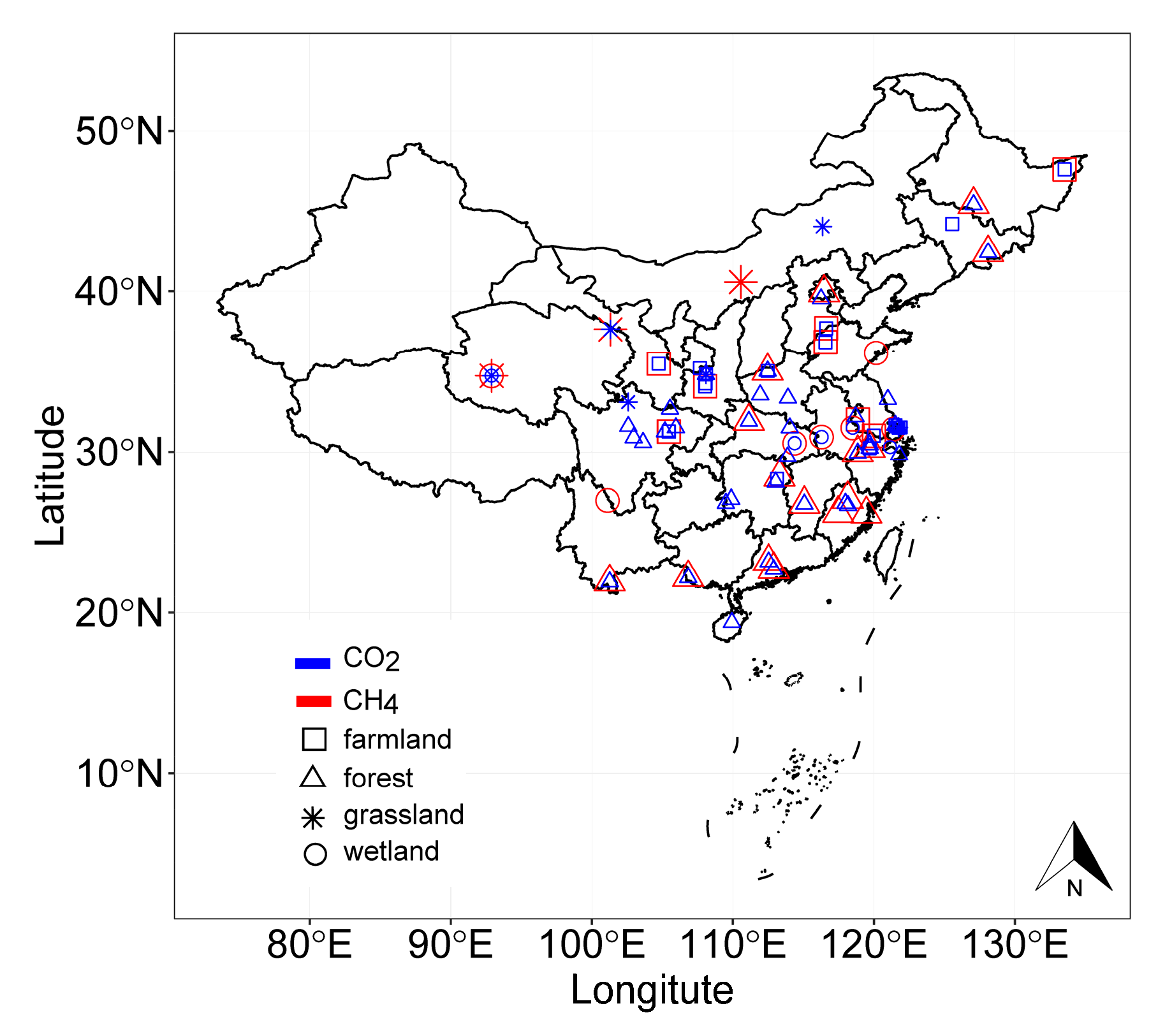
2.1. Data Collection and Screening

We began this research with the preparation of the monthly flux data from Chinese data archives. Using the China National Knowledge Infrastructure (CNKI) database, we first collected related research literature published up to 2016 and extracted soil CO2 and CH4 flux data using the GetData Graph Digitizer software (version 2.25, GetData Software). The criteria for the data selection were: (1) in situ monitoring; (2) using the chamber method, including self-made chambers and commercial products; (3) a study duration of at least 12 months with at least one campaign per month. All three criteria were required for the data set to qualify for the study. Following the screening, 65 valid research articles were obtained, including 245 soil/ecosystem respiration sampling plots and 96 CH4 flux sampling plots. The duration of some observation programs was more than 1 year. We selected just the period covering 12 months from the start of the first campaign. The remaining months, shorter than 1 year, were abandoned. This resulted in 283 groups of 1-year monthly soil/ecosystem respiration data and 107 groups for the CH4 data.
In addition to the literature data, we acquired chamber-observed in situ flux data for 10 sites from a research project (Carbon Budget in Terrestrial and Marginal Sea Ecosystems of China [27]) covering these locations: Haibei, Sanjiang, Yucheng, Yanting, Wuxi, Changbai Mountain, Dinghushan, Heshan, Qianyanzhou, and Xishuangbanna. We obtained 47 groups of 1-year monthly flux data for CO2 and CH4.
In total, we collected 330 groups of 1-year monthly soil/ecosystem respiration data and 154 groups for the CH4 data. Ecosystem net CO2 exchange (NEE) data was not used in the present study because achieved chamber NEE data is limited. More information on the collected data is illustrated in Figure 1 and Table 1.

2.2. Development and Testing of AF Estimation Equations

The purpose of this study is to determine if it is possible to estimate the AF using infrequent observation data, while evaluating the performance of different sampling months as predictors of AF. Raw flux data expressed in seconds or hours was first converted into monthly and annual flux data. Subsequently, we developed linear regressions using the observed monthly flux of the sample month or months as the predictor variable and the observed AF as the response variable. The validation data, which were not used in the equation development, were used to evaluate the performance of the equations. A detailed explanation of the methods is as follows.

2.2.1. Data Preparation for the Development and Testing of the Equations for Annual Soil/Ecosystem Respiration and CH4 Cumulative Fluxes (AFCO2 and AFCH4): Observed Monthly Cumulative Flux Calculations

We assumed that one or more observations in a month can represent the cumulative monthly flux (MF). The raw flux data were partitioned by month. The simple arithmetic mean F ¯ (mg m−2 h−1) of each month’s flux and the monthly cumulative flux (g m−2 month−1), was then calculated. MF was used to denote the observed monthly flux, as shown in the subsequent section.

2.2.2. Data Preparation for the Development and Testing of the AFCO2 and AFCH4 Equations: Observed AF Calculations

The observed annual flux was obtained by accumulating the MF over 12 months:
A F o b s = 1 12 M F ,  
where AFobs is the observed annual value (g m−2 yr−1).
The dataset was then randomly divided into two groups by site-year following previous studies [3,28,29], i.e., 2/3 of the site-years and resulting AFobs were used as training data to develop the estimation equations and the remaining 1/3 of the site-years were used as validation data to test the estimation accuracy of the equations.

2.2.3. Development of the Estimation Equations for AFCO2 and AFCH4

Linear regression equations were developed for the subsequent AF simulation using the observed MF of each month or of a combination of months as the candidate predictor variable and the observed AF as the response variable. We developed two types of AF estimation equations, i.e., the AF estimation method I (AFI, Equation (2)), based on the arithmetic average and the AF estimation method II (AFII, Equation (3)), based on the weighted average method, as follows:
AFI : A F sim = a + α M F ¯ ,  
where AFsim (g m−2 yr−1) is the simulated AF, a is the intercept, α is the regression coefficient, and M F ¯ (g m−2 month−1) is the average of the observed MF over one or more months. In order to comprehensively evaluate the simulative ability of different sampling months, we used an exhaustive method including every possible combination of the sampling months. For example, at a sampling frequency of one, there were 12 potential sampling times. At a frequency of two, any combination of two months was possible, i.e., there were 66 potential sampling times. Similarly, at frequencies of 3 to 11, there were 220, 495, 792, 924, 792, 495, 220, 66, and 12 potential combinations, respectively. In total, we developed and compared 4094 equations for the AF estimation using the arithmetic average method.
The weighted average method requires a weighting coefficient for each month:
AFII : A F sim = a + α M F 1 + β M F 2 + + λ M F n ,
where AFsim is the simulated AF (g m−2 yr−1), a is the intercept, α, β and λ are regression coefficients representing the weighting factors, and MF1, MF2 and MFn (g m−2 month−1) indicate the monthly flux of January, February, and the n month, respectively. As with the AFI, we also used an exhaustive method for the AFII and analyzed 4094 AF estimation equations based on the weighted average method.

2.2.4. Testing the Estimation Accuracy of the Equations

We used the verification group of the observed flux data and all the equations to calculate the AFsim. To assess the accuracy of the simulation, the R2 values of the linear relationship between the AFobs and AFsim and the root mean square error (RMSE) were determined and used as indicators. Lower values of RMSE indicated a better performance in the predictions.

2.2.5. Comparison of Estimating Accuracies of Different Ecosystem Types and Interface Types

Considering the small sample size, we were not able to perform a sampling period comparison, nor were we able to determine predictive equations for different ecosystems (e.g., forest, grassland, farmland and wetland) and different interfaces (i.e., ecosystem, soil and water, which correspond to different flux component, including ecosystem respiration, soil respiration, heterotrophic respiration, CH4 flux of soil, and CH4 flux of soil and plant). Thus, we separately accessed the simulative accuracy. The result of the testing of the four optimal equations (minimum RMSE) are plotted for the sampling frequencies of 1 to 4. For equations with a higher sampling frequency, a greater estimation accuracy was generally observed. More information could be found in Tables S1–S4.

2.2.6. Testing the Present Annual Flux Estimation Method with Eddy Covariance Data

Due to the lack of continuous flux data observed with chamber technique, eddy covariance data was used to implement a further validation of the present method. We obtained continuous half-hour flux data (ecosystem respiration, RECO) of 26 site-years of 10 sites in China from FLUXNET (Data Products: FLUXNET2015 Dataset, [30]). The basic information of the sites was shown in Table 2.
Using every site-year data, the optimal equation with sampling frequencies of 4 (i.e., Equation (B4) in Table 3) was tested as an example. Four random RECO data were selected in May, July, September and December (one datum for each month, data only selected from 8 a.m. to 6 p.m. to keep the time consistent with the practice of the manual chamber technique). The simulated annual RECO was then derived using the 4 random respirations and the recommended Equation (B4). The random data selection and annual RECO simulation was repeated 100 times. The observed annual RECO was derived by accumulating the half-hour respirations of a year.
The simulated annual RECO was compared to the observed annual RECO. The R2 and root mean square error (RMSE) values between the observed and simulated annual RECO were used to assess the accuracy of the predictive equation.

2.3. Statistical Analysis

Statistical analysis was performed using the software R, version 3.4.4 [31], with the ‘broom’ [32], ‘dplyr’ [33] and ‘boot’ [34] packages. The simulative performances of the two types equations AFI and AFII were compared using a paired t-test. The correlation matrix was plotted using the R package ‘PerformanceAnalytics’ [35], with Spearman method. Figures were plot using the R packages ‘ggplot2’ [36], ‘ggpubr’ [37] and ‘grid’ [31], and SigmaPlot (version 11.0, SYSTAT, USA).

3. Results

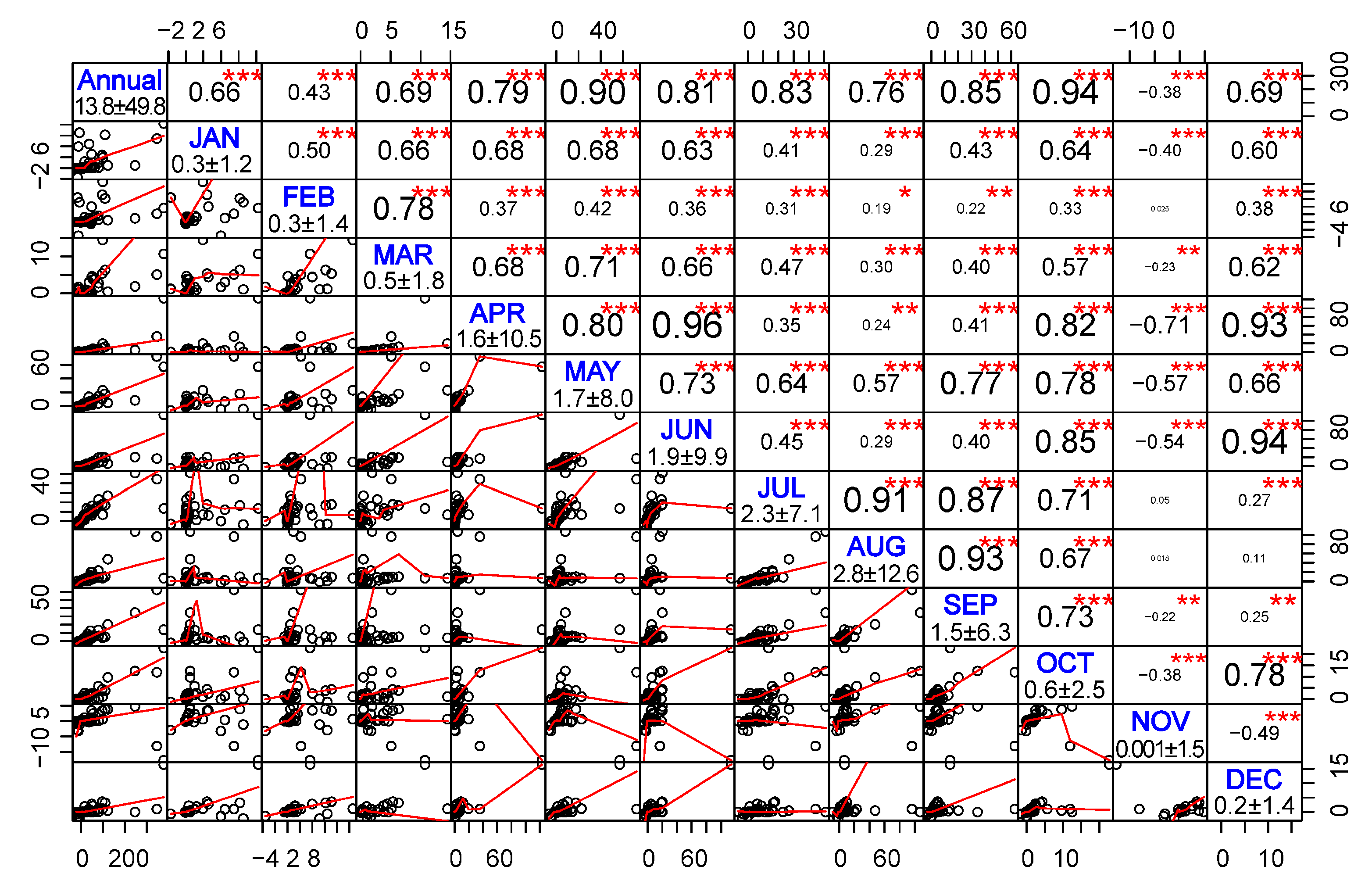
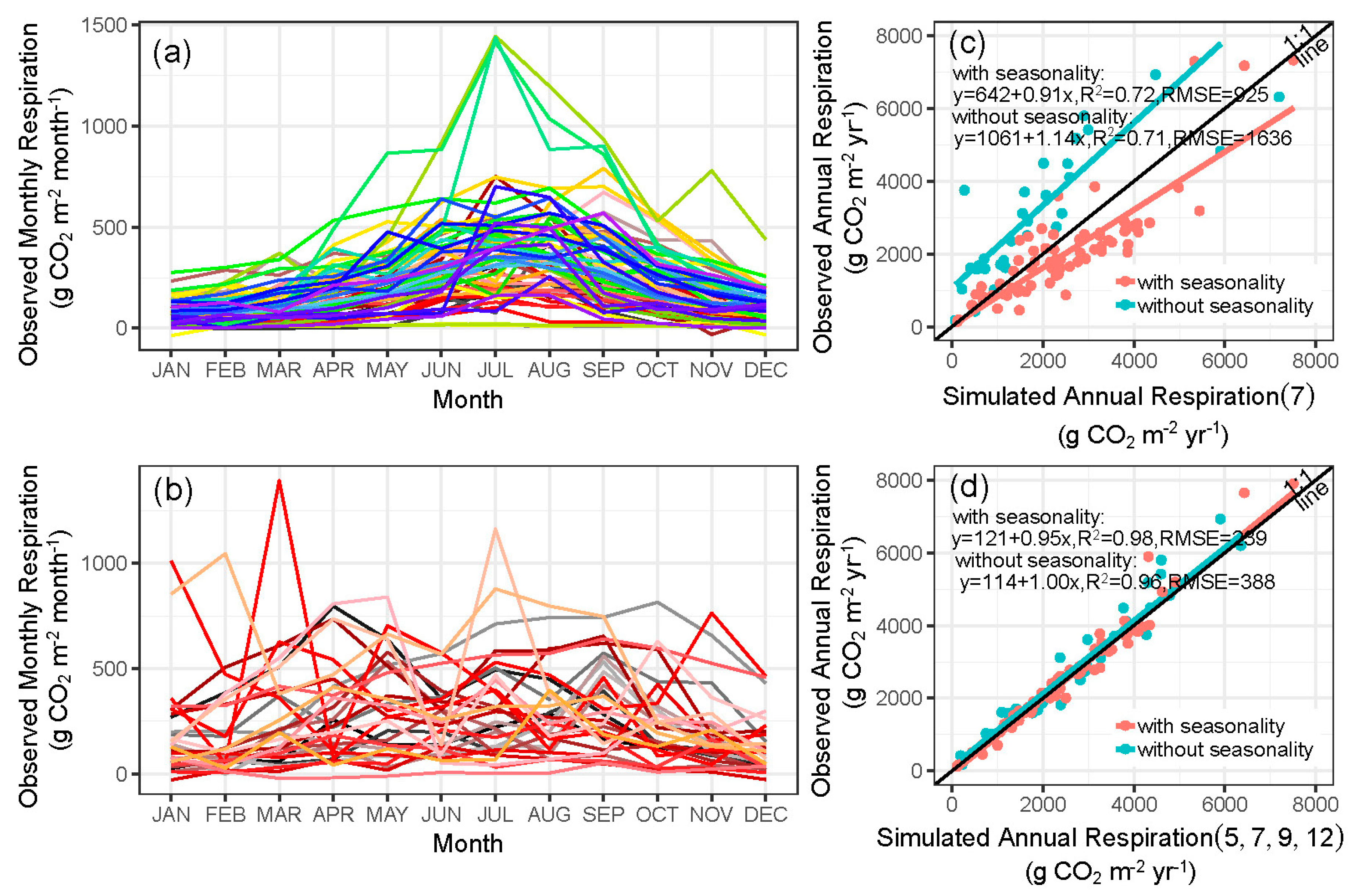
3.1. Relationships between Observed Annual and Monthly Flux

The observed CO2 monthly emissions were highly correlated with observed AF. The correlation coefficients (r value) ranged from 0.71 to 0.92 (p < 0.001, Figure 2). The monthly emissions of the warm period, e.g., from May to September, exhibited particularly high correlations (r > 0.9) with AF. Observed CH4 monthly fluxes were also significantly correlated with AF (p < 0.001), yet r values varied from −0.38 to 0.94 (Figure 3). The correlation coefficients of the months from April to October (r values between 0.76–0.94) were higher than that of the colder period from November to March (r values between −0.38–0.69).

3.2. Comparison of Different Types of Equations

Using the developed equations and the flux data validation group, we obtained the simulated AF and compared it to the observed AF. Taking the R2 and RMSE values of the test data, the performance of different types of equations, AFI and AFII, were compared.
For both soil/ecosystem respiration and CH4 flux prediction, AFI and AFII produced similar R2 and RMSE value and trends, particularly in terms of the mean R2, maximum R2, mean RMSE and minimum RMSE (Figure 4). Although there were the similar values and trends, a significant difference was observed. The simulation error of the AFII equation was significantly lower (CO2: p < 0.001, df = 4093; CH4: p < 0.001, df = 4093) than that of AFI equation. The average RMSE values were 462 ± 3 g CO2 m−2 yr−1 and 14.3 ± 0.18 g CH4 m−2 yr−1 for AFII, 490 ± 3 g CO2 m−2 yr−1 and 16.0 ± 0.18 g CH4 m−2 yr−1 for AFI. When the amount of monthly flux was fixed from 1 to 11, for the most cases, the minimum RMSE of the AFII equation was smaller than that of AFI equation (Figure 4). Because of the high similarity of AFI and AFII equations, in the remaining results sections (Section 3, Section 4 and Section 5), only results of AFII are presented.

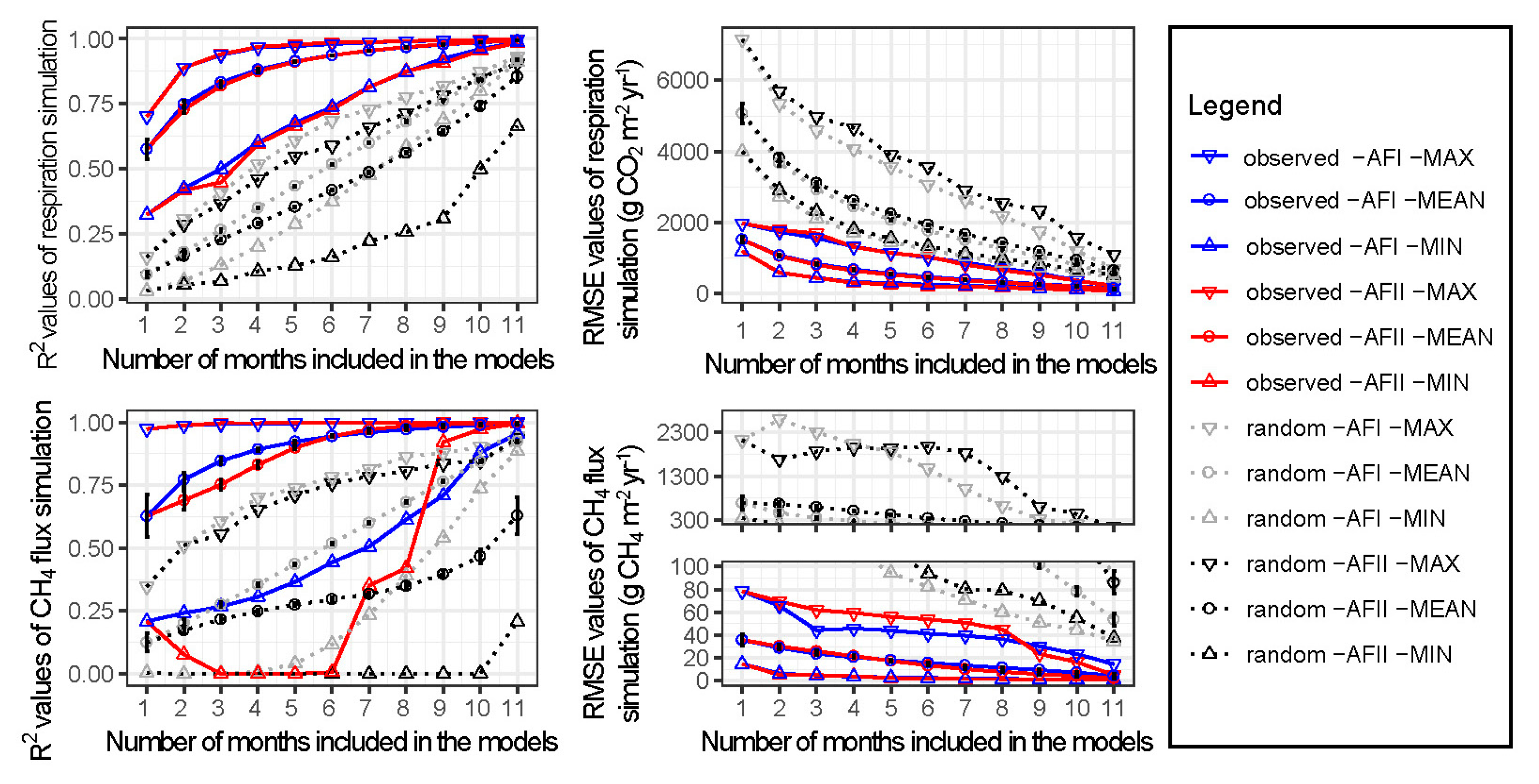
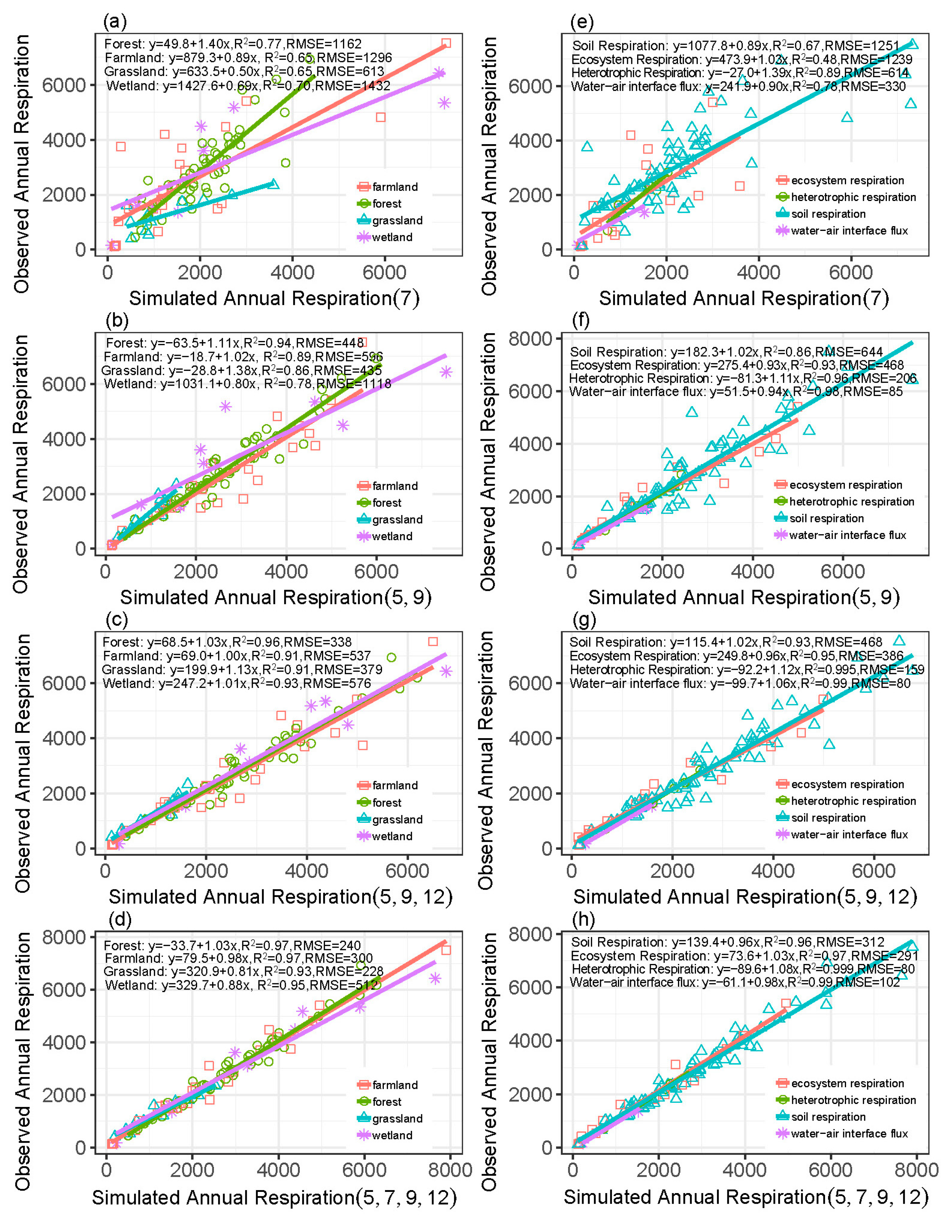
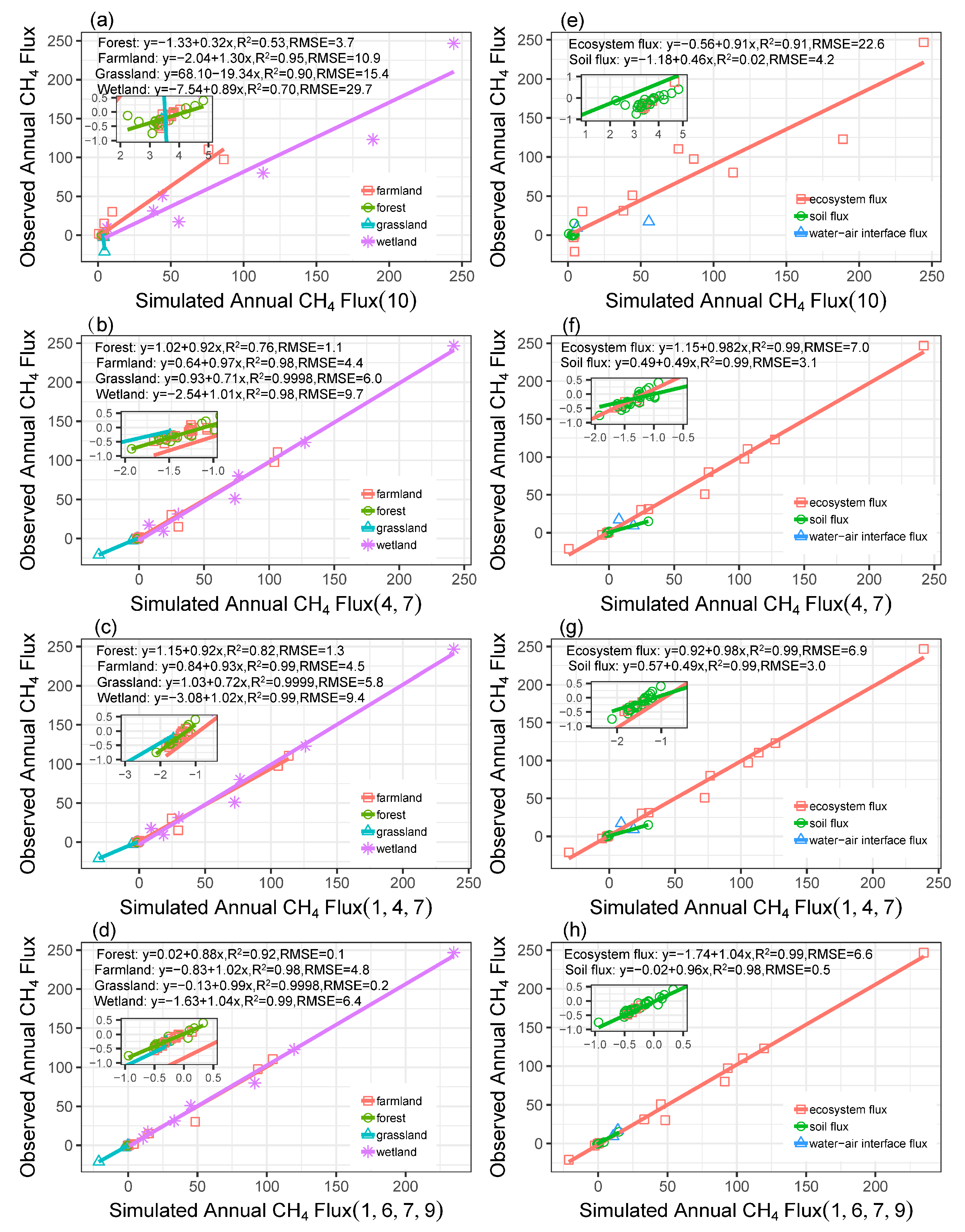
3.3. Effects of Sampling Frequency on AF Estimation

To analyze the effects of the sampling frequency (the number of sampling months per year) on the AF estimation, taking the flux values of 1 to 11 months as predictors, we compared the agreement between the simulated AF and the observed AF of the test dataset, using the R2 and RMSE values.
As the sampling frequency increased, the agreement between the AFobs and AFsim (R2 value) increased, while the estimating error (RMSE value) decreased (Figure 4).
When estimating the AFCO2 and AFCH4 using only the flux from one month, the variability was explained, on average, by 58% and 63%, respectively (Figure 4). Increasing the sampling frequency caused a gradual improvement in the consistency. For estimations of AFCO2 and AFCH4 using 2 to 4 months of flux data, the explained variabilities increased from 73% to 88% and from 69% to 83%, respectively. Moreover, the mean RMSE declined from 1051 ± 30 to 637 ± 8 g CO2 m−2 yr−1 for AFCO2 and from 30.1 ± 1.9 to 21.7 ± 0.6 g CH4 m−2 yr−1 for AFCH4.
When the focus was only placed on the optimal equations, the emission of one to four months could explain AFCO2 variation at 70%, 89%, 94% and 97% respectively. Moreover, the simulation errors were 1186, 584, 431 and 292 g CO2 m−2 yr−1, respectively (Table 3). For AFCH4 simulation, only one month’s flux could explain 97% variation. When using the flux from two months, the explanation increased to 99%, with an error of 5.2 g CH4 m−2 yr−1.
As the sampling frequency increased to more than 4 times per year, the rate of change in the R2 and RMSE value, particularly in terms of maximum R2 and minimum RMSE value, decreased.

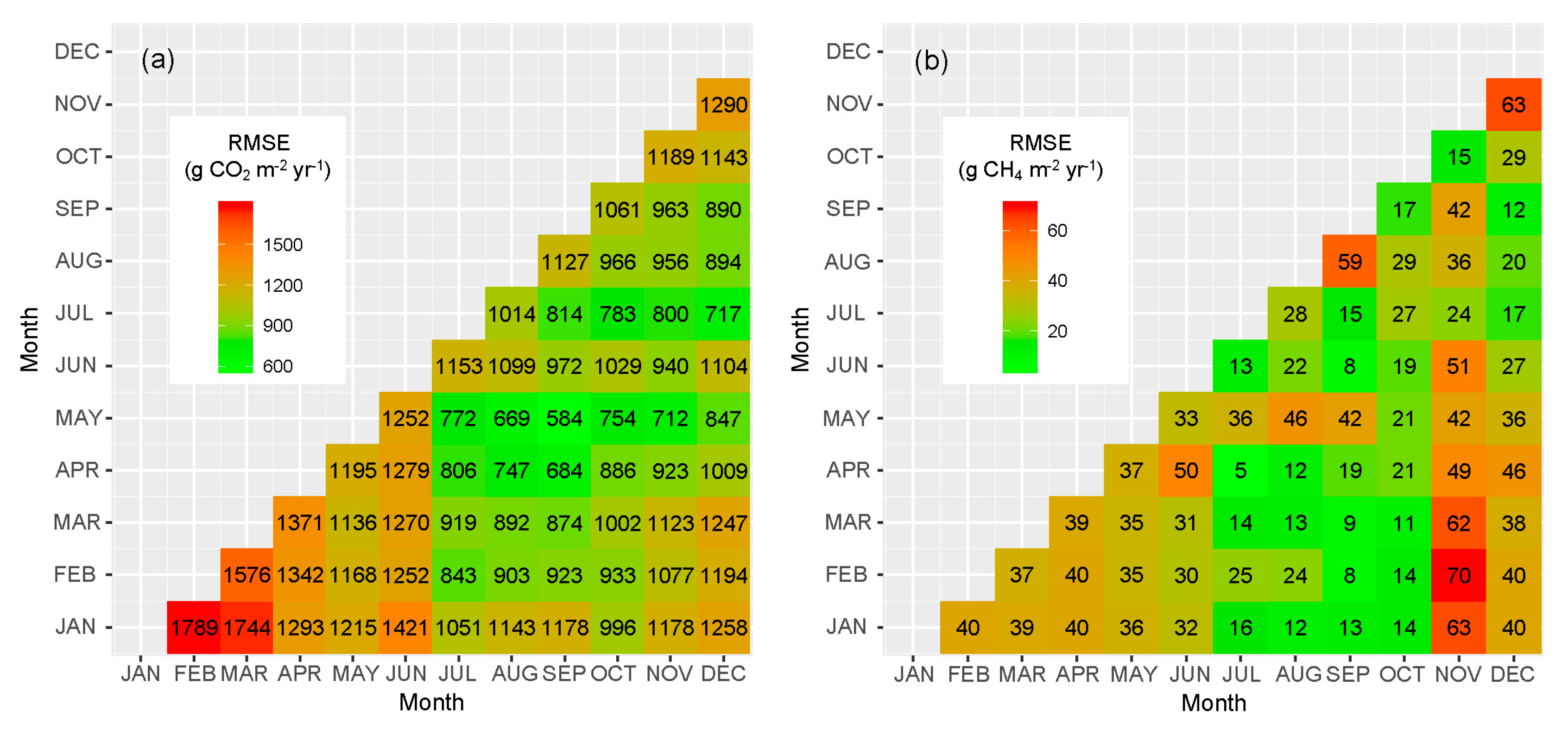
3.4. Effects of Sampling Months on AF Estimation

Using the R2 and RMSE of test dataset, the influence of specific sampling months on the AF estimation was compared.
Results showed that when the sampling frequency was too low to cover different seasons, the simulation accuracy was generally better when the flux of May to October was used compared to months of November to April. When one month was used for the AFCO2 simulations, the first six minimum RMSE values were obtained using the respirations of July, September, May, October, November and August (Table S2). For the AFCH4 simulation, the fluxes of October, September, July, June, August and May demonstrated a greater prediction performance (Table S4). When two months were used in AFCO2 and AFCH4 simulation, the predictive errors were always large if the two monthly fluxes were both from November to April (Figure 5).
Although increasing sampling frequency could generally improve simulation accuracy as described in the previous section (Result Section 3), observations in the period from May to October demonstrated a higher prediction performance than more-frequent observations in the period from November to April. For example, the R2 and RMSE of one month of July (Equation (B1), Table 3) were 0.67 and 1186 g CO2 m−2 yr−1, respectively. This indicates a better performance than for the four cold months of January, February, March, and April, whose R2 and RMSE were 0.60 and 1306 g CO2 m−2 yr−1, respectively (Equation (W4), Table 3). However, it should be noted that when there was more than one sampling month, the R2 was higher if the flux data was derived from different seasons but not all from the warm period (Table 3, Tables S1–S4).

3.5. Simulative Accuracies of Different Ecosystem Types and Interface Types

The simulative accuracies of different ecosystem types were generally distinct (Figure 6 and Figure 7). Estimations of AFCO2 and AFCH4 of forest and grassland exhibited a smaller RMSE compared to other ecosystems, indicating a higher simulation accuracy. In contrast, the estimation of the wetland ecosystem demonstrated the lowest accuracy. However, results also showed that the more months used in the prediction, the smaller the difference in terms of estimating accuracy among different types of ecosystem (i.e., the smaller the difference in R2 and RMSE values). Similarly, the discrepancy of estimation accuracies among different interfaces also decreased when more monthly fluxes were included into estimations. When 4 monthly fluxes were used in AF simulation, there was no big discrepancy in terms of R2 values among different ecosystem types and interface types.

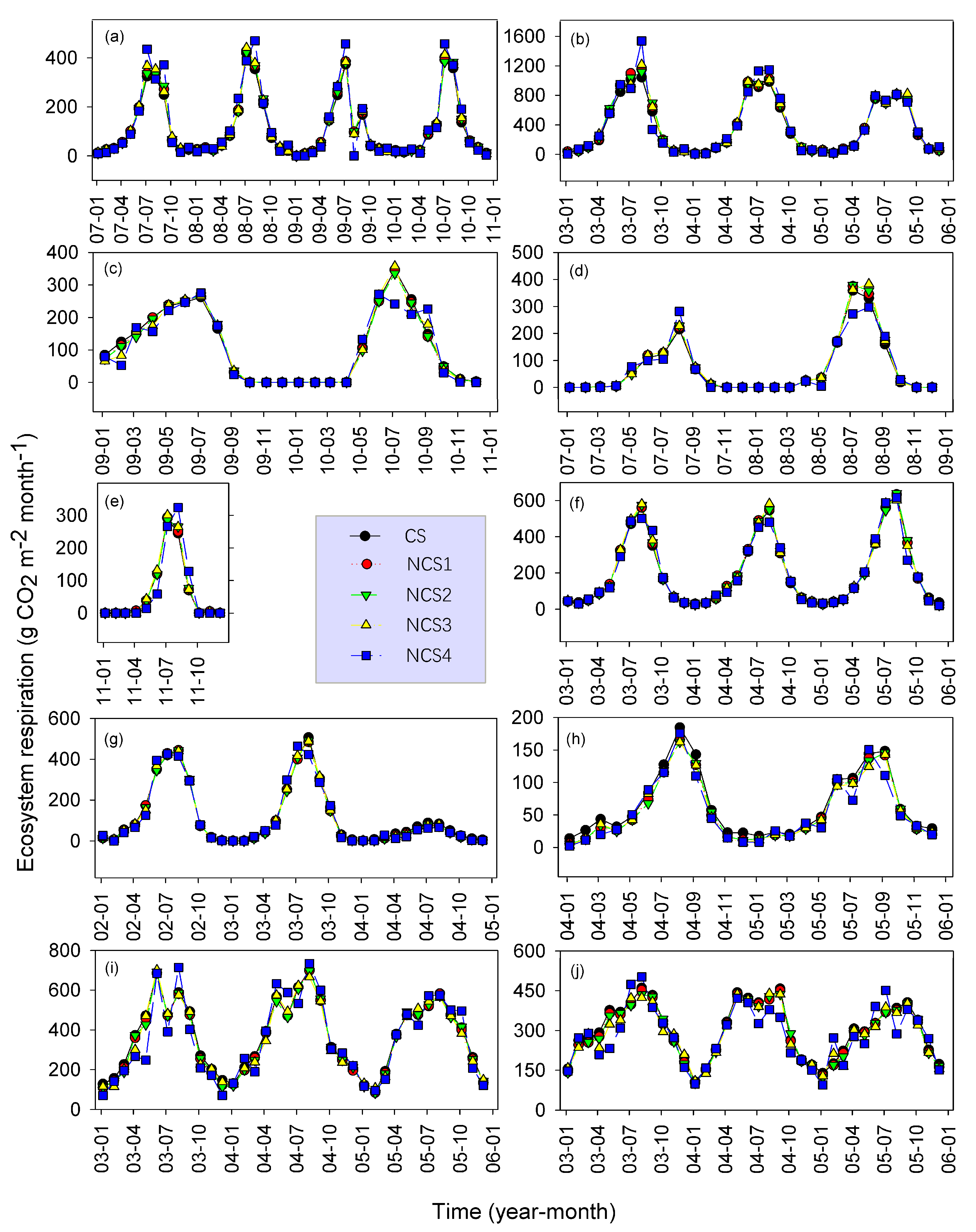
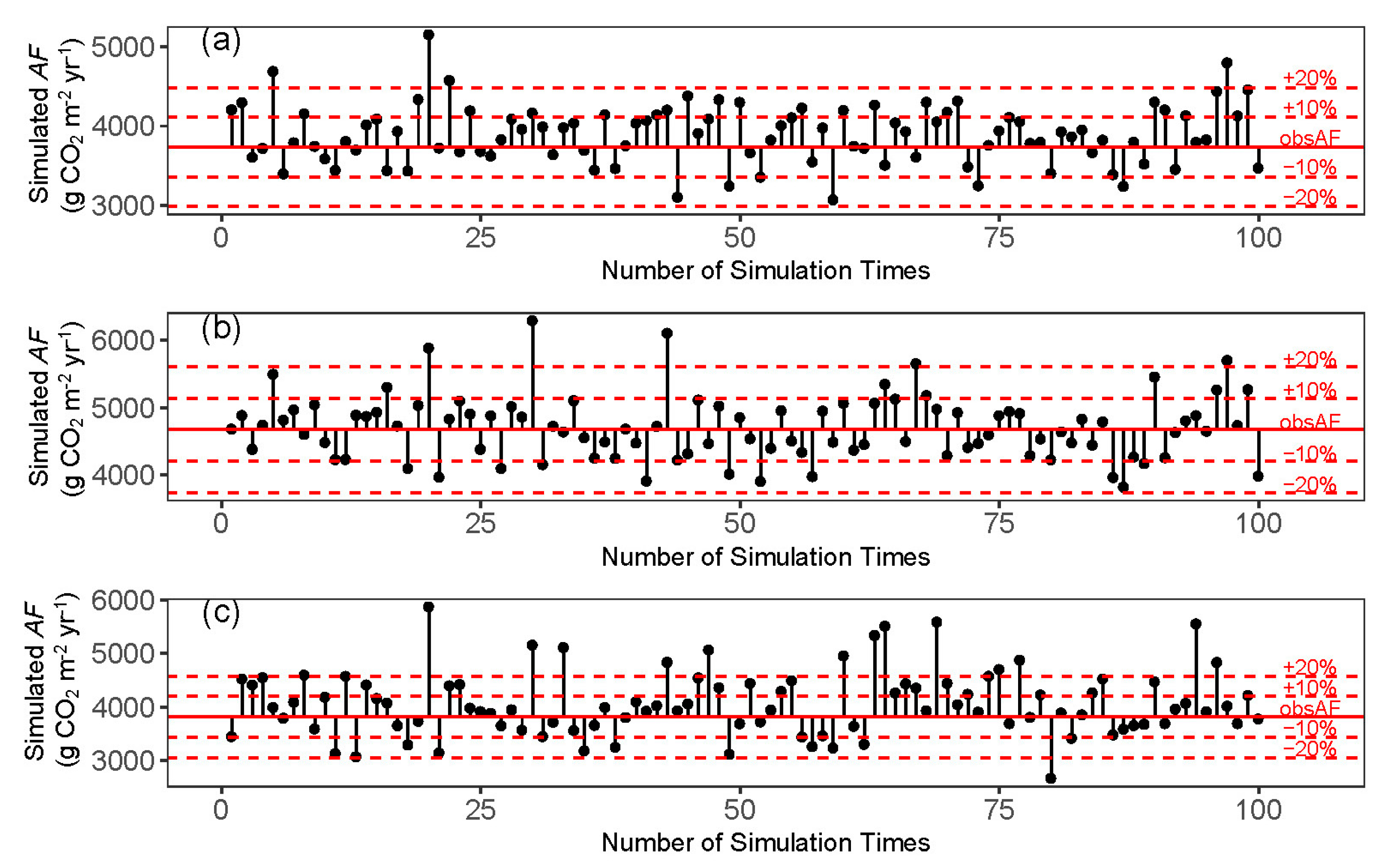
3.6. Testing Simulation Equation Using Eddy Covariance Data

For the 100 times simulation and verification of RECO, the R2 was 0.80–0.97, while the RMSE was 279–978 g CO2 m−2 yr1 (Figure 8). The R2 values of 94 out of 100 tests were higher than 0.85, while the RMSE values of 72 out of 100 tests was lower than 600 g CO2 m−2 yr−1. It is worth noting that higher RMSE values of RECO than that of soil respiration may be because RECO (ecosystem respiration) is generally larger than soil respiration (in the present study, the average value (mean ± standard deviation) was 2367 ± 1443 and 1014 ± 1441 g CO2 m−2 yr−1, respectively).

4. Discussion

4.1. Feasibility of Estimating AF Using Low-Frequency Flux Data Observations

The chamber method is an important means to observe the CO2 and CH4 fluxes of ecosystems. For global terrestrial ecosystems, flux observations using the chamber method have been carried out on at least 5000 plots [38], considerably more than for the eddy covariance method [39]. However, one disadvantage of the flux data obtained by the chamber method when operated manually is the low frequency of the data [40]. In addition, the sampling season and frequency of different observations are not standardized, making it difficult to compare the data, especially when large amounts of data are required for a comprehensive analysis at regional or global scales. Therefore, in the present study, we analyzed the relationship between the chamber-observed soil/ecosystem respiration and CH4 fluxes of different ‘candidate’ months and the total annual flux, AF. We developed and verified the AF estimation equations, and determined the feasibility of using low-frequency flux data for estimating the AF.
The results indicated a good linear fit between the soil/ecosystem respiration and CH4 fluxes of different months and the annual totals AFCO2 and AFCH4, respectively (Figure 2 and Figure 3). The equations also demonstrated good simulation ability. When only one month of flux was used to estimate the AFCO2 and AFCH4, the variability was explained by up to 67% and 92%, respectively. When the sampling frequency was increased to 4 months per year, this increased to 97% and 99%, respectively, while the RMSE corresponded to 292 g CO2 m−2 yr−1 and 4.0 g CH4 m−2 yr−1, respectively. This simulation performance is better than that found in previous studies. For example, 11 soil respiration model studies at national, regional, and global scales (presenting predictable proportions of 26–68%) were reviewed by Chen et al. [41], and previous work has been conducted on soil respiration simulation in China (RMSE = 799 g CO2 m−2 yr−1 [42]) and on global soil respiration [3,43,44]. The simulation error of soil CH4 fluxes using the present method also demonstrates a better simulation accuracy, yet it has rarely been discussed on an annual scale (RMSE = 76 g CH4 m−2 yr−1 [45]).
The efficacy of using a few monthly fluxes to determine the annual balance depends on the degree of seasonality of the flux. However, quite good performance was observed even when there was no distinct seasonality (Figure 9 and Figure 10). From the perspective of the processes and mechanisms of CO2 and CH4 emission/absorption, the observed flux itself is the result of the interaction of all environmental factors. Even one monthly flux provides a reliable reference for the emission/absorption magnitude of the observed environment when the flux is taken from a period with active biogeochemical reactions, for instance, in the summer or the growing season [46,47,48]. An increase in the number of monthly fluxes that were included in AF simulation, resulted in the better definition of the fluctuating extent in a year, thus increasing the exactness of the estimation. This was suspected to be a reason for the relatively good simulation accuracy when there was no distinct seasonality. Moreover, this also provided a possible explanation for why the simulation performance did not dramatically change across the different types of ecosystems or interfaces.
The high consistency between the estimated value and the observed value indicated a high feasibility of the method and equations for determining the AF. This implies that low-frequency flux data can be used to estimate the annual soil/ecosystem respiration and CH4 flux. Therefore, the great amount of archived sporadic chamber data can be brought together to contribute to future research on, for example, the process understanding of the carbon cycle, the cross-validation of multi-source flux data, and regional flux mapping, among others.

4.2. Selection of Sampling Months

Due to technical and budgetary constraints, soil greenhouse gas flux investigations are dominated by non-continuous low-frequency sampling. The question of when to sample has been plaguing researchers. This issue reflects the trade-off between input of budget and labor and spatiotemporal representativeness of the data. Although studies on soil greenhouse gas fluxes have been carried out for nearly 100 years, this question remains unanswered.
In the present study, we analyzed the impact of different months and different sampling frequencies on AF estimations. We found that, in general, the smaller the sampling frequency, the greater the discrepancy between different months (Figure 4), and the more important the timing. In addition, the summer or the warm season data were better suited for estimating the AF compared to the winter data. There is a much larger spatial flux difference in the warm season than in the winter [49,50,51]. Capturing the flux of a highly variable period was more effective in reducing the estimation error, which is presumed to be the reason why the warm period/growing season flux was more important for the AF estimation.
Based on our results, in the development of a monitoring plan for AF estimation, the number of observation months should be no less than four. The recommended months for soil/ecosystem respiration observations are May, July, September, and December (Equation (4)). The recommended months for the CH4 flux observation are January, June, July, and September (Equation (5)). When observing the soil/ecosystem respiration and CH4 fluxes together, the recommended months are March, May, August, and October (Equations (6) and (7)).
AFsimCO2 = 3.443 + 3.250 * MF5 + 1.805 * MF7 + 2.090 * MF9 + 4.270 * MF12,
AFsimCH4 = −0.043 + 3.266 * MF1 + 2.514 * MF6 + 0.994 * MF7 + 3.793 * MF9,
AFsimCO2 = 9.906 + 1.194 * MF3 + 3.710 * MF5 + 2.054 * MF8 + 3.117 * MF10,
AFsimCH4 = 0.858 + 3.694 * MF3 + 1.872 * MF5 + 0.904 * MF8 +9.514 * MF10,
In the present study, the optimal month/months were listed based on the statistical value but often, it can be difficult to carry out observations during the optimal sampling months. In this case, the sampling months can be selected using the R2 and RMSE values in the Tables S1–S4. For example, when using 4 monthly soil/ecosystem respirations and the AFII method to estimate the AFCO2, the months with similar estimation accuracies as the optimal selection (5, 7, 9, and 12) included 5, 7, 9, and 11 or 3, 5, 8, and 11 or 5, 8, 9 and 12 (Table S2).

4.3. Uncertainties

In the present study, we assumed that the flux data with a frequency of one or more times per month could represent the actual monthly flux. The annual flux was then derived by accumulating the monthly fluxes. However, the diurnal and seasonal variation [52,53,54,55] manifest obvious bias between the actual annual flux and the flux calculated based on infrequent observations. The flux difference between a low and high sampling frequency has been quantified at site scale. For instance, a study in a temperate rainforest carried out 1-year high-frequency (24 measurements per day) sampling of soil respiration [56], and randomly selected low-frequency data to calculate annual emission. This was compared to the full-data annual emission. The results revealed that when the annual sampling frequency was higher than once a month (the daily sampling frequency was once per day), the RMSE decreased to less than 10% of the annual emission. A similar bias was also reported by a continuous long-term study in a Korean monsoon forest [57]. Moreover, we did similar comparison using the eddy covariance data (Table 2) and found no significant difference (paired t-test: p > 0.05) among monthly ecosystem respirations (RECO) derived from continuous sampling and non-continuous sampling (simulated by generating partial-data series from full-data, Figure 11).
As the present AFobs is made up from the sum of the MF, it is obvious that there will (in general) be a correlation between the AFsim estimated from 1, 2, 3, 4 … months and the AFobs, and that the more MF being used, the higher the correlation will be. To identify if the correlation was just caused by the statistical method, we generated two sets of random data to represent random monthly soil/ecosystem respiration and CH4 fluxes. Considering data comparability, the data size and the range of values of the random datasets were consistent with the observed flux. The correlation analysis and the testing of the simulative equations were then repeated using the random datasets. Compared to the observed data, obviously weaker correlation (R values, Figure 2 and Figure 3, Table 4) and simulative performance (R2 and RMSE values, Figure 4) were observed using the random data. We suspect that the stronger correlation of the observed data was caused by seasonal patterns of flux. Thus, the statistic was speculated to be meaningful to understand the correlations between monthly and annual fluxes, although the correlations and simulative performance was very likely to be overestimated.
Considering that both the hypothesis and the statistical method introduced uncertainties into the simulation accuracy of the present equations, one critical question arises: Compared to the annual flux derived by high frequency measurement, how large is the error of the simulated annual flux that was calculated using the present method? Perez-Quezada et al. [56] published their full dataset of three automatic chambers. We therefore used their data to explore the question. One datum per required month of Equation (B4) (i.e., May, July, September and December) was randomly selected from the daytime observations (between 8 am and 6 pm, to keep the time consistent with the practice of the manual chamber technique). The simulated annual soil respiration was subsequently calculated using the equation and the selected data, and the data selection and simulation were repeated 300 times (100 times per chamber). Compared to the annual soil respiration determined from high frequency data (8592 observations per year, whose sum was denoted as obsAF in Figure 12), the simulated annual soil respiration (4 observations per year) showed a difference ranging from −30% to 54% of the obsAF (Figure 12), among which 276 simulated annual emissions exhibited a difference of −20% to 20% of the obsAF, while 193 simulated annual emissions exhibited a difference of −10% to 10%. Compared to Perez-Quezada’s [56] simulation of annual respiration (mean: 4288 g CO2 m−2 yr−1; RMSE: 538 g CO2 m−2 yr−1, 13% of the obsAF of 4150 g CO2 m−2 yr−1) using 4 day-time observations per year and their linear and non-linear models, the simulative accuracy of our simulation was slightly better (mean: 4212 g CO2 m−2 yr−1; RMSE: 507 g CO2 m−2 yr−1, 12% of the obsAF), which might benefit from month selection of the present study. Perez-Quezada’s study pointed out that no less than 2 observations per day (repeat 4 times per year) or no less than 1 observation per month is necessary to decrease RMSE to be lower than 10% of the obsAF. Inclusion of night-time observation can decrease RMSE to be lower than 5% of the obsAF with a sampling frequency of once per month. Using the Korean forest data [57], the estimated annual soil respiration using Equation (B4) was 7% lower than that calculated using the continuous data. Besides, the present method had also been tested using eddy covariance data. A good agreement (R2: 0.80–0.97; RMSE: 279–978 g CO2 m−2 yr−1) between simulated and observed ecosystem respiration (RECO) was observed (Figure 8). Although the simulative accuracy was good compared to previous studies, for example, studies on soil respiration simulation at global and ecosystem scales which showed RMSE values of 696–2010 g CO2 m−2 yr−1 [3,28,62,63]. It is worth note that the present RMSE values were still quite high (12–43% of the observed respiration), which calls for more efforts on ecosystem/soil respiration modeling.
The uncertainty analysis implies that although the equations above were developed using less-than-complete data, it did not nullify the present method, which we are proposing as a way to obtain annual flux. However, a deeper understanding of the estimation errors requires more continuous datasets and testing. In the future, when there is a sufficient continuous soil flux dataset, the simulation methods illustrated in the present study can be modified and improved.

5. Conclusions

In summary, the monthly fluxes largely varied with respect to the simulative performance of the annual flux. The summer or growing-season flux showed a higher simulative accuracy than winter. However, when the sampling could cover different seasons, a better simulation was observed than that of the clustered samples in the warm period. The presence of uncertainties in the present data and statistical method did not nullify the present method that we proposed to obtain the annual flux. The feasibility of the present method suggests that the large amount of archived sporadic chamber data can be combined to contribute to future research regarding the process of understanding the carbon cycle, cross-validation of multisource flux data, and regional flux mapping, among others. The comparison of the representativeness of different months can also be used to guide the selection of sampling months and to provide a reference for reducing workload and expenses for large-scale census or research projects with financial constraints.

Supplementary Materials

The following are available online at https://www.mdpi.com/2073-4433/10/10/623/s1, Table S1: Equations for annual soil/ecosystem respiration simulation and the predictive performance using method AFI, Table S2: Equations for annual soil/ecosystem respiration simulation and the predictive performance using method AFII, Table S3: Equations for annual CH4 flux simulation and the predictive performance using method AFI, Table S4: Equations for annual CH4 flux simulation and the predictive performance using method AFII.

Author Contributions

General idea design of the research: G.Y., N.H., Q.W., and M.Y., raw data collection: N.H., M.Y., Q.W. and Y.Z., data analysis: M.Y., and Y.Z., writing and editing: M.Y., J.G. and G.Y.

Funding

This research was funded by National Key Research and Development Program of China, grant number 2016YFA0600103; Chinese Academy of Sciences Strategic Priority Research Program, grant number XDA19020302; Young Scientists Fund, grant number 31800406; Major International (Regional) Joint Research Project, grant number 31420103917; Startup Program of Institute of Geographic Sciences and Natural Resources Research, Chinese Academy of Sciences, grant number Y6V60220YZ.

Acknowledgments

We thank Congcong Liu, Cuicui Jiao, Guangyan Song, Guili Zhu, Haili Yu, Hang Zhao, Jiahui Zhang, Jianxing Zhu, Jingjing Chang, Lang Han, Li Xu, Pu Yan, Qiongyu Zhang, Weikang Zhang, Ying Li, Yingqiu Cao, Yuan Liu and Yuqian Tang for their work on data extraction. We sincerely appreciate all anonymous reviewers who provide valuable suggestions and kind help on this paper.

Conflicts of Interest

The authors declare no conflict of interest. The funders had no role in the design of the study; in the collection, analyses, or interpretation of data; in the writing of the manuscript, or in the decision to publish the results.

References

  1. Ciais, P.; Sabine, C.; Bala, G.; Bopp, L.; Brovkin, V.; Canadell, J.; Chhabra, A.; DeFries, R.; Galloway, J.; Heimann, M.; et al. Carbon and other biogeochemical cycles. In Climate Change 2013: The Physical Science Basis: Contribution of Working Group I to the Fifth Assessment Report of the Intergovernmental Panel on Climate Change; Stocker, T.F., Qin, D., Plattner, G.K., Tignor, M., Allen, S.K., Boschung, J., Nauels, A., Xia, Y., Bex, V., Midgley, P.M., Eds.; Cambridge University Press: Cambridge, UK; New York, NY, USA, 2013; pp. 465–570. [Google Scholar]
  2. Lal, R. Soil carbon sequestration impacts on global climate change and food security. Science 2004, 304, 1623–1627. [Google Scholar] [CrossRef] [PubMed]
  3. Zhao, Z.; Peng, C.; Yang, Q.; Meng, F.; Song, X.; Chen, S.; Epule, T.E.; Li, P.; Zhu, Q. Model prediction of biome-specific global soil respiration from 1960 to 2012. Earth’s Future 2017, 5, 715–729. [Google Scholar] [CrossRef]
  4. Hashimoto, S.; Carvalhais, N.; Ito, A.; Migliavacca, M.; Nishina, K.; Reichstein, M. Global spatiotemporal distribution of soil respiration modeled using a global database. Biogeosciences 2015, 12, 4121–4132. [Google Scholar] [CrossRef] [Green Version]
  5. Myhre, G.; Shindell, D.; Bréon, F.M.; Collins, W.; Fuglestvedt, J.; Huang, J.; Koch, D.; Lamarque, J.F.; Lee, D.; Mendoza, B.; et al. Anthropogenic and Natural Radiative Forcing. In Climate change 2013: The physical Science Basis: Contribution of Working Group I to the Fifth Assessment Report of the Intergovernmental Panel on Climate Change; Stocker, T.F., Qin, D., Plattner, G.K., Tignor, M., Allen, S.K., Boschung, J., Nauels, A., Xia, Y., Bex, V., Midgley, P.M., Eds.; Cambridge University Press: Cambridge, UK; New York, NY, USA, 2013; pp. 659–740. [Google Scholar]
  6. Van den Pol-van Dasselaar, A.; van Beusichem, M.L.; Oenema, O. Effects of soil moisture content and temperature on methane uptake by grasslands on sandy soils. Plant Soil 1998, 204, 213–222. [Google Scholar] [CrossRef]
  7. Dlugokencky, E.J.; Nisbet, E.G.; Fisher, R.; Lowry, D. Global atmospheric methane: Budget, changes and dangers. Philos. Trans. R. Soc. A Math. Phys. Eng. Sci. 2011, 369, 2058–2072. [Google Scholar] [CrossRef] [PubMed]
  8. Bond-lamberty, B.; Thomson, A. A global database of soil respiration data. Biogeosciences 2010, 7, 1915–1926. [Google Scholar] [CrossRef] [Green Version]
  9. Oertel, C.; Matschullat, J.; Zurba, K.; Zimmermann, F.; Erasmi, S. Greenhouse gas emissions from soils—A review. Chem. Erde-Geochem. 2016, 76, 327–352. [Google Scholar] [CrossRef]
  10. Lundegardh, H. Carbon dioxide evolution of soil and crop growth. Soil Sci. 1927, 23, 417–453. [Google Scholar] [CrossRef]
  11. Savage, K.; Phillips, R.; Davidson, E. High temporal frequency measurements of greenhouse gas emissions from soils. Biogeosciences 2014, 11, 18277–18308. [Google Scholar] [CrossRef]
  12. Görres, C.M.; Kammann, C.; Ceulemans, R. Automation of soil flux chamber measurements: Potentials and pitfalls. Biogeosci. Disc. 2016, 13, 1949–1966. [Google Scholar] [CrossRef]
  13. Yao, Z.; Zheng, X.; Xie, B.; Liu, C.; Mei, B.; Dong, H.; Butterbach-Bahl, K.; Zhu, J. Comparison of manual and automated chambers for field measurements of N2O, CH4, CO2 fluxes from cultivated land. Atmos. Environ. 2009, 43, 1888–1896. [Google Scholar] [CrossRef]
  14. Lai, D.Y.F.; Roulet, N.T.; Humphreys, E.R.; Moore, T.R.; Dalva, M. The effect of atmospheric turbulence and chamber deployment period on autochamber CO2 and CH4 flux measurements in an ombrotrophic peatland. Biogeosciences 2012, 9, 3305–3322. [Google Scholar] [CrossRef]
  15. Hoffmann, M.; Wirth, S.J.; Beßler, H.; Engels, C.; Jochheim, H.; Sommer, M.; Augustin, J. Combining a root exclusion technique with continuous chamber and porous tube measurements for a pin-point separation of ecosystem respiration in croplands. J. Plant Nutr. Soil Sci. 2018, 181, 41–50. [Google Scholar] [CrossRef]
  16. Teramoto, M.; Liang, N.; Takagi, M.; Zeng, J.; Grace, J. Sustained acceleration of soil carbon decomposition observed in a 6-year warming experiment in a warm-temperate forest in southern Japan. Sci. Rep. 2016, 6, 35563. [Google Scholar] [CrossRef]
  17. Courtois, E.A.; Stahl, C.; Burban, B.; Van den Berge, J.; Berveiller, D.; Brechet, L.; Soong, J.L.; Arriga, N.; Penuelas, J.; Janssens, I.A. Automatic high-frequency measurements of full soil greenhouse gas fluxes in a tropical forest. Biogeosciences 2019, 16, 785–796. [Google Scholar] [CrossRef] [Green Version]
  18. Scholze, M.; Buchwitz, M.; Dorigo, W.; Guanter, L.; Shaun, Q. Reviews and syntheses: Systematic earth observations for use in terrestrial carbon cycle data assimilation systems. Biogeosciences 2017, 14, 3401–3429. [Google Scholar] [CrossRef]
  19. Papale, D.; Valentini, R. A new assessment of European forests carbon exchanges by eddy fluxes and artificial neural network spatialization. Glob. Chang. Biol. 2010, 9, 525–535. [Google Scholar] [CrossRef]
  20. Keenan, T.; Maria, S.J.; Lloret, F.; Ninyerola, M.; Sabate, S. Predicting the future of forests in the Mediterranean under climate change, with niche- and process-based models: CO2 matters. Glob. Chang. Biol. 2011, 17, 565–579. [Google Scholar] [CrossRef]
  21. Mcguire, A.D.; Sitch, S.; Clein, J.S.; Dargaville, R.; Esser, G.; Foley, J.; Heimann, M.; Joos, F.; Kaplan, J.; Kicklighter, D.W. Carbon balance of the terrestrial biosphere in the twentieth century: Analyses of CO2, climate and land use effects with four process—Based ecosystem models. Glob. Biogeochem. Cycles 2001, 15, 183–206. [Google Scholar] [CrossRef]
  22. Zhao, Y.; Ciais, P.; Peylin, P.; Viovy, N. How errors on meteorological variables impact simulated ecosystem fluxes: A case study for six French sites. Biogeosciences 2012, 9, 2537–2564. [Google Scholar] [CrossRef]
  23. Ruimy, A.; Saugier, B.; Dedieu, G. Methodology for the estimation of terrestrial net primary production from remotely sensed data. J. Geophys. Res. Atmos. 1994, 99, 5263–5283. [Google Scholar] [CrossRef]
  24. Estes, L.; Chen, P.; Debats, S.; Evans, T.; Ferreira, S.; Kuemmerle, T.; Ragazzo, G.; Sheffield, J.; Wolf, A.; Wood, E. A large-area, spatially continuous assessment of land cover map error and its impact on downstream analyses. Glob. Chang. Biol. 2017, 24, 322–337. [Google Scholar] [CrossRef] [PubMed]
  25. Demarty, M.; Bastien, J.; Tremblay, A. Carbon dioxide and methane annual emissions from two boreal reservoirs and nearby lakes in Quebec, Canada. Biogeosci. Discuss. 2009, 6, 2939–2963. [Google Scholar] [CrossRef] [Green Version]
  26. Liu, Y.; Yan, C.; Matthew, C.; Wood, B.; Hou, F. Key sources and seasonal dynamics of greenhouse gas fluxes from yak grazing systems on the Qinghai-Tibetan Plateau. Sci. Rep. 2017, 7, 40857. [Google Scholar] [CrossRef]
  27. Huang, Y. Study on carbon budget in terrestrial and marginal sea ecosystems of China. Bull. Chin. Acad. Sci. 2002, 17, 104–107. [Google Scholar]
  28. Jian, J.; Steele, M.K.; Thomas, R.Q.; Day, S.D.; Hodges, S.C. Constraining estimates of global soil respiration by quantifying sources of variability. Glob. Chang. Biol. 2018, 24, 4143–4159. [Google Scholar] [CrossRef]
  29. Xiao, J.; Zhuang, Q.; Law, B.E.; Baldocchi, D.D.; Chen, J.; Richardson, A.D.; Melillo, J.M.; Davis, K.J.; Hollinger, D.Y.; Wharton, S.; et al. Assessing net ecosystem carbon exchange of U.S. Terrestrial ecosystems by integrating eddy covariance flux measurements and satellite observations. Agric. Forest Meteorol. 2011, 151, 60–69. [Google Scholar] [CrossRef]
  30. FLUXNET2015 Dataset. Available online: https://fluxnet.fluxdata.org/data/fluxnet2015-dataset/ (accessed on 7 May 2018).
  31. R Core Team. R: A Language and Environment for Statistical Computing. R Foundation for Statistical Computing; R Core Team: Vienna, Austria, 2017; Available online: https://www.R-project.Org (accessed on 17 January 2019).
  32. Robinson, D.; Hayes, A. Broom: Convert Statistical Analysis Objects into Tidy Tibbles. R Package Version 0.5.1. 2018. Available online: https://cran.R-project.Org/package=broom (accessed on 17 January 2019).
  33. Wickham, H.; Francois, R.; Henry, L.; Müller, K. Dplyr: A Grammar of Data Manipulation. R Package Version 0.7.5. 2018. Available online: https://cran.R-project.Org/package=dplyr (accessed on 17 January 2019).
  34. Canty, A.; Ripley, B. Boot: Bootstrap r (s-plus) Functions. R Package Version 1.3-20. 2017. Available online: https://mirrors.tuna.tsinghua.edu.cn/CRAN/bin/windows/contrib/3.3/boot_1.3-20.zip (accessed on 17 January 2019).
  35. Peterson, B.G.; Carl, P. Performanceanalytics: Econometric Tools for Performance and Risk Analysis. R Package Version 1.5.2. 2018. Available online: https://mirrors.tuna.tsinghua.edu.cn/CRAN/bin/windows/contrib/3.4/PerformanceAnalytics_1.5.2.zip (accessed on 22 June 2019).
  36. Wickham, H. Ggplot2: Elegant Graphics for Data Analysis; Springer: New York, NY, USA, 2016. [Google Scholar]
  37. Kassambara, A. Ggpubr: ‘Ggplot2’ Based Publication Ready Plots. R Package Version 0.1.6. 2017. Available online: https://cran.R-project.Org/package=ggpubr (accessed on 17 January 2019).
  38. Bond-Lamberty, B.P.; Thomson, A.M. A Global Database of Soil Respiration Data, Version 4.1; ORNL Distributed Active Archive Center: Oak Ridge, TN, USA, 2018. [Google Scholar]
  39. Site Summary. Available online: https://fluxnet.fluxdata.org/sites/site-summary/ (accessed on 25 June 2019).
  40. Savage, K.E.; Davidson, E.A. A comparison of manual and automated systems for soil CO2 flux measurements: Trade-offs between spatial and temporal resolution. J. Exp. Bot. 2003, 54, 891–899. [Google Scholar] [CrossRef]
  41. Chen, S.; Zou, J.; Hu, Z. Measurements and modeling of soil respiration in terrestrial ecosystems. Ecol. Environ. Sci. 2017, 26, 1985–1996. [Google Scholar]
  42. Yu, G.; Zheng, Z.; Wang, Q.; Fu, Y.; Zhuang, J.; Sun, X.; Wang, Y. Spatiotemporal pattern of soil respiration of terrestrial ecosystems in China: The development of a geostatistical model and its simulation. Environ. Sci. Technol. 2010, 44, 6074–6080. [Google Scholar] [CrossRef]
  43. Chen, S.; Huang, Y.; Xie, W.; Zou, J.; Lu, Y.; Hu, Z. A new estimate of global soil respiration from 1970 to 2008. Chin. Sci. Bull. 2013, 58, 4153–4160. [Google Scholar] [CrossRef] [Green Version]
  44. Jian, J.; Steele, M.K.; Day, S.D.; Thomas, R.Q. Future global soil respiration rates will swell despite regional decreases in temperature sensitivity caused by rising temperature. Earth’s Future 2018, 6, 1539–1554. [Google Scholar] [CrossRef]
  45. Meng, L.; Hess, P.G.M.; Mahowald, N.M.; Yavitt, J.B.; Riley, W.J.; Subin, Z.M.; Lawrence, D.M.; Swenson, S.C.; Jauhiainen, J.; Fuka, D.R. Sensitivity of wetland methane emissions to model assumptions: Application and model testing against site observations. Biogeosciences 2011, 9, 2793–2819. [Google Scholar] [CrossRef]
  46. Lee, J.; McKnight, J.; Skinner, L.S.; Sherfy, A.; Tyler, D.; English, B. Soil carbon dioxide respiration in switchgrass fields: Assessing annual, seasonal and daily flux patterns. Soil Syst. 2018, 2, 13. [Google Scholar] [CrossRef]
  47. Lee, J.S. Monitoring soil respiration using an automatic operating chamber in a Gwangneung temperate deciduous forest. J. Ecol. Environ. 2011, 34, 411–423. [Google Scholar] [CrossRef]
  48. Morin, T.H.; Bohrer, G.; Stefanik, K.C.; Rey-Sanchez, A.C.; Matheny, A.M.; Mitsch, W.J. Combining eddy-covariance and chamber measurements to determine the methane budget from a small, heterogeneous urban floodplain wetland park. Agric. Forest Meteorol. 2017, 237, 160–170. [Google Scholar] [CrossRef]
  49. Zhang, G.B.; Ji, Y.; Ma, J.; Xu, H.; Cai, Z.C. Case study on effects of water management and rice straw incorporation in rice fields on production, oxidation, and emission of methane during fallow and following rice seasons. Soil Res. 2011, 49, 238–246. [Google Scholar] [CrossRef]
  50. Xu, X.; Riley, W.J.; Koven, C.D.; Billesbach, D.P.; Chang, R.Y.W.; Commane, R.; Euskirchen, E.S.; Hartery, S.; Harazono, Y.; Iwata, H. A multi-scale comparison of modeled and observed seasonal methane emissions in northern wetlands. Biogeosciences 2016, 13, 5043–5056. [Google Scholar] [CrossRef] [Green Version]
  51. Contosta, A.R.; Frey, S.D.; Cooper, A.B. Seasonal dynamics of soil respiration and N mineralization in chronically warmed and fertilized soils. Ecosphere 2011, 2, 1–21. [Google Scholar] [CrossRef]
  52. Sun, L.; Song, C.; Miao, Y.; Qiao, T.; Gong, C. Temporal and spatial variability of methane emissions in a northern temperate marsh. Atmos. Environ. 2013, 81, 356–363. [Google Scholar] [CrossRef]
  53. Liu, Y.; Han, S.J. Diurnal and seasonal variations in soil respiration in a temperate broad-leaved Korean pine forest, China. Appl. Mech. Mater. 2013, 295–298, 2318–2323. [Google Scholar] [CrossRef]
  54. Ma, L.; Zhong, M.; Zhu, Y.; Yang, H.; Johnson, D.A.; Rong, Y. Annual methane budgets of sheep grazing systems were regulated by grazing intensities in the temperate continental steppe: A two-year case study. Atmos. Environ. 2018, 174, 66–75. [Google Scholar] [CrossRef]
  55. Jammet, M.; Dengel, S.; Kettner, E.; Parmentier, F.J.W.; Wik, M.; Crill, P.; Friborg, T. Year-round CH4 and CO2 flux dynamics in two contrasting freshwater ecosystems of the subarctic. Biogeosciences 2017, 14, 5189–5216. [Google Scholar] [CrossRef]
  56. Perez-Quezada, J.F.; Brito, C.E.; Cabezas, J.; Galleguillos, M.; Fuentes, J.P.; Bown, H.E.; Franck, N. How many measurements are needed to estimate accurate daily and annual soil respiration fluxes? Analysis using data from a temperate rainforest. Biogeosciences 2016, 13, 6599–6609. [Google Scholar] [CrossRef] [Green Version]
  57. Eom, J.Y.; Jeong, S.H.; Chun, J.H.; Lee, J.H.; Lee, J.S. Long-term characteristics of soil respiration in a Korean cool-temperate deciduous forest in a monsoon climate. Anim. Cells Syst. 2018, 22, 100–108. [Google Scholar] [CrossRef]
  58. Guan, D.X.; Wu, J.B.; Zhao, X.S.; Han, S.J.; Yu, G.R.; Sun, X.M.; Jin, C.J. CO2 fluxes over an old, temperate mixed forest in northeastern China. Agric. Forest Meteorol. 2006, 137, 138–149. [Google Scholar] [CrossRef]
  59. Wang, M.; Li, Q.R.; Xiao, D.M.; Dong, B.L. Effects of soil temperature and soil water content on soil respiration in three forest types in changbai mountain. J. For. Res. 2004, 15, 113–118. [Google Scholar]
  60. Petersen, S.O.; Hoffmann, C.C.; Fer, C.M.S.; Blichermathiesen, G.; Elsgaard, L.; Kristensen, K.; Larsen, S.E.; Torp, S.B.; Greve, M.H. Annual emissions of CH4 and N2O, and ecosystem respiration, from eight organic soils in western Denmark managed by agriculture. Biogeosciences 2012, 9, 403–422. [Google Scholar] [CrossRef]
  61. Davidson, E.A.; Belk, E.; Boone, R.D. Soil water content and temperature as independent or confounded factors controlling soil respiration in a temperate mixed hardwood forest. Glob. Chang. Biol. 1998, 4, 217–227. [Google Scholar] [CrossRef] [Green Version]
  62. Chen, S.; Zou, J.; Hu, Z.; Chen, H.; Lu, Y. Global annual soil respiration in relation to climate, soil properties and vegetation characteristics: Summary of available data. Agric. Forest Meteorol. 2014, 198–199, 335–346. [Google Scholar] [CrossRef]
  63. Berryman, E.M.; Vanderhoof, M.K.; Bradford, J.B.; Hawbaker, T.J.; Henne, P.D.; Burns, S.P.; Frank, J.M.; Birdsey, R.A.; Ryan, M.G. Estimating soil respiration in a subalpine landscape using point, terrain, climate, and greenness data. J. Geophys. Res. Biogeosci. 2018, 123, 3231–3249. [Google Scholar] [CrossRef]
Figure 1. Location of the sampling sites of soil/ecosystem respiration and CH4 flux from different ecosystems.
Atmosphere 10 00623 g001
Figure 2. Correlation coefficient matrix of observed annual and monthly soil/ecosystem respiration. The diagonal panels represent the row and column heads, the numbers were the annual or monthly respiration (mean ± standard deviation, g CO2 m−2 yr−1 or g CO2 m−2 month−1). The numbers on x and y axis are respirations whose unit is g CO2 m−2 yr−1 for annual emission and g CO2 m−2 month−1 for monthly emission. The lower panels show the scatter plots (red lines are fitted lines of local regression) while the upper panels report the correlation coefficients. *** indicates significance at p < 0.001. The sample size is 330.
Atmosphere 10 00623 g002
Figure 3. Correlation coefficient matrix of observed annual and monthly CH4 fluxes. The diagonal panels represent the row and column heads, the numbers were the annual or monthly flux (mean ± standard deviation, g CH4 m−2 yr−1 or g CH4 m−2 month−1). The numbers on x and y axis are fluxes whose unit is g CH4 m−2 yr−1 for annual flux and g CH4 m−2 month−1 for monthly flux. The lower panels show the scatter plots (red lines are fitted lines of local regression) while the upper panels report the correlation coefficients. *** indicates significance at p < 0.001, ** indicates significance at p < 0.01, * indicates significance at p < 0.05. The sample size is 154.
Atmosphere 10 00623 g003
Figure 4. Maximum, minimum, and mean ± standard error of the R2 and RMSE values between AFobs and AFsim for simulations with different sampling frequencies. Results are based on 4094 linear regression equations for the arithmetic average (AFI) and weighted average (AFII) methods. The blue and red lines indicate the result of observed data of verification group (not used in equation development). The grey and black lines indicate the result of random data (for more information, see Section 4.3). The sample size is 106 for the soil/ecosystem respiration and 46 for the CH4 of both the observed data and the random data. All mean R2 and RMSE values are shown with the standard error, yet some are too small to be visible. Some symbols are overlapping, such that some symbols are invisible.
Atmosphere 10 00623 g004
Figure 5. RMSE values for simulations using fluxes from two months of the test data. (a) soil/ecosystem respiration; (b) CH4 flux.
Atmosphere 10 00623 g005
Figure 6. Comparison of the observed and estimated annual soil/ecosystem respiration using 1 to 4 monthly respirations of different types of ecosystem (ad) and interface (eh). Derived using Equations (B1)–(B4) in Table 3 and test data (not used in equation development). Respiration and RMSE unit: g CO2 m−2 yr−1.
Atmosphere 10 00623 g006
Figure 7. Comparison of the observed and estimated annual CH4 fluxes using 1 to 4 monthly fluxes of different types of ecosystem (ad) and interface (eh). Derived using Equations (B5)–(B8) in Table 3 and test data (not used in equation development). The small plots on the left are the enlarged portions of the small fluxes. Flux and RMSE unit: g CH4 m−2 yr−1. The sample size of water–air interface flux was only 2, therefore no regression line and RMSE values were presented.
Atmosphere 10 00623 g007
Figure 8. The distribution of R2 and RMSE values between observed and simulated ecosystem respiration (RECO) using eddy covariance data. (a) R2 between observed and simulated RECO. (b) RMSE between observed and simulated RECO.
Atmosphere 10 00623 g008
Figure 9. Agreement between simulated and observed annual soil/ecosystem respiration of data with or without a seasonal pattern. (a,b) are monthly variation of respiration with and without a seasonality, respectively. The respiration with one peak across a year was categorized as the with-seasonality group, whereas the respiration presenting several peaks or no obvious peak across a year was categorized as the without-seasonality group. (c,d) are simulation verification of respiration with or without seasonality, using one and four monthly respirations, respectively. The simulated respirations in (c,d) were derived using Equations (B1) and (B4) in Table 3, respectively.
Atmosphere 10 00623 g009
Figure 10. Agreement between simulated and observed annual CH4 flux of data with or without a seasonal pattern. (a,b) are monthly variation of flux with and without a seasonality, respectively. The flux with one peak across a year was categorized as the with-seasonality group, whereas the flux presenting several peaks or no obvious peak across a year was categorized as the without-seasonality. (c,d) are simulation verification of flux with or without seasonality, using one and four monthly fluxes, respectively. The simulated fluxes in (c,d) were derived using Equations (B5) and (B8) in Table 3, respectively. The small plots on the left of (c,d) are the enlarged portions of the small fluxes.
Atmosphere 10 00623 g010
Figure 11. Comparison of monthly ecosystem respirations among continuous (CS) and non-continuous sampling (NCS) using eddy covariance data. (a) Changling Grasslands; (b) Changbaishan Forest; see [58,59] for explanation on the high respiration; (c) Duolun Degraded Meadow; (d) Duolun Grassland; (e) Siziwang Grazed Grassland; (f) Haibei Permanent Wetland; (g) Haibei Grasslands; (h) Dangxiong Grassland; (i) Qianyanzhou Forest; (j) Dinghushan Forest. See Table 2 for more information. Data of NCS were generated by selecting observations from CS at different frequencies. CS are the eddy covariance timeseries and the NCS are the up-scaled calculated monthly sums using different half-hour emissions. CS: sum of all observations, i.e., 48 half-hour observations per day (48 observations per day * 30 days = 1440 observations per month). NCS1: calculated using 1 half-hour observation per day (1 observation per day * 30 days = 30 observations per month); as a common sampling time of manual chamber method [60,61], observation of 9:00–9:30 a.m. was selected as an example. NCS2: calculated using 10 half-hour observations per month, i.e., RECO of 9:00–9:30 a.m. on the 1st, 4th, 7th, 10th, 13th, 16th, 19th, 22nd, 25th and 28th. NCS3: calculated using 3 half-hour observations per month, i.e., RECO of 9:00–9:30 a.m. on the 5th, 15th, and 25th. NCS4: calculated using 1 half-hour observation per month, i.e., RECO of 9:00–9:30 a.m. on the 15th.
Atmosphere 10 00623 g011
Figure 12. Difference between continuous observed annual soil respiration and simulated annual soil respiration using the present method with four observations. (a) Chamber 1; (b) Chamber 2; (c) Chamber 3. The solid red horizontal line denotes the annual soil respiration using 8592 observations per year (obsAF); the black dots denote the simulated annual soil respiration using the 4 random observations per year required by Equation (B4), and simulation was carried out 100 times using each chamber data; the vertical black lines denote the difference between the simulated annual soil respiration and obsAF; the red dashed lines denote 4 references, and from top to bottom are 1.2, 1.1, 0.9, 0.8 times the obsAF, respectively. Raw data was obtained from Perez-Quezada et al. [56].
Atmosphere 10 00623 g012
Table 1. Basic information on the collected data.
ItemsSoil/Ecosystem RespirationCH4 Flux
Sample size (number of site-years)330154
Location19.4~47.6° N, 92.9~133.5° E19.4~47.6° N, 92.9~133.5° E
ChamberSelf-made or commercial transparent and opaque chamberSelf-made or commercial transparent and opaque chamber
Monitoring interface/sample sizeWater/8, soil/255, soil with no roots/25, soil and plants/42Water/9, soil/107, soil and plants/38
Ecosystem/sample sizeGrassland/26, forest/188, farmland/96, wetland/20Grassland/8, forest/66, farmland/56, wetland/24
Treatments or disturbancesFertilization, straw incorporation, cover crop, rotation, rotational grazing, grazing, rain protection, root cutting, fire, herbicide application, harvesting, reclamation, increase and decrease of litterFertilization, straw incorporation, covering, crop rotation, rotational grazing, grazing, rain reduction,
Fluxes range14.0~7514.0 g CO2 m−2 yr−1 *−21.0~377.6 g CH4 m−2 yr−1
Mean ± standard deviation of fluxes1014 ± 1441 g CO2 m−2 yr−113.8 ± 49.8 g CH4 m−2 yr−1
Median of fluxes321 g CO2 m−2 yr−1−0.16 g CH4 m−2 yr−1
Note: * Positive values indicate CO2 loss. There is no CO2 gain because all the observations with plant used opaque chamber (no photosynthesis).
Table 2. Basic information on the 10 flux observation sites using eddy covariance technique. Mean ± standard deviation of fluxes of all site-years: 2367 ± 1443 g CO2 m−2 yr−1, median of fluxes of all site-years: 1932 g CO2 m−2 yr−1. Data of the site Siziwang in 2010 and 2012 is several magnitudes lower than in 2011 and other sites with no explanation, therefore, data of these two years were excluded.
Site NameEcosystemLatitudeLongitudeDurationMean ± Standard Deviation of Fluxes (g CO2 m−2 yr−1)Median of Flux (g CO2 m−2 yr−1)
ChanglingGrasslands44.6 123.5 2007–20101382 ± 1351384
ChangbaishanMixed Forests42.4 128.1 2003–20054459 ± 4324608
Duolun Degraded MeadowGrasslands42.1116.32009–20101425 ± 91425
Duolun GrasslandGrasslands42.0116.32007–2008881 ± 385881
Siziwang GrazedGrasslands41.8111.92011798798
Haibei ShrublandPermanent Wetlands37.6 101.3 2003–20052488 ± 1782406
Haibei Alpine TibetGrasslands37.4 101.2 2002–20041437 ± 8581879
DangxiongGrasslands30.5 91.1 2004–2005809 ± 25809
QianyanzhouEvergreen Needleleaf Forests26.7 115.1 2003–20054402 ± 3074282
DinghushanEvergreen Broadleaf Forests23.2 112.5 2003–20053545 ± 973588
Table 3. The best (RMSE minimum) and worst (RMSE maximum) AFCO2 and AFCH4 estimating equations using data from 1 to 4 months. Remaining equations are shown in Tables S2 and S4. To provide more information on equations performance, the corresponding R2 and RMSE values of training data are also reported. AFsim (g m−2 yr−1) is the simulated annual cumulative flux; MFn (g m−2 month−1) indicates the observed monthly flux of different months, for example, MF7 represents the monthly flux of July and MF5 represents the monthly flux of May.
GasModelNumber of Months Included in the ModelEquation No.The Best ModelTraining DataTest DataEquation No.The Worst ModelTraining DataTest Data
R2RMSER2RMSER2RMSER2RMSE
CO2Model AFII 1B1AFsimCO2 = 71.901 + 5.021 * MF7 0.651910.6651186W1AFsimCO2 = 137.159 + 15.082 * MF1 0.5281060.3491968
2B2AFsimCO2 = 22.282 + 5.086 * MF5 + 3.614 * MF90.902480.889584W2AFsimCO2 = 132.480 + 9.691 * MF1 + 5.063 * MF20.5611020.4241789
3B3AFsimCO2 = 19.844 + 4.301 * MF5 + 2.993 * MF9 + 3.999 * MF120.928410.941431W3AFsimCO2 = 122.230 + 9.430 * MF1 + 2.506* MF2 + 2.885* MF30.5791000.4491683
4B4AFsimCO2 = 3.443 + 3.250 * MF5 + 1.805 * MF7 + 2.090 * MF9 + 4.270 * MF120.971260.969292W4AFsimCO2 = 93.022 + 7.112 * MF1 + 1.660 * MF2 − 0.574 * MF3 + 5.188* MF40.692850.5971306
CH4Model AFII1B5AFsimCH4 = 3.868 + 19.192 * MF100.87018.50.91514.8W5AFsimCH4 = 7.477 − 25.990 * MF11 0.62631.30.90678.5
2B6AFsimCH4 = −1.181 + 2.682 * MF4 + 4.530 * MF7 0.9728.50.9885.2W6AFsimCH4 = 5.033 + 9.092 * MF2 − 24.388 * MF11 0.68928.60.89369.6
3B7AFsimCH4 = −1.321 + 1.545 * MF1 + 2.582 * MF4 + 4.463 * MF70.9738.40.9885.0W7AFsimCH4 = 2.370 − 5.427 * MF2 + 15.394 * MF3 − 18.675 * MF110.81322.10.79262.0
4B8AFsimCH4 = −0.043 + 3.266 * MF1 + 2.514 * MF6 + 0.994 * MF7 + 3.793 * MF90.9856.20.9934.0W8AFsimCH4 = 2.093 + 3.361 * MF1 − 5.378 * MF2 + 14.480 * MF3 − 17.307 * MF110.81721.90.63659.5
Table 4. Correlation coefficient R between each group and the sum of the random datasets. Groups 1–12 represent random monthly flux while the sum represents the random annual flux.
GroupsRandom Dataset 1Random Dataset 2
Rp ValueSample SizeRp ValueSample Size
Group 10.21<0.0013300.27<0.01154
Group 20.34<0.0013300.28<0.001154
Group 30.28<0.0013300.32<0.001154
Group 40.31<0.0013300.33<0.001154
Group 50.35<0.0013300.15>0.05154
Group 60.34<0.0013300.38<0.001154
Group 70.25<0.0013300.19<0.05154
Group 80.30<0.0013300.37<0.001154
Group 90.24<0.0013300.20<0.05154
Group 100.29<0.0013300.41<0.001154
Group 110.34<0.0013300.16<0.05154
Group 120.31<0.0013300.29<0.001154

