Aerosol Particle and Black Carbon Emission Factors of Vehicular Fleet in Manila, Philippines

Abstract

Poor air quality has been identified as one of the main risks to human health, especially in developing regions, where the information on physical chemical properties of air pollutants is lacking. To bridge this gap, we conducted an intensive measurement campaign in Manila, Philippines to determine the emission factors (EFs) of particle number (PN) and equivalent black carbon (BC). The focus was on public utility jeepneys (PUJ), equipped with old technology diesel engines, widely used for public transportation. The EFs were determined by aerosol physical measurements, fleet information, and modeled dilution using the Operational Street Pollution Model (OSPM). The results show that average vehicle EFs of PN and BC in Manila is up to two orders of magnitude higher than European emission standards. Furthermore, a PUJ emits up to seven times more than a light-duty vehicles (LDVs) and contribute to more than 60% of BC emission in Manila. Unfortunately, traffic restrictions for heavy-duty vehicles do not apply to PUJs. The results presented in this work provide a framework to help support targeted traffic interventions to improve urban air quality not only in Manila, but also in other countries with a similar fleet composed of old-technology vehicles.

1. Introduction

Degradation of air quality, especially in developing regions, was shown to be related to road traffic [1]. The particulate emissions from traffic are mainly linked to elevated number concentrations of ultrafine particles (UFPs, diameter less than 100 nm). UFPs can deeply penetrate into the lungs [2] and cause negative health responses [3]. Moreover, combustion related particles, black carbon (BC) or soot, often contain toxic trace compounds [4,5], which were shown to negatively impact human health [6].

The problem of traffic-related particulate pollution was recognized in higher income countries and addressed by improving vehicle engine technology and fuel quality [5,7]. Introduction of diesel particle filters [8] and implementation of low emission zones [9] demonstrated to be useful methods to improve urban air quality [10]. Such strategies, on the other hand, are rarely practiced in the developing regions, due to economic and behavioral factors. Here, significant portions of pre-Euro-standard vehicles still remain in use for public transportation [11]. Previously mentioned strategies to control vehicle emissions are often too expensive and not seen as practical to be implemented into old-technology vehicles. The severity of the problem is amplified by insufficient monitoring of the core pollutants, e.g., black carbon (BC), due to lack of instrumentation and expertise. Consequently, a detailed inventory of urban road traffic emissions is yet to be generated, which in turn will allow modeling of air quality and to develop strategies for mitigation of particulate traffic emissions.

Emission factors (EF), a parameter describing the concentration of pollutant emitted within a driven distance (or amount of fuel burnt) [12], serve as an input in many urban air quality models [13]. Numerous laboratory-based and real-world studies of aerosol EF were conducted in Europe, US, Australia, China, and India [14,15,16,17,18,19]. From the literature study, it is evident that the majority of EF studies were conducted in mid- to highly developed countries. On the other hand, in regions where road traffic-related pollution is the highest, EF studies are often left behind due to technical difficulties and incapacities.

The main objectives of this study are: (1) to address the concern of air pollution issue in a developing region of Southeast Asia by providing an inventory of the road-traffic related particle number (PN) and equivalent black carbon (BC) emission factors for the average vehicle, public utility jeepneys (PUJs), and light-duty vehicles (LDVs); (2) as well as to raise the awareness about air quality in developing regions, where the pollution is dominated by traffic-related emissions of incomplete combustion. Metro Manila, the capital of the Philippines, was chosen as the domain for this study. It is one of the most densely populated cities in the world (information available at https://population.un.org/wup/Maps/ (Accessed 30 June 2019)). Here, the most commonly used public transportation is based on PUJs, vehicles equipped with old-technology diesel. Emissions from PUJs have recently been identified as the major contributor to elevated emissions of BC in Metro Manila [20].

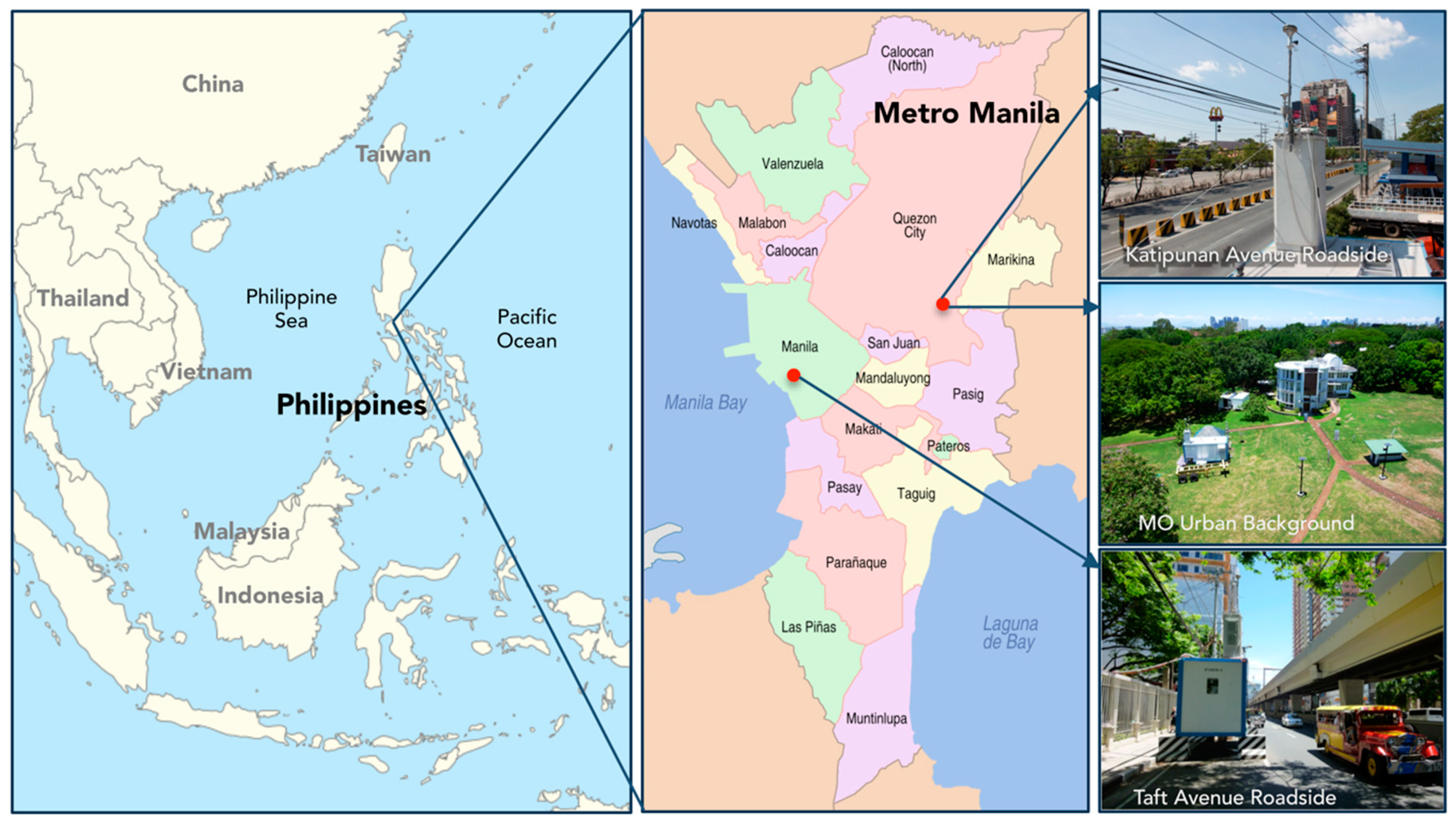
2. Measurement Set-Up

The particle number size distribution (size range from 10 nm to 10 μm), equivalent black carbon (BC) mass concentration, meteorological conditions, and traffic information were collected during an intensive measurement campaign called Manila Aerosol Characterization Experiment in 2015 (MACE 2015). The campaign was designed to investigate the properties of road-traffic related particulate pollution in a highly urbanized area of Metro Manila. The MACE 2015 campaign was organized by the Leibniz-Institute for Tropospheric Research (TROPOS) and the consortium “Researchers for Clean Air” (RESCueAir) in three stages from March to June, 2015. The first stage of the campaign consisted of sampling days between 1 April–5 May at Katipunan Avenue (roadside site), followed by an inter-comparison stage located at the Manila Observatory (urban background site) from 7–14 May, and last stage was at Taft Avenue (roadside site) during 18 May–10 June (Figure 1). The data used in this work is during the last stage of the campaign when the measurement container was placed in a street canyon. A detailed description of the campaign stages can be found in Alas et al. [21] and Kecorius et al. [20].

2.1. Street Configuration at Taft Avenue

Taft Avenue (14.56° N, 120.99° E) is composed of six lanes, three lanes each direction. The measurement container was placed in one of the southbound lanes (Figure 2, left). A traffic light was about 100 m south from the measurement container. A distinctive feature of the area was the elevated light-rail train track in the middle of the road (7 m above the street). The street width is 30 m, and the average canyon height is 60 m. This type of street (street aspect ratio (H/W) of 2.0) corresponds to a deep street canyon [22]. The corresponding sketch (see Figure 2, right) represents the street configuration used in the modeling of the dilution factor. Taft Ave. is often congested due to the surrounding commercial establishments. A stop-and-go driving behavior was frequently observed during the daytime. During nighttime, the traffic flow was more steady with vehicle speeds no more than 50 km h⁻¹.

2.2. Instrumentation

The aerosol sampling line on top of the mobile measurement container consisted of a PM₁₀ inlet (16.67 L min⁻¹, approx. 5 m a.s.l), two 1.5-meter long Nafion driers (15 mm inner diameter), and an automatic drying chamber [23]. Inside the container, the aerosol flow was divided between the instruments using an isokinetic splitter and conductive stainless steel tubing. A TROPOS-type Mobility Particle Size Spectrometer (MPSS) [24] was used to measure the particle number size distribution (PNSD) in the size range from 10–800 nm (mobility diameter) with a time resolution of 2.5 min. The system uses a Hauke-type Differential Mobility Analyzer (DMA) and Condensation Particle Counter (CPC, model 3772, TSI Inc., Shoreview, MN, USA, flow rate 1 L min⁻¹). The larger particles in the size range from 500 nm–10 µm (aerodynamic diameter) were measured using an Aerodynamic Particle Size Spectrometer (APS, model 3221, TSI Inc., USA). Nebulized polystyrene latex spheres (203, 1000, and 2000 nm, Thermo Scientific™, Waltham, MA, USA, Duke Standards™) were used to ensure the sizing accuracy of both MPSS and APSS as suggested in Wiedensohler et al. [25] and Pfeifer et al. [26]. Other data quality routines included, e.g., regular zero checks (detecting leaks in the plumbing lines), and high voltage calibration (for MPSS) that were done on a regular basis (once per week).

To obtain particle number size distribution from 10 nm to 10 µm (volume equivalent diameter), PNSDs from MPSS and APS were merged using an enhanced inversion algorithm [27]. We used a density of 1.8 g cm⁻³, which corresponds to diesel soot particles [28]. The dynamic shape factor profile was retrieved from the best fit of overlapping MPSS and APS PNSDs and ranged from 1.5 to 2.5, which is in good agreement with the previous study on soot particle shape factor [29]. The merged PNSDs were used to calculate particle surface area, volume and mass concentrations in different size ranges (see Supplementary Material Table S1). Note that in the literature, different size ranges were presented for PN EFs (e.g., Wang et al. [15]). In this work, we chose the size intervals as in Birmili et al. [30] for comparison purposes.

The equivalent black carbon (BC) mass concentration was measured using a Multi-Angle Absorption Photometer (MAAP Model 5012, Thermo, Inc., Waltham, MA USA) [31]. The MAAP flow was adjusted to 3 L min⁻¹ to save the fiber filter in the heavily polluted environment. Meteorological parameters, such as wind speed and direction, ambient temperature, relative humidity (RH), global radiation, and precipitation was measured using automatic weather stations both at the rooftop of the measurement container and a De La Salle University building and can be found in the supplementary material (Table S2, Figure S1). Briefly, the measurement campaign took place during both dry and wet seasons [20]. In this study, we have excluded time periods with occasional rain events, which could influence the measurement results. The average temperature, wind speed and relative humidity (RH) in Taft Ave. during measurement period was 31 ± 2 °C, 0.8 ± 0.4 m s⁻¹, 69 ± 8%, respectively. The prevailing wind direction during the daytime was southwest and northwest, which is almost perpendicular and parallel to Taft Avenue, respectively.

2.3. Estimation of Emission Factors (EF)

In this work, an inverse modeling approach was used to determine the road traffic EFs of aerosol particle number and equivalent black carbon [12]. The EF_i,k of the pollutant i and kth vehicle category can be calculated from the equation:

$$E{F}_{i,k}\left[\frac{1 }{km·veh}\right]=(\frac{\Delta C_i }{F})/{{\displaystyle \sum }}_k{N}_k\left[\frac{veh}{s}\right],$$

(1)

where $\Delta C_i$ is the difference between curbside and background pollutant concentration, F (s m⁻²) is the dilution factor modeled using the OSPM, and N_k is the traffic flow of kth vehicle category. Because the total emission along the curbside can be seen as the superposition of each vehicle group category, we can separate the emission of the fleet into LDVs and jeepneys (PUJs), rewriting Equation (1) as:

$$E{F}_{Total}=E{F}_{i, LDVs}·\frac{N_{LDV} }{N_{Total}}+E{F}_{i, PUJs}·\frac{N_{PUJ} }{N_{Total}}+ {\epsilon }_i,$$

(2)

where $E{F}_{i, LDV}$ and $E{F}_{i,Jeepney}$ are the emission factor of the pollutant i, $\frac{N_{LDV}}{N_{Total}}$and $\frac{N_{PUJ}}{N_{Total}}$ are the number fraction of LDVs and PUJs, and ${\epsilon }_i$ is the residual component. Equation (2) is solved by bivariate linear regression resulting in a plane where the slope represents the EF of the kth vehicle category and the uncertainty of the slope is an estimate of the uncertainties of the EF originating from the concentration measurements and the F [32].

2.3.1. Determination of Curbside Contribution

Road traffic contribution to measured pollutant concentration can be calculated as the difference between the curbside (C_curbside) and background (C_background) pollution concentrations:

$$\Delta C \left(t\right)=C_{curbside}\left(t\right)-C_{background}\left(t\right).$$

(3)

The curbside concentration is a superposition of the (1) urban background concentration that is the result of both regional and continental concentrations, and the (2) direct tailpipe emissions of the vehicles in that street. Kakosimos et al. [33] presents several methods to estimate $\Delta C$. The urban background pollutant concentrations can be obtained from a nearby measurement station that is not affected by direct emissions. If urban background measurements are not available, nighttime curbside pollutant concentration can be used [34]. In this study, we determined the background PN and BC mass concentrations by applying the rolling minimum method [20]. The method was shown to accurately estimate (uncertainty of <5%) the background concentration at the curbside when urban background measurements are lacking. We prefer this method over constant nighttime values, because it was shown that background concentration in urban environment is not constant. The retrieved urban background concentrations and the results of the bivariate linear regression can be found in Supplementary Material Figures S2 and S3, respectively.

2.3.2. Dilution and Emission Factors

The OSPM model was used to obtain the dilution factor (F), used in EF calculation as:

$$F=\left(\sqrt{\frac{2}{\pi }}\right)\frac{1}{W\sqrt{{\left(a{u}_b\right)}^2+{\sigma }_t^2}}ln\left(1+\frac{\sqrt{{\left(a{u}_b\right)}^2+{\sigma }_t^2}{L}_r}{u_b{h}_0}\right)+\frac{L_r}{W\left({\sigma }_{wt}{L}_t+u_d{L}_S\right)},$$

(4)

where W is the street width, u_b is the wind speed at the street level, u_d the speed of convection, h₀ the initial dispersion parameter, a an empirical constant (0.1), ${\sigma }_t$ the traffic-induced turbulence, θ the angle of wind direction and street axis, ${\sigma }_{wt}$is the flux velocity, L_r,t,s is the length, top edge, and side edge of the recirculation zone, respectively. In brief, the factor F in OSPM is based on the combination of a plume model for the emissions that are directly transported from the vehicle exhaust to the sampling inlet of the monitoring station and a box model for the emission that recirculates in the street canyon by a vortex flow. A more detailed discussion of the model is provided by Berkowicz et al. [12] and Xia [35], and it is briefly illustrated in Supplementary Material (Figure S4).

3. Results and Discussion

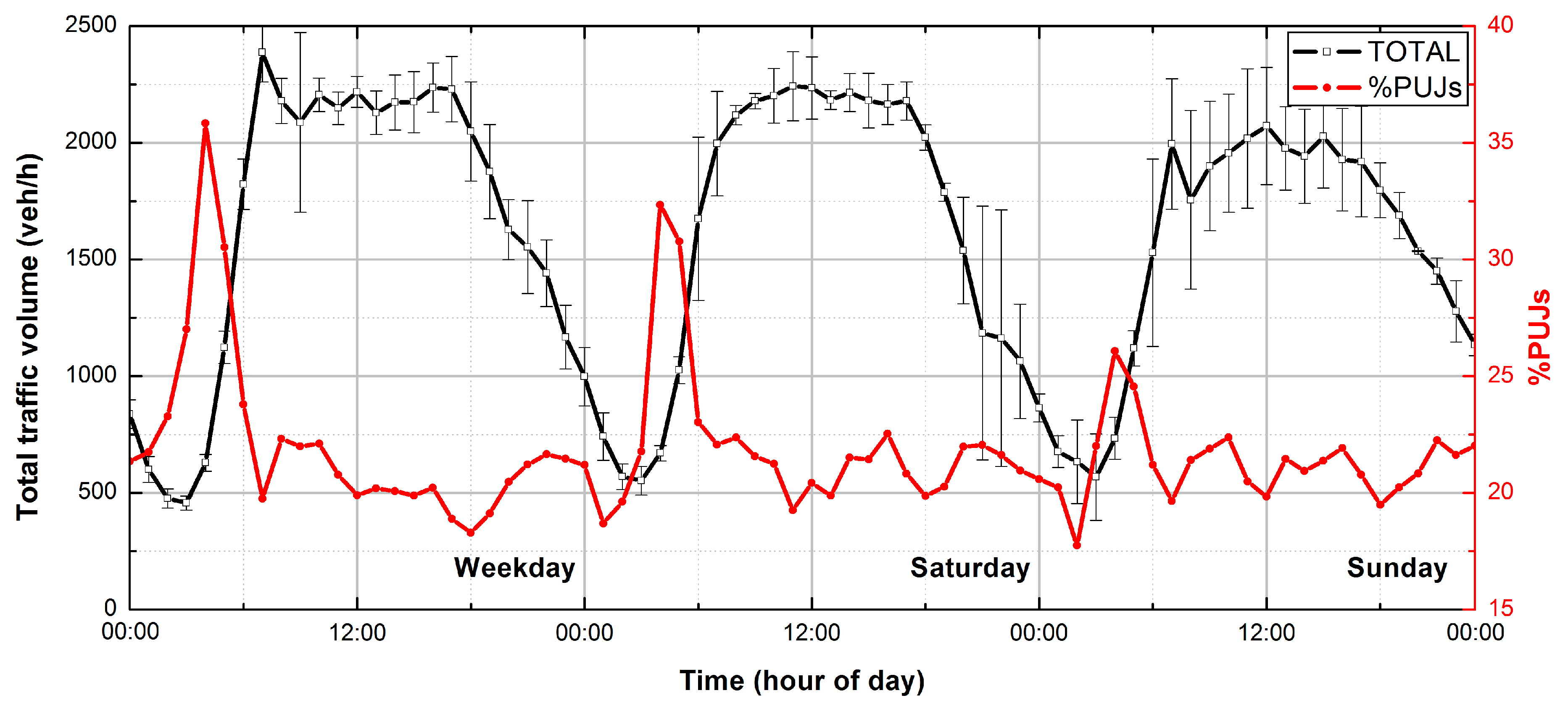
3.1. Traffic Conditions

Traffic flow in street canyon was characterized by manually counting the passing vehicles from continuous street videos. The traffic fleet was divided into two classes: (a) the light-duty vehicle (LDVs), which consists of passenger cars, motorbikes, tricycles; and (b) heavy-duty vehicles, including buses, delivery trucks, and jeepneys (PUJs). Please note that the traffic was counted for one direction flow only. The total vehicle number was obtained by multiplying the vehicle count by two. Possibly introduced uncertainties are discussed in Section 4. Due to a scheduled traffic regulation at Taft Ave., most delivery trucks and buses are not allowed to traverse the avenue. Thus, the heavy-duty vehicle category is dominated by PUJs (up to 94%). The average daily traffic density during the measurement campaign was 40,000 ± 120 vehicles per day. The average diurnal variation of the total traffic volume and the fraction of PUJ are shown in Figure 3.

During all the days of the week, the traffic volume on the street between 06:00 and 18:00 were rather stable with more than 2000 vehicles h⁻¹. A slight increase can be noticed during morning (06:00 to 09:00), lunch (11:00 to 13:00), and afternoon (16:00 to 18:00) rush hours. Traffic volume subsides from around 18:00 and reaches its minimum of 500 vehicles h⁻¹ at approx. 03:00, after which it starts to increase again. On average, the PUJ share was 20% of the total traffic volume, but this share increases during nighttime, as it becomes the main means of public transportation along the avenue. A sample traffic video at Taft Ave. is provided by Kecorius et al. [20].

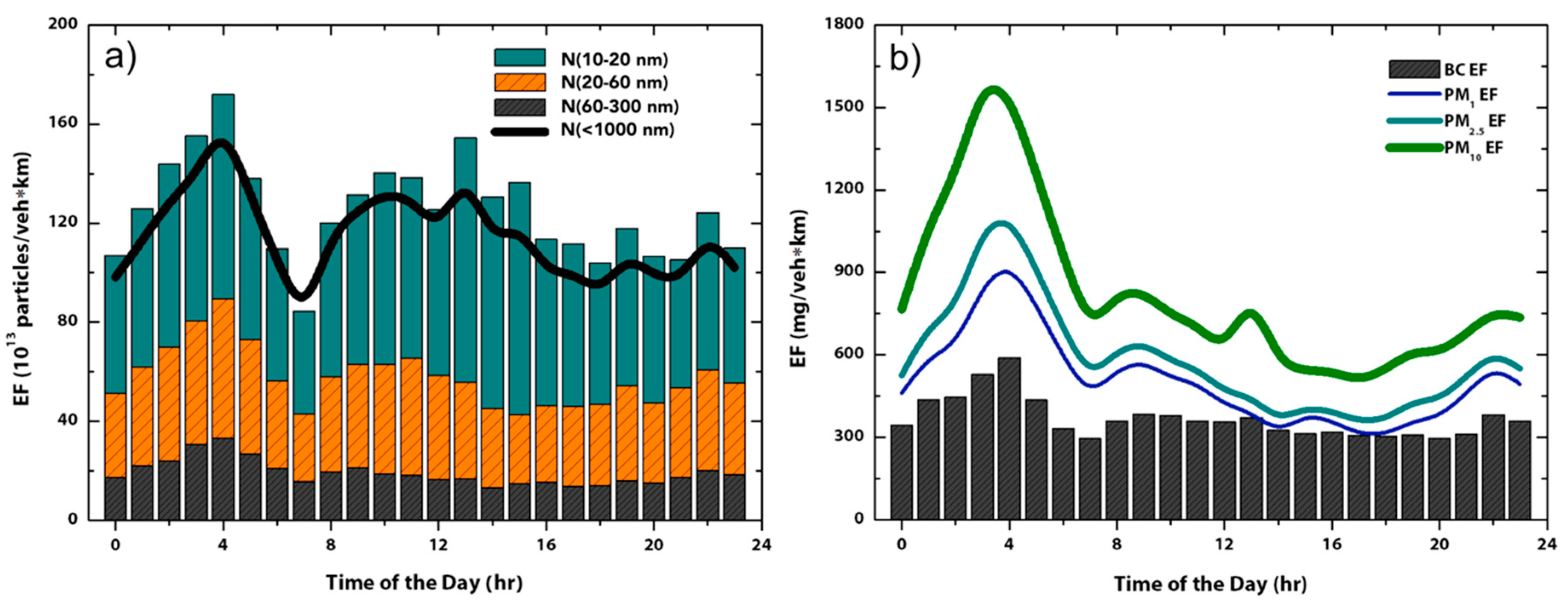
3.2. Mixed Fleet Emission Factor

The average diurnal variation of the size-segregated PN and the BC EFs for the mixed fleet at Taft Avenue is presented in Figure 4a,b, respectively. For reference, Figure 4b includes the PM₁, PM_2.5, and PM₁₀ mass EF (derived from merged PNSDs). Results are also summarized in

Table 1. Summary of particle number (PN) and BC mass emission factor (EF) compared to values from literature. Note that in case of Manila, column for heavy-duty vehicles (HDV) represents the EFs of public utility jeepneys (PUJs). Results for passenger-car like vehicles, which include light-duty vehicles (LDV), were compared with published emission factors of LDVs. We present results as mean EF (± standard error) and mean EF (± standard error or standard deviation) for other studies. YoM—year of measurements.

Study	YoM	Site		Fleet	LDV	HDV
			Mass Emission Factor (mg/veh·km)
This study	2015	Urban	BC	336 ± 4.2	179 ± 4.2	1260 ± 50
Zurich, Switzerland [38]	2002	Urban	BC	35 ± 3.0	10 ± 1.0	427 ± 33
São Paolo, Brazil [41]	2004	Tunnel	BC	-	16 ± 5	462 ± 112
Beijing, China [18]	2007	Urban	BC	-	26.6	1220
Manila, Philippines [20]	2015	Urban	BC	313	27	1620
Londrina, Brazil [42]	2016	Urban	BC	-	26 ± 12	691 ± 67
São Paolo, Brazil [43]	2015	Highway	BC	-	41 ± 63	170 ± 259
			Number Emission Factor (1013 particles/veh·km)
This study	2015	Urban	N10–20	53.5 ± 0.64	22.4 ± 4.3	137 ± 14
			N20–60	41.0 ± 0.43	24.2 ± 2.8	124 ± 9.7
			N60–300	17.6 ± 0.20	10.0 ± 1.3	65.9 ± 4.3
			N300–800	0.15 ± 0.003	0.09 ± 0.02	0.64 ± 0.06
			N<1000	106 ± 1.1	55.6 ± 7.0	330 ± 24
Copenhagen, Denmark [32]	2001	Urban	N10–700	28	-	-
Zurich, Switzerland [38]	2002	Urban	N18–50	6.4 ± 0.4	2.6 ± 0.2	73 ± 3
			N18–100	9.0 ± 0.5	3.8 ± 0.2	105 ± 3
			N18–300	11.2 ± 0.7	4.6 ± 0.2	132 ± 3
			N>7	38.6 ± 1.8	8.0 ± 0.9	550 ± 10
London, UK [44]	2003	Urban	N11–437	-	5.8	63.6
Berlin, Germany [45]	2005	Urban	N10–500	21 ± 2	2.4 ± 1.5	296 ± 35
Leipzig, Germany [8]	2006	Urban	N4–800	-	54 ± 2	4300 ± 1700
Copenhagen, Denmark [15]	2008	Urban	N10–50	10.1 ± 0.24	3.9 ± 0.48	155 ± 10
		Urban	N50–100	4.70 ± 0.14	3.4 ± 0.31	33.5 ± 6.4
		Urban	N100–700	2.02 ± 0.11	0.86 ± 0.24	29.0 ± 0.50
		Urban	N10–700	18.7 ± 3.0	10 ± 0.6	221 ± 13
		Highway	N10–700	21.5 ± 0.53	8.1 ± 0.69	175 ± 6.8
Londrina, Brazil [42]	2016	Urban	N<1000	-	92.5 ± 11	373 ± 58

, where comparisons with other studies are added. Readers are recommended to visit the Supplementary Material (Tables S3 and S4) for auxiliary information on particle surface area, particle volume, and particle mass EFs.

The first distinct feature that can be seen in Figure 4 is the oddly high value of EF for both particle number and mass EF during early morning hours (03:00 to 05:00). During this time, EF values are almost twice as large as the daily average. A similar increase in particulate EF during nighttime was also observed in other studies [5,8,32] and has no straightforward explanation. One possible reason for higher EFs could be the inaccuracy of vehicle counts collected during nighttime or darkness [36,37], as headlights from vehicle obstructs the manual counting from nighttime video footages. On the other hand, the odd increase of EF might be attributed to the prevalence of diesel vehicles during nighttime. This was observed in an EF study [32] in an urban street in Copenhagen, Denmark where diesel taxis dominate during nighttime. In their study, the authors speculated that the increased fraction of diesel-powered vehicles, which are known to generate higher emissions, caused the increase of EF during nighttime. In this study, EFs’ variability during nighttime seem also to be linked to diesel vehicle fraction increase (in our case it is PUJ; see Figure 3). Although this data is valid (no artifacts due to vehicular fleet count as mentioned previously), for averaged values, we only used EFs from the time period 06:00 to 21:00. That is, the time period with rather constant LDVs and PUJs share. Similarly, in a study by Ketzel et al. [32], the authors focused on the EF derived when the traffic shares were relatively constant. The EFs including nighttime values are given in the Supplementary Material (Tables S3 and S4).

The mean BC EF of an average fleet at Taft Avenue is 336 ± 4.2 mg·veh⁻¹·km⁻¹, which is in good agreement with the results from Kecorius et al. [20]. It must be noted that our observed BC EF is rather difficult to compare with values from other developing regions due to the lack of such information. However, we can see that the BC EF is at least an order of magnitude higher than the values observed in Europe (e.g., [38]; see Table 1). Moreover, the calculated mass EFs of particulate matter revealed that the majority of the emitted PM₁ and PM_2.5 is comprised of BC: 72% and 64%, respectively. It shows two things: (1) the emission of BC in the metropolis is unprecedentedly high; and (2) BC is an important constituent in PM fraction and thus needs to be measured in places where primary emission from vehicular fleets is of concern.

In terms of particle number, the average EFs for total vehicular fleet is 53.5 ± 0.64, 41.0 ± 0.43, 17.6 ± 0.20, 0.15 ± 0.003, and 106 ± 1.1 (10¹³ particles·veh⁻¹·km⁻¹), for EF_{10–20 nm}, EF_{20–60 nm}, EF_{60–300 nm}, EF_{300–800 nm} and EF_{<1000 nm}, respectively. That is approximately six-fold higher than that observed by Imhof et al. [38]. If compared to the Euro 5 and Euro 6 guidelines to reduce harmful pollutants from vehicle exhausts [39] (imposed limit for diesel vehicles of 6.0 × 10¹¹ particles per driven kilometer), we see that EF in Manila is two orders of magnitude higher than what is expected for Euro 5 and 6 vehicles in Europe. Please note that Euro emission norm is for non-volatile particles, while here, all particles are described. From a technical point of view, the possible explanations for such high EFs of particulate pollutants in Manila could be the outdated engine, poor fuel quality, non-existing exhaust after treatment elements (e.g., particulate filters), to name a few.

3.3. Vehicle Segregated Emission Factor

The vehicle-segregated PN and BC EFs are summarized in Table 1. Note that the EFs were calculated for the time period from 06:00 to 21:00. The EF of BC for LDVs and PUJs were found to be 179 ± 4.2 mg·veh⁻¹·km⁻¹ and 1260 ± 50 mg·veh⁻¹·km⁻¹, respectively. No standards have been set for BC emission worldwide. Thus, to have a sense of the scale of the BC emissions in Manila, we compared the BC mass EF to European PM EF emission standards. It reveals that BC EF alone in Manila exceeds the Euro 5 and Euro 6 PM limit for diesel passenger car by 40 times. The exceedance is even higher (58 times) if we compare our derived PM_2.5 values with the Euro 5 and 6 standards (283 ± 41 vs. 5 mg km⁻¹, respectively).

Comparison of vehicle segregated emission factors reported in other literature is challenging for several reasons, e.g., different shares of fuel type and vehicle technology, year and location of study, etc. Moreover, there are several methods to determine EF, e.g., on road chasing method [40], chassis dynamometer testing, etc. Because of this, we focused the comparison with other works conducted in a real-world driving conditions. Similar to other studies listed in Table 1, the LDVs showed lower emission factors than the PUJs for both BC and PN EF. In the previous BC EF study in Manila [20], the LDV appears to have six times lower value than our result (27 vs. 180 mg km⁻¹, respectively). The difference can be attributed to the time period used in the calculation. In previous study, a complete 24-hour data was used to calculate the EF, whereas in our study, data used was restricted when the LDV and PUJ shares were rather stable. The BC EF of LDV in our study becomes comparable to Kecorius et al. [20] if we consider a 24-hour data set (35 vs. 27 mg km⁻¹, respectively; Table S3). Otherwise, the BC EF of LDV in this study is 4–18 times higher than other studies and up to 36 times higher compared to Euro 5 and Euro 6. Similarly, the BC EF of PUJs compared with HDV from other studies is up to three times higher.

The comparison of size-segregated PN EF with other studies is even more difficult because of the difference in cut-off sizes, instrumentation, ambient conditions (e.g., relative humidity), etc. For example, inside tunnels, the particle losses becomes important due to coagulation and dry deposition on the walls for particle diameter D_p < 30 nm [19]. Thus, our comparison was focused specifically on studies carried out in an urban street canyon with relatively low vehicle speed (<50 km h⁻¹) and particle size range with similar cut-off size. In general, the results from all studies conclude that LDVs has lower emissions than PUJs (or HDVs). If we compare EF of PN (size range 4 to 1000 nm, N_tot(4-1000)), our observed values for LDVs were within an order of magnitude except from Imhof et al. [38] and PUJs from Klose et al. [8]. For similar size range, N_<1000, the EF for LDVs and PUJs of this study is comparable to values reported in Krecl et al. [7], although their values for LDV is almost twice as high as that reported here. The differences between studies have no direct explanation as PN EF might also be linked to nucleation processes (after the exhaust), which is dependent on many factors, e.g., sulfur content of fuel. Overall, the EF of particle number, mass, and BC mass in Manila is 2 to 18 times higher than the values found in the literature. If compared to the EURO 6 standard—particulate pollutant emission in Manila is alarmingly high.

4. Study Limitations

The EF determined in this study is the subject of multiple uncertainties, which although not mentioned in previous works, must be considered when comparing the results. Ketzel et al. [32] only roughly described the model uncertainty, which was defined as the uncertainty of the slope from linear regressions (concentration difference versus dilution). The authors state that the uncertainty of the slope is an estimate of the uncertainties originating from the concentration measurements and the function F. Systematic errors, on the other hand, were not discussed neither by Ketzel et al. [32] nor in other studies that used OSPM to estimate the road traffic EF. In the following, we discuss the possible errors, which are expected to increase the uncertainty of the presented results in our study. Please note that although we present the uncertainty estimate, we did not include it in the results. This ensures the consistency when comparing the results to previous studies.

4.1. Measurements of Black Carbon Mass Concentration and Particle Number Size Distributions

To measure BC mass concentration, we used the multiple angle absorption photometer (MAAP). Although this instrument is not an absolute reference method for the absorption measurements, due to its sophisticated radiative transfer scheme it is used as a reference for BC measurements in various sites for years [46]. From an inter-comparison of multiple MAAP instruments, Müller et al. [47] found an inter-device variability to be less than 5%. On the other hand, the specific absorption of BC (6.6 m²/g), used to calculate BC mass from absorption coefficient, is known to be much more variable [48]. Unfortunately, the real specific absorption of BC is not yet determined for Metro Manila. We can only speculate what uncertainty is introduced by using the value of 6.6 m²/g. Assuming the uncertainty of specific absorption of BC in Metro Manila to be 15–25%, the estimated BC mass concentration uncertainty is still paired with the uncertainty made by aethalometers (frequently used in EF studies [46]). We constrain ourselves from estimating the uncertainties made in other studies, as this is beyond the scope of this study. Moreover, we expect the specific absorption of BC for the situation at roadside in Metro Manila to be lower than what was used in this study (values range from 3.9 to 8.4 m²/g for urban environments [48]). Lower values of specific absorption of BC makes the BC mass concentration to be even higher, than what was reported using standard value.

To measure particle number size distribution (PNSD), we used mobility particle size spectrometer (MPSS) and aerodynamic particle sizer (APS). Target uncertainties were minimized by following the proposed methodology by Wiedensohler et al. [24,25]. With this, we can assure that the uncertainty of measured PNSD by MPSS is <20%. This, on the other hand, cannot be said about APS measurements and the final retrieved PNSD in a size range from 10 nm to 10 µm. Firstly, as indicated by Pfeifer et al. [26], there is no traceable reference method for the particle number concentration measurements in the size range 0.5–3 μm. Secondly, to convert particle mobility diameter to volume equivalent diameter, we have used particle shape and density that was adopted from the literature. Particle density and shape studies are not only non-existing in Metro Manila (street site), but are also very limited in general (for real world conditions). To the best of the authors’ knowledge, no particle shape–density measurements on routine monitoring basis exist worldwide. This makes choosing the right particle density rather challenging. In this study, constant particle density was chosen primarily to simplify the extended inversion routine. Inversion algorithm requires the input of dynamic shape factor and the particle density. It is allowed in the algorithm to manipulate both these values to achieve the best fit between MPSS and APS PNSDs. However, it is not feasible to process thousands of PNSDs manually when two of the inversion parameters are not fixed. We chose the constant density of 1.8 g/cm³ from the literature [49]. By fixing particle density to 1.8, we have inverted all the measured PNSDs keeping track on resulting dynamic shape factor, which ranged from 1.5 to 2.5. Which is in a good agreement with previous studies [29]. There might be other variations of particle density and shape factor, which give a good fit between MPSS and APS PNSDs. Therefore, until particle density and shape factor is not measured directly, there will always remain unknown uncertainty. The chosen particle density must be taken with caution. That being said, we estimated the weighted average particle density based on the fraction of BC in Metro Manila. Using published [49] densities of atmospheric aerosols (OC—1.2 g/cm³; BC—2.0 g/cm³) and BC fraction in Metro Manila [50], particle density was found to be in a range between 1.7 and 1.8 g/cm³.

4.2. Estimating Emission Factor with OSPM

To calculate EF of certain pollutants, information about street canyon geometry (street width, building heights), number of vehicles, meteorological conditions, and pollutant concentrations is needed (see Section 2.3). All of which retain some level of uncertainty. For example, street canyon geometry was composed by using laser distance meter. Most commercialy available meters are rather accurate (uncertainty <1%); however, human error in performing the measurements may be much higher (we empiricaly estimate it to be <10%).

The number of vehicles were calculated manually from the videos that were recorded during measurement campaign. Because of camera angle, only one direction trafic flow was characterized. The total fleet and vehicle number, segregated per vehicle type in street canyon, was then obtained by multiplying the counted vechicle number by 2 (corresponding bi-directional flow). The authors are aware that this may increase the EF factor uncertainty, however, manually counting half a million vehicles is already time and resources consuming activity, requiring some sort of approximation. Let us discuss two extreme hypothetical cases: (1) the traffic to opposite direction is significantly lower than the directly counted one; and (2) the traffic to opposite direction is significantly higher than directly counted. In case 1, we would overestimate the number of total fleet in street canyon, thus underestimating the resulting EF. Vice verse (case 2), by underestimating the total fleet, we would overestimate the resulting EF. To the best of authors knowledge, there is no reason why the traffic at Taft Avenue would be direction dependent. It is fair to say that the uncertainty in car count should not exceed 50%.

Meteorological conditions that is wind speed and direction is another important variable for estimating the dillution at street canyon [32]. Attempts were made in the past to define the uncertainties of the autonomous weather stations [51]; however, results on wind speed and direction uncertainty remain inconclusive. In our study, we expect the uncertainty of wind speed and direction to be <15% and <10 degrees, respectively [52]. When the wind speed is low, the turbulence created by the vehicles becomes a crucial dispersion mechanism, and thus, the accurate vehicle speed must be known [32]. From Figure S1. we can see that wind speed between approx. 00:00 and 04:00 is at its minimum. Meaning that traffic induced turbulence is a key process defining the dillution. Unfortunately, we can only assume the traffic speed at night to be <50 km h⁻¹. It is thus reasonable that the traffic speed uncertainty is 20% to 30%. To minimize this uncertainty, we have excluded the nighttime values from our EF comparison and discussion. During daytime, the wind speed increases and traffic speed decreases due to increased traffic flow. Suggesting that the traffic related turbulence during daytime is somewhat less of a defining factor when calculating the dilution.

Yet another debatable variable used in the EF calculation is the road traffic contribution to measured pollutant concentration (delta C in Equation (3)). Various methods were suggested and used to obtain this parameter, when direct measurements at urban background site are not available [33]. In our case, we used the rolling minimum method as presented by Kecorius et al. [20]. We chose this method over other (e.g., constant nighttime values), because the authors showed that the uncertainty in estimated road traffic contribution using the rolling minimum method is somewhat acceptable—approx. 5%. Moreover, we can clearly see (Figure S2) that urban background pollutant concentrations are never constant.

One possible way to evaluate the uncertainty of estimated EFs withouth a need for sensitivity study, could be figuring out the justifiable range of possible emissions. For example, we are certain that the majority of LDVs and PUJs in Metro Manila are either lacking exhaust after treatment units entirely, or fall into emission standard range, which is expected for Euro 2 or lower. Euro 1 standard limits the emission of particulate matter from diesel vehicles to 0.14 and 0.25 g/km for LDVs and HDVs, respectively. It is reasonable to assume vehicles in Metro Manila to emit similarly. Here, we observed that LDVs emit approx. 0.18 mg/veh·km of BC. That is within 30% from expected Euro 1 values (although the comparison is made between particulate matter and BC). In case of PUJs, the difference is five-fold. Please bare in mind that jeepneys were originally made from U.S. military jeeps left over from World War II. It is hard to expect that these vehicles would have even Euro 1 compliant engines.

To conclude, we can only speculate what is the overall uncertainty of the estimated EF presented here. We expect it to be in a range between 30% and 50%. Although the uncertainty seems to be large, the same concerns shall be raised when assessing previously published, similarly derived EF values. It is safe to say that we used extensively published methodology, which over the years proved to give somewhat reliable results. The estimated uncertainties does not diminish the scale of the pollution that was observed in Manila. Also, while the real world EF may carry high uncertainty, it still provides the directions to understand possible causes for observed high concentrations of air borne, traffic-related pollutants. In the future, the focus will be on the sensitivity study addressing all previously mentioned uncertainties.

5. Summary and Conclusion

The characterization of traffic emissions in a street canyon in Manila, Philippines was conducted during the third stage (16 May to 11 June 2015) of the field experiment MACE 2015. We have calculated the emission factors (EF) of the equivalent black carbon (BC) and particle number (PN) based on measured values, car fleet information, and modeled dilution rate using Operational Street Pollution Model (OSPM). Traffic observations showed that on average, the fleet composition in Manila is comprised of 80% light-duty vehicle and 20% heavy-duty vehicle, where 94% of the heavy-duty vehicles was comprised of PUJs. Calculated EFs in the street canyon for particle number (<1000 nm) were 330 ± 24, 56 ± 7.0, and 106 ± 1.1 (10¹³ particles·veh⁻¹·km⁻¹), for PUJs, LDVs, and average fleet, respectively. The main results showed that the emission in Manila is dominated by ultrafine particles (<100 nm, 90%). The BC mass EFs were 1260 ± 50, 179 ± 4.2, and 336 ± 4.2 (mg·veh⁻¹·km⁻¹) for PUJs, LDVs, and average fleet, respectively. The BC emission shared up to 70% of calculated PM₁ mass EF. This implies that the urban air in Manila is comprised of not only high concentrations of ultrafine particles, but also BC particles, which are known to be highly toxic.

The separation of EFs according to vehicle category revealed that PUJs emit as much as seven- and six-times more particle mass and number than LDVs for the same driven kilometer, respectively. Moreover, the jeepney emits as much as lorry-like vehicles in western countries with three-fold more in terms of particle mass and roughly six-fold more in terms of particles number (<1000 nm). From EF calculation, we found that PUJs contribute to more than 60% of BC emision in Manila. High emissions from Manila’s vehicles, amongst other possible explanation, can be attributed to lenient regulations for vehicle exhaust after treatment, outdated engine technology, possibly fuel type and its constituents.

Addressing the severe, traffic-related air pollution problem in a rapidly industrializing regions is a challenge due to inadequate traffic intermediations and scarcity of focused studies. The important findings presented here bridges the gap between monitoring and reporting emissions of air pollutants in a highly urbanized region. By providing detailed information on local vehicle emissions and emission patterns, our EF inventory framework can help to support the targeted traffic interventions and improvements of urban air quality not only in Manila, but also in other South-East Asian countries with similar fleet composition.

References

1. Oanh, N.T.K.; Upadhyay, N.; Zhuang, Y.; Hao, Z.; Murthy, D.; Lestari, P.; Villarin, J.; Chengchua, K.; Co, H.; Dung, N. Particulate Air Pollution in Six Asian Cities: Spatial and Temporal Distributions, and Associated Sources. Atmos. Environ. 2006, 40, 3367–3380. [Google Scholar] [CrossRef]
2. Seaton, A.; Godden, D.; MacNee, W.; Donaldson, K. Particulate Air Pollution and Acute Health Effects. Lancet 1995, 345, 176–178. [Google Scholar] [CrossRef]
3. Ohlwein, S.; Kappeler, R.; Kutlar Joss, M.; Künzli, N.; Hoffmann, B. Health Effects of Ultrafine Particles: A Systematic Literature Review Update of Epidemiological Evidence. Int. J. Public Health. 2019, 64, 547–559. [Google Scholar] [CrossRef] [PubMed]
4. Weingartner, E.; Keller, C.; Stahel, W.; Burtscher, H.; Baltensperger, U. Aerosol Emission in a Road Tunnel. Atmos. Environ. 1997, 31, 451–462. [Google Scholar] [CrossRef]
5. Rose, D.; Wehner, B.; Ketzel, M.; Engler, C.; Voigtländer, J.; Tuch, T.; Wiedensohler, A. Atmospheric Number Size Distributions of Soot Particles and Estimation of Emission Factors. Atmos. Chem. Phys. 2006, 6, 1021–1031. [Google Scholar] [CrossRef]
6. Shiraiwa, M.; Selzle, K.; Pöschl, U. Hazardous Components and Health Effects of Atmospheric Aerosol Particles: Reactive Oxygen Species, Soot, Polycyclic Aromatic Compounds and Allergenic Proteins. Free Radic. Res. 2012, 46, 927–939. [Google Scholar] [CrossRef]
7. Krecl, P.; Johansson, C.; Targino, A.; Ström, J.; Burman, L. Trends in Black Carbon and Size-Resolved Particle Number Concentrations and Vehicle Emission Factors Under Real-World Conditions. Atmos. Environ. 2017, 165, 155–168. [Google Scholar] [CrossRef]
8. Klose, S.; Birmili, W.; Voigtländer, J.; Tuch, T.; Wehner, B.; Wiedensohler, A.; Ketzel, M. Particle Number Emissions of Motor Traffic Derived from Street Canyon Measurements in A Central European City. Atmos. Chem. Phys. 2009, 9, 3763–3809. [Google Scholar] [CrossRef]
9. Holman, C.; Harrison, R.; Querol, X. Review of The Efficacy of Low Emission Zones to Improve Urban Air Quality in European Cities. Atmos. Environ. 2015, 111, 161–169. [Google Scholar] [CrossRef]
10. Jiang, W.; Boltze, M.; Groer, S.; Scheuvens, D. Impacts of Low Emission Zones in Germany on Air Pollution Levels. Transp. Res. Procedia. 2017, 25, 3370–3382. [Google Scholar] [CrossRef]
11. Oanh, N.T.K.; Van, H.H. Comparative Assessment of Traffic Fleets in Asian Cities for Emission Inventory and Analysis of Co-benefit from Faster Vehicle Intrusion. In Proceedings of the 2015 International Emission Inventory Conference: “Air Quality Challenges: Tackling the Changing Face of Emissions”, San Diego, CA, USA, 12–16 April 2015. [Google Scholar]
12. Berkowicz, R.; Hertel, O.; Sørensen, N.N.; Michelsen, J.A. Modelling air pollution from traffic in urban areas. In Flow and Dispersion Through Groups of Obstacles; Perkins, R.J., Belcher, S.E., Eds.; Clarendon Press: Oxford, UK, 1997. [Google Scholar]
13. Jensen, S.; Berkowicz, R.; Sten Hansen, H.; Hertel, O. A Danish Decision-Support GIS Tool for Management of Urban Air Quality and Human Exposures. Transp. Res. Part D Transp. Environ. 2001, 6, 229–241. [Google Scholar] [CrossRef]
14. Tobias, H.; Beving, D.; Ziemann, P.; Sakurai, H.; Zuk, M.; McMurry, P.; Zarling, D.; Waytulonis, R.; Kittelson, D. Chemical Analysis of Diesel Engine Nanoparticles Using A Nano-DMA/Thermal Desorption Particle Beam Mass Spectrometer. Environ. Sci Technol. 2001, 35, 2233–2243. [Google Scholar] [CrossRef] [PubMed]
15. Wang, F.; Ketzel, M.; Ellermann, T.; Wåhlin, P.; Jensen, S.S.; Fang, D.; Massling, A. Particle number, particle mass and NOx emission factors at a highway and an urban street in Copenhagen. Atmos. Chem. Phys. 2010, 10, 2745–2764. [Google Scholar] [CrossRef] [Green Version]
16. Geller, M.; Sardar, S.; Phuleria, H.; Fine, P.; Sioutas, C. Measurements of Particle Number and Mass Concentrations and Size Distributions in A Tunnel Environment. Environ. Sci. Technol. 2005, 39, 8653–8663. [Google Scholar] [CrossRef]
17. Keogh, D.; Ferreira, L.; Morawska, L. Development of A Particle Number and Particle Mass Vehicle Emissions Inventory for An Urban Fleet. Environ. Model. Softw. 2009, 24, 1323–1331. [Google Scholar] [CrossRef]
18. Westerdahl, D.; Wang, X.; Pan, X.; Zhang, K. Characterization of On-Road Vehicle Emission Factors and Microenvironmental Air Quality in Beijing, China. Atmos. Environ. 2009, 43, 697–705. [Google Scholar] [CrossRef]
19. Kumar, P.; Ketzel, M.; Vardoulakis, S.; Pirjola, L.; Britter, R. Dynamics and Dispersion Modelling of Nanoparticles from Road Traffic in The Urban Atmospheric Environment—A Review. J. Aerosol Sci. 2011, 42, 580–603. [Google Scholar] [CrossRef]
20. Kecorius, S.; Madueño, L.; Vallar, E.; Alas, H.; Betito, G.; Birmili, W.; Cambaliza, M.; Catipay, G.; Gonzaga-Cayetano, M.; Galvez, M.; et al. Aerosol Particle Mixing State, Refractory Particle Number Size Distributions And Emission Factors in a Polluted Urban Environment: Case Study Of Metro Manila, Philippines. Atmos. Environ. 2017, 170, 169–183. [Google Scholar] [CrossRef]
21. Alas, H.; Müller, T.; Birmili, W.; Kecorius, S.; Cambaliza, M.; Simpas, J.; Cayetano, M.; Weinhold, K.; Vallar, E.; Galvez, M.; et al. Spatial Characterization Of Black Carbon Mass Concentration In The Atmosphere Of A Southeast Asian Megacity: An Air Quality Case Study For Metro Manila, Philippines. Aerosol Air Qual. Res. 2018, 18, 2301–2317. [Google Scholar] [CrossRef]
22. Vardoulakis, S.; Fisher, B.; Pericleous, K.; Gonzalez-Flesca, N. Modelling Air Quality in Street Canyons: A Review. Atmos. Environ. 2003, 37, 155–182. [Google Scholar] [CrossRef]
23. Tuch, T.; Haudek, A.; Müller, T.; Nowak, A.; Wex, H.; Wiedensohler, A. Design and Performance of An Automatic Regenerating Adsorption Aerosol Dryer for Continuous Operation at Monitoring Sites. Atmos. Meas. Tech. Discuss. 2009, 2, 1143–1160. [Google Scholar] [CrossRef]
24. Wiedensohler, A.; Birmili, W.; Nowak, A.; Sonntag, A.; Weinhold, K.; Merkel, M.; Wehner, B.; Tuch, T.; Pfeifer, S.; Fiebig, M.; et al. Mobility particle size spectrometers: Harmonization of technical standards and data structure to facilitate high quality long-term observations of atmospheric particle number size distributions. Atmos. Meas. Tech. 2012, 5, 657–685. [Google Scholar] [CrossRef]
25. Wiedensohler, A.; Wiesner, A.; Weinhold, K.; Birmili, W.; Hermann, M.; Merkel, M.; Müller, T.; Pfeifer, S.; Schmidt, A.; Tuch, T.; et al. Mobility Particle Size Spectrometers: Calibration Procedures and Measurement Uncertainties. Aerosol Sci. Tech. 2018, 52, 146–164. [Google Scholar] [CrossRef]
26. Pfeifer, S.; Müller, T.; Weinhold, K.; Zikova, N.; Martins dos Santos, S.; Marinoni, A.; Bischof, O.; Kykal, C.; Ries, L.; Meinhardt, F.; et al. Intercomparison of 15 Aerodynamic Particle Size Spectrometers (APS 3321): Uncertainties in Particle Sizing and Number Size Distribution. Atmos. Meas. Tech. 2016, 9, 1545–1551. [Google Scholar] [CrossRef]
27. Pfeifer, S.; Birmili, W.; Schladitz, A.; Müller, T.; Nowak, A.; Wiedensohler, A. A Fast and Easy-To-Implement Inversion Algorithm for Mobility Particle Size Spectrometers Considering Particle Number Size Distribution Information Outside of The Detection Range. Atmos. Meas. Tech. 2014, 7, 95–105. [Google Scholar] [CrossRef]
28. Park, K.; Kittelson, D.; McMurry, P. Structural Properties of Diesel Exhaust Particles Measured by Transmission Electron Microscopy (TEM): Relationships to Particle Mass and Mobility. Aerosol Sci. Tech. 2004, 38, 881–889. [Google Scholar] [CrossRef]
29. Ghazi, R.; Olfert, J. Coating Mass Dependence of Soot Aggregate Restructuring Due to Coatings of Oleic Acid and Dioctyl Sebacate. Aerosol Sci. Tech. 2013, 47, 192–200. [Google Scholar] [CrossRef]
30. Birmili, W.; Tomsche, L.; Sonntag, A.; Opelt, C.; Weinhold, K.; Nordmann, S.; Schmidt, W. Variability of Aerosol Particles in The Urban Atmosphere of Dresden (Germany): Effects of Spatial Scale and Particle Size. Meteorol. Z. 2013, 22, 195–211. [Google Scholar] [CrossRef]
31. Petzold, A.; Schönlinner, M. Multi-Angle Absorption Photometry—A New Method for The Measurement of Aerosol Light Absorption and Atmospheric Black Carbon. J. Aerosol Sci. 2004, 35, 421–441. [Google Scholar] [CrossRef]
32. Ketzel, M.; Wåhlin, P.; Berkowicz, R.; Palmgren, F. Particle and Trace Gas Emission Factors Under Urban Driving Conditions in Copenhagen Based on Street and Roof-Level Observations. Atmos. Environ. 2003, 37, 2735–2749. [Google Scholar] [CrossRef]
33. Kakosimos, K.; Hertel, O.; Ketzel, M.; Berkowicz, R. Operational Street Pollution Model (OSPM)—A Review of Performed Application and Validation Studies, And Future Prospects. Environ. Chem. 2010, 7, 485. [Google Scholar] [CrossRef]
34. Brizio, E.; Genon, G.; Borsarelli, S. PM Emissions in a Urban Context. Am. J. Environ. Sci. 2007, 3, 166–174. [Google Scholar] [CrossRef] [Green Version]
35. Xia, Y. Temporal Environmental Traffic Capacity for Urban Streets. Ph.D. Thesis, University of Louisville, Louisville, KY, USA, August 2010. [Google Scholar]
36. Hung, N.; Ketzel, M.; Jensen, S.; Oanh, N. Air Pollution Modeling At Road Sides Using the Operational Street Pollution Model—A Case Study in Hanoi, Vietnam. J. Air Waste Manag. Associ. 2010, 60, 1315–1326. [Google Scholar] [CrossRef] [PubMed]
37. Berkowicz, R.; Ketzel, M.; Jensen, S.; Hvidberg, M.; Raaschou-Nielsen, O. Evaluation and Application of OSPM For Traffic Pollution Assessment for A Large Number of Street Locations. Environ. Model. Softw. 2008, 23, 296–303. [Google Scholar] [CrossRef]
38. Imhof, D.; Weingartner, E.; Ordóñez, C.; Gehrig, R.; Hill, M.; Buchmann, B.; Baltensperger, U. Real-World Emission Factors of Fine and Ultrafine Aerosol Particles for Different Traffic Situations in Switzerland. Environ. Sci. Tech. 2005, 39, 8341–8350. [Google Scholar] [CrossRef]
39. Kühlwein, J.; Rexeis, M.; Luz, R.; Hausberger, S. Update of Emission Factors for EURO 5 and EURO 6 Passenger Cars for the HBEFA Version 3.2; Report No. I-31/2013/ Rex EM-I 2011/20/679; Graz University of Technology: Graz, Austria, 2013. [Google Scholar]
40. Wen, Y.; Wang, H.; Larson, T.; Kelp, M.; Zhang, S.; Wu, Y.; Marshall, J. On-Highway Vehicle Emission Factors, And Spatial Patterns, Based on Mobile Monitoring and Absolute Principal Component Score. Sci. Total Environ. 2019, 676, 242–251. [Google Scholar] [CrossRef]
41. Sánchez-Ccoyllo, O.; Ynoue, R.; Martins, L.; Astolfo, R.; Miranda, R.; Freitas, E.; Borges, A.; Fornaro, A.; Freitas, H.; Moreira, A.; et al. Vehicular Particulate Matter Emissions in Road Tunnels in Sao Paulo, Brazil. Environ. Monit. Assess. 2009, 149, 241–249. [Google Scholar] [CrossRef]
42. Krecl, P.; Targino, A.; Landi, T.; Ketzel, M. Determination of Black Carbon, PM2.5, Particle Number and Nox Emission Factors from Roadside Measurements and Their Implications for Emission Inventory Development. Atmos. Environ. 2018, 186, 229–240. [Google Scholar] [CrossRef]
43. Miranda, R.; Perez-Martinez, P.; de Fatima Andrade, M.; Ribeiro, F. Relationship Between Black Carbon (BC) and Heavy Traffic in São Paulo, Brazil. Transp. Res. Part D Transp. Environ. 2019, 68, 84–98. [Google Scholar] [CrossRef]
44. Jones, A.; Harrison, R. Estimation of the Emission Factors of Particle Number and Mass Fractions from Traffic at A Site Where Mean Vehicle Speeds Vary Over Short Distances. Atmos. Environ. 2006, 40, 7125–7137. [Google Scholar] [CrossRef]
45. Birmili, W.; Alaviippola, B.; Hinneburg, D.; Knoth, O.; Tuch, T.; Kleefeld-Borken, J.; Schacht, A. Dispersion of Traffic-Related Exhaust Particles Near the Berlin Urban Motorway: Estimation of Fleet Emission Factors. Atmos. Chem. Phys. Discuss. 2009, 8, 15537–15594. [Google Scholar] [CrossRef]
46. Collaud Coen, M.; Weingartner, E.; Apituley, A.; Ceburnis, D.; Fierz-Schmidhauser, R.; Flentje, H.; Henzing, J.S.; Jennings, S.G.; Moerman, M.; Petzold, A.; et al. Minimizing light absorption measurement artifacts of the Aethalometer: Evaluation of five correction algorithms. Atmos. Meas. Tech. 2010, 3, 457–474. [Google Scholar] [CrossRef]
47. Müller, T.; Henzing, J.S.; de Leeuw, G.; Wiedensohler, A.; Alastuey, A.; Angelov, H.; Bizjak, M.; Collaud Coen, M.; Engström, J.E.; Gruening, C.; et al. Characterization and intercomparison of aerosol absorption photometers: Result of two intercomparison workshops. Atmos. Meas. Tech. 2011, 4, 245–268. [Google Scholar] [CrossRef]
48. Nordmann, S.; Birmili, W.; Weinhold, K.; Müller, K.; Spindler, G.; Wiedensohler, A. Measurements of the mass absorption cross section of atmospheric soot particles using Raman spectroscopy. J. Geophys. Res. Atmos. 2013, 118, 12–075. [Google Scholar] [CrossRef]
49. McMurry, P.H.; Wang, X.; Park, K.; Ehara, K. The relationship between mass and mobility for atmospheric particles: A new technique for measuring particle density. Aerosol Sci. Tech. 2002, 36, 227–238. [Google Scholar] [CrossRef]
50. Cruz, M.T.; Bañaga, P.A.; Betito, G.; Braun, R.A.; Stahl, C.; Aghdam, M.A.; Cambaliza, M.O.; Dadashazar, H.; Hilario, M.R.; Lorenzo, G.R.; et al. Size-resolved composition and morphology of particulate matter during the southwest monsoon in Metro Manila, Philippines. Atmos. Chem. Phys. 2019, 19, 10675–10696. [Google Scholar] [CrossRef] [Green Version]
51. Bell, S.; Cornford, D.; Bastin, L. How good are citizen weather stations? Addressing a biased opinion. Weather 2015, 70, 75–84. [Google Scholar] [CrossRef] [Green Version]
52. Fisler, J.; Kube, M.; Stocker, C.; Grüter, E. Quality Assessment Using Meteo-Cert: The Meteoswiss Classification Procedure for Automatic Weather Stations. Available online: https://www.wmo.int (accessed on 18 September 2019).
Figure 1. Map of Metro Manila with the approximate locations of the measurement sites during Manila Aerosol Characterization Experiment (MACE) 2015. Data used in this study is from the Taft Avenue Roadside site.
Atmosphere 10 00603 g001
Figure 2. Sketch of the street aspect ratio (left) showing average building height, and the corresponding street configuration (right) input in the Operational Street Pollution Model (OSPM).
Atmosphere 10 00603 g002
Figure 3. Diurnal variation of the total traffic volume and the fraction of public utility jeepneys (PUJs) at Taft Avenue on weekdays and weekends. Error bars show standard deviation.
Atmosphere 10 00603 g003
Figure 4. The average diurnal variation of (a) size-segregate particle number (PN) and (b) particle mass emission factors for a mixed fleet in Manila.
Atmosphere 10 00603 g004