Application of Semi-Empirical Ventilation Models in A Mediterranean Greenhouse with Opposing Thermal and Wind Effects. Use of Non-Constant C_d (Pressure Drop Coefficient Through the Vents) and C_w (Wind Effect Coefficient)

Abstract

The present work analyses the natural ventilation of a multi-span greenhouse with one roof vent and two side vents by means of sonic anemometry. Opening the roof vent to windward, one side vent to leeward, and the other side vents to windward (this last vent obstructed by another greenhouse), causes opposing thermal G_T (m³ s⁻¹) and wind effects G_w (m³ s⁻¹), as outside air entering the greenhouse through the roof vent circulates downward, contrary to natural convection due to the thermal effect. In our case, the ventilation rate R_M (h⁻¹) in a naturally ventilated greenhouse fits a second order polynomial with wind velocity u_o (R_M = 0.37 u_o² + 0.03 u_o + 0.75; R² = 0.99). The opposing wind and thermal effects mean that ventilation models based on Bernoulli’s equation must be modified in order to add or subtract their effects accordingly—Model 1, in which the flow is driven by the sum of two independent pressure fields $G_{M1}=\sqrt{\left|G_T^2\pm G_w^2\right|}$, or Model 2, in which the flow is driven by the sum of two independent fluxes $G_{M2}=\left|G_T\pm G_w\right|$. A linear relationship has been obtained, which allows us to estimate the discharge coefficient of the side vents (C_dVS) and roof vent (C_dWR) as a function of u_o [C_dVS = 0.028 u_o + 0.028 (R² = 0.92); C_dWR = 0.036 u_o + 0.040 (R² = 0.96)]. The wind effect coefficient C_w was determined by applying models M1 and M2 proved not to remain constant for the different experiments, but varied according to the ratio u_o/∆T_io^0.5 or δ [C_wM1 = exp(−2.693 + 1.160/δ) (R² = 0.94); C_wM2 = exp(−2.128 + 1.264/δ) (R² = 0.98)].

1. Introduction

Natural ventilation is perhaps the main means of climate control in greenhouses [1,2], particularly in regions such as the Mediterranean, where new technologies have not been widely incorporated [3]. During most of the year, good management of natural ventilation may prove sufficient to maintain suitable levels of temperature, humidity, and CO₂ concentration inside the greenhouse [1]. It is important to have both quantitative and qualitative knowledge of how natural ventilation functions in greenhouses in order to correctly design and use the vents [4].

The earliest studies on the circulation of air in greenhouses date back to the mid-20th century [5,6]. Since then, many authors have shown interest in studying and understanding natural ventilation in greenhouses. Numerous methods have been used: scale models, tracer gas method, CFD (Computational Fluid Dynamics) simulations, and direct measurements in the greenhouse using many types of sensors.

In a greenhouse with side and roof openings, the main driving forces of natural ventilation are caused by a combination of pressure differences [4,7] motivated by: (i) the static wind effect due to the mean component of the wind velocity, which generates pressure differences between the side and roof openings [8] and between the windward and leeward parts of the greenhouse [1]; (ii) the buoyancy forces (stack or chimney effect) generating a vertical distribution of pressures between the side and roof vents [9]; (iii) and the turbulent effect of the wind, which generates pressure fluctuations along and across the greenhouse openings [1,7].

In summary, natural ventilation of the greenhouse is the result of combining the airflows generated by the wind (wind/eolic effect) and the buoyancy of the air (thermal/chimney effect). These airflows can be combined, producing different models derived from Bernoulli’s equation [4,7,10]. Applying these semi-empirical models requires using two fundamental parameters: the pressure drop coefficient through the vents (vent coefficient, C_d) and the coefficient of the wind effect (eolic coefficient, C_w), which comprises of both the stationary and turbulent aspects of the wind’s action. These parameters may be obtained by field experiments, which determine the ventilation rate.

Though many researchers have obtained the coefficients C_d and C_w by applying semi-empirical models [2,4,10,11,12,13,14,15,16,17,18,19], there is considerable uncertainty regarding the relationship between the wind and thermal effects. Papadakis et al. [11] found that the thermal effect was fundamental for winds <1.8 m s⁻¹, while Boulard and Baille [7] speak of 1.5 m s⁻¹ and Sase et al. [20] speak of 1 m s⁻¹. According to Boulard and Baille [7] and Fatnassi et al. [13], in greenhouses with roof vents, the thermal effect is thought to be negligible for air velocity > 2 m s⁻¹. Also, in greenhouses with side and roof vents, Kittas et al. [4] established that the thermal effect is important when the ratio u_o/∆T_io^0.5 is less than 1, while Bot [21] put this limit at 0.3.

The relationship between wind and thermal effects must be known in order to correctly design greenhouse ventilation. Few authors mention this fact, and most works apply models that take these effects as being complementary to one another. This is not always the case, however, as depending on the arrangement of ventilation openings, wind can assist or oppose the thermal force in natural ventilation. It is most important to bear this in mind when applying semi-empirical models of ventilation [22].

To study the natural ventilation in greenhouses, the gas tracer method can allow us to quantify ventilation rate correctly, but not characterise the real airflow inside the greenhouse [1]. One disadvantage of the tracer gas method is that the position of the sensors can affects the results obtained, as Van Buggenhout et al. [23] observed, with errors of up to 86% according to the position of the sensors.

With sonic anemometers, we can measure the different components of the air velocity vector at the greenhouse vents, determining where the air enters or exits the greenhouse through each vent. This methodology allows us to study when the wind and thermal effects are complementary or opposing. The objective of the present work is to study natural ventilation in a greenhouse with two side vents and one roof vent with the use of sonic anemometry. The roof vent was windward, the windward side vent was protected from the wind by another greenhouse located in close proximity, and the leeward side vent was free of obstacles. Under such conditions, wind and thermal effects maybe fail to contribute to natural ventilation in the same manner. Rather, they can have opposing effects.

In this work, different ventilation models have been applied in a greenhouse with opposition of the wind and thermal effects. The models have been modified to take into account the opposition of both effects. Identifying which model best fits the experimental values was done by statistical analysis.

2. Materials and Methods

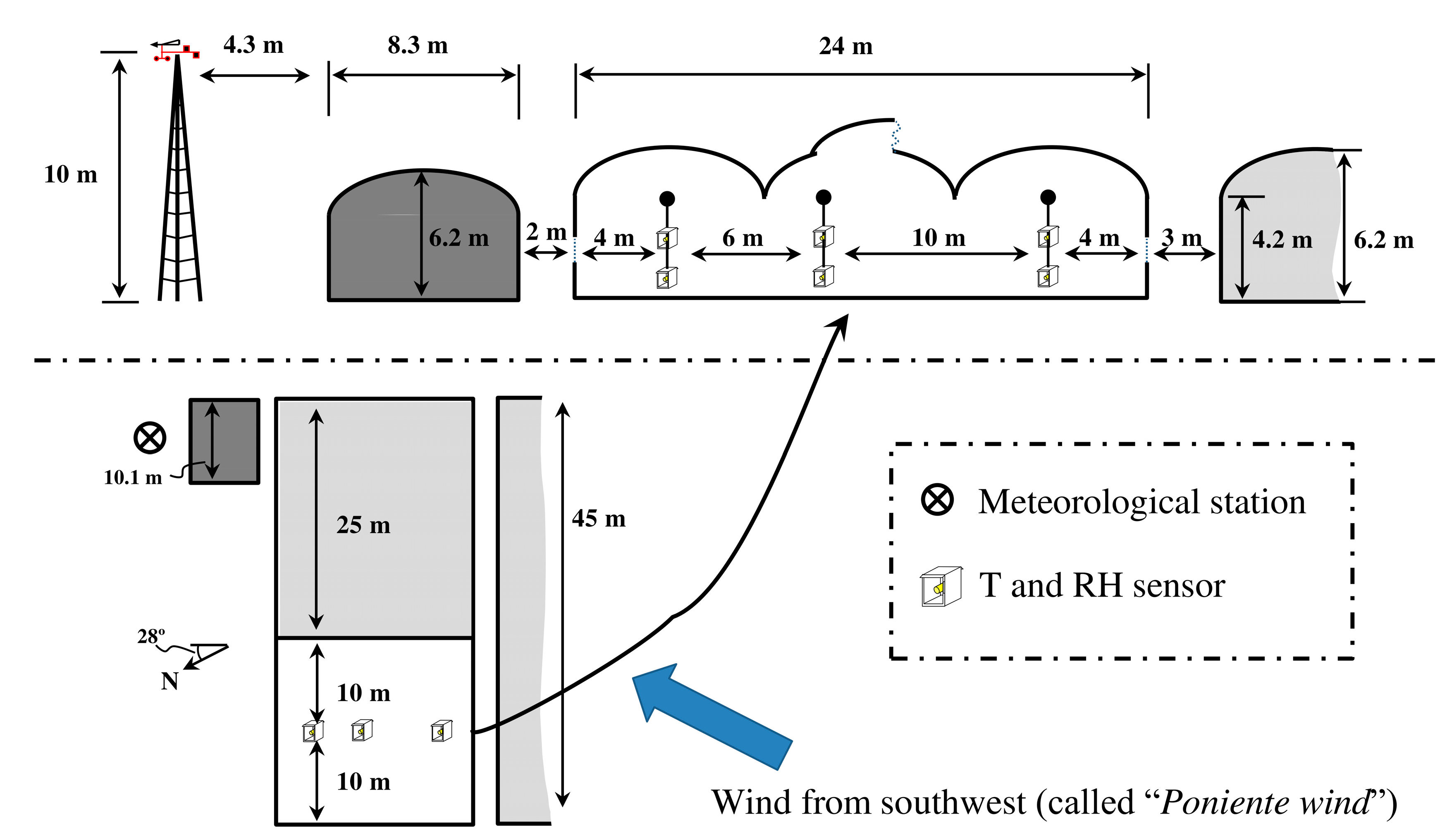
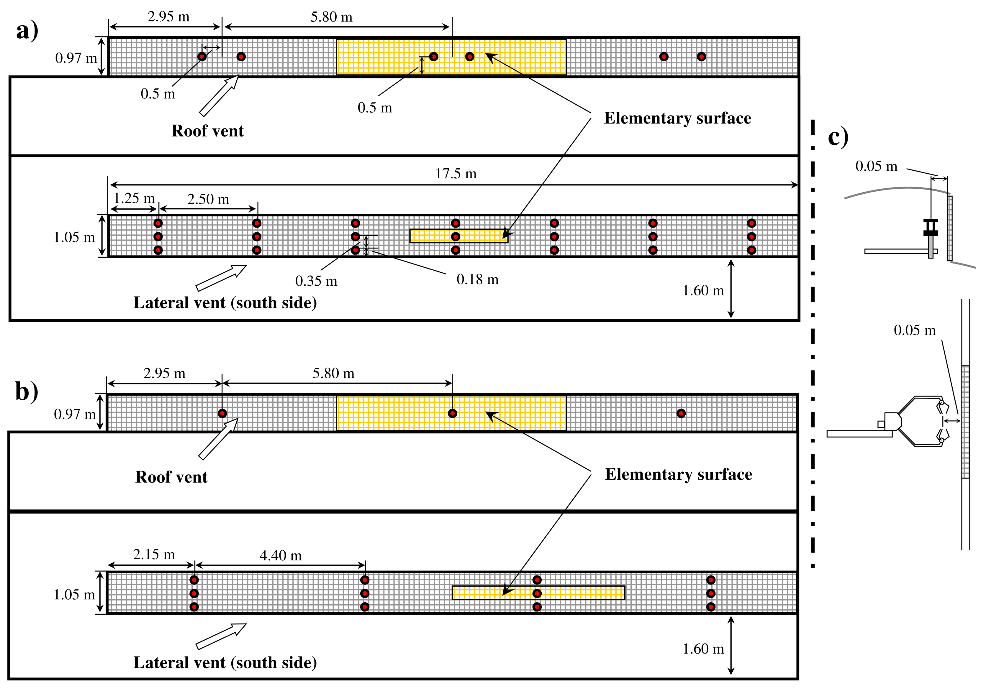
2.1. Experimental Setup

The experimental work took place in a three-span Mediterranean greenhouse (1080 m²) located at the agricultural research farm belonging to the University of Almería (36°51′ N, 2°16′ W, and 87 MASL). The greenhouse was divided into two independent halves (Figure 1). In this work, we studied the natural ventilation in the western half (24 × 20 m²), which has less obstruction to the wind.

In the western sector of the greenhouse, the vent surface area was 1.05 × 17.5 m² for each of the two-side vents (2.1 m in height from the ground to the mid-point of the vent) and 0.97 × 17.5 m² for the roof vent (6.2 m in height from the ground to the mid-point of the vent), and 4.1 m of vertical distance between the mid-point of the side and the roof vents. The ventilation surface S_V was 11.2% of the greenhouse base area (S_V/S_A = 0.112). To prevent insects entering, all the greenhouse vents were fitted with insect-proof screens of 13 × 30 threads cm⁻² (0.39 porosity; 164.6 µm pore width; 593.3 µm pore height; 165.5 µm thread diameter). Measurement tests were carried out under prevailing winds from the southwest (Figure 1), popularly known as “Poniente wind” (in the province of Almería). The outside climatic conditions remained relatively stable over the ten measurement tests (

Table 1. Outside climatic conditions for the measurement tests. Average wind speed u_o [m s⁻¹], wind direction θ [°], outside and inside temperature T_o and T_i [°C], outside and inside humidity RH_o and RH_i [%], outside radiation R_g [W m⁻²] and ratio determining the relative importance of the wind and thermal buoyancy forces u_o/∆T_io^0.5.

Test	Date	Time	uo	θa	RHo	RHi	To	Ti	Rg	uo/∆Tio0.5
1	07/04/2009	11:52–14:47	6.86 ± 1.41	300 ± 7	67 ± 2	52 ± 7	17.5 ± 0.4	22.8 ± 1.9	527 ± 259	2.98
2	08/04/2009	10:49–13:31	4.16 ± 1.06	295 ± 15	29 ± 8	38 ± 2	18.3 ± 0.4	25.7 ± 1.4	562 ± 237	1.53
3	14/04/2009	11:21–14:01	4.01 ± 1.13	294 ± 10	72 ± 2	57 ± 2	16.3 ± 0.6	23.7 ± 0.7	692 ± 108	1.47
4	07/05/2009	10:56–12:36	2.03 ± 0.84	264 ± 14	36 ± 3	60 ± 5	22.8 ± 0.7	27.6 ± 0.6	784 ± 60	0.93
5	17/04/2009	11:06–13:07	1.94 ± 0.70	226 ± 25	59 ± 5	53 ± 4	16.9 ± 0.4	25.7 ± 1.0	584 ± 175	0.65
6	23/04/2009	11:23–13:16	2.34 ± 0.98	267 ± 14	38 ± 2	55 ± 6	22.1 ± 0.6	28.3 ± 0.1	809 ± 56	0.94
7	22/06/2009	11:14–12:58	3.42 ± 0.50	258 ± 8	56 ± 4	70 ± 2	25.5 ± 0.4	27.2 ± 0.5	617 ± 71	2.57
8	26/06/2009	11:17–13:04	2.67 ± 0.72	227 ± 20	64 ± 2	73 ± 3	24.0 ± 0.5	28.2 ± 0.2	751 ± 102	1.29
9	02/07/2009	11:00–12:45	2.62 ± 0.63	239 ± 17	65 ± 3	76 ± 3	27.0 ± 0.9	30.8 ± 0.4	725 ± 68	1.34
10	02/07/2009	14:41–16:28	3.22 ± 0.48	242 ± 14	60 ± 2	69 ± 2	28.0 ± 0.8	32.1 ± 0.5	868 ± 37	1.58

^a Direction perpendicular to the roof window at windward is 208° for a southwest wind (SW).

). The greenhouse contained a tomato crop (Solanum lycopersicum L. var. cerasiforme Hort., cv. Salomee) with an average height of approximately 0.85 m for the first test and 1.88 m for the final one, and a leaf area index (m² leaf per m² ground.) of about 0.37 and 2.75, respectively. The measurements were performed from 7 April 2009 to 2 July 2009.

Airflow was measured at 21 points (tests 1 to 4) and 12 points (tests 5 to 10), evenly distributed at the side vents (Figure 2a,b). To measure air velocity at the side vents, two 3D sonic anemometers were used (Figure 2c), recording data over three minutes at each point [19].

Given the difficulty of placing the sonic anemometers in the roof vent, it was divided into three equal surfaces and air velocity measurements were taken continuously at the centre of each one, with two (measurement tests 1 to 4) or one (measurement tests 5 to 10) 2D sonic anemometers (Figure 2a,b). At the roof vent, these measurements were taken continuously using six (tests 1 to 4) or three (tests 5 to 10) 2D sonic anemometers (Figure 2c).

The distribution of measurement points used in the present study was very similar to the one made in Espinoza et al. [24], in the same experimental greenhouse. For lateral vents, the surface corresponding to each point was 0.9 m² (tests with 21 points) and 1.5 m² (tests with 12 points). These are similar values to those used by other authors. Boulard et al. [25] used 2.6 m² per point in a tunnel greenhouse with one roof vent, Teitel et al. [18] used 1.1 m² per point in a mono-span greenhouse with two side vent openings, and Molina-Aiz et al. [19] used 2.1 m² per point in a five-span Almería-type greenhouse. At the roof vent, the mean surface corresponding to each section was 5.8 m². Teitel et al. [26] used a larger surface area for each measurement point, with 8.5 m² per point in a four-span greenhouse with three roof vents.

2.2. Equipment and Instrumentation

The three components of air velocity and air temperature were measured with two 3D sonic anemometers. The horizontal components of air velocity (x and y) were measured with six 2D sonic anemometers (

Table 2. Sensors used and their specifications.

Type	Model	Manufacturer	Measurements	Measurement Range	Resolution	Accuracy
3D sonic Anemometer	CSAT3	Campbell Scientific Spain S.L	Air velocity (ux, uy and uz) and air temperature	0–30 m s−1 −30–50 °C	0.001 m s−1 0.002 °C	±0.001 m s−1 ±0.002 °C
2D sonic Anemometer	Windsonic	Gill Instrument LTD	Air velocity (ux and uy)	0–60 m s−1 0–359°	0.01 m s−1 1°	2% 3°
Temperature Pt1000 and capacitive humidity sensor	BUTRON II	Hortimax S.L.	Air temperature and humidity	−25–75 °C 0–100%	0.01 °C 1%	±0.01 °C ±3%
Cup anemomer and vane	Meteostation II	Hortimax S.L.	Wind velocity Wind direction	0–40 m s−1 0–359°	0.1 m s−1 1°	±5% ±5%
Radiation sensor	Kipp Solari	Hortimax S.L.	Solar radiation	0–2000 W m−2	0.1 W m−2	±20 W m−2
Termistor and capacitive humidity sensor	HOBO Pro Temp-RH U23-001	Onset Computer Corp.	Air temperature and humidity	−40–75 °C 0–100%	0.02 °C 0.03%	±0.18 °C ±3%

). The data measured by the sonic anemometers were recorded by two CR3000 Microloggers (Campbell Scientific Spain S.L.). The data registration frequency was 10 Hz [27] for 3D sonic anemometers and 1 Hz for 2D sonic anemometers, respectively.

Outside climatic conditions were recorded by a meteorological station at a frequency of 0.5 Hz (Figure 1). It included a measurement box with a Pt1000 temperature sensor and a capacitive humidity sensor (BUTRON II). Wind speed and direction were recorded by a cup anemometer and a vane. Solar radiation was measured using a Kipp Solari sensor. Air temperature and humidity inside the greenhouse were measured using six autonomous dataloggers HOBO Pro Temp-RH U23-001 (Table 2). The dataloggers were placed in a vertical profile under the ridge of the three greenhouse spans at heights of 1 and 2 m (Figure 1). These autonomous dataloggers were protected against direct solar radiation with a passive solar radiation open shield.

2.3. Ventilation Models

In general, we can consider that the natural ventilation in a greenhouse is the result of combining two different fluxes: one generated by wind and the other generated by buoyancy forces. We can combine these fluxes and obtain different semi-empirical models based on Bernoulli’s equation [4,7,19,28]. These models (used by Molina-Aiz et al. [19]) can be modified by applied using a different discharge coefficient for the side vents (C_dVS) and for the roof vent (C_dVR):

(1)

Model 1. In this model, the flow is driven by the sum of two independent pressure fields. In a greenhouse with side and roof openings, G is calculated as the vector sum of the free component of the flux induced by buoyancy forces G_T and the flux induced by wind forces G_w:

$$G_{M1}=\sqrt{{\left(\frac{\left(C_{dVR}\times S_{VR}\right)\left(C_{dVS}\times S_{VS}\right)}{\sqrt{{\left(C_{dVR}\times S_{VR}\right)}^2+{\left(C_{dVS}\times S_{VS}\right)}^2}}\right)}^2\left(2g\frac{\Delta T_{io}}{T_o}{h}_{SR}\right)+{\left(\frac{C_{dVR}\times S_{VR}+C_{dVS}\times S_{VS}}{2}\right)}^2{C}_w\times u_o^2}$$

(1)

where S_VR and S_VS are the roof and side total vent areas, respectively [m²], g is the gravitational constant [m s⁻²], ∆T_io is the inside-outside temperature difference [K], T_o is the outside temperature [K], u_o is the outside wind speed [m s⁻¹], C_d is the discharge coefficient (C_dVR, roof vent; C_dVS, side vents), C_w is the wind effect coefficient, and h_SR is the vertical distance between the mid-point of the side and the roof vents [m].

(2)

Model 2. In this model, the flow is driven by the sum of two independent fluxes. The greenhouse volumetric flow rate is calculated as the algebraic sum of the free component of the flux induced by buoyancy forces G_T and the flux induced by wind forces G_w:

$$G_{M2}=\left[\frac{\left(C_{dVR}\times S_{VR}\right)\left(C_{dVS}\times S_{VS}\right)}{\sqrt{{\left(C_{dVR}\times S_{VR}\right)}^2+{\left(C_{dVS}\times S_{VS}\right)}^2}}\sqrt{2g\frac{\Delta T_{io}}{T_o}{h}_{SR}}+\frac{C_{dVR}\times S_{VR}+C_{dVS}\times S_{VS}}{2}\sqrt{C_w}{u}_o\right]$$

(2)

(3)

Model 3. In this model, only the wind effect is considered, neglecting the thermal effect:

$$G_{M3}=\frac{C_{dVR}\times S_{VR}+C_{dVS}\times S_{VS}}{2}\sqrt{C_w}{u}_o$$

(3)

The height of the meteorological station and its distance from the greenhouse condition the results obtained when applying the models. This aspect is important to keep in mind when applying the models described in the literature.

2.4. Anemometric Measurement of Volumetric Flow Rate

To describe the air circulation through the greenhouse vents, the mean and turbulent volumetric flow rates can be calculated considering only the component of air velocity perpendicular to the vent, u_x [25]:

$${\overline{G}}_j={\displaystyle \sum }_{j=1}^n\left(S_{V,j}\times u_{x,j}\right)$$

(4)

$$G_j^{\prime }={\displaystyle \sum }_{j=1}^n\left(S_{V,j}\times \left|u_{x,j}^{\prime }\right|\right)$$

(5)

where u_x,j are the time average value of air velocity perpendicular to the vent, |u’_x,j| are the time average value of the absolute values of the turbulent component, and S_V,j are elementary surface corresponding to each measurement point. With only two 3D sonic anemometers measuring at the lateral vents, at different intervals of 3 min (Figure 2), the external conditions can change or fluctuate during the test. This problem can be overcome by correcting (scaling with the wind speed) the air velocities measured at each position j at the lateral vents [19]. The corrected air velocity u^*_x,j(t) has been calculated by multiplying measured values of u_x,j(t), at time t and at each point j, by the ratio between the average wind speed u_o for the overall test period, and the measured values of u_o(t) at time t [19]:

$$u_{x,j}^{*}\left(t\right)=u_{x,j}\left(t\right)\frac{u_o}{u_o\left(t\right)}$$

(6)

2.5. Estimation of the Pressure Drop/discharge Coefficient of the Greenhouse Openings

The individual pressure drop coefficient of each vent C_d was determined following the methodology outlined by Molina-Aiz et al. [19]. Calculation of C_d requires knowing the specific permeability (K_p = 1.851·10⁻⁹) and inertial factor (Y = 0.155) of the insect-proof screens installed in the vents; these values were determined in wind-tunnel tests. A detailed description of the wind-tunnel experiment was provided by Valera et al. [29] or López et al. [30]. To determine K_p and Y, the thickness of the screen is required (e = 391.7 µm), which was obtained by measuring a transversal section of the net with an optical measurement unit equipped with a video system (TESA-VISIO 300, TESA SA, Switzerland; with a resolution of 0.05 μm and precision of ±7 μm).

2.6. Statistical Analysis

We carried out regression analyses to compare the different variables for statistically significant relationships (p-value < 0.05) using Statgraphics^®Centurion 18 v18.1 (Statgraphics Technologies, Inc., The Plains, VA, USA). In order to analyse the fit of the average volumetric flow rate for the greenhouse G_M,sim (simulated by models M1, M2 and M3) with the experimentally observed values of G_M,obs, different statistics were used, as well as the determining coefficient R². Two of the most commonly used statistics based on the deviation of G_M,sim from G_M,obs are RMSD (root mean squared deviation) and MD (or bias) [31]:

$$RMSD=\sqrt{\frac{1}{n}{\displaystyle \sum }_{i=1}^n{\left(G_{M,obs}-G_{M,sim}\right)}^2}$$

(7)

$$MD=\frac{1}{n}{\displaystyle \sum }_{i=1}^n\left(G_{M,obs}-G_{M,sim}\right)$$

(8)

RMSD represents the average distance between the simulated and observed values. MD corresponds to the mean value of the differences between the simulated and observed values, though in this case negative differences are compensated by positive ones, which may lead to erroneous interpretation. Both statistics represent different aspects of the deviation from simulated values, but the relationship between them has not been well defined [31]. The Nash-Sutcliffe efficiency (NSE) is a normalised statistic indicating the relative magnitude of the residual variance of the model (“noise”) with respect to the variance of the observed values (“information”) [32]. NSE indicates how well the plot of the observed versus simulated values fits the 1:1 line [33]:

$$NSE=1-\left[\frac{{{\displaystyle \sum }}_{i=1}^n{\left(G_{M,obs}-G_{M,sim}\right)}^2}{{{\displaystyle \sum }}_{i=1}^n{\left(G_{M,obs}-{\overline{G}}_{M,obs}\right)}^2}\right]$$

(9)

where ${\overline{G}}_{M,obs}$ is the average value of all the G_M,obs values. NSE can take values of between −∞ and 1.0, the latter being the optimal value. Values between 0.0 and 1.0 are generally viewed as acceptable levels of performance [33]. Percent bias PBIAS represents the mean trend of simulated values to greater or lower than their respective observed values [34]. The optimal value of PBIAS is 0.0, and values close to 0 indicate high precision of the model. Positive values indicate that the model provides values that are lower than those observed (model underestimation bias), while negative ones indicate the contrary (model overestimation bias) [34]. PBIAS can be expressed as a percentage:

$$PBIAS=\left[\frac{{{\displaystyle \sum }}_{i=1}^n\left(G_{M,obs}-G_{M,sim}\right)\times 100}{{{\displaystyle \sum }}_{i=1}^n\left(G_{M,obs}\right)}\right]$$

(10)

RMSD-observations standard deviation ratio (RSR): this statistic [33] was developed based on the recommendations of [35]. RSR standardises the values of RMSD with standard deviation from the observed values. It combines both an error index and the additional information recommended by Legates and McCabe [36]:

$$RSR=\frac{RMSD}{STDE{V}_{obs}}=\left[\frac{\sqrt{{{\displaystyle \sum }}_{i=1}^n{\left(G_{M,obs}-G_{M,sim}\right)}^2}}{\sqrt{{{\displaystyle \sum }}_{i=1}^n{\left(G_{M,obs}-{\overline{G}}_{M,obs}\right)}^2}}\right]$$

(11)

RSR takes values from 0 to a large positive value, and when RMSD is equal to zero, the model is considered perfect. Small values of RSR indicate a better performance of the simulation model [33].

3. Results and Discussion

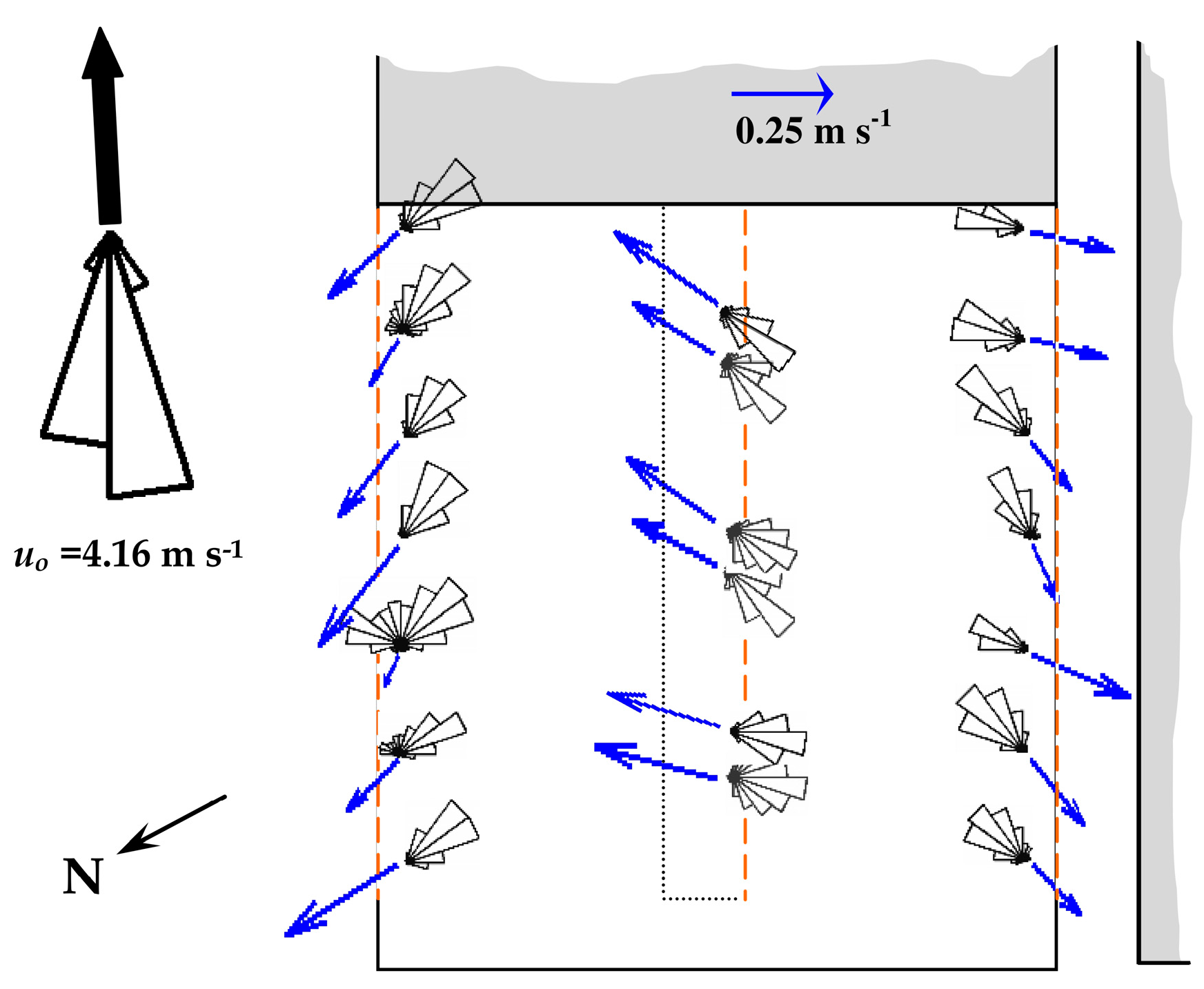
3.1. Airflow Inside the Greenhouse

Given the particular situation of the greenhouse and the location of the vents, in conditions of natural ventilation with prevailing southwest wind (SW) or “Poniente winds”, the eolic and thermal effects oppose each other. The former causes air to enter through the windward roof vent and to leave through the leeward and windward side vents (the windward side vent was protected from the wind by another greenhouse located in close proximity). The thermal effect, on the other hand, causes warm air to rise and leave through the roof vent, which favours the entrance of air through the side vents. Figure 3a,b shows the entrance and exit of air through the roof vent (see the polar histograms), demonstrating the negative interaction of the wind and thermal effects. This flow pattern with opposition of the wind effect and thermal effect in the roof vents, in the same naturally-ventilated three-span Mediterranean greenhouse, was described in more detail, including measurements among the crop lines, in López et al. [37]. And, similar flow patterns, in the same greenhouse and with the same methodology, was described in Espinoza et al. [24], opening the lateral vents combined with two and three roof vents.

The greenhouse natural ventilation rate is affected by the thermal effect due to the inside-outside temperature difference, ∆T_io. For greenhouses with side and roof vents, Kittas et al. [4] established that the thermal effect is important when the ratio u_o/∆T_io^0.5 < 1, while Bot [21] put this limit at 0.3. In tests 1, 2, 3, 7, and 10, with u_o/∆T_io^0.5 ≥ 1.5, hardly any air left the greenhouse through the roof vent, indicating that the wind effect clearly prevailed over the thermal effect, and the air left in quite a uniform fashion through the side vents (Figure 4).

In the other tests, with u_o/∆T_io^0.5 < 1.5, the opposing wind and thermal effects gave rise to less uniformity of air flow at the ventilation surfaces (Figure 3a,b), with alternating positive (entrance) and negative (exit) airflow at the roof vent (see polar histograms). In some of the tests, there was a certain degree of discrepancy between the wind direction and the airflow direction entering the greenhouse through the roof vent. This is likely due to the location of the meteorological station, to the north of the greenhouse, which therefore recorded the wind characteristics once it had passed through the experimental greenhouse.

3.2. Evaluation of the Mean and Turbulent Ventilation Flows

The longitudinal component u_x at the side vents is corrected according to Equation 6 to compensate for the change in wind speed during the tests. This did not prove necessary for the roof vent, as the measurements were taken continuously (

Table 3. Average values of the u_x component of the air velocity perpendicular to the greenhouse vents and the corrected u_x^*. LS, leeward side vent; WS, windward side vent; WR, windward roof vent.

Test Number	ux, [m s−1]			ux*, [m s−1]
	LS	WS	WR	LS	WS
1	−0.42 ± 0.13	−0.29 ± 0.11	0.83 ± 0.29	−0.42	−0.29
2	−0.14 ± 0.06	−0.14 ± 0.06	0.30 ± 0.09	−0.14	−0.15
3	−0.17 ± 0.06	−0.16 ± 0.07	0.27 ± 0.04	−0.18	−0.17
4	0.03 ± 0.04	−0.11 ± 0.05	0.07 ± 0.02	0.03	−0.11
5	−0.02 ± 0.06	−0.08 ± 0.06	0.09 ± 0.03	−0.01	−0.08
6	−0.01 ± 0.06	−0.12 ± 0.08	0.11 ± 0.02	0.02	−0.11
7	−0.09 ± 0.07	−0.17 ± 0.05	0.25 ± 0.06	−0.08	−0.17
8	0.01 ± 0.08	−0.15 ± 0.05	0.12 ± 0.05	0.03	−0.14
9	0.00 ± 0.06	−0.11 ± 0.04	0.11 ± 0.05	−0.01	−0.11
10	−0.06 ± 0.13	−0.14 ± 0.03	0.17 ± 0.05	−0.06	−0.14

Positive values for an inflow and negative values for an outflow.

).

By applying Equations (4) and (5), we determined the volumetric flow rates at the three greenhouse vents. Knowing the volumetric flow rate of the greenhouse, G_M allows the ventilation rate R_M to be calculated (

Table 4. Average values G (Equation (8)) and turbulent component G’ (Equation (9)) of the ventilation volumetric flow rates through each vent opening. Error in the calculation of ventilation volumetric flow rates E_G and average values of ventilation rate R. LS, leeward side vent; WS, windward side vent; WR, windward roof vent; M, average values for the greenhouse.

Test	GLS [m3 s−1]	GWS [m3 s−1]	GWR [m3 s−1]	GM [m3 s−1]	EG, [%]	G’LS [m3 s−1]	G’WS [m3 s−1]	G’WR [m3 s−1]	RM [h−1]
1	−7.8	−5.3	14.1	13.6	7.5	4.1	4.0	8.2	18.2
2	−2.6	−2.7	4.0	4.6	−27.8	2.2	1.9	4.0	6.2
3	−3.3	−3.2	4.6	5.5	−33.6	2.6	2.3	4.0	7.4
4	0.6	−2.0	1.2	1.9	−11.4	1.7	1.2	2.6	2.6
5	−0.1	−1.5	1.59	1.6	1.8	2.1	1.8	3.0	2.1
6	0.3	−2.0	1.94	2.1	12.3	1.6	1.3	2.9	2.8
7	−1.5	−3.1	4.30	4.4	−6.2	1.6	1.3	3.3	6.0
8	0.5	−2.6	2.03	2.6	−5.3	1.8	1.2	3.3	3.5
9	−0.2	−2.0	1.80	2.0	−20.8	1.4	1.0	3.0	2.7
10	−1.2	−2.6	2.93	3.3	−24.3	1.9	1.3	3.4	4.5

Positive values for an inflow and negative values for an outflow.

and Figure 5a).

The precision of the mean values of G_M can be assessed by comparing them with the inflow and outflow volumes measured at the different ventilation surfaces. To verify the degree of satisfaction of the Mass Conservation Law in the greenhouse [1,28], the error in the calculation of the ventilation volumes has been estimated as follows:

$$E_G=\frac{\Delta G}{G_M}=\frac{G_{LS}\left(u_x^{*}\right)+G_{WS}\left(u_x^{*}\right)+G_{WR}\left(u_x\right)}{G_M}\times 100$$

(12)

If we calculate the airflow without correcting the inside air velocity with the outside wind speed, we obtain a mean error for all the assays of E_G = 17.2%, but on correcting it, the mean error of the assays is reduced to E_G = 15.1%. Following a similar methodology in an Almería greenhouse with two side and two roof vents, Molina-Aiz et al. [19] obtained errors of E_G between 3.0% and 37.0% (calculating airflows with u_x^*) and between 8.4% and 70.5% (with u_x). In a multi-tunnel greenhouse with a roof vent, other authors obtained errors of 2.2% and 2.6% [1], and of 31.6% [28].

The accuracy of the method of calculating the ventilation volumetric flow rates will depend mainly on the stability of the wind conditions (intensity and direction) and on the influence of the thermal effect on greenhouse ventilation. When wind conditions are not stable or when the dominance of the thermal effect or the wind effect is not clear, a greater degree of error should be expected. Maximum error was recorded in the assays for which the ratio u_o/∆T_io^0.5 was close to 1.5 (Figure 5b).

The greenhouse ventilation rate R_M under conditions of natural ventilation (Table 4) presents a better fit to a second order polynomial with the air velocity (R_M = 0.37 u_o² + 0.03 u_o +0.75; R² = 0.99 and p-value = 0.0000) (Figure 5a). Many authors present linear fits between wind velocity and the ventilation rate [4,7,18]. If the fit is carried out in this way, the R² coefficient obtained is somewhat lower (R_M = 3.20 u_o – 5.04; R² = 0.95 and p-value = 0.0000) and the resulting straight line would cross the abscissa at u_o = 1.61 m s⁻¹ (Figure 5a). According to this fit, for air velocity below this value, there would be no exchange of air with the outside, and so this cannot be considered a valid fit.

3.3. Application of the Semi-empirical Ventilation Models Based on Bernoulli’s Equation

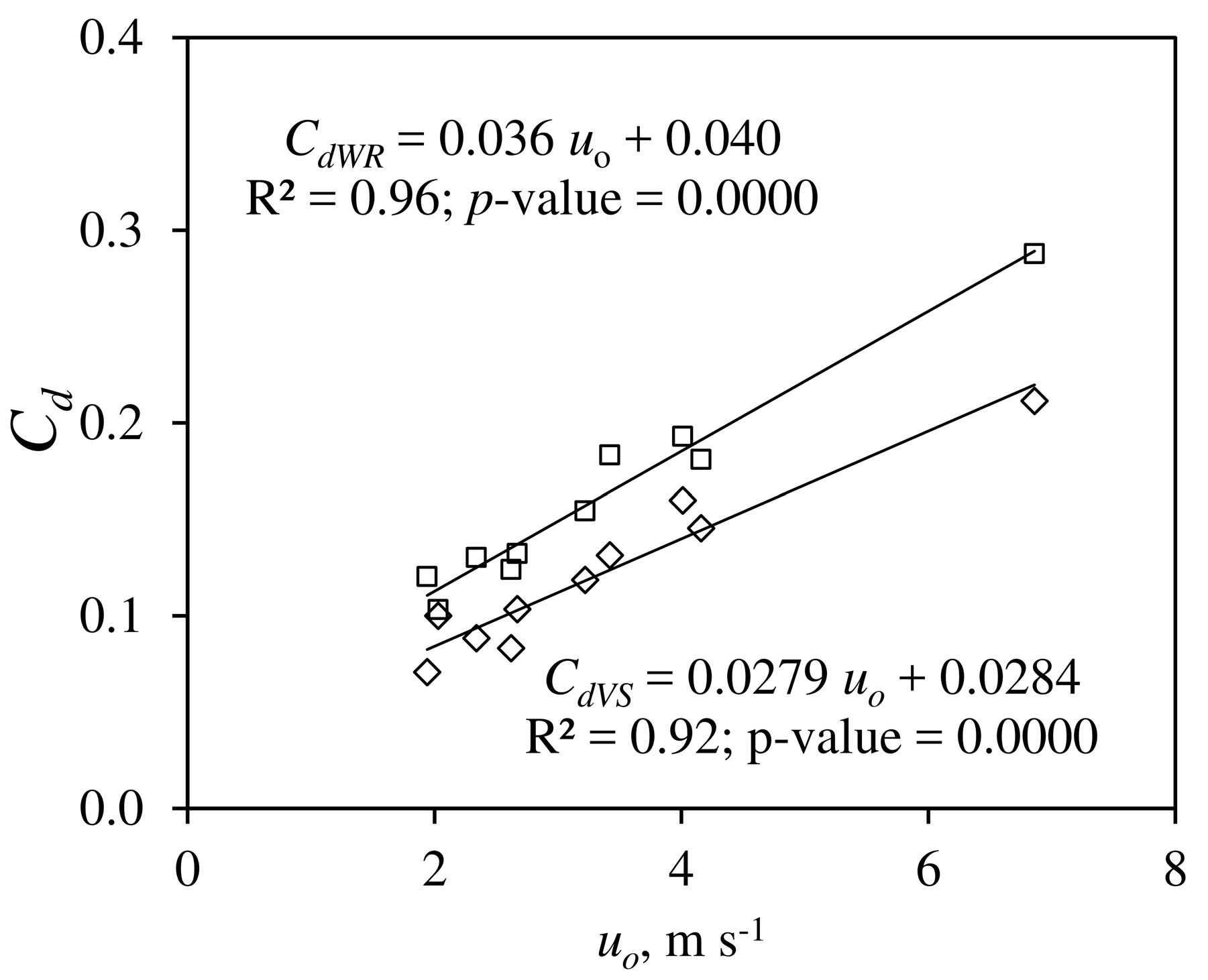
3.3.1. Determining the Discharge Coefficient of the Vents C_d

The discharge coefficients (

Table 5. Discharge coefficients obtained at the vents of the experimental greenhouse. C_dLS, leeward vent; C_dWS, windward vent; C_dVS, average coefficient for side vents; C_dWR, windward roof vent.

Test	CdLS	CdWS	CdVS	CdWR
1	0.227	0.196	0.211	0.288
2	0.144	0.147	0.145	0.181
3	0.161	0.158	0.160	0.193
4	0.073	0.127	0.100	0.103
5	0.030	0.111	0.071	0.120
6	0.050	0.126	0.088	0.130
7	0.110	0.153	0.131	0.183
8	0.063	0.143	0.103	0.132
9	0.040	0.126	0.084	0.124
10	0.097	0.140	0.119	0.154
Average	0.100 ± 0.062	0.143 ± 0.023	0.121 ± 0.042	0.161 ± 0.054

) have been obtained for each of the vents, following the methodology outlined by Molina-Aiz et al. [19]. The windward roof vent had the highest average discharge coefficient (C_dWR = 0.161 ± 0.054), followed by the windward side vent (C_dWS = 0.143 ± 0.023), and finally the leeward side vent (C_dLS = 0.100 ± 0.062); the average discharge coefficient for both side vents was C_dVS = 0.121 ± 0.042. The discharge coefficients of side vents C_dVS and of roof vent C_dWS can be expressed as a function of air velocity [C_dVS = 0.028·u_o + 0.028 (R² = 0.92 and p-value = 0.0000); C_dWR = 0.036·u_o + 0.040 (R² = 0.96 and p-value = 0.0000)] (Figure 6).

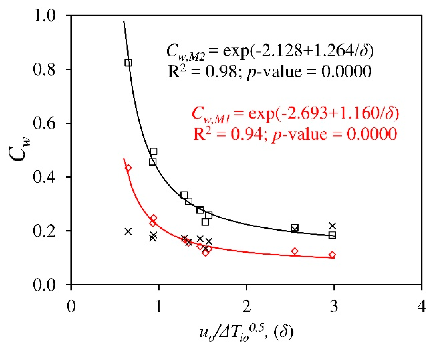
3.3.2. Determining the Wind Effect Coefficient C_w

Once the discharge coefficient of the greenhouse vents, C_dVS and C_dWR (Table 5), and the average volumetric flow rate, G_M, are known (Table 4), we can calculate the wind effect coefficients C_w for each of the experiments (

Table 6. Wind effect coefficients C_w obtained for the experimental greenhouse according to the original ventilation models M1, M2, and M3 (Equations (1), (2) and (3)) and the modified models M1 and M2 (Equations (13) and (14)). E_v, coefficient of the effectiveness of the opening E_v = C_dM C_w^0.5 based on model M3.

Test	Cw					Ev
	Original		Modified		M3	M3
	M1	M2	M1	M2
1	0.085	0.039	0.111	0.184	0.218	0.110
2	0.023	0.002	0.117	0.233	0.134	0.087
3	0.041	0.006	0.141	0.277	0.171	0.052
4	0.015	0.000	0.228	0.455	0.173	0.064
5	−0.188	0.043	0.433	0.824	0.198	0.038
6	−0.030	0.002	0.248	0.494	0.184	0.044
7	0.089	0.037	0.124	0.211	0.204	0.101
8	0.035	0.004	0.168	0.333	0.173	0.035
9	0.021	0.001	0.155	0.309	0.158	0.058
10	0.044	0.007	0.133	0.258	0.161	0.079
Average	0.013 ± 0.079	0.014 ± 0.018	0.186 ± 0.098	0.358 ± 0.192	0.177 ± 0.025	0.060 ± 0.023

).

This dimensionless wind effect coefficient expresses the relationship of the field of velocities measured on a reference level (the meteorological station) and on another level close to the greenhouse vents [2].

Equations (1)–(3) have been used to obtain C_w in accordance with the three models of ventilation, M1, M2, and M3, respectively, derived from Bernoulli’s equation [4,7,10]. Ventilation models M1 and M2 consider that the wind and thermal effects complement each other. However, this does not always occur, and Li and Delsante [22] considered two situations: “fully assisting and fully opposing”. According to these authors, the latter can occur when there are only two ventilation openings. Although the greenhouse in the present study has three ventilation openings, the ventilation models present a better fit considering the fully opposing scenario (subtracting the wind and thermal effect) than considering the fully assisting scenario (adding the wind and thermal effect). It is necessary to modify models M1 and M2 so as to indicate the relationship between the two effects:

$$G_{M1}=\sqrt{\left|G_T^2\pm G_w^2\right|}=\sqrt{\left|{\left(\frac{\left(C_{dVR}\times S_{VR}\right)\left(C_{dVS}\times S_{VS}\right)}{\sqrt{{\left(C_{dVR}\times S_{VR}\right)}^2+{\left(C_{dVS}\times S_{VS}\right)}^2}}\right)}^2\left(2g\frac{\Delta T_{io}}{T_o}{h}_{SR}\right)\pm {\left(\frac{C_{dVR}\times S_{VR}+C_{dVS}\times S_{VS}}{2}\right)}^2{C}_w{u}_o^2\right|}$$

(13)

$$G_{M2}=\left|G_T\pm G_w\right|=\left|\frac{\left(C_{dVR}\times S_{VR}\right)\left(C_{dVS}\times S_{VS}\right)}{\sqrt{{\left(C_{dVR}\times S_{VR}\right)}^2+{\left(C_{dVS}\times S_{VS}\right)}^2}}\sqrt{2g\frac{\Delta T_{io}}{T_o}{h}_{SR}}\pm \frac{C_{dVR}\times S_{VR}+C_{dVS}\times S_{VS}}{2}\sqrt{C_w}{u}_o\right|$$

(14)

Equation (13) is similar to that proposed by Li and Delsante [22]. Table 6 shows the wind coefficients obtained with the original models M1 and M2 (Equations (1) and (2)) and with the modified models (Equations (13) and (14)). When we do not consider the appropriate relationship between the wind and thermal effects, very low wind effect coefficients are obtained, and even negative coefficients are found in some of the experiments for model M1 (Table 6).

To optimise the proposed ventilation models, it would be necessary to evaluate the real relationship between the two effects in each specific situation. The two simplest scenarios are those studied by Li and Delsante [22], “fully assisting and fully opposing”, and we understand that the latter occurs in our greenhouse. In commercial greenhouses with more than three ventilation surfaces, an intermediate situation can occur, making it difficult to determine an appropriate model.

In Espinoza et al. [24], the flow patterns were determined in the east sector of the experimental greenhouse (Figure 1), opening 2 lateral vents combined with 2 or 3 roof vents (making a total of 4 or 5 vents). In the windward roof vent, opposition of the wind effect and thermal effect was observed, but in the leeward roof vent, these two effects were added. By combining windward and leeward roof vents in the greenhouse, an intermittent situation between “fully assisting and fully opposing” would take place.

Table 6 and Figure 7 illustrate how the coefficient C_w obtained by model M3 (which ignores the thermal effect) maintains relatively similar values for the different tests (between 0.134 and 0.218). This means that a mean value of C_w can be considered for model M3 to predict the ventilation rate according to wind velocity, as has been done in previous research works [10,12,13,15,17,18,19]. However, the same does not apply to models M1 and M2, in which the thermal effect is taken into account in the equations (and with a wind effect opposition). For model M1, the coefficient C_w, obtained by applying Equation (13), takes values of between 0.111 and 0.433; while for model M2, applying Equation (14), it takes values of between 0.184 and 0.824 (Figure 7). This variation in C_w when applying models M1 and M2 was also observed in an Almería-type greenhouse with two side vents and two roll-up roof vents [38]. The values of C_w for models M1 and M2 have been seen to vary according to the ratio u_o/∆T_io^0.5 (Figure 7).

Low values of the ratio u_o/∆T_io^0.5 would indicate that the thermal effect has a major bearing on natural ventilation of the greenhouse. In this case, since the thermal and wind effects are opposing, on applying models M1 and M2, higher values of C_w are obtained, possibly to compensate for the strong opposition of the two effects.

High values of the ratio u_o/∆T_io^0.5 would indicate that the thermal effect has less bearing on natural ventilation and that the wind effect predominates. In this case, by applying models M1 and M2, the C_w values obtained are close to those obtained by model M3 (Figure 7), which ignores the thermal effect. It has been observed that the C_w coefficient that corresponds to each test can be calculated according to the ratio u_o/∆T_io^0.5 or δ [C_w,M1 = exp(−2.693 + 1.160/δ) (R² = 0.94 and p-value = 0.0000); C_w,M2 = exp(−2.128+1.264/δ) (R² = 0.98 and p-value = 0.0000)] (Figure 7). Kittas et al. [2] observed how this coefficient increased at low air velocities in a tunnel greenhouse with continuous side openings.

Although models M1, M2, and M3 can be used in their current form to predict the greenhouse ventilation rate, as is explained below, more work is required to ascertain the dependence of C_w on the ratio u_o/∆T_io^0.5 for models M1 and M2.

Using the original models M1 and M2, the mean values of C_w are 0.013 ± 0.079 (M1) and 0.014 ± 0.018 (M2) (Table 6), which are much lower than those obtained by other authors (

Table 7. Values of the wind effect coefficient C_w, discharge coefficient of the openings C_d, coefficient of effectiveness of the openings E_v = C_d C_w^0.5 obtained by different authors in different types of greenhouses with side and roof vents, with and without insect-proof screens (all values are taken from Molina-Aiz et al. [19]). S_A, greenhouse base surface area [m²]; u_o, air velocity [m s⁻¹]; M, model used.

M	Cw		Ev		Cd	Greenhouse Type	Method *	SA	uo	Source
Without Insect-Proof Screens
M1	0.079		0.210		0.754	Multi-span	Gas	416	0–8	[11]
M1	0.09		0.204		0.68	Multi-span	Gas	416	0–8	[4]
M1	0.098		0.175		0.56	Multi-span	Gas	242	1–3	[14]
M1	0.103 a		0.210		-	Multi-span	Gas	179	0.5–2.7	[16]
M1	0.116		0.303		0.89	Multi-span	Gas	242	1–3	[14]
M1	0.12		0.208		0.6	Tunnel	Gas	416	2	[2]
M1	0.13		0.252		0.7	Multi-span	Gas	416	0–8	[4]
M2	0.1		0.178		0.42	Multi-span	Gas	416	0–8	[4]
M3	0.012 a		0.07–0.18		-	Tunnel	Gas	240	1–2	[10]
M3	0.04 a		0.131		-	Tunnel	Om	368	5	[15]
M3	0.085 a		0.190		-	Multi-tunnel	Gas	416	5.3	[10]
M3	0.173 a		0.270		-	Multi-span	Gas	10000	2–4	[12]
M	φ	Cw		Ev	Cd	Greenhouse Type	Method *	SA	uo	Source
With Insect-Proof Screens
M1	0.34	0.048		0.043	0.194	Almería	3D	1694	5.71	[19]
M2	0.34	0.021		0.028	0.194	Almería		1694	5.71	[19]
M3	0.34	0.066		0.050	0.194	Almería		1694	5.71	[19]
M3	0.5	0.022 a		0.096	-	Single tunnel	Gas	160	2.2	[17]
M3	0.35	0.071		0.069	0.253	Single tunnel	Gas/H2O/3D	74.4	4.5	[18]
M3	0.69	0.110		0.140	0.42	Canary	Gas	5600	1-2	[13]

φ, porosity of the insect-proof screens; S_A, greenhouse base surface area; ue, air velocity. ^a, wind effect coefficient Cw calculated using C_d = 0.65 (the discharge coefficient of the openings was not indicated by these authors). * Method: Gas (N₂O tracer gas), H₂O (Mass balance on water vapour), 3D (trisonic anemometer), Om (omnidirectional hot-ball anemometer).

). On applying the modified ventilation models, these values are 0.186 ± 0.098 (M1) and 0.358 ± 0.192 (M2), which are closer to the values found by other researchers in multi-span type greenhouses and are considerably higher than those found by Molina-Aiz et al. [19] in an Almería-type greenhouse (Table 7).

The use of sonic anemometry has allowed us to observe the negative interaction between wind and thermal effects in the experimental greenhouse. Other techniques, such as the tracer gas method, allow correct quantification of the ventilation rates in the greenhouse, but they provide no information on the characteristics of the airflow [1], nor do they allow us to determine the way in which the two effects interact. Had the tracer gas method been used, applying the original ventilation methods would give much lower wind effect coefficients than those obtained taking into account the correct relationship between the wind and thermal effects. The wind effect coefficients obtained by other authors using the tracer gas method (Table 7) may be affected by a negative interaction between the two effects.

Since M3 does not consider the thermal effect, in general, lower wind effect coefficients are obtained (Table 6) than with models M1 and M2. Model M3 includes the thermal effect in the wind effect coefficients, and as the relationship between both effects is negative, lower wind effect coefficients are obtained than when the two effects are treated separately. Model M3 assumes that the volumetric caudal of air in a greenhouse is proportional to: the surface area of the vents S_V, the air velocity u_o, and the coefficient of effectiveness of the openings E_v = C_d·C_w^0.5. The latter is frequently used in the literature to characterise the wind effect in the ventilation of greenhouses [19]. The present study has used a different expression in model M3 to that used by Molina-Aiz et al. [19]; rather than the coefficient C_d and the total vent surface area S_V, this study opts for the coefficients corresponding to the side vents C_dVS, to the roof vent C_dWR, and their corresponding surfaces. In our case, the coefficient E_v of the vents has been obtained by calculating C_d as the weighted average value between C_dVS and C_dWR, according to the surface of each vent.

The coefficients of effectiveness obtained in the present work with M3 (Table 6), in some tests, are lower than those obtained by other authors in greenhouses with side and roof vents, and with insect-proof screens (Table 7), possibly due to the negative interaction between the wind and thermal effects in our greenhouse.

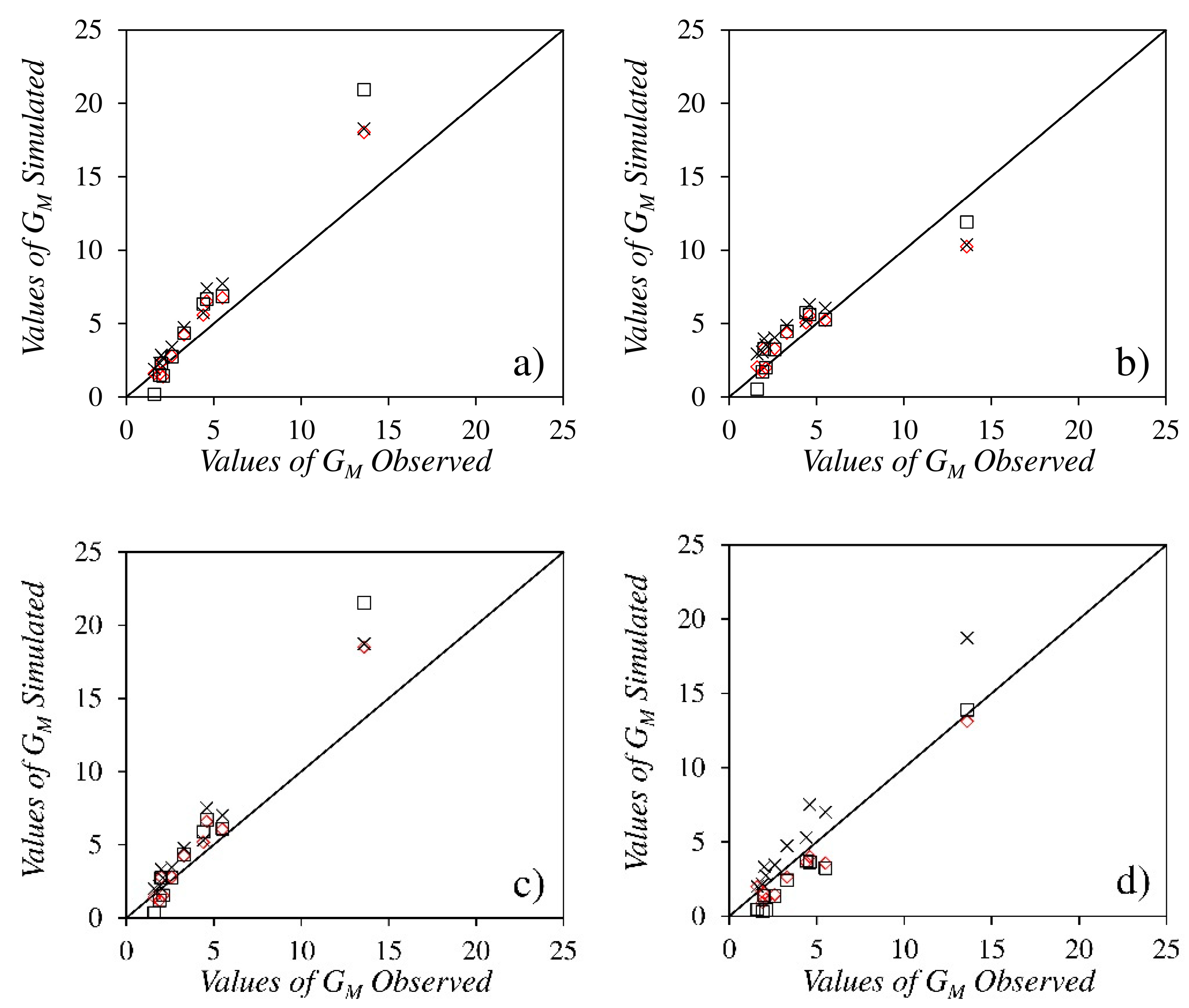
3.3.3. Fitting the Semi-Empirical Models to Experimental Data

To assess the fit of the three models with the experimental values, the flow rates were obtained for each experiment applying the three models. These ventilation flow rates have been estimated by applying the ventilation models in four ways (Figure 8): (i) first, using the mean wind coefficient C_w (0.186 for M1, 0.358 for M2 and 0.177 for M3) and the particular discharge coefficients, C_dVS and C_dWR, for each test (Table 5); (ii) second, using the mean wind coefficient C_w (idem) and the mean discharge coefficients C_dVS and C_dWR (equal to 0.121 and 0.161, respectively); (iii) third, using the mean wind coefficient C_w (idem) and the fits C_dVS = 0.028·u_o + 0.028 and C_dWR = 0.036·u_o + 0.040; (iv) fourth, also using the fits C_w,M1 = exp(−2.693 + 1.160/δ) and C_w,M2 = exp(−2.128 + 1.264/δ).

Based solely on the determining coefficient R², in the former case, the three models show a very good fit with the experimental data (with R² = 0.992 for M1 and M3, R² = 0.991 for M2).

In the second case, model M3 best fits the experimental data with R² = 0.952, followed by M1 with R² = 0.925, and finally M2 with R² = 0.919. Applying the models with the fits C_dVS(u_o) and C_dWR(u_o) improves the fit of models M1 and M2 (R² = 0.986) and of M3 (R² = 0.987). Applying the models with the fits C_w,M1(δ), C_w,M2(δ), C_dVS(u_o), and C_dWR(u_o), the values of R² go down slightly for models M1 and M2 (R² = 0.973 for M1 and R² = 0.980 for M2). In Molina-Aiz et al. [19], the models that obtain a better fit to the experimental data are Model M1 (R² = 0.984), considering the resulting pressure distribution as the sum of the pressure fields due to stack and wind effects, and the most simplified M3 (R² = 0.985). In the case of Molina-Aiz et al. [19], the relationship between wind and thermal effects was “fully assisting”, with two side vents (one to windward and one to leeward) and two roll-up roof vents; the air entered through the side vents to exit through the roof vents.

Analysis based solely on the coefficient R² may give the impression that the behaviour of the three models is very good, given the high R² values obtained in all cases. On comparing the simulated and observed G_M values one by one (Figure 8), the simulated values are seen to vary considerably from the observed ones in certain cases.

Table 8. Statistical parameters obtained for the average volumetric flow rate for the greenhouse G_M,sim (simulated with the different models M1, M2 and M3) with the experimentally observed values G_M,obs. R², determining coefficient; RMSD, root mean squared error; MD, bias; NSE, the Nash-Sutcliffe efficiency; PBIAS, percent bias; RSR, RMSD-observations standard deviation ratio. Applying the models with mean values of C_w and the particular discharge coefficients C_dVS and C_dWR for each test (Application i), with mean values of C_w, C_dVS and C_dWR (Application ii); with mean values of C_w and the fits C_dVS(u_o) and C_dWR(u_o) (Application iii); with fits C_w,M1(δ), C_w,M2(δ), C_dVS(u_o) and C_dWR(u_o) (Application iv).

	Application i			Application ii
	M1	M2	M3	M1	M2	M3
R2	0.992	0.991	0.992	0.925	0.919	0.952
RMSD	1.7	2.6	2.0	1.3	1.0	1.7
RMSD (%)	40	62	48	31	24	40
MD	−0.9	−1.2	−1.5	−0.1	−0.2	−0.9
NSE	0.8	0.4	0.7	0.9	0.9	0.8
PBIAS	−22.0	−28.0	−36.9	−2.7	−5.1	−21.0
RSR	1.6	2.5	1.9	1.2	1.0	1.6
	Application iii			Application iv
	M1	M2	M3	M1	M2	M3
R2	0.986	0.986	0.987	0.973	0.980	0.987
RMSD	1.8	2.7	2.1	0.9	1.3	2.1
RMSD (%)	42	65	50	23	30	50
MD	−0.9	−1.2	−1.5	0.8	1.1	−1.5
NSE	0.7	0.4	0.6	0.9	0.9	0.6
PBIAS	−20.7	−27.7	−36.9	18.4	25.9	−36.9
RSR	1.7	2.6	2.0	0.9	1.2	2.0

presents the different statistics obtained for the three models, M1, M2, and M3, and the four different applications of the coefficients C_w, C_dVS, and C_dWR (Applications i, ii, iii and iv in Table 8). With model M3, higher values of G_M are obtained than those observed experimentally, irrespective of how the coefficients are applied (Figure 8), always obtaining values of PBIAS<0 (model overestimation bias). Models M1 and M2 present values of PBIAS<0 (model overestimation bias) for the first three applications of the coefficients (i, ii, and iii in Table 8) and values of PBIAS>0 (model underestimation bias) on applying the models using the fits C_w,M1(δ), C_w,M2(δ), C_dVS(u_o), and C_dWR(u_o). For the remaining statistics obtained, no great differences are observed between the different applications of the coefficients C_w, C_dVS, and C_dWR (Applications i, ii, iii and iv in Table 8). We consider the best application of the models uses the fits obtained for C_dVS and C_dWR as a function of u_o (for models M1, M2, and M3), and the fits obtained for C_w as a function of the ratio u_o/∆T_io^0.5 (for models M1 and M2). In this way, the values of the coefficients applied are closest to the values obtained experimentally.

In summary, model M3 considers a linear relationship between the wind velocity and the ventilation volumetric flow rates G_M, a statistical device which improves the quality of the fit, and which therefore must be used and interpreted with great care [39]. It has also been observed that the ventilation rate fits better a second order polynomial than a linear relationship with air velocity. We therefore recommend using the modified model M1, since it includes both the wind and thermal effects and it is the one with the greatest physical foundation, as it combines the pressure fields rather than the flow rates [4,7]. For model M1, the lowest values of RMSD and RSR are obtained when applying the model using the fits C_w,M1(δ), C_w,M2(δ), C_dVS(u_o), and C_dWR(u_o) (Application iv in Table 8), rather than Applications i, ii, and iii. Moreover, before applying the model, it is essential to determine whether the interaction between the wind and thermal effects is positive or negative.

In view of the results obtained in this work, we recommend to experimentally determine the coefficients C_d and C_w coefficients before applying the semi-empirical models M1, M2, or M3 in a greenhouse. Special care must be taken when they are not determined experimentally and when the coefficients C_d and C_w coefficients of the bibliography have to be selected. The coefficient C_d depends on the geometry of the vent and on the characteristics of the insect-proof screen installed in the vent [19]; a coefficient obtained for a vent with similar characteristics must be selected. But as noted, the coefficient C_d varies with air velocity through the vents, and this should also be taken into account. In the case of the coefficient C_w, it has been observed that in the current form of the M1 and M2 models, this coefficient varies depending on the interaction of the thermal effect and thermal effect (ratio u_o/∆T_io^0.5), which complicates the task of selecting coefficient C_w of the bibliography that adapts well to the greenhouse where you want to apply these semi-empirical models.

3.3.4. Estimating the Contribution of the Thermal Effect in the Natural Ventilation of the Greenhouse

By applying models M1 and M2, calculating the free component of the flux induced by buoyancy forces G_T and the flux induced by wind forces G_w, we estimated the contribution of the thermal effect to the natural ventilation of the greenhouse (using fits C_w,M1(δ), C_w,M2(δ), C_dVS(u_o), and C_dWR(u_o)).

The contribution of the thermal effect in all the experiments (

Table 9. Ventilation flow rates generated by the wind effect (G_w) and the thermal effect (G_T) estimated by applying ventilation models M1 and M2 using the fits C_wM2(δ), C_dVS(u_o), and C_dWR(u_o).

		Model M1			Model M2
Test	uo	GT *	Gw	GT/Gw	GT *	Gw	GT/Gw
1	6.86	−5.1	14.1	0.36	−5.1	19.0	0.27
2	4.16	−4.0	5.6	0.70	−4.0	7.6	0.52
3	4.01	−3.9	5.3	0.73	−3.9	7.1	0.54
4	2.03	−1.9	1.6	1.15	−1.9	2.9	0.85
5	1.94	−2.5	1.5	1.66	−2.5	2.0	1.23
6	2.34	−2.4	2.1	1.14	−2.4	2.8	0.85
7	3.42	−1.6	4.0	0.41	−1.6	5.4	0.31
8	2.67	−2.1	2.6	0.83	−2.1	3.5	0.61
9	2.62	−2.0	2.5	0.79	−2.0	3.4	0.59
10	3.22	−2.4	3.6	0.67	−2.4	4.8	0.50
		Average		0.85		Average	0.63

* negative values indicate that the flow generated by the thermal effect opposes that which is generated by the wind effect.

) is sufficient for it to be considered in any study of natural ventilation of greenhouses in regions with a similar climate to the Mediterranean one, in which the temperature gradients between inside and outside the greenhouse are considerable. Indeed, in test 1, with a wind velocity of 6.86 m s⁻¹ and ratio u_o/∆T_io^0.5 = 2.98, the thermal effect would be equivalent to 36% or 27% of the wind effect applying models M1 and M2, respectively (Table 9). The limits established by other authors should be revised. For instance, the value of 2 m s⁻¹, above which the thermal effect may be ignored, as suggested by Boulard and Baille [7], Kittas et al. [39] and Fatnassi et al. [13], does not fit the results of the present study.

3.3.5. Estimating the Reduction in the Ventilation Rate Caused by the Insect-Proof Screens

The reduction in greenhouse ventilation due to the insect-proof screens may be considered proportional to the reduction in air velocity through the vents [40]. The reduction in the ventilation rate caused by the insect-proof screens (φ = 0.39) can be estimated by applying the ventilation models using the discharge coefficients of the openings calculated without the screens (C_dVS = 0.657, C_dWR = 0.712); determined following the methodology outlined by Molina-Aiz et al. [19]. Applying the mean value of C_w (equal at 0.177) for model M3, and the fits C_w,M1(δ) and C_w,M2(δ) for models M1 and M2, the insect-proof screens (φ = 0.39) have been estimated to cause a mean reduction of 70% (M1), 61% (M2), and 85% (M3).

Natural ventilation is extremely important for optimal plant growth during the summer in Mediterranean countries. For most of the year, a good system of natural ventilation will allow growers to maintain suitable microclimate conditions inside the greenhouse for the crops [41]. However, Valera et al. [3] point out that the 14.4% average ventilation surface (S_V/S_A) in Almería’s greenhouses is well below the minimum recommended value of 30% [42,43]. Indeed, it is also considerably lower than the 25% recommended in the Andalusian Regulations on Integrated Production of Protected Horticultural Produce [44]. Von Zabeltitz [45] recommends between 18% and 25% for the Mediterranean Basin, while Kittas et al. [41] quote a value of between 15% and 30%. It should be noted that all of the above recommendations refer to greenhouses that are not equipped with insect-proof screens over the vent openings. The value of ventilation rate R_M required for a temperature rise of 5 °C between outside-inside air temperatures vary from 0.02 to 0.09 m³ s^–1 m^–2 (15 to 65 h^–1 for a greenhouse with an average height of 5 m) depending on the solar radiation and the crop transpiration [46], with an optimum value of 45-60 h^–1 [47].

In this work, the experiments were carried out for a ventilation surface, S_V/S_A, of 0.112. By applying the ventilation models as follows: with the mean value of C_w = 0.177 for model M3; the fits C_w,M1(δ) and C_w,M2(δ) for models M1 and M2; and the fits C_dVS(u_o) and C_dWR(u_o) for the three models; it has been estimated that for the vent arrangement in the experimental greenhouse, a ventilation surface S_V/S_A of 0.62 (M1), 0.54 (M2), and 0.36 (M3) would be necessary to reach a value of 45 h⁻¹ (under conditions of southwest wind and u_o = 5 m s⁻¹).

4. Conclusions

Sonic anemometry has allowed us to identify the entrance and exit vents of greenhouse ventilation air, thus allowing us to establish natural ventilation flow patterns for greenhouses. According to most of the works reviewed in the literature, the ventilation rate of a greenhouse with natural ventilation fits a linear relationship with air velocity. In the present case, it was observed that this relationship fits better a second order polynomial, R_M = 0.37 u_o² + 0.03 u_o + 0.75 (R² = 0.99 and p-value = 0.0000). Opening the roof vent to windward, one side vent to leeward, and the other side vents to windward (this last vent obstructed by another greenhouse) brings about the opposition of the thermal and wind effects in natural ventilation of the greenhouse, as it drives the air entering through it downwards, opposing natural convection due to the thermal effect. The modification of the ventilation models obtained from Bernouilli’s equation in order to add or subtract the airflows due to wind and thermal effects improves their precision.

$$G\left(M1\right)=\sqrt{\left|G_T^2\pm G_w^2\right|} \mathrm{and} G\left(M2\right)=\left|G_T\pm G_w\right|$$

A linear relationship has been obtained, which allows us to estimate the discharge coefficient of the side vents (C_dVS) and roof vent (C_dWR) as a function of wind velocity [C_dVS = 0.028·u_o + 0.028 (R² = 0.92); C_dWR = 0.036·u_o + 0.040 (R² = 0.96)]. The wind effect coefficient determined by applying models M1 and M2 has not proved constant for the different tests carried out, but rather it varies depending on the ratio u_o/∆T_io^0.5 or δ [C_w,M1 = exp(−2.693 + 1.160/δ) (R² = 0.94); C_w,M2 = exp(−2.128+1.264/δ) (R² = 0.98]. The fits for C_d and C_w allow us to estimate the ventilation flow rate from the outside and inside temperatures and from the wind velocity using the ventilation models.

The contribution of the thermal effect to the natural ventilation of the greenhouse has been quantified based on models M1 and M2. The opposition of the thermal effect accounted for at least 36% or 27% of the wind effect (applying models M1 and M2, respectively). The thermal effect must therefore always be taken into account in studies on the natural ventilation of greenhouses. Applying models M1, M2, and M3, it has been estimated that the presence of insect-proof screens on the vents (φ = 39.0%) can reduce the ventilation flow rate of the greenhouse by 70%, 61%, and 85%, respectively. Likewise, by applying these models, it has been ascertained that the surface area of ventilation with respect to the surface area of the soil, S_V/S_A, should be 0.36 (M3), 0.54 (M2), and 0.62 (M1) to reach a ventilation rate of 45 h⁻¹ for an air velocity of 5 m s⁻¹.

References

1. Boulard, T.; Meneses, J.F.; Mermier, M.; Papadakis, G. The mechanisms involved in the natural ventilation of greenhouses. Agric. Forest. Meteorol. 1996, 79, 61–77. [Google Scholar] [CrossRef]
2. Kittas, C.; Boulard, T.; Mermier, M.; Papadakis, G. Wind induced air exchange rates in a greenhouse tunnel with continuous side openings. J. Agric. Eng. Res. 1996, 65, 37–49. [Google Scholar] [CrossRef]
3. Valera, D.L.; Belmonte, L.J.; Molina-Aiz, F.D.; López, A. Greenhouse Agriculture in Almería. A Comprehensive Techno-Economic Analysis, 1st ed.; Cajamar Caja Rural: Almería, Spain, 2016; p. 408. [Google Scholar]
4. Kittas, C.; Boulard, T.; Papadakis, G. Natural ventilation of a greenhouse with ridge and side openings: Sensitivity to temperature and wind effects. Trans. ASAE 1997, 40, 415–425. [Google Scholar] [CrossRef]
5. Morris, L.G.; Neale, F.E. The Infra-Red Carbon Dioxide Gas Analyser and Its use in Glasshouse Research; Tech. Memo. No. 99; National Institute of Agricultural Engineering: Silsoe, UK, 1954; p. 13. [Google Scholar]
6. Businger, J.A. The glasshouse (greenhouse) climate. In Physics of Plant Environmen, 1st ed.; van Wijk, W.R., Ed.; North-Holland Publishing Co.: Amsterdam, The Netherlands, 1963; pp. 277–318. [Google Scholar]
7. Boulard, T.; Baille, A. Modelling of air exchange rate in a greenhouse equipped with continuous roof vents. J. Agric. Eng. Res. 1995, 61, 37–48. [Google Scholar] [CrossRef]
8. Bruce, J.M. Natural convection through openings and its applications to cattle building ventilation. J. Agric. Eng. Res. 1978, 23, 151–167. [Google Scholar] [CrossRef]
9. Bruce, J.M. Ventilation of a model livestock building by thermal buoyancy. Trans. ASAE 1982, 25, 1724–1726. [Google Scholar] [CrossRef]
10. Boulard, T.; Feuilloley, P.; Kittas, C. Natural ventilation performance of six greenhouse and tunnel types. J. Agric. Eng. Res. 1997, 67, 249–266. [Google Scholar] [CrossRef]
11. Papadakis, G.; Mermier, M.; Meneses, J.F.; Boulard, T. Measurement and analysis of air exchange rates in a greenhouse with continuous roof and side openings. J. Agric. Eng. Res. 1996, 63, 219–228. [Google Scholar] [CrossRef]
12. Demrati, H.; Boulard, T.; Bekkaoui, A.; Bouirden, L. Natural ventilation and microclimatic performance of a large-scale banana greenhouse. J. Agric. Eng. Res. 2001, 80, 261–271. [Google Scholar] [CrossRef]
13. Fatnassi, H.; Boulard, T.; Demrati, H.; Bouirden, L.; Sappe, G. SE-Structures and Environment: Ventilation Performance of a Large Canarian-Type Greenhouse equipped with Insect-proof Nets. Biosyst. Eng. 2002, 82, 97–105. [Google Scholar] [CrossRef]
14. Sase, S.; Reiss, E.; Both, A.J.; Roberts, W.J. A natural ventilation model for open-roof greenhouses; Paper No. 024010. In Proceedings of the ASAE International Meeting/CIGR XVth World Congress, ASAE, Chicago, IL, USA, 28–31 July 2002. [Google Scholar]
15. Fatnassi, H.; Boulard, T.; Lagier, J. Simple indirect estimation of ventilation and crop transpiration rates in a greenhouse. Biosyst. Eng. 2004, 88, 467–478. [Google Scholar] [CrossRef]
16. Abreu, P.E.; Boulard, T.; Mermier, M.; Meneses, J.F. Parameter estimation and selection of a greenhouse natural ventilation model and its use on an energy balance model to estimate the greenhouse air temperature. Acta Hortic. 2006, 691, 611–618. [Google Scholar] [CrossRef]
17. Katsoulas, N.; Bartzanas, T.; Boulard, T.; Mermier, M.; Kittas, C. Effect of vent openings and insect screens on greenhouse ventilation. Biosyst. Eng. 2006, 93, 427–436. [Google Scholar] [CrossRef]
18. Teitel, M.; Liran, O.; Tanny, J.; Barak, M. Wind driven ventilation of a mono-span greenhouse with a rose crop and continuous screened side vents and its effect on flow patterns and microclimate. Biosyst. Eng. 2008, 101, 111–122. [Google Scholar] [CrossRef]
19. Molina-Aiz, F.D.; Valera, D.L.; Peña, A.A.; Gil, J.A.; López, A. A Study of Natural Ventilation in an Almería-Type Greenhouse with Insect Screens by Means of Tri-sonic Anemometry. Biosyst. Eng. 2009, 104, 224–242. [Google Scholar] [CrossRef]
20. Sase, S.; Takakura, T.; Nara, M. Wind tunnel testing on airflow and temperature distribution of a naturally ventilated greenhouse. Acta Hortic. 1984, 148, 329–336. [Google Scholar] [CrossRef]
21. Bot, G.P.A. Greenhouse Climate: From Physical Processes to a Dynamic Model. Ph.D. Thesis, Agricultural University, Wageningen, The Netherlands, 1983. [Google Scholar]
22. Li, Y.; Delsante, A. Natural ventilation induced by combined wind and thermal forces. Build. Environ. 2001, 36, 59–71. [Google Scholar] [CrossRef]
23. Van Buggenhout, S.; Van Brecht, A.; Eren Özcan, S.; Vranken, E.; Van Malcot, W.; Berckmans, D. Influence of sampling positions on accuracy of tracer gas measurements in ventilated spaces. Biosyst. Eng. 2009, 104, 216–223. [Google Scholar] [CrossRef]
24. Espinoza, K.; López, A.; Valera, D.L.; Molina-Aiz, F.D.; Torres, J.A.; Peña, A. Effects of ventilator configuration on the flow pattern of a naturally-ventilated three-span Mediterranean greenhouse. Biosyst. Eng. 2017, 164, 13–30. [Google Scholar] [CrossRef]
25. Boulard, T.; Kittas, C.; Papadakis, G.; Mermier, M. Pressure Field and Airflow at the Opening of a Naturally Ventilated Greenhouse. J. Agric. Eng. Res. 1998, 71, 93–102. [Google Scholar] [CrossRef]
26. Teitel, T.; Tanny, J.; Ben-Yakir, D.; Barak, M. Airflow patterns through roof openings of a naturally ventilated greenhouse and their effect on insect penetration. Biosyst. Eng. 2005, 92, 341–353. [Google Scholar] [CrossRef]
27. Shilo, E.; Teitel, M.; Mahrer, Y.; Boulard, T. Air-flow patterns and heat fluxes in roof-ventilated multi-span greenhouse with insect-proof screens. Agric. Forest. Meteorol. 2004, 122, 3–20. [Google Scholar] [CrossRef]
28. Boulard, T.; Papadakis, G.; Kittas, C.; Mermier, M. Air flow and associated sensible heat exchanges in a naturally ventilated greenhouse. Agric. Forest. Meteorol. 1997, 88, 111–119. [Google Scholar] [CrossRef]
29. Valera, D.L.; Álvarez, A.J.; Molina-Aiz, F.D. Aerodynamic analysis of several insect-proof screens used in greenhouses. Span. J. Agris. Res. 2006, 4, 273–279. [Google Scholar] [CrossRef]
30. López, A.; Molina-Aiz, F.D.; Valera, D.L.; Peña, A. Wind tunnel analysis of the airflow through insect-proof screens and comparison of their effect when installed in a Mediterranean greenhouse. Sensors 2016, 16, 690. [Google Scholar] [CrossRef] [PubMed]
31. Kobayashi, K.; Salam, M.U. Comparing simulated and measured values using mean squared deviation and its components. Agron. J. 2000, 92, 345–352. [Google Scholar] [CrossRef]
32. Nash, J.E.; Sutcliffe, J.V. River flow forecasting through conceptual models: Part 1. A discussion of principles. J. Hydrol. 1970, 10, 282–290. [Google Scholar] [CrossRef]
33. Moriasi, D.N.; Arnold, J.G.; Van Liew, M.W.; Bingner, R.L.; Harmel, R.D.; Veith, T.L. Model evaluation guidelines for systematic quantification of accuracy in watershed simulations. Trans. ASABE 2007, 50, 885–900. [Google Scholar] [CrossRef]
34. Gupta, H.V.; Sorooshian, S.; Yapo, P.O. Status of automatic calibration for hydrologic models: Comparison with multilevel expert calibration. J. Hydrol. Eng. 1999, 4, 135–143. [Google Scholar] [CrossRef]
35. Singh, J.; Knapp, H.V.; Demissie, M. Hydrologic Modeling of the Iroquois River watershed using HSPF and SWAT. In ISWS CR 2004-08; Illinois State Water Survey: Champaign, IL, USA, 2004. [Google Scholar]
36. Legates, D.R.; McCabe, G.J. Evaluating the use of “goodness-of-fit” measures in hydrologic and hydroclimatic model validation. Water Resour. Res. 1999, 35, 233–241. [Google Scholar] [CrossRef]
37. López, A.; Valera, D.L.; Molina-Aiz, F.D.; Peña, A. Sonic anemometry measurements to determine airflow patterns in multi-tunnel greenhouse. Span. J. Agris. Res. 2012, 10, 631–642. [Google Scholar] [CrossRef]
38. Molina-Aiz, F.D.; Valera, D.L.; López, A. Numerical and experimental study of heat and mass transfer in Almería-type greenhouse. Acta Hortic. 2015, 1170, 209–218. [Google Scholar] [CrossRef]
39. Kittas, C.; Draoui, B.; Boulard, T. Quantifcation du taux d’aération d’une serre à ouvrant continu en toiture. Agric. Forest. Meteorol. 1995, 77, 95–111. [Google Scholar] [CrossRef]
40. Teitel, M.; Barak, M.; Berlinger, M.J.; Lebiush-Mordechai, S. Insect-proof screens in greenhouses: Their effect on roof ventilation and insect penetration. Acta Hortic. 1999, 507, 25–34. [Google Scholar] [CrossRef]
41. Kittas, C.; Katsoulas, N.; Bartzanas, T.; Bakker, S. Greenhouse climate control and energy use. In Good Agricultural Practices for Greenhouse Vegetable Crops. Principles for Mediterranean Climate Areas; Baudoin, W., Nono-Womdim, R., Lutaladio, N., Hodder, A., Castilla, N., Leonardi, C., De Pascale, S., Qaryouti, M., Duffy, R., Eds.; Food and Agriculture Organization of the United Nations (FAO): Rome, Italy, 2013; pp. 63–96. [Google Scholar]
42. Verheye, P.; Verlodt, H. Comparison of different systems for static ventilation of hemispheric plastic greenhouses. Acta Hortic. 1990, 281, 183–197. [Google Scholar] [CrossRef]
43. Castilla, N.P. Invernaderos de Plástico. Tecnología y Manejo, 1st ed.; Mundi-Prensa: Madrid, Spain, 2007; p. 462. (In Spanish) [Google Scholar]
44. Junta, D.A. Reglamento Específico de Producción Integrada de Cultivos Hortícolas Protegidos; Boletín Oficial de la Junta de Andalucía (BOJA) nº 211 de 25 de Octubre de 2007: Sevilla, Spain, 2007. (In Sanish) [Google Scholar]
45. Von Zabeltitz, C. L’efficacité énergétique dans la conception des serres méditerranéennes. Plasticulture 1993, 96, 6–16. [Google Scholar]
46. ASABE Standards. EP406.4: Heating, Ventilating and Cooling Greenhouses; ASAE: St. Joseph, MI, USA, 2008. [Google Scholar]
47. Hellickson, M.A.; Walker, J.N. Ventilation of Agricultural Structures, ASAE Monograph No. 6, 1st ed.; ASABE: St. Joseph, MI, USA, 1983. [Google Scholar]
Figure 1. Location of the experimental greenhouse at the farm.
Agronomy 09 00736 g001
Figure 2. Measurement points at the lateral vents and at the roof vent (view for south side). Measurement tests 1 to 4 (a) and 5 to 10 (b). Separation of the anemometers from the vents (c).
Agronomy 09 00736 g002
Figure 3. Polar histograms of the horizontal angle and projection of the air velocity (plane XY) at the side vents (middle of the vent) and at the roof vent in the western sector of the experimental greenhouse in conditions of light southwest wind (SW). Tests 4 on 07/05/2009 (a) and 6 on 23/04/2009 (b).
Agronomy 09 00736 g003
Figure 4. Polar histograms of the horizontal angle and projection of the air velocity (plane XY) at the side vents (middle of the vent) and at the roof vent of the western sector of the experimental greenhouse in conditions of moderate southwest wind (SW). Test 2 on 08/04/2009.
Agronomy 09 00736 g004
Figure 5. Ventilation rate for greenhouse as a function of air velocity (a). Error of closure of the flows EG in function of the ratio uo/Tio0.5 (b). Subfigure (a): second order polynomial fit (); linear fit (---).
Agronomy 09 00736 g005
Figure 6. Discharge coefficients of side vents CdVS (◊) and roof vent CdWR (□), obtained for each test, expressed as a function of air velocity uo.
Agronomy 09 00736 g006
Figure 7. Greenhouse wind effect coefficient Cw, obtained for each test, expressed as a function of the ratio uo/Tio0.5 or δ (b): , Cw-M1; □, Cw-M2; ×, Cw-M3.
Agronomy 09 00736 g007
Figure 8. Values of simulated vs. observed GM. Applying the models with mean values of Cw and the particular discharge coefficients CdVS and CdWR for each test (a), with mean values of Cw, CdVS and CdWR (b); with mean values of Cw and the fits CdVS(uo) and CdWR(uo) (c); with fits Cw,M1(δ), Cw,M2(δ), CdVS(uo) and CdWR(uo) (d). , model M1; □, model M2; ×, model M3.
Agronomy 09 00736 g008