Article

Optimization of Soil Steam Sterilization for Panax notoginseng Based on SVR Multi-Output Prediction and Multi-Decision Mode


1
School of Physics and Electronic Information, Yan’an University, Yan’an 716000, China
2
Shaanxi Key Laboratory of Intelligent Processing for Big Energy Data, Yan’an 716000, China
*
Author to whom correspondence should be addressed.
Agronomy 2026, 16(9), 877; https://doi.org/10.3390/agronomy16090877
Submission received: 19 March 2026 / Revised: 14 April 2026 / Accepted: 23 April 2026 / Published: 26 April 2026
(This article belongs to the Section Soil and Plant Nutrition)

Abstract

Empirical parameter settings in steam-based soil disinfestation for Panax notoginseng (a valuable medicinal plant) often hinder the simultaneous optimization of pathogen control and energy efficiency. To address this limitation, this study aims to develop a parameter regulation framework that integrates multi-output regression with scenario-oriented intelligent decision-making. Initially, a comprehensive dataset comprising critical parameters—steam pressure (Psteam), soil compaction (Csoil), and heating time (theat)—was established. A random search (RS) hyperparameter optimization scheme was employed to comparatively evaluate the multi-output predictive performance of Random Forest (RF), Support Vector Regression (SVR), and Multilayer Perceptron (MLP) for the joint estimation of soil temperature (Tsoil) and root-rot pathogen kill rate (Killrate). Subsequently, by integrating total energy consumption (Etotal) and operating electricity cost models, a constrained search algorithm was implemented to develop three objective-oriented decision modes: “maximize Killrate”, “minimize Celectricity”, and “maximize Efficiency”. Results demonstrate that the RS-optimized SVR yielded superior multi-output performance, achieving R2 of 0.968 for Tsoil (MAE = 2.44 °C) and 0.808 for Killrate (MAE = 7.85%). Compared to conventional empirical configurations, the proposed decision modes exhibited significant advantages across diverse scenarios. In the “maximize Killrate” mode, dynamic extensions of theat facilitated theoretical complete inactivation even under challenging heating conditions, effectively eliminating disinfection “blind spots” inherent in fixed-duration strategies. Under the “minimize Celectricity” mode, precise regulation of Psteam reduced operational electricity costs by 18.2% while satisfying the constraint of Killrate ≥ 95%. Furthermore, the “maximize Efficiency” mode identified an optimal operating point at Csoil = 64 kPa (Psteam = 0.4 MPa, theat = 13 min), thereby mitigating performance degradation associated with excessive tillage or high media rigidity and achieving an optimized cost–benefit ratio. By synthesizing high-fidelity multi-output regression with a flexible multi-mode decision-making framework, this study provides an intelligent solution for soil disinfestation in protected agriculture, facilitating the coordinated optimization of phytosanitary efficacy, energy expenditure, and economic viability.

1. Introduction

Panax notoginseng is a globally significant medicinal herb valued for its pharmacologically active saponins. However, its sustainable cultivation is severely constrained by soil-borne root-rot pathogens (e.g., Fusarium oxysporum), which can cause up to 70% crop mortality and necessitate decadal fallow periods. Following the phase-out of chemical fumigants under the Montreal Protocol, steam disinfestation has emerged as a premier residue-free alternative [1,2]. Despite its effectiveness, this process is inherently energy-intensive, and its thermal performance is governed by complex nonlinear interactions between steam pressure (Psteam), soil compaction (Csoil), and heating duration (theat) [3]. Consequently, reconciling the trade-off between disinfection efficacy and energy expenditure remains a pivotal challenge for precision agriculture in an era of rising energy costs [4,5,6,7].
Despite its efficacy, steam disinfestation faces several practical limitations. First, the thermal efficiency is highly sensitive to soil physical properties; heterogeneous soil compaction can create preferential steam flow paths, leaving cold zones where pathogens survive [3]. Second, the relationship between operating parameters and treatment outcomes is strongly nonlinear—increasing steam pressure beyond an optimal range yields diminishing returns in temperature rise while substantially raising energy costs. Third, conventional practice relies on fixed-duration or fixed-temperature protocols that do not adapt to real-time variations in soil conditions, often resulting in either under-treatment (disease escape) or over-treatment (energy waste). Fourth, there is no standardized framework to simultaneously optimize disinfestation efficacy and energy consumption, leaving operators with a trial-and-error approach that is both labor-intensive and inefficient. These limitations underscore the need for a data-driven, adaptive optimization system that can reconcile the trade-off between pathogen inactivation and energy expenditure.
To date, substantial efforts have been devoted to soil steam disinfestation and parameter optimization; however, notable limitations remain [1,8]. From a mechanistic perspective, studies by [4,9] demonstrated that heat and mass transfer of steam in porous media is highly dependent on soil pore structure; nevertheless, most existing work relies on static one-factor experiments, making it difficult to quantify the dynamic effects of the interaction between Psteam and Csoil on thermal-front propagation [3]. In terms of predictive modeling, although machine learning has been widely used for agricultural environmental prediction—for example [10], reviewed applications of Random Forest (RF) and Support Vector Regression (SVR) in crop-yield estimation—most models still treat Tsoil and Killrate as independent single-task regression problems [11,12,13,14,15]. In fact, according to Arrhenius-type thermal death kinetics, Killrate is a function of the time integral of Tsoil, implying strong intrinsic physical coupling between the two [2,16,17]. Machine learning (ML) has emerged as a powerful tool for modeling complex, nonlinear agricultural systems where mechanistic models are difficult to parameterize [10]. Unlike traditional regression techniques, ML algorithms can automatically learn input–output mappings from data without explicit assumptions about functional forms. Among the various ML approaches, Random Forest (RF)—an ensemble method based on bootstrap aggregation of decision trees—excels in handling high-dimensional data and provides built-in feature importance estimates. Support Vector Regression (SVR) leverages kernel functions to project inputs into high-dimensional feature spaces and minimizes structural risk, making it particularly effective for small-sample problems. Multilayer Perceptron (MLP), a class of feedforward artificial neural networks, can approximate any continuous function given sufficient hidden units and is widely used for nonlinear regression tasks. These three models represent distinct learning paradigms (ensemble, kernel-based, and connectionist), and systematically comparing their performance under hyperparameter optimization provides a robust basis for selecting the most suitable predictor for soil steam disinfestation.
Ignoring this inter-task dependency often undermines model generalization, particularly under small-sample conditions [18]. Moreover, at the decision layer, existing optimization strategies typically pursue a single objective (e.g., “highest temperature” or “maximum kill rate”) without jointly accounting for Etotal and operating electricity cost (Celectricity). As a result, optimization schemes that lack explicit economic constraints are often impractical due to excessive cost [4,7,19,20]. Therefore, developing an intelligent system that integrates multi-output physical relationships and flexibly adapts decision objectives to real operating conditions is essential for achieving refined, precision-oriented operations [8,17,21].
To address the above limitations, this study develops a parameter-optimization framework that integrates multi-output regression prediction with intelligent decision-making. First, under a random-search (RS) hyperparameter-optimization scheme, we systematically compared the joint predictive performance of RF, SVR, and MLP for Tsoil and Killrate, leveraging multi-output learning to improve prediction accuracy [6]. Second, on this basis, an energy-consumption analysis model incorporating Etotal and Celectricity was established. Finally, we developed a flexible multi-objective decision strategy that, under constraints specified by any two operational variables, automatically optimizes the third control factor to dynamically balance the objectives of “maximizing Killrate,” “minimizing Celectricity,” or “maximizing efficiency.” Through methodological innovations, this study aims to avoid oversaturated heating and ineffective low-pressure operation, thereby providing theoretical support and a practical technical pathway for intelligent and energy-efficient operation of soil steam disinfestation equipment in protected agriculture. The main contributions of this study are as follows:
  • To address the challenge of accurate dual-output prediction in soil steam disinfestation, a novel multi-output regression framework grounded in physical coupling mechanisms is proposed. By identifying the optimal base regressor via systematic benchmarking, it enhances prediction accuracy and generalization.
  • To overcome the limitations of single-objective optimization, a multi-mode intelligent decision algorithm integrating energy-consumption analysis is developed. It features three tailored operating modes—maximizing kill rate, minimizing energy consumption, and maximizing efficiency—enabling flexible and optimized control.
  • The system’s practical potential is validated in P. notoginseng disinfestation, demonstrating cost reduction and efficiency improvement. This offers a viable pathway for intelligent upgrading in protected agriculture (Figure 1).

2. Materials and Methods

2.1. Experimental Materials and Equipment

2.1.1. Soil Samples

The soil used in this study was collected from a continuously cropped field with a high incidence of soil-borne diseases in the main Panax notoginseng production area of Wenshan, Yunnan Province, China (23°24′ N, 104°02′ E). Samples were taken from the 0–20 cm plow layer. After air-drying indoors, the soil was sieved through a 2 mm mesh to remove gravel and plant residues. Based on pretests, the soil moisture content was adjusted to (20 ± 1)% to ensure favorable steam penetration. The basic physicochemical properties of the soil (Table 1) were consistent with typical red soils in the Wenshan region. The baseline level of root-rot pathogens was moderate to high, supporting the representativeness of the disinfestation tests [18].

2.1.2. Measurement Devices

A mobile steam disinfestation unit (operating pressure: 0.1–0.6 MPa; Pboiler: 15 kW) was used for the treatments. Csoil, temperature dynamics, and microbial abundance were measured using a soil penetrometer (SC-900; range: 0–200 kPa; accuracy: ±1 kPa), K-type thermocouples (accuracy: ±0.5 °C; sampling interval: 1 min), and a colony counter (CountDoc; accuracy: ±10 CFU·g−1), respectively.
Data acquisition and analysis were performed on an Intel i7-12700H platform (16 GB RAM) using Python 3.9 (pandas, scikit-learn, matplotlib, etc.) and Microsoft Excel 2021. All instruments were calibrated before use to ensure data accuracy and reliability.

2.2. Experimental Design

The experimental design combined single-factor tests with a multifactor orthogonal design [18]. First, single-factor experiments (control-variable approach) were conducted to examine the individual effects of Psteam (Psteam: 0.1, 0.2, 0.3, 0.4, 0.5 Mpa; with Csoil = 60 kPa and theat = 5 min fixed), Csoil (Csoil: 60, 80, 100, 120, 140 kPa; with Psteam = 0.1 Mpa and theat = 5 min fixed), and theat (theat: 5, 7, 9, 11, 13 min; with Psteam = 0.1 Mpa and Csoil = 60 kPa fixed) on Tsoil. Each treatment was repeated three times, and the mean stabilized temperature was used for analysis. Based on the single-factor results, efficient parameter ranges were selected (Psteam = 0.2–0.4 Mpa, Csoil = 60–100 kPa, theat = 7–13 min). An L9(33) orthogonal array was then used to generate nine parameter combinations. Each combination was replicated three times, and Tsoil and Killrate were measured concurrently to systematically evaluate multiparameter interaction effects on disinfestation performance. The summary statistics of the final model input dataset are presented in Table 2.

2.3. Predictive Models for Disinfestation Performance

2.3.1. Problem Formulation and Variable Definitions

Let the training dataset be defined as in Equation (1):
G = { ( x i , y i ) } i = 1 N
where xi denotes the input of the ith sample, i.e., Psteam (Mpa), Csoil (kPa), and theat (min); yi denotes the outputs, i.e., Tsoil (°C) and Killrate (%); and N is the number of training samples.
A multi-output regression model with parameter sharing was constructed to exploit the shared mapping between the input features and the two outputs for joint prediction (Equation (2)) [22,23,24,25].
T ^ s o i l l = f T ( P s t e a m , C s o i l , t h e a t ) K ^ i l l r a t e = f K ( P s t e a m , C s o i l , t h e a t )
where fT and fK can be instantiated using RF, SVR, or MLP, and the best-performing model is selected [26,27]. This formulation allows the relationships between the shared inputs and the two outputs to be analyzed within a consistent prediction framework while respecting the methodological distinction between multi-output regression and true parameter-sharing multi-task learning.

2.3.2. Random Forest Regression

RF is a representative ensemble-learning method. It constructs multiple bootstrap-resampled subsets G(m) from the training data and, at each node split, randomly selects mtry features from {Psteam, Csoil, theat} to build diversified regression trees; predictions are obtained by aggregating the outputs of all trees. This dual mechanism—sample randomization plus feature randomization—reduces overfitting, improves generalization, captures nonlinear relationships, shows robustness to outliers, and enables estimation of feature importance.
For each regression tree, node splitting is performed by minimizing the weighted variance (equivalently, MSE), as shown in Equation (3).
J = S L S V a r ( S L ) + S L S V a r ( S R )
where S is the sample set at the current node; SL and SR are the left and right child-node sample sets after splitting; and Var(SL) and Var(SR) are the output variances of the corresponding child nodes.
Let the output of the mth tree for input x be hm(x). The RF prediction is computed by averaging over all trees (Equation (4)),
f ( x ) = 1 M m 1 M h m ( x )
yielding Equation (5),
T ^ s o i l ( x ) = 1 M m 1 M h m ( T ) ( x ) K ^ k i l l ( x ) = 1 M m 1 M h m ( K ) ( x )
where M is the number of regression trees in the forest.

2.3.3. Support Vector Regression

SVR maps the input x into a high-dimensional feature space via a nonlinear mapping ϕ( ) and performs linear regression in that space. SVR was used to develop predictive models for Tsoil and Killrate. It is well suited for small datasets, exhibits strong generalization, and handles nonlinearity through kernel functions [28].
For the temperature prediction task, SVR seeks to minimize model complexity while keeping prediction errors within an εT insensitive tube, as formulated in Equation (6).
min w T , b T , ε i , ε i 1 2 w T 2 + C T i = 1 N ( ξ i + ξ i )
where N is the number of training samples; wT and bT are the weight vector and bias term of the temperature model; CT is the penalty coefficient; and ξi and ξ i are slack variables representing positive/negative deviations beyond the tolerance margin for the ith sample.
The constraints are given in Equation (7):
s . t . T s o i l , i ( w T ϕ ( s i ) + b T ) ε T + ξ i ( w T ϕ ( s i ) + b T ) T s o i l , i ε T + ξ i ξ i 0 , ξ i 0
where Tsoil, i is the measured Tsoil of the ith sample; Si is the input feature vector; ϕ( ) is the nonlinear mapping; and εT denotes the ε-insensitivity (tube radius) for temperature prediction.
Common kernels in SVR include RBF and polynomial kernels. Given the RBF kernel’s broad representational capacity, fewer parameters, and relatively simple computation, the RBF kernel was adopted in this study (Equation (8)).
K ( s i , s j ) = exp ( γ s i s j 2 )
where K(si, sj) measures the similarity between two input conditions, and γ is the kernel-width hyperparameter.
The final prediction function is given in Equation (9).
T ^ s o i l = i = 1 N ( α i α i ) K ( s i , s ) + b T

2.3.4. Multilayer Perceptron Architecture

An MLP is a typical feedforward neural network that learns complex mappings among input variables through nonlinear activation functions. A three-layer MLP (“input–single hidden–output”) was used. The input layer contained three nodes (Psteam, Csoil, theat). The hidden layer included H neurons to enhance nonlinear representation. The output layer performed regression and typically used a linear activation. Taking Tsoil as an example, the forward propagation is given in Equation (10) [29]:
h i = σ ( W 1 s i + b 1 ) T ^ s o i l , i = W 2 , T h i + b 2 , T
Similarly, the Killrate output is defined in Equation (11).
K ^ i l l r a t e , i = W 2 , K h i + b 2 , K
The hidden layer introduces nonlinearity via activation functions, enabling the model to learn interactions among input parameters, whereas the output layer remains linear, which is suitable for continuous-variable regression. The objective of MLP training is to make predictions as close as possible to observations. Mean squared error (MSE) was used as the loss function for Tsoil (Equation (12)) and Killrate (Equation (13)).
Ζ T = 1 N i = 1 N ( T s o i l , i T ^ s o i l , i ) 2
Ζ K = 1 N i = 1 N ( K i l l r a t e , i K ^ i l l r a t e , i ) 2
During training, backpropagation was used to compute gradients of the loss with respect to model parameters, and gradient-based optimizers iteratively updated weights and biases to reduce ZT and ZK. To mitigate overfitting, an early-stopping strategy was applied during hyperparameter tuning: training was terminated when validation performance failed to improve over several consecutive epochs, thereby enhancing generalization.

2.3.5. Model Evaluation Metrics

Model performance was evaluated using the coefficient of determination (R2), mean absolute error (MAE), and root mean squared error (RMSE). The modeling dataset comprised 72 valid samples, including 45 samples from the single-factor experiments and 27 samples from the L9(33) orthogonal design. To obtain robust estimates of generalization performance under a limited sample size, 100 repetitions of 5-fold cross-validation with random shuffling were performed. For each model, the mean and 95% confidence interval (CI) of R2, MAE, and RMSE were calculated across repetitions. Statistical differences between RF, SVR, and MLP were further assessed using the Friedman test followed by post hoc Nemenyi correction. All input variables were standardized before model training and evaluation. This revised validation protocol was adopted to improve the statistical reliability of model comparison under a limited sample size.
R2 is defined in Equation (14).
R 2 = 1 i 1 n ( y i y ^ i ) 2 i 1 n ( y i y ¯ ) 2
MAE is defined in Equation (15).
M A E = 1 n i = 1 n y i y ¯ i
RMSE is defined in Equation (16).
R M S E = 1 n i = 1 n y i y ^ i 2

2.4. Random-Search-Based Hyperparameter Optimization

To improve predictive accuracy, the hyperparameters of RF, SVR, and the neural network were optimized. RS coupled with five-fold CV was used to systematically explore the predefined hyperparameter spaces and identify optimal configurations. The search strategies were as follows [30].
For RF, the search space included n_estimators ∈ {50, 100, 200}, max_depth ∈ {5, 10, 15, None}, min_samples_split ∈ {2, 5, 10}, and min_samples_leaf ∈ {1, 2, 4}; for SVR, C ∈ {10, 50, 100, 200}, γ ∈ {“scale”, “auto”, 0.001, 0.01, 0.1}, and ε ∈ {0.01, 0.1, 0.2}. For MLP, the search space included hidden_layer_sizes ∈ {(30, 20), (50, 30), (50, 30, 20), (100, 50)}, learning_rate_init ∈ {0.0001, 0.001, 0.01}, and alpha ∈ {0.0001, 0.001, 0.01}. For SVR and MLP, 20 RS trials with five-fold CV were also conducted using R2 as the evaluation metric. For each model, 20 RS trials were performed using 5-fold cross-validation, with R2 as the optimization criterion.
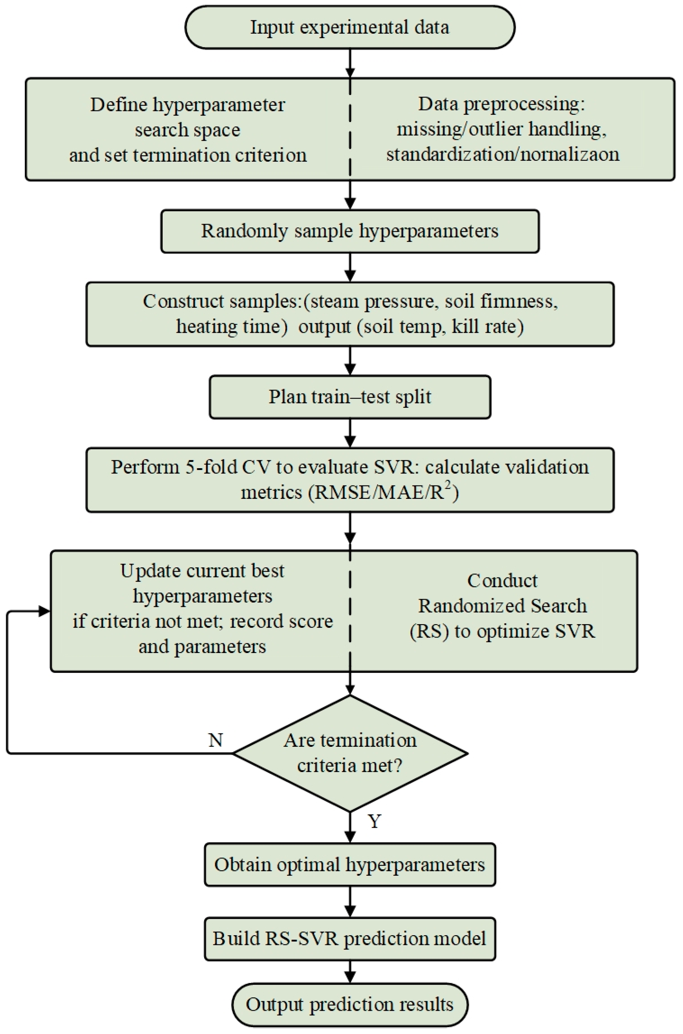
Hyperparameter tuning was first performed within the cross-validation framework to identify the best configuration for each model. Final model performance was then estimated using 100 repetitions of 5-fold cross-validation with random shuffling, so that the reported predictive accuracy reflected repeated validation rather than a single split. Early stopping was incorporated for MLP to prevent overfitting. Using the RS-SVR model as an example, the hyperparameter-optimization and validation workflow is illustrated in Figure 2 [31,32].
After preprocessing and standardization, candidate hyperparameter combinations were evaluated using 5-fold cross-validation. Final model performance was then assessed using 100 repetitions of 5-fold cross-validation with R2, MAE, and RMSE.

2.5. Energy-Cost Analysis and Efficiency Evaluation

In practical applications, two operational variables are often predetermined, and the third control factor must be optimized to achieve the best overall performance. To evaluate the economic implications of different parameter combinations, we developed models for energy consumption and operating cost.

2.5.1. Energy Consumption of Steam Disinfestation

Energy consumption was calculated by considering the following components:
(1) Baseline energy consumption
Ebase is primarily determined by Pboiler and theat. Assuming Pboiler =15 kW and theat (min), the baseline energy is computed as in Equation (17).
E b a s e = P b o i l e r × t h e a t 60  
(2) Pressure-related energy consumption
Higher Psteam requires additional energy to maintain the operating pressure. This pressure-dependent consumption is adjusted using a pressure factor, as shown in Equation (18).
f p r e s s u r e = 1 + 0.1 × P
where P denotes Psteam (Mpa). The coefficient 0.1 indicates that Ebase increases by 1% for every 0.1 Mpa increase in pressure.
(3) The Etotal is computed using Equation (19).
E t o t a l = E b a s e × f p r e s s u r e = 15 × T 60 × ( 1 + 0.1 × P )
It is important to note that the energy-consumption model presented above is a simplified engineering approximation. The linear relationships in Equations (16)–(18) assume steady-state operation and do not account for thermal losses during steam transmission, warm-up transients, variations in boiler efficiency with pressure, or environmental factors such as ambient temperature and soil moisture content. These simplifications were adopted due to the lack of real-time power monitoring in the current experimental setup. Nevertheless, the model provides a reasonable first-order estimate for comparative optimization under controlled conditions. Future work should incorporate direct measurements of instantaneous power consumption to validate and refine the model, potentially using data-driven approaches to capture nonlinear dynamics.

2.5.2. Operating Cost

Operating cost was calculated from Etotal and the electricity tariff.
Based on the current industrial pelectricity, the tariff was set to pelectricity = 0.11$ kWh−1 (Equation (20)).
C e l e c t r i c i t y = E t o t a l × p e l e c t r i c i t y = E t o t a l × 0.11
Total cost is proportional to Etotal; therefore, reducing energy use through parameter optimization directly lowers operating cost.

2.5.3. Energy Utilization Efficiency

To jointly evaluate disinfestation performance and energy use, an efficiency metric was defined (Equation (21)).
F e n e r g y = K i l l R a t e E t o t a l
This metric represents the kill rate achieved per unit of Etotal; larger values indicate higher energy utilization efficiency. It integrates efficacy and energy-cost considerations and enables comprehensive comparison across candidate schemes.

2.6. Intelligent Decision Design

Three optimization modes were designed to meet practical requirements [33]:

2.6.1. Kill-Rate Maximization Mode (Optimized-High)

This mode targets scenarios where disinfestation efficacy is paramount. Under the constraint of a minimum-kill-rate requirement (≥95%), the system maximizes the kill rate to ensure complete pathogen inactivation. This mode may sacrifice energy efficiency to some extent.

2.6.2. Energy Minimization Mode (Optimized-Energy)

This mode is intended for cost-sensitive applications. While satisfying the kill-rate constraint, the system minimizes energy consumption and operating cost, thereby improving economic performance and maximizing energy savings without compromising efficacy.

2.6.3. Efficiency Maximization Mode (Optimized-Optimal)

This mode addresses scenarios requiring a balance between efficacy and cost. By jointly considering kill rate and energy consumption, it selects the solution that maximizes the efficiency metric (kill rate/energy), achieving an optimal trade-off between performance and cost.

2.6.4. Constrained Search and Decision Workflow

The proposed decision strategy was implemented through a grid-search approach. In brief, (i) fixed parameters were specified according to the application scenario (e.g., Pboiler and pelectricity), and the decision variable to be optimized was identified (e.g., theat); (ii) a search space was defined based on the physically feasible domain of the decision variable (e.g., setting theat to 5–15 min and generating 20 evenly spaced candidates); (iii) the trained predictive models were used to evaluate each candidate with respect to multiple metrics, including Tsoil, Killrate, Etotal, operating cost, and the composite efficiency index; (iv) feasible solutions were filtered by constraints (primarily Killrate ≥ 95%); (v) the optimal solution was selected from the feasible set according to the target objective (maximize kill rate, minimize energy, or maximize efficiency); and (vi) the recommended parameters and their corresponding predicted performance and cost metrics were reported, accompanied by visualizations illustrating how the decision variable influences each metric. The constrained search and decision workflow is summarized in Algorithm 1.
Algorithm 1. Multi-Model Prediction and Constrained Decision (Grid Search).
Input:
  • Dataset D = {(Psteam,i, Csoil,i, theat,i) → (Tsoil,i, Killrate,i)}i = 1…N
  • Model set M = {RF, SVR, MLP};
  • Hyperparameter tuning by RS + 5-fold CV
  • Final validation by 100 repetitions of 5-fold CV
  • Minimum kill-rate threshold: τkill = 95%
  • Pboiler = 15 kW; pelectricity = 0.11 $ kWh−1
  • Fixed setting S (two fixed parameters among {Psteam, Csoil, theat} with given values)
  • Decision variable v ∈ {Psteam, Csoil, theat}; search grid V = {vmin, vmin + Δv,…, vmax}
  • Mode ∈ {Optimized-High, Optimized-Energy, Optimized-Optimal}
Output:
Recommended parameters θ* = (Psteam, *, Csoil, *, theat, *)
Predicted metrics: T ^ s o i l , , K ^ i l l l ( r a t e , i ) , Etotal, *, Celectricity *, Efficiency *
  • Standardize (Psteam, Csoil, theat) and split D into train/test
  • Tune each mM by RS + 5-fold CV; select best fT and fK by highest CV R2
  • BestScore ← −∞; BestSolution ← NULL
  • for each vi in V do
  • Construct candidate θi = Psteam, i, Csoil, i, theat, i using fixed setting S and vi
  • T ^ s o i l , i fT(Psteam, i, Csoil, i, theat, i)
  • K ^ i l l ( r a t e , i ) fK(Psteam, i, Csoil, i, theat, i); clip to [0, 100]
  • Ebase, iPboiler × theat, i/60
  • kpress, i ← 1 + 0.01 × ((Psteam, i − 0.1)/0.1)
  • Etotal, iEbase, i × kpress, i
  • Costtotal, ipelectricity × Etotal, i
  • Efficiencyi K ^ i l l ( r a t e , i ) /Etotal, i
  • if K ^ i l l ( r a t e , i ) τkill then
  • Scorei ← ComputeScore(mode, K ^ i l l ( r a t e , i ) , Etotal, i, Efficiencyi)
  • if Scorei > BestScore then update BestSolution with(θi, T ^ s o i l ,   i ,   K ^ i l l ( r a t e , i ) , Etotal, i, Costtotal, i, Efficiencyi)
  • end if
  • end for
  • if BestSolution == NULL then BestSolution K ^ i l l ( r a t e , i )
  • return BestSolution
  • arg max v i V K ^ i l l r a t e , i
  • Function ComputeScoremode, K ^ i l l ( r a t e ) , Etotal, Efficiency:
  • if mode == Optimized-High:
  • return K ^ i l l ( r a t e )
  • if mode == Optimized-Energy:
  • return Etotal
  • if mode == Optimized-Optimal:
  • return Efficiency
The time complexity of the algorithm is O(n), where n is the size of the search grid (typically 20 candidates). The method is simple and efficient, enabling rapid identification of an optimal solution that satisfies the imposed constraints.

3. Results

3.1. Effects of Key Variables on Disinfestation Performance

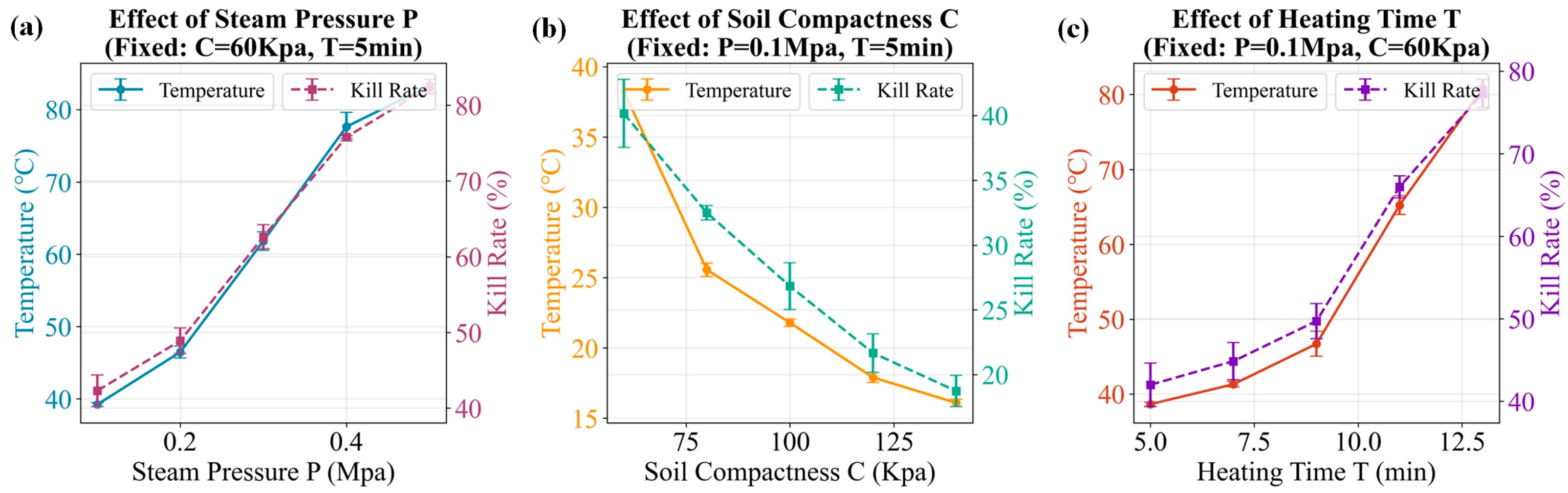
To better understand how Psteam, Csoil, and theat affect disinfestation outcomes, we first performed a systematic analysis of the experimental data. Figure 3 summarizes the single-factor response trends of the input variables on Tsoil and root-rot Killrate.
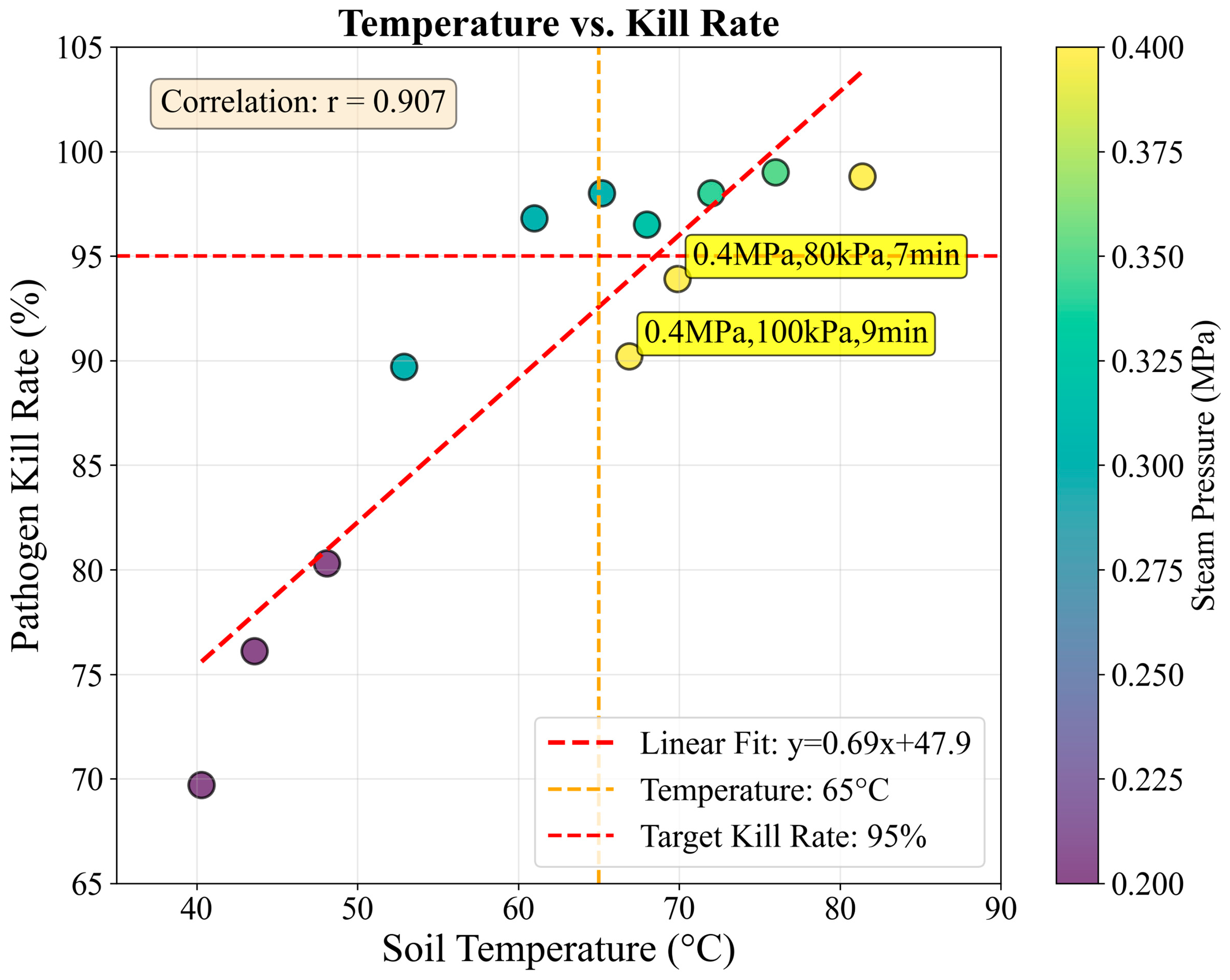
As shown in Figure 3, (1) Psteam is positively associated with both temperature and kill rate; however, the marginal gains diminish as pressure increases, indicating pronounced nonlinearity. (2) Csoil is negatively correlated with both responses. Higher compaction reduces pore space and increases resistance to steam penetration and heat conduction, resulting in more heterogeneous heating and reduced disinfestation efficacy. (3) theat is also positively related to temperature and kill rate. Notably, during the late heating stage (theat > 9 min), both warming and inactivation rates increase markedly, suggesting a cumulative heat effect that is informative for determining a cost-effective heating duration. Figure 4 further reveals the intrinsic relationship between Tsoil and kill rate.
A strong positive correlation was observed between soil temperature and pathogen kill rate (r = 0.907). For the vast majority of data points, when Tsoil exceeded 65 °C, the Killrate reached above 95%, meeting the basic requirement for agricultural disinfestation. However, two points in the 65–70 °C range (0.4 MPa, 80 kPa, 7 min → 69.9 °C, 93.9%; 0.4 MPa, 100 kPa, 9 min → 66.9 °C, 90.2%) exhibited lower kill rates. Analysis indicates that these exceptions result from insufficient heating duration (≤9 min) and/or high soil compaction (≥80 kPa), which lead to inadequate thermal dose and heterogeneous steam penetration. Therefore, in practice, to reliably achieve Killrate ≥ 95%, it is recommended to control the target temperature above 70 °C, with heating time ≥ 9 min and soil compaction ≤ 80 kPa. This finding supports the subsequent strategy of using temperature as a key control indicator while recognizing the need to consider heating time and soil conditions in predictive modeling. To examine multiparameter interactions, Figure 5 presents heat maps showing how combinations of the other two parameters shape the soil-temperature distribution when one parameter is fixed.
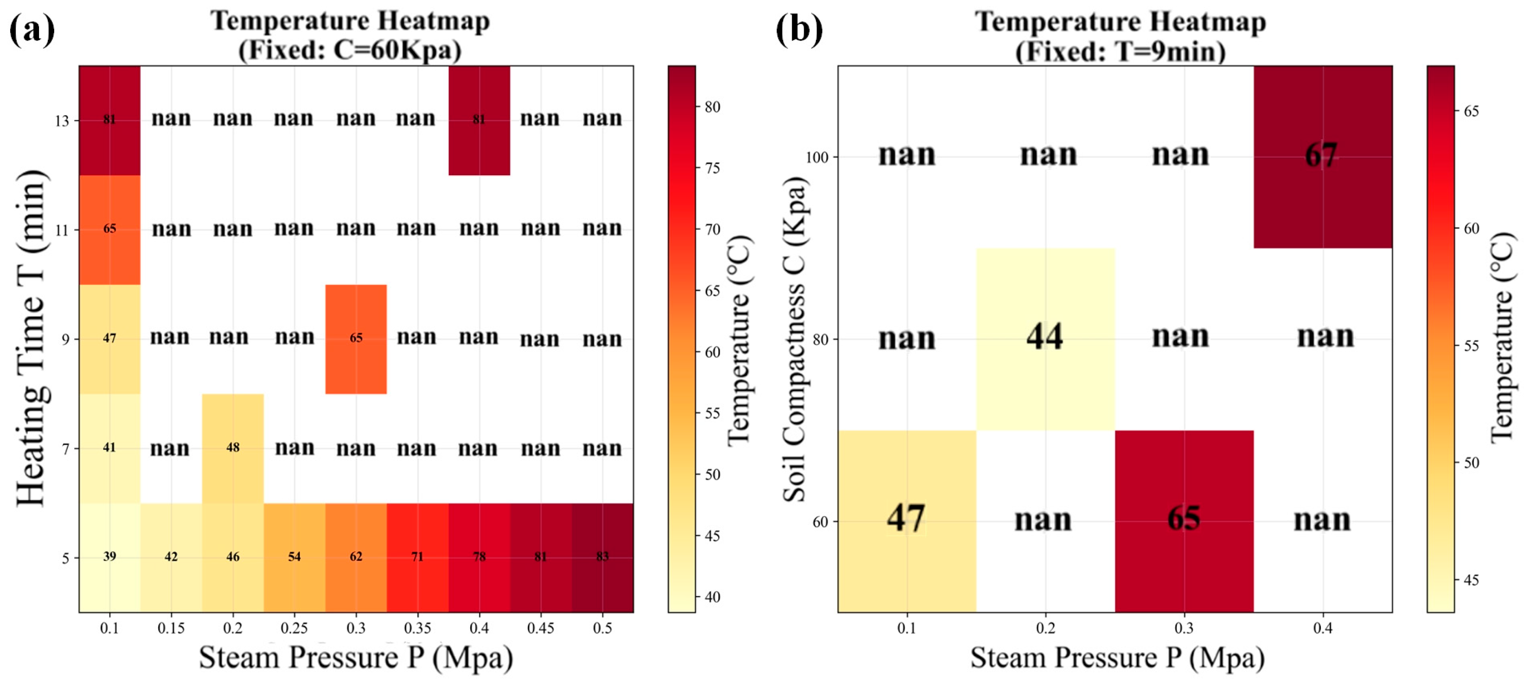
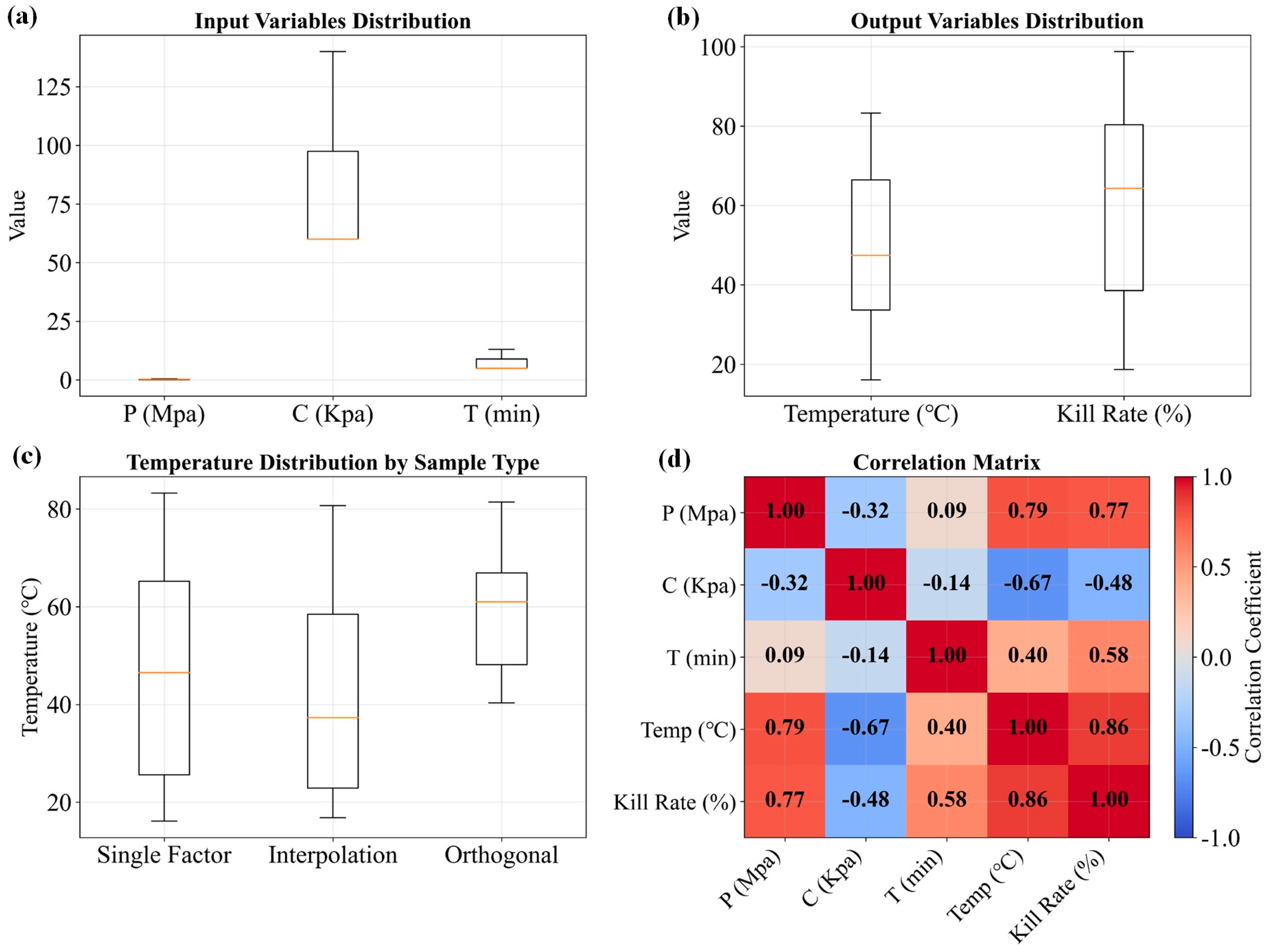
As shown in Figure 5a, with Csoil fixed at 60 kPa, high-temperature regions cluster in the “high-pressure–long-time” combinations. In Figure 5b, when theat is fixed at 9 min, higher compaction markedly suppresses temperature elevation. These results indicate that Psteam, Csoil, and theat must be coordinated in practice to avoid locally insufficient temperatures and potential “blind spots” in disinfestation caused by improper single-parameter settings. Figure 6 provides an overview of the distributions and correlation structure of all variables.
All input and output variables fell within reasonable ranges without anomalous distributions. The strong correlation between temperature and kill rate further supports the feasibility of indirectly assessing disinfestation efficacy via temperature prediction. In addition, correlations among the input variables were weak, suggesting that the experimental design effectively mitigated multicollinearity, which benefits model construction and interpretation.

3.2. Predictive Performance of Different Regression Models

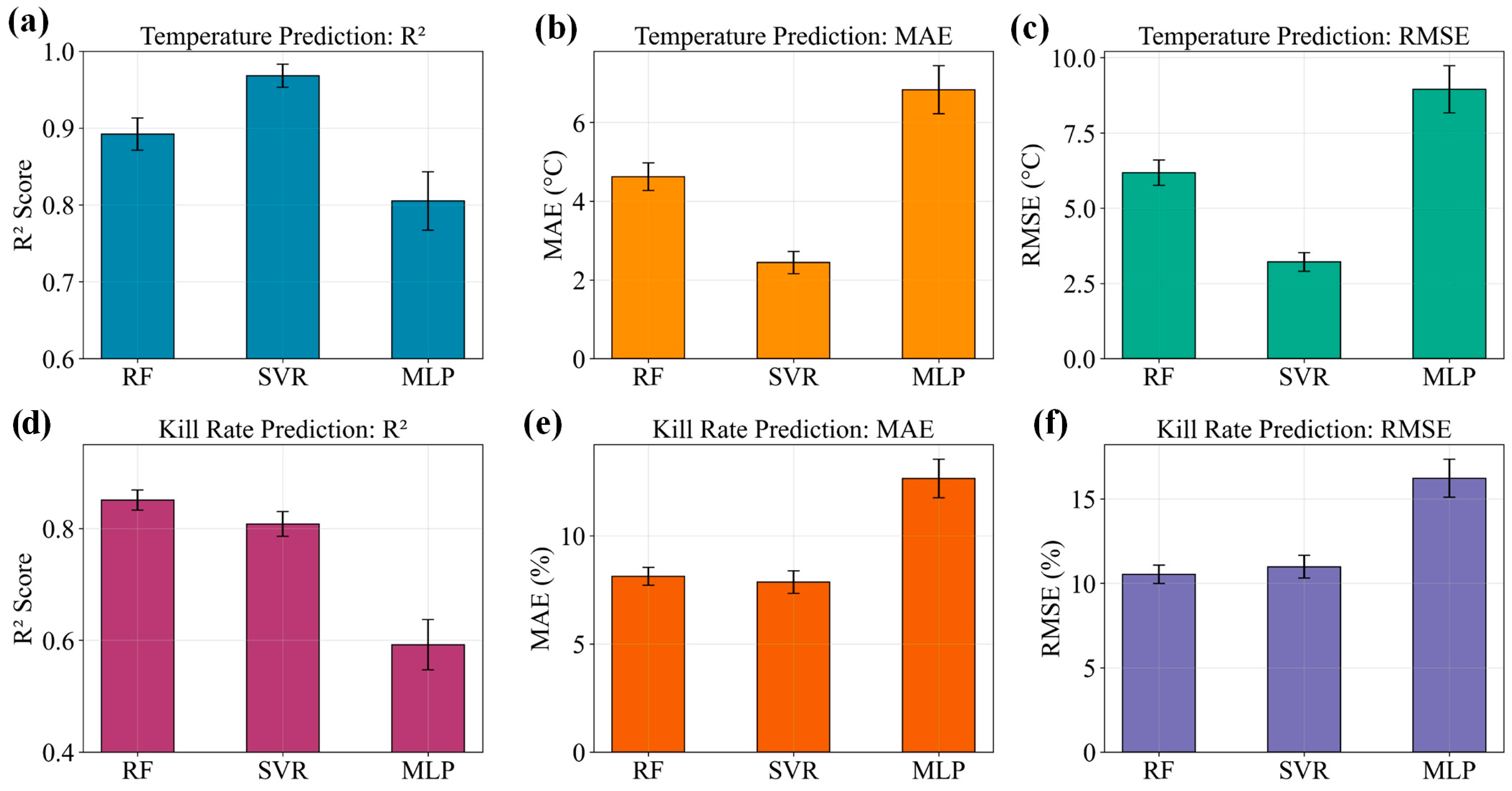
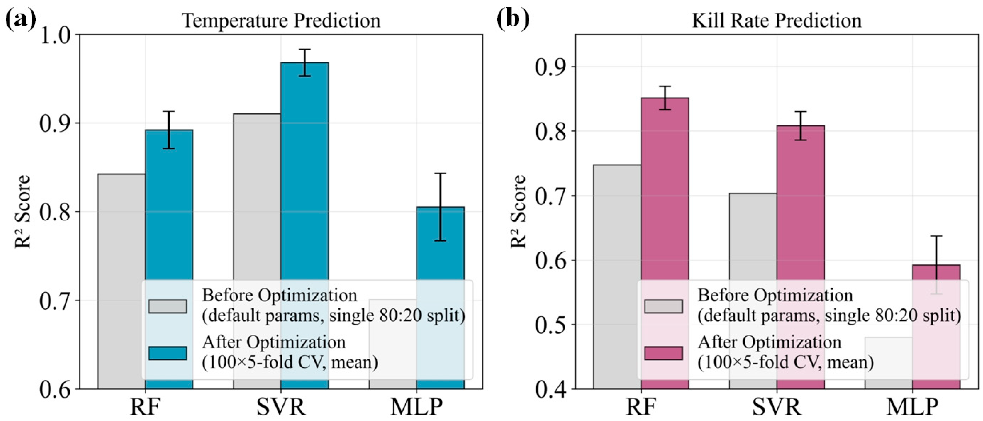
To evaluate the predictive capability of different machine learning algorithms for soil steam disinfestation, we systematically compared RF, SVR, and MLP before and after hyperparameter optimization using random search (RS). The dataset comprised 72 valid samples (45 from single-factor experiments and 27 from the L9(33) orthogonal design). To ensure robust and statistically reliable evaluation, we performed 100 repetitions of 5-fold cross-validation with random shuffling. Model performance was measured using the coefficient of determination (R2), mean absolute error (MAE), and root mean squared error (RMSE). All metrics are reported as mean ± 95% confidence interval (CI) over the 100 repetitions. The Friedman test with post hoc Nemenyi correction was used to compare model performance statistically. Table 3 summarizes the performance of the three optimized models. For Tsoil prediction, SVR achieved the highest R2 (0.968 ± 0.015), lowest MAE (2.44 ± 0.28 °C), and lowest RMSE (3.21 ± 0.31 °C), significantly outperforming RF (R2 = 0.892 ± 0.021, MAE = 4.62 ± 0.35 °C, RMSE = 6.18 ± 0.42 °C) and MLP (R2 = 0.805 ± 0.038, MAE = 6.83 ± 0.61 °C, RMSE = 8.95 ± 0.78 °C). For Killrate prediction, RF yielded the highest R2 (0.851 ± 0.018) and lowest RMSE (10.53 ± 0.55%), while SVR showed slightly lower but still acceptable performance (R2 = 0.808 ± 0.022, RMSE = 10.98 ± 0.67%). MLP performed poorly for kill-rate prediction (R2 = 0.592 ± 0.045, RMSE = 16.23 ± 1.12%).
The Friedman test indicated significant differences between the three models for both prediction tasks (p < 0.01). Post hoc Nemenyi test confirmed that SVR significantly outperformed RF and MLP for Tsoil prediction (p < 0.05). For Killrate prediction, RF outperformed MLP significantly (p < 0.05), but the difference between RF and SVR was not statistically significant (p = 0.08). Figure 7-presents a visual comparison of the three models.
Figure 8 displays the predicted versus observed values for the selected RS-SVR model based on cross-validation predictions.
Based on these results, RS-SVR was selected as the core predictor in our multi-output regression framework for the following reasons:
Priority of temperature prediction: Tsoil is a core variable that can be directly monitored during steam disinfestation and has clear physical interpretability. As shown in Figure 4, temperature is strongly and positively correlated with kill rate (r = 0.907), and when Tsoil exceeds 65 °C under proper heating duration (≥9 min) and moderate compaction (≤80 kPa), Killrate consistently reaches ≥95%. Therefore, accurate temperature prediction is fundamental to ensuring disinfestation efficacy.
Consistency for dual-output prediction: SVR substantially outperformed RF in temperature prediction (ΔR2 = +0.076, MAE reduction of 2.18 °C). Although its kill-rate R2 was slightly lower than that of RF, the difference was not statistically significant (p = 0.08). Moreover, the predicted kill-rate trends from SVR remained highly coherent with temperature, aligning better with the underlying physical principle that higher temperatures lead to higher inactivation.
Robustness and generalization: The structural risk minimization principle of SVMs often yields stronger generalization under small-sample conditions. The cross-validation results showed that SVR performed more consistently across data subsets (narrower confidence intervals for temperature prediction), which is important given potential parameter fluctuations in real production settings.
In summary, RS-SVR provided the best balance of temperature accuracy, inter-output consistency, and system robustness, and was therefore selected as the core predictor.

3.3. Intelligent Decision-Making in Representative Scenarios

Building on the optimal predictor (RS-SVR), we implemented an intelligent decision system for soil steam disinfestation in P. notoginseng cultivation. Given user-specified fixed parameters and an optimization objective, the system automatically recommends the optimal value of the third parameter to dynamically balance disinfestation efficacy, energy use, and operating cost. The effectiveness and practicality of the strategy were validated through system tests in three representative scenarios. All scenarios enforced a baseline constraint of Killrate ≥ 95% to ensure compliant disinfestation performance.

3.3.1. Time-Domain Optimization: Dynamic Adjustment of Heating Duration

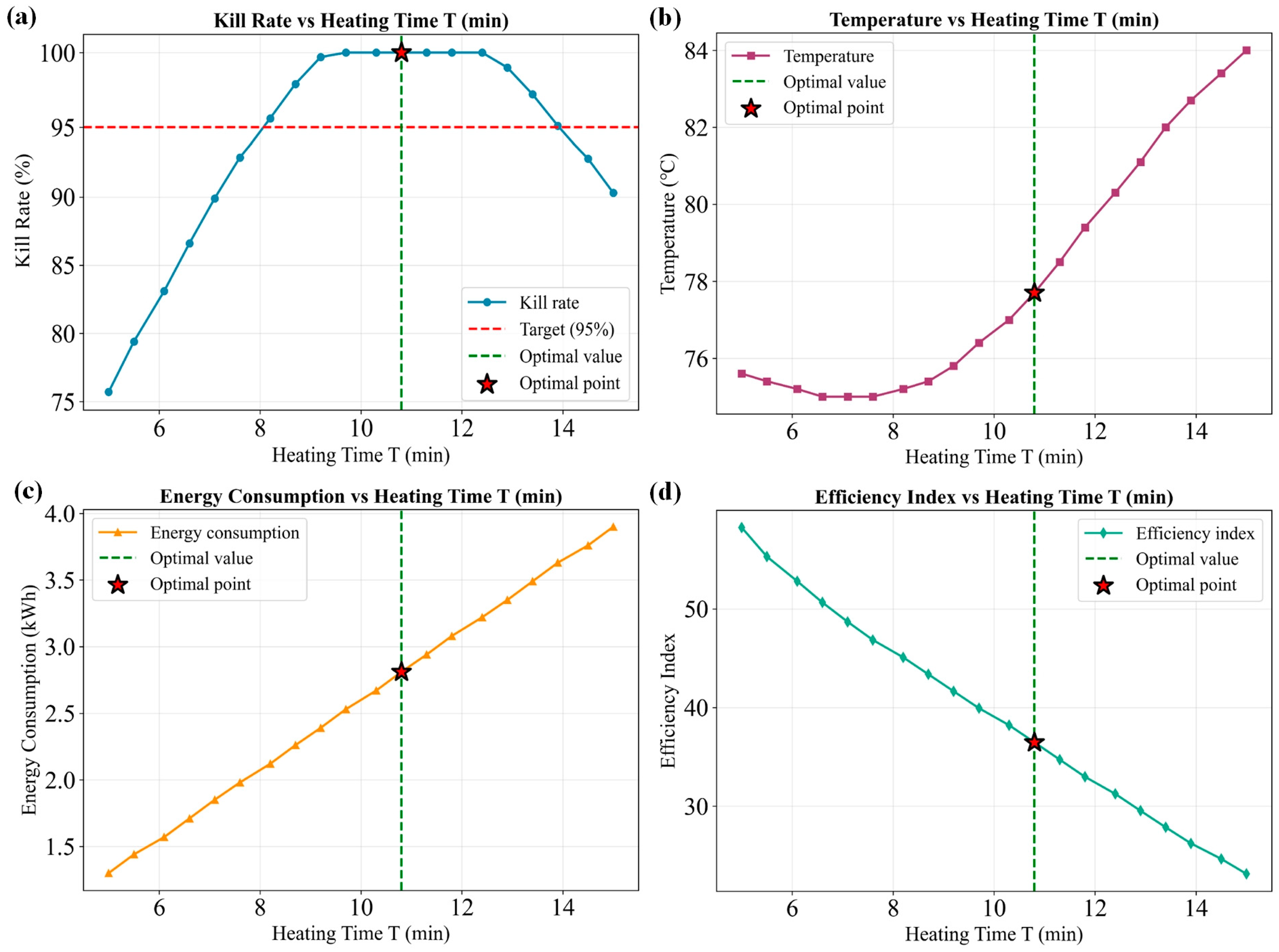
In practice, Psteam and Csoil are often constrained by equipment capability and field conditions, making theat the primary adjustable variable. In this scenario, Psteam was fixed at 0.4 MPa and Csoil at 60 kPa. With the objective of “maximizing kill rate,” theat was optimized over the range of 7–13 min.
As theat increased, both Tsoil and kill rate rose gradually, whereas energy consumption increased approximately linearly. The system recommended an optimal theat of 10.8 min, yielding a predicted Tsoil of 77.7 °C and a kill rate of 100% (the raw model output was 102.3%, which was clipped to the practical maximum of 100% as implemented in Algorithm 1), with an Etotal of 2.81 kWh and a cost of 0.32 $ (Figure 9). Compared with the empirical setting of theat = 13 min, this solution reduced energy use by ~13.5% while maintaining the required kill rate, demonstrating the system’s energy-saving capability through time-domain regulation.

3.3.2. Media Adaptation: Recommendations for Soil-Compaction Regulation

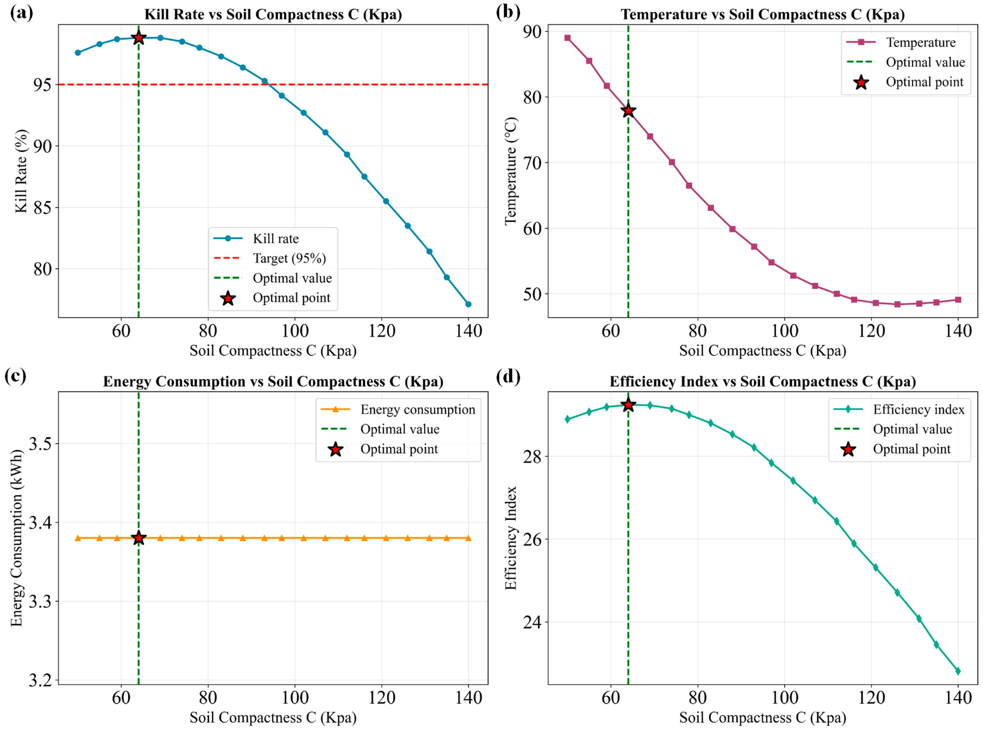
Csoil can be adjusted in practice through tillage operations. In this scenario, Psteam was fixed at 0.4 MPa and theat at 13 min. With the objective of “maximizing efficiency,” Csoil was searched over 60–100 kPa.
As Csoil increased, steam penetration decreased, leading to pronounced reductions in Tsoil and kill rate. The system recommended an optimal Csoil of 64.0 kPa, corresponding to a predicted temperature of 77.9 °C, a kill rate of 98.8%, energy consumption of 3.38 kWh, and a cost of 0.39$ (Figure 10). If the initial compaction is too high (e.g., Csoil > 90 kPa), the system flags the need for loosening measures (e.g., tillage); otherwise, the kill-rate constraint cannot be satisfied under the specified Psteam and theat. This result indicates that the system can provide not only optimal parameter values but also actionable recommendations for field operations.

3.3.3. Power-Parameter Optimization: Energy-Saving Steam-Pressure Setting

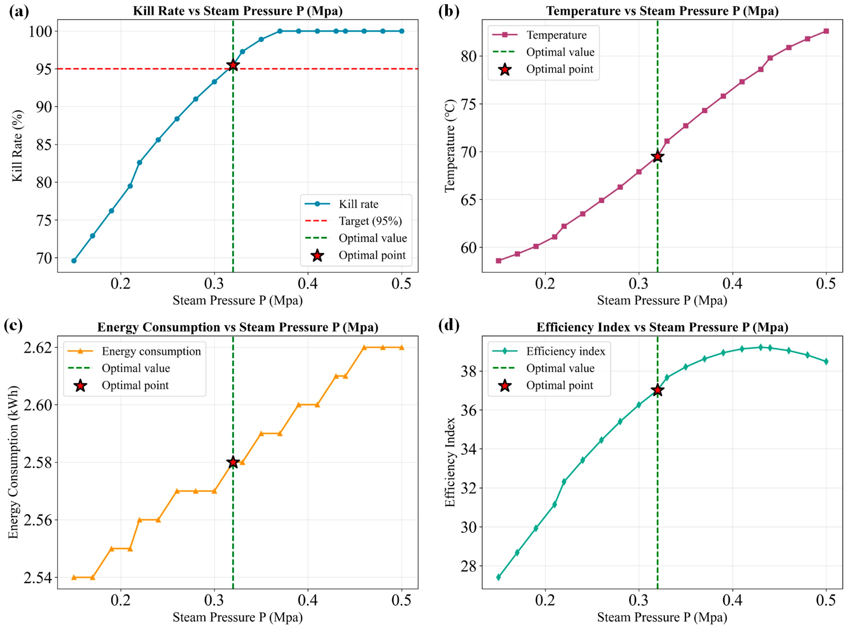
Within the allowable operating range, Psteam is a key factor governing disinfestation rate and energy consumption. In this scenario, Csoil was fixed at 60 kPa and theat at 10 min. With the objective of “minimizing energy consumption,” Psteam was optimized over 0.2–0.5 MPa.
The system recommended an optimal Psteam of 0.32 MPa, yielding a predicted temperature of 69.5 °C, a kill rate of 95.5%, energy consumption of 2.58 kWh, and a cost of 0.30$ (Figure 11). Compared with a commonly used high-pressure setting (e.g., 0.5 MPa), this solution reduced energy use by 18.2% while maintaining Killrate above 95%. This demonstrates that, while meeting disinfestation requirements, appropriately lowering Psteam can substantially reduce energy consumption, which is particularly valuable in cost-sensitive production scenarios.

3.4. Benefit Comparison Between Intelligent Decision-Making and Empirical Tuning

To comprehensively evaluate the practical benefits of the proposed intelligent optimization strategy, we conducted a systematic comparison between conventional experience-based tuning and the model-driven decision approach. The conventional method followed a fixed parameter set commonly used in local practice (typically higher pressure and longer theat to ensure efficacy; e.g., Psteam = 0.45 MPa, Csoil = 80 kPa, theat = 12 min). The optimized method used the recommended parameter sets generated by the intelligent decision system under the scenarios in Section 3.3, and their average performance was used for comparison. Comparisons were conducted along three core dimensions—energy consumption, operating cost, and disinfestation efficacy—and their practical applicability was discussed.
The optimized approach achieved an average energy consumption of 2.94 kWh, compared with 3.46 kWh for the conventional approach, corresponding to a 14.9% reduction. This improvement primarily stems from the system’s ability to use model-based predictions to reduce unnecessary theat or Psteam while maintaining the kill-rate constraint, thereby avoiding wasted energy. In particular, under the “minimize energy” mode, the system preferentially selects pressure–time combinations with higher energy efficiency, leading to markedly lower overall electricity use.
Using the industrial electricity tariff 0.11 $ kWh−1, the optimized method reduced the average cost per disinfestation cycle to 0.34 $, compared with 0.40 $ for the conventional method, i.e., a 14.9% saving. The cost reduction mirrored the decrease in energy use, indicating that economic benefits were achieved directly through energy savings. If deployed in large-scale production (e.g., 10 disinfestation cycles per season per 100 mu of cultivated area), the projected savings could reach several thousand USD per production cycle, indicating strong economic potential for adoption.
Despite clear advantages in energy and cost, the optimized method did not compromise disinfestation efficacy. All optimized solutions satisfied the baseline constraint of Killrate ≥ 95%, and in some scenarios, the kill rate approached complete inactivation (>98%). This confirms that the system does not simply trade efficacy for energy savings; rather, it leverages accurate prediction to locate an optimal balance between efficacy and energy input.
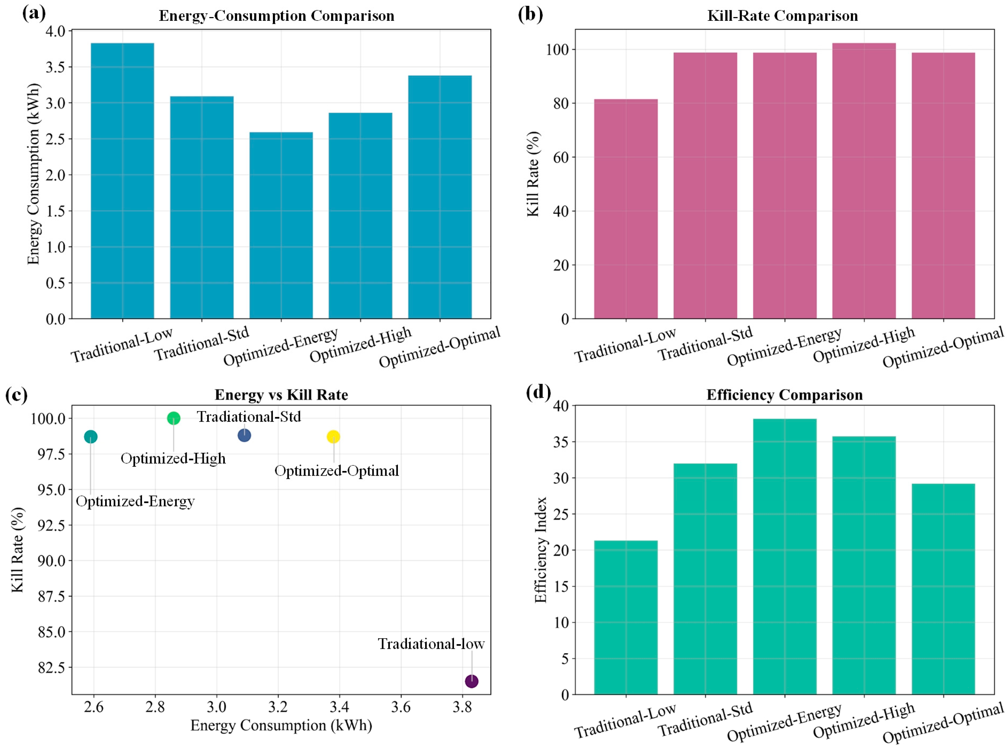
In summary, the intelligent decision-based control strategy matches conventional practice in disinfestation efficacy while delivering substantial gains in energy efficiency and cost effectiveness, supporting its practical value and scalability. Figure 12 summarizes comparisons across the different control strategies.

4. Discussion

This study established a multi-output regression framework coupled with a multi-mode intelligent decision system to address the core challenge in soil steam disinfestation for P. notoginseng: reconciling the inherent trade-off between disinfection efficacy and energy consumption. The results demonstrate that the proposed approach not only achieves high-fidelity prediction of treatment outcomes but also enables scenario-adaptive optimization, offering a significant advancement over conventional empirical operation.
The superior performance of the RS-optimized SVR model (Tsoil R2 = 0.968, MAE = 2.44 °C; Killrate R2 = 0.808) underscores the importance of incorporating physical coupling mechanisms into predictive modeling. By treating Tsoil and Killrate as jointly predicted variables rather than independent targets, the multi-output framework implicitly leverages the Arrhenius-type thermal death kinetics [16,17], where kill rate is a time-integral function of temperature. This approach aligns with recent advances in multi-target regression for agricultural applications [22,25] and addresses the generalization limitations often encountered under small-sample conditions [18]. Although RF yielded a marginally higher R2 for kill-rate prediction alone, the SVR model’s structural risk minimization principle provides superior robustness and inter-output consistency—a critical advantage when predictions inform downstream decision-making. The strong positive correlation between Tsoil and Killrate (r > 0.90) and the identification of 65 °C as a reliable surrogate threshold further validate the physical interpretability of the modeling framework, providing a straightforward control reference for practical operation.
The developed multi-mode decision algorithm departs from the conventional single-objective optimization approaches commonly used in soil disinfestation research [4,19,20]. By integrating energy-consumption analysis (Etotal, Celectricity) with efficacy constraints, the system enables flexible adaptation to diverse production scenarios. The three tailored modes—maximizing kill rate, minimizing energy consumption, and maximizing efficiency—address distinct operational priorities that previous studies have treated as mutually exclusive. For instance, while Fennimore et al. [4] and Gay et al. [19] demonstrated the energy-saving potential of steam optimization, their frameworks lacked the flexibility to prioritize efficacy under high-risk disease pressure or to balance multiple objectives simultaneously. The constrained grid-search implementation (Algorithm 1) provides a computationally efficient and interpretable decision mechanism, with a time complexity of O(n), in contrast to “black-box” optimization methods that may obscure the rationale behind parameter recommendations [33]. The practical validation across three representative scenarios reveals substantial operational benefits. In the time-domain optimization (Section 3.3.1), dynamic adjustment of theat reduced energy consumption by ~13.5% compared to fixed-duration empirical settings while maintaining kill-rate compliance. This finding directly addresses the “disinfection blind spots” problem identified in static one-factor experiments [3], where inadequate heating duration under suboptimal pressure–compaction combinations can leave pathogen refugia. The media-adaptation scenario (Section 3.3.2) demonstrates the system’s capacity to translate predictive insights into actionable field recommendations: when Csoil exceeds 90 kPa under fixed Psteam and theat, the algorithm flags the need for tillage intervention—a decision rule that integrates physical understanding of steam penetration limitations [1,3] with real-time predictive capability. Most notably, the power-parameter optimization (Section 3.3.3) achieved an 18.2% reduction in operating cost while satisfying Killrate ≥ 95%, illustrating that significant energy savings are attainable without compromising efficacy when optimization is guided by accurate predictive models rather than heuristic safety margins.
The aggregate benefit analysis (Section 3.4) quantifies the system’s value proposition: 14.9% reductions in both energy consumption and operating cost relative to conventional practice, with projected seasonal savings reaching several thousand USD per 100 mu of cultivated area. These figures are particularly significant given the rising energy costs in protected agriculture [5,6] and the economic pressures facing continuous-cropping systems [18]. Importantly, the optimized solutions did not trade efficacy for efficiency—all recommendations satisfied the ≥95% kill-rate constraint, and in several scenarios achieved near-complete inactivation (>98%). This outcome suggests that conventional empirical operation, while ostensibly “safe” due to conservative high-input settings, may actually incur substantial energy waste without proportional gains in disinfestation certainty.
The proposed framework also contributes to the broader discourse on machine learning applications in agriculture. While previous reviews [10,15] have documented extensive use of RF, SVR, and MLP for yield prediction and environmental monitoring, their application to soil disinfestation parameter optimization has been limited. The systematic benchmarking with RS hyperparameter tuning (Section 2.4) provides a reproducible methodology for model selection in similar small-sample agricultural engineering contexts. Moreover, the integration of predictive modeling with explicit decision logic addresses a common criticism of data-driven agricultural tools: that they generate predictions without actionable, context-aware recommendations [28]. By framing optimization as a constrained search problem with clearly defined modes, the system bridges the gap between algorithmic capability and practical usability.

4.1. Limitations

Nevertheless, several limitations of this study should be acknowledged. First, the experimental data were collected from a single soil type (typical red soil from Wenshan, Yunnan) with moisture content maintained within a fixed range (20 ± 1%). Soil texture and initial moisture content critically govern steam-driven heat and mass transfer in porous media [1,3]; therefore, the generalizability of the current model to other soil types (e.g., sandy or clay-rich soils) or extreme moisture conditions (drought or saturation) remains to be validated.
Second, the predictive models were trained on data from controlled experimental conditions (laboratory-scale steam unit, standardized soil preparation). Scaling to commercial field applications may introduce unmodeled dynamics, such as spatial heterogeneity in soil compaction or steam distribution, ambient temperature effects, and equipment variability [4,21].
Third, the current decision framework assumes that the user can specify fixed parameters and an optimization mode a priori. While this design simplifies implementation, it may not capture the full complexity of dynamic decision-making under uncertainty (e.g., weather variability, fluctuating electricity prices, or evolving disease pressure).
Fourth, the efficiency metric defined in this study (Killrate/Etotal) provides a useful composite index but does not account for time-dependent factors such as labor costs, equipment depreciation, or the opportunity cost of extended treatment durations. A more comprehensive life-cycle cost analysis [20] would be needed to capture these factors.
Another limitation is the absence of independent external validation using field-collected data from different sites or seasons. The current evaluation relied solely on repeated random splits of the 72-sample dataset. While 100 repetitions of 5-fold cross-validation provide internal robustness estimates, they do not guarantee generalizability to unseen operating conditions (e.g., different soil textures, moisture levels, or ambient temperatures). To partially mitigate this concern, we also performed leave-one-out cross-validation (LOOCV) as a more stringent test under small-sample conditions. The LOOCV results (mean R2 = 0.965 for Tsoil and 0.801 for Killrate) were consistent with the reported 5-fold CV results, suggesting that overfitting is not severe. Nonetheless, future studies should collect independent datasets from commercial production fields to validate model transferability.
Finally, while the RS-optimized SVR demonstrated strong performance, the modest improvement in kill-rate prediction after tuning (ΔR2 = +0.01) compared to MLP (ΔR2 = +0.1213) suggests that alternative architectures—such as deep neural networks with attention mechanisms [27] or gradient-boosting frameworks [17]—might further enhance predictive accuracy, particularly for the more challenging kill-rate task. Exploring ensemble methods that combine the strengths of multiple algorithms (e.g., SVR for temperature, gradient boosting for Killrate) within a unified multi-output structure could yield additional gains.

4.2. Future Perspectives

Future research should focus on several directions to extend the applicability and robustness of the proposed framework. First, cross-site validation across diverse pedoclimatic contexts is needed. Transfer learning or domain adaptation techniques [11] could reduce the need for extensive retraining when applying the system to new sites with different soil types or moisture regimes.
Second, field-scale validation trials should be conducted to assess the system’s performance under real production conditions. Integrating real-time sensor feedback (e.g., embedded thermocouples for closed-loop control) could enhance the system’s robustness and practical relevance by compensating for unmodeled dynamics such as spatial heterogeneity and ambient temperature effects.
Third, the decision framework could be extended to incorporate stochastic optimization or multi-objective evolutionary algorithms [33]. This would enable more sophisticated trade-off analyses, such as Pareto frontier generation to visualize the full spectrum of efficacy–cost compromises under uncertainty.
Fourth, a more comprehensive life-cycle cost analysis [20] could inform a richer set of optimization objectives tailored to specific production systems, accounting for labor, equipment depreciation, and other time-dependent factors beyond direct energy consumption.
Finally, exploring alternative machine learning architectures—including deep neural networks with attention mechanisms [27] and gradient-boosting frameworks [17]—as well as ensemble methods that combine multiple algorithms within a unified multi-output structure, could further improve predictive accuracy, especially for the more challenging kill-rate prediction task. Additionally, the framework should be extended to other crops and disinfestation methods (e.g., anaerobic soil disinfestation [1,6]) to maximize its impact.

5. Conclusions

1. A high-accuracy multi-output prediction model grounded in physical coupling was established. The SVR model optimized via RS performed best in capturing the nonlinear relationships between Psteam, Csoil, and theat and the resulting treatment outcomes, achieving an R2 of 0.968 for soil-temperature prediction and 0.808 for root-rot pathogen kill-rate prediction. The study further quantified a strong positive association between Tsoil and kill rate (correlation coefficient r > 0.85) and identified 65 °C as a reliable surrogate control threshold above which the kill rate remains stably greater than 95%, thereby providing a theoretical basis for data-driven precision regulation.
2. A multi-mode intelligent decision strategy balancing phytosanitary efficacy and energy efficiency was proposed. Under real-world operating constraints, the developed decision system can automatically optimize key operational variables and flexibly support three modes: maximizing kill rate, minimizing energy consumption, and maximizing efficiency. While meeting disease-control requirements, the intelligent optimization strategy reduced per-cycle energy consumption and operating cost by an average of 14.9% relative to conventional experience-based operation. This approach not only avoids energy waste caused by indiscriminate heating, but also offers an economically feasible intelligent solution to mitigate continuous-cropping constraints in P. notoginseng production.
Despite these advances in parameter optimization and intelligent decision-making, the training data were primarily collected from typical red soils in Wenshan, Yunnan Province, and the soil moisture content was maintained within a fixed range during experiments. Because soil texture and initial moisture content critically govern steam-driven heat and mass transfer, the generalizability of the current model to other soil types or extreme moisture conditions remains to be validated.

Author Contributions

Research conceptualization, L.J. and X.H.; methodology, L.J. and L.Y.; software, L.J. and L.Y.; validation, B.M. and L.Y.; formal analysis, L.J. and L.Y.; investigation, L.J., B.M., Y.Y. and H.Z.; resources, Y.Y.; data curation, L.J., B.M. and H.Z.; writing—original draft preparation, L.J.; writing—review and editing, Y.Y., H.Z. and X.H.; visualization, L.J. and B.M.; supervision, X.H.; project administration, X.H.; funding acquisition, X.H. All authors have read and agreed to the published version of the manuscript.

Funding

This research was funded by the National Natural Science Foundation of China, grant number 12562017, the Shaanxi Provincial Social Science Fund Project, grant number 2024P040, the Humanities and Social Sciences General Project of the Shaanxi Provincial Department of Education, grant number 24JK0259, and Young Talent Fund of Association for Science and Technology in Yanan, China.

Informed Consent Statement

Not applicable.

Data Availability Statement

The original contributions presented in this study are included in the article. Further inquiries can be directed to the corresponding author.

Acknowledgments

This work was supported by the Regional Science Fund of the National Natural Science Foundation of China (Grant No. 12562017), the Shaanxi Provincial Social Science Fund Project (Grant No. 2024P040), the Humanities and Social Sciences General Project of the Shaanxi Provincial Department of Education (Grant No. 24JK0259), and Young Talent Fund of Association for Science and Technology in Yanan, China.

Conflicts of Interest

The authors declare that they have no conflicts of interest.

Abbreviations

The following abbreviations are used in this manuscript:
PsteamSteam pressure
CsoilSoil compaction (penetration resistance)
theatHeating time
TsoilSoil temperature
KillratePathogen kill rate
PboilerRated boiler power
EbaseBaseline energy consumption
kpressPressure-related energy correction factor
EtotalTotal energy consumption per operation
pelectricityElectricity price
CelectricityElectricity cost per operation
EfficiencyEnergy-efficiency index (Killrate/Etotal)
DDataset, D = {(xiyi)} for i = 1…N
xiInput vector of sample i: {Psteam,i, Csoil,i, theat,i}
yiOutput vector of sample i: {Tsoil,i, Killratei}
NNumber of samples
fT(·)Regression model for Tsoil prediction
fK(·)Regression model for Killrate prediction
T ^ s o i l Predicted soil temperature
K ^ i l l r a t e Predicted kill rate
R2Coefficient of determination
MAEMean absolute error
RMSERoot mean squared error
MSEMean squared error (loss)
MNumber of trees in the forest
mtryNumber of features randomly selected at each split
G(m)Bootstrap resampled training subset m
hm(x) Prediction of tree m for input x
SSample set at a node
SL, SRLeft/right child-node sample sets
Var( )Variance
φ(·) Nonlinear feature mapping
wWeight vector
bBias term
CPenalty parameter
εε-insensitive tube radius
ξi, ξ i Slack variables for sample i
K(si, sj) Kernel function
γRBF kernel width
HNumber of hidden neurons (or hidden units)
αL2 regularization coefficient
ηLearning rate (if explicitly used)
ZT, ZKLoss for temperature/kill-rate tasks
τkillMinimum kill-rate threshold
SFixed setting (two fixed variables among {Psteam, Csoil, theat})
vDecision variable to be optimized
VSearch grid for v
vmin, vmaxLower/upper bounds of v
ΔvGrid step size
θiCandidate parameter set i
θ*Recommended optimal parameter set
ScoreiObjective score of candidate i
RFRandom forest
SVRSupport vector regression
MLPMultilayer perceptron
RSRandomized search
CVCross-validation
RBFRadial basis function

References

  1. Shrestha, U.; Ownley, B.H.; Littrell, J.J.; Rice, J.H.; Butler, D.M. Anaerobic Soil Disinfestation and Crop Rotation with Cover Crops Enhances Management of Black Root Rot in Strawberry Systems. Sci. Hortic. 2024, 337, 113504. [Google Scholar] [CrossRef] [Scilit]
  2. Liu, D.; Samtani, J.; Johnson, C.; Zhang, X.; Butler, D.M.; Derr, J. Brewer’s Spent Grain with Yeast Amendment Shows Potential for Anaerobic Soil Disinfestation of Weeds and Pythium Irregulare. Agronomy 2023, 13, 2081. [Google Scholar] [CrossRef] [Scilit]
  3. Candido, V.; D’Addabbo, T.; Miccolis, V.; Castronuovo, D. Weed Control and Yield Response of Soil Solarization with Different Plastic Films in Lettuce. Sci. Hortic. 2011, 130, 491–497. [Google Scholar] [CrossRef] [Scilit]
  4. Fennimore, S.A.; Martin, F.N.; Miller, T.C.; Broome, J.C.; Dorn, N.; Greene, I. Evaluation of a Mobile Steam Applicator for Soil Disinfestation in California Strawberry. HortScience 2014, 49, 1542–1549. [Google Scholar] [CrossRef] [Scilit]
  5. Gullino, M.L.; Garibaldi, A.; Gamliel, A.; Katan, J. Soil Disinfestation: From Soil Treatment to Soil and Plant Health. Plant Dis. 2022, 106, 1541–1554. [Google Scholar] [CrossRef] [Scilit] [PubMed]
  6. Guo, H.; Di Gioia, F.; Zhao, X.; Ozores-Hampton, M.; Swisher, M.E.; Hong, J.; Kokalis-Burelle, N.; DeLong, A.N.; Rosskopf, E.N. Optimizing Anaerobic Soil Disinfestation for Fresh Market Tomato Production: Nematode and Weed Control, Yield, and Fruit Quality. Sci. Hortic. 2017, 218, 105–116. [Google Scholar] [CrossRef] [Scilit]
  7. Michuda, A.; Goodhue, R.E.; Hoffmann, M.; Fennimore, S.A. Predicting Net Returns of Organic and Conventional Strawberry Following Soil Disinfestation with Steam or Steam Plus Additives. Agronomy 2021, 11, 149. [Google Scholar] [CrossRef] [Scilit]
  8. Sanabria-Velazquez, A.D.; Enciso-Maldonado, G.A.; Maidana-Ojeda, M.; Diaz-Najera, J.F.; Ayvar-Serna, S.; Thiessen, L.D.; Shew, H.D. Integrated Pathogen Management in Stevia Using Anaerobic Soil Disinfestation Combined with Different Fungicide Programs in USA, Mexico, and Paraguay. Agronomy 2023, 13, 1358. [Google Scholar] [CrossRef] [Scilit]
  9. Gilli, C.; Camps, C. Influence of Two Different Thermal Screen Managements on Yield, Quality and Energy Consumption of a Soilless Tomato Culture. Acta Hortic. 2012, 952, 97–102. [Google Scholar] [CrossRef] [Scilit]
  10. Liakos, K.G.; Busato, P.; Moshou, D.; Pearson, S.; Bochtis, D. Machine Learning in Agriculture: A Review. Sensors 2018, 18, 2674. [Google Scholar] [CrossRef] [Scilit]
  11. Abimbola, O.P.; Meyer, G.E.; Mittelstet, A.R.; Rudnick, D.R.; Franz, T.E. Knowledge-Guided Machine Learning for Improving Daily Soil Temperature Prediction across the United States. Vadose Zone J. 2021, 20, e20151. [Google Scholar] [CrossRef] [Scilit]
  12. de Carvalho Alves, M.; Sanches, L.; Pozza, E.A.; Pozza, A.A.A.; da Silva, F.M. The Role of Machine Learning on Arabica Coffee Crop Yield Based on Remote Sensing and Mineral Nutrition Monitoring. Biosyst. Eng. 2022, 221, 81–104. [Google Scholar] [CrossRef] [Scilit]
  13. Houben, T.; Ebeling, P.; Khurana, S.; Schmid, J.S.; Boog, J. Machine-Learning Based Spatiotemporal Prediction of Soil Moisture in a Grassland Hillslope. Vadose Zone J. 2018, 24, e70011. [Google Scholar] [CrossRef] [Scilit]
  14. Sunoj, S.; Yeh, B.; Marcaida, M., III; Longchamps, L.; van Aardt, J.; Ketterings, Q.M. Maize Grain and Silage Yield Prediction of Commercial Fields Using High-Resolution UAS Imagery. Biosyst. Eng. 2023, 235, 137–149. [Google Scholar] [CrossRef] [Scilit]
  15. Van Klompenburg, T.; Kassahun, A.; Catal, C. Crop Yield Prediction Using Machine Learning: A Systematic Literature Review. Comput. Electron. Agric. 2020, 177, 105709. [Google Scholar] [CrossRef] [Scilit]
  16. Carlesi, S.; Martelloni, L.; Bigongiali, F.; Frasconi, C.; Fontanelli, M.; Bàrberi, P. Effects of Band Steaming on Weed Control, Weed Community Diversity and Composition and Yield in Organic Carrot at Three Mediterranean Sites. Weed Res. 2021, 61, 385–395. [Google Scholar] [CrossRef] [Scilit]
  17. Huber, F.; Yushchenko, A.; Stratmann, B.; Steinhage, V. Extreme Gradient Boosting for Yield Estimation Compared with Deep Learning Approaches. Comput. Electron. Agric. 2022, 202, 107346. [Google Scholar] [CrossRef] [Scilit]
  18. Serrano-Pérez, P.; Rosskopf, E.; De Santiago, A.; Rodríguez-Molina, M.D.C. Anaerobic Soil Disinfestation Reduces Survival and Infectivity of Phytophthora nicotianae Chlamydospores in Pepper. Sci. Hortic. 2017, 215, 38–48. [Google Scholar] [CrossRef] [Scilit]
  19. Gay, P.; Piccarolo, P.; Aimonino, D.R.; Tortia, C. A High Efficiency Steam Soil Disinfestation System, Part I: Physical Background and Steam Supply Optimisation. Biosyst. Eng. 2010, 107, 74–85. [Google Scholar] [CrossRef] [Scilit]
  20. Raffaelli, M.; Martelloni, L.; Frasconi, C.; Fontanelli, M.; Carlesi, S.; Peruzzi, A. A Prototype Band-Steaming Machine: Design and Field Application. Biosyst. Eng. 2016, 144, 61–71. [Google Scholar] [CrossRef] [Scilit]
  21. Pan, S. Optimized Steam Boiler for Soil Steam Disinfection: Structural Design, CFD Simulation, and Field Application. PLoS ONE 2025, 20, e0340080. [Google Scholar] [CrossRef] [Scilit]
  22. Aguilar-Ariza, A.; Sotta, N.; Fujiwara, T.; Guo, W.; Kamiya, T. A Multi-Target Regression Method to Predict Element Concentrations in Tomato Leaves Using Hyperspectral Imaging. Plant Phenomics 2024, 6, 0146. [Google Scholar] [CrossRef] [Scilit]
  23. Melki, G.; Cano, A.; Kecman, V.; Ventura, S. Multi-Target Support Vector Regression via Correlation Regressor Chains. Inf. Sci. 2017, 415–416, 53–69. [Google Scholar] [CrossRef] [Scilit]
  24. Petersen, N.C.; Rodrigues, F.; Pereira, F.C. Multi-Output Bus Travel Time Prediction with Convolutional LSTM Neural Network. Expert Syst. Appl. 2019, 120, 426–435. [Google Scholar] [CrossRef] [Scilit]
  25. Santana, E.J.; Rodrigues dos Santos, F.; Mastelini, S.M.; Melquiades, F.L.; Barbon, S., Jr. Improved Prediction of Soil Properties with Multi-Target Stacked Generalisation on EDXRF Spectra. Chemom. Intell. Lab. Syst. 2021, 209, 104231. [Google Scholar] [CrossRef] [Scilit]
  26. Bayatvarkeshi, M.; Bhagat, S.K.; Mohammadi, K.; Kisi, O.; Farahani, M.; Hasani, A.; Deo, R.; Yaseen, Z.M. Modeling Soil Temperature Using Air Temperature Features in Diverse Climatic Conditions with Complementary Machine Learning Models. Comput. Electron. Agric. 2021, 185, 106158. [Google Scholar] [CrossRef] [Scilit]
  27. Li, X.; Zhang, L.; Wang, X.; Liang, B. Forecasting Greenhouse Air and Soil Temperatures: A Multi-Step Time Series Approach Employing Attention-Based LSTM Network. Comput. Electron. Agric. 2024, 217, 108602. [Google Scholar] [CrossRef] [Scilit]
  28. Kok, Z.H.; Mohamed Shariff, A.R.; Alfatni, M.S.M.; Khairunniza-Bejo, S. Support Vector Machine in Precision Agriculture: A Review. Comput. Electron. Agric. 2021, 191, 106546. [Google Scholar] [CrossRef] [Scilit]
  29. Rumelhart, D.E.; Hinton, G.E.; Williams, R.J. Learning Representations by Back-Propagating Errors. Nature 1986, 323, 533–536. [Google Scholar] [CrossRef] [Scilit]
  30. Yang, L.; Shami, A. On Hyperparameter Optimization of Machine Learning Algorithms: Theory and Practice. Neurocomputing 2020, 415, 295–316. [Google Scholar] [CrossRef] [Scilit]
  31. Miseta, T.; Fodor, A.; Vathy-Fogarassy, Á. Surpassing Early Stopping: A Novel Correlation-Based Stopping Criterion for Neural Networks. Neurocomputing 2024, 567, 127028. [Google Scholar] [CrossRef] [Scilit]
  32. Vilares Ferro, M.; Doval Mosquera, Y.; Ribadas Pena, F.J.; Darriba Bilbao, V.M. Early Stopping by Correlating Online Indicators in Neural Networks. Neural Netw. 2023, 159, 109–124. [Google Scholar] [CrossRef] [Scilit] [PubMed]
  33. Ponsich, A.; Domenech, B.; Ferrer-Martí, L.; Juanpera, M.; Pastor, R. A Multi-Objective Optimization Approach for the Design of Stand-Alone Electrification Systems Based on Renewable Energies. Expert Syst. Appl. 2022, 199, 116939. [Google Scholar] [CrossRef] [Scilit]
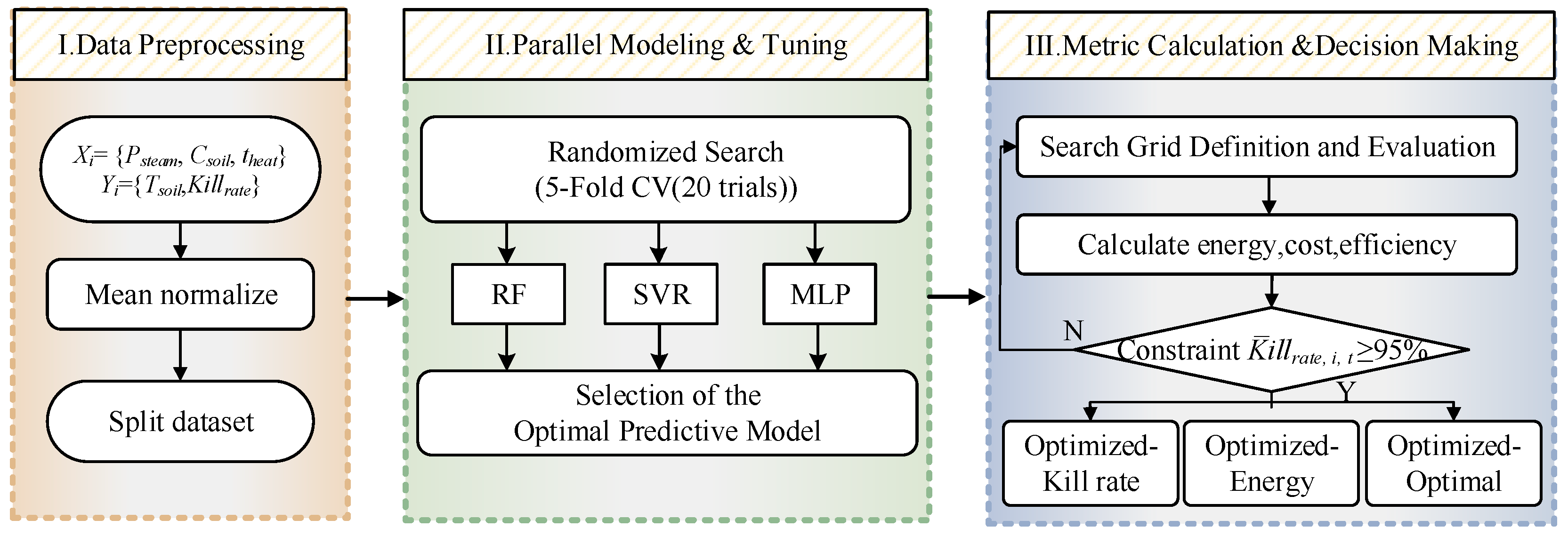
Figure 1. Overall technical route and research workflow. Arrows indicate the sequential flow of data and decision-making. The framework comprises (I) data preprocessing and train–test splitting, (II) RS-tuned multi-output regression (RF/SVR/MLP) for predicting Tsoil and Killrate, and (III) constrained grid search to optimize one operational variable under Killrate ≥ 95% with three modes (maximize Killrate, minimize energy/cost, or maximize efficiency).
Agronomy 16 00877 g001
Figure 2. Hyperparameter-optimization and validation workflow of the SVR model using randomized search (RS).
Agronomy 16 00877 g002
Figure 3. Single-factor response trends of Tsoil and Killrate during soil steam disinfestation. (ac) Line plots with error bars showing the effects of each input variable on Tsoil and Killrate. (a) Effect of Psteam (fixed: Csoil = 60 kPa, theat = 5 min). (b) Effect of Csoil (fixed: Psteam = 0.1 MPa, theat = 5 min). (c) Effect of theat (fixed: Psteam = 0.1 MPa, Csoil = 60 kPa). Error bars indicate variability across replicates.
Agronomy 16 00877 g003
Figure 4. Correlation analysis between Tsoil and Killrate (%) versus temperature (°C), colored by Psteam (MPa). Dashed line: linear fit (r = 0.907); vertical line: 65 °C threshold; horizontal line: 95% target. Two points in the 65–70 °C range (0.4 MPa, 80 kPa, 7 min → 69.9 °C, 93.9%; 0.4 MPa, 100 kPa, 9 min → 66.9 °C, 90.2%) fall below 95% due to insufficient heating time or excessive soil compaction.
Agronomy 16 00877 g004
Figure 5. Heat maps of soil-temperature distributions under multiparameter interactions. (a,b) Tsoil (℃) as a function of two-parameter combinations with one parameter fixed. (a) Csoil fixed at 60 kPa: Effect of (Psteam, theat) on Tsoil. (b) theat fixed at 9 min: Effect of (Psteam, Csoil) on Tsoil. The color bar denotes Tsoil, and each grid cell reports the measured/mean temperature for the corresponding parameter combination. As shown in (a), with Csoil fixed at 60 kPa, high-temperature regions cluster in the “high-pressure–long-time” combinations. In (b), when theat is fixed at 9 min, higher compaction markedly suppresses temperature elevation. Cells labeled “nan” (not a number) indicate parameter combinations that were not experimentally tested due to physical infeasibility (e.g., Psteam = 0.5 MPa combined with Csoil = 140 kPa exceeds equipment safety limits) or were excluded during quality control.
Agronomy 16 00877 g005
Figure 6. Distribution and correlation analysis of the steam disinfestation dataset. (ac) Box plots summarizing the statistical distributions of variables. (a) Distributions of the three inputs across all samples, Psteam (MPa), Csoil (kPa), and theat (min), used to assess the range and dispersion of input settings. (b) Distributions of the two outputs Tsoil (°C) and Killrate (%), used to examine overall variability and potential outliers. (c) Comparison of Tsoil distributions across different sample types/experimental subsets (e.g., single-factor tests, interpolated samples, and orthogonal-design samples) to evaluate potential systematic differences across data sources. (d) Pearson correlation matrix for all variables {Psteam, Csoil, theat, Tsoil, Killrate}. The color bar indicates correlation coefficients r (−1 to 1), with red and blue representing positive and negative correlations, respectively; numbers in cells report the corresponding coefficients.
Agronomy 16 00877 g006
Figure 7. Performance comparison of optimized RF, SVR, and MLP models after hyperparameter tuning (mean ± 95% CI over 100 repetitions of 5-fold cross-validation), where (a) R2, (b) MAE (°C), and (c) RMSE (°C) are for Tsoil prediction, and (d) R2, (e) MAE (%), and (f) RMSE (%) are for Killrate prediction. SVR significantly outperforms both RF and MLP for all three Tsoil metrics (Nemenyi test, p < 0.05), while for Killrate prediction, RF and SVR exhibit comparable performance (p = 0.08) and both significantly surpass MLP (p < 0.05).
Agronomy 16 00877 g007
Figure 8. Effect of hyperparameter optimization on model performance. (a) Predicted vs. measured Tsoil with the 1:1 line; (b) predicted vs. measured Killrate with the 1:1 line. Each point represents the mean predicted value for a given sample across 100 repetitions, with error bars indicating ±1 standard deviation. Panel (a) shows excellent agreement with the 1:1 line for Tsoil, while panel (b) exhibits slightly higher scatter but still acceptable accuracy for Killrate.
Agronomy 16 00877 g008
Figure 9. Scenario 1: Performance curves for optimizing theat with fixed Psteam and Csoil. (a) Killrate versus theat. The red dashed line denotes the constraint (e.g., Killrate ≥ 95%), and the marker indicates the predicted optimum. (b) Tsoil versus theat. (c) Etotal versus theat. (d) Efficiency versus theat, reflecting the “efficacy–energy” trade-off under the kill-rate constraint.
Agronomy 16 00877 g009
Figure 10. Scenario 2: Performance curves for optimizing Csoil with fixed Psteam and theat. (a) Killrate versus Csoil (red dashed line: constraint; marker: recommended solution). (b) Tsoil versus Csoil. (c) Etotal versus Csoil (largely determined by fixed Psteam and theat, thus varying weakly in this scenario). (d) Efficiency versus Csoil under the kill-rate constraint.
Agronomy 16 00877 g010
Figure 11. Scenario 3: performance curves for optimizing Psteam with fixed Csoil and theat. (a) Killrate versus Psteam (red dashed line: constraint; marker: recommended solution). (b) Tsoil versus Psteam, reflecting enhanced penetration and heat transfer at higher pressures. (c) Etotal versus Psteam under fixed theat. (d) Efficiency versus Psteam for assessing the “efficacy–energy” trade-off and supporting optimal pressure selection.
Agronomy 16 00877 g011
Figure 12. Comparison of control strategies and overall optimization assessment. (a) Bar chart of Etotal under different strategies. (b) Bar chart of Killrate under different strategies, used to verify compliance with the basic constraint (e.g., Killrate ≥ 95%) and to compare efficacy. (c) Two-dimensional trade-off scatter plot between Etotal and Killrate (energy–kill trade-off), where each point represents one strategy; clustering toward the “low-energy + high-kill-rate” region indicates superior overall performance. (d) Bar chart comparing the efficiency metric across strategies, providing a comprehensive “efficacy–energy” evaluation (see the metric definition in this study). “Traditional” denotes the experience-based setting, “Optimization” denotes the model-driven decision strategy, and other labels correspond to alternative objectives or constraint configurations to illustrate performance differences across multiple strategies.
Agronomy 16 00877 g012
Table 1. Basic physicochemical properties and biological indicators of the test soil.
ItemValue
pH6.5 ± 0.2
Organic matter/(%)1.8 ± 0.1
Textureloam (sand 42%, silt 35%, clay 23%)
Initial root-rot pathogen population/(CFU·g−1)(1.2 ± 0.05) × 104
Table 2. Summary of the model input dataset (after preprocessing).
ParameterUnitRangeMean ± SDData Points
PsteamMPa0.1–0.50.28 ± 0.1272
CsoilkPa60–14086.7 ± 22.472
theatmin5–138.6 ± 2.572
Tsoil°C38.2–89.563.4 ± 12.872
Killrate%52.3–10086.7± 11.972
Note: The dataset combines single-factor experiments (5 levels × 3 factors × 3 replicates = 45 sam-ples) and L9(33) orthogonal design (9 combinations × 3 replicates = 27 samples), totaling 72 valid samples. No missing values were present after quality control.
Table 3. Performance comparison of RF, SVR, and MLP after hyperparameter optimization (mean ± 95% CI over 100 repetitions of 5-fold cross-validation).
ModelTsoil R2Tsoil MAE (°C)Tsoil RMSE (°C)Killrate R2Killrate MAE (%)Killrate RMSE (%)
RF0.892 ± 0.0214.62 ± 0.356.18 ± 0.420.851 ± 0.0188.12 ± 0.4110.53 ± 0.55
SVR0.968 ± 0.0152.44 ± 0.283.21 ± 0.310.808 ± 0.0227.85 ± 0.5210.98 ± 0.67
MLP0.805 ± 0.0386.83 ± 0.618.95 ± 0.780.592 ± 0.04512.64 ± 0.8916.23 ± 1.12
Note: Dataset comprises 72 samples (45 from single-factor experiments + 27 from orthogonal design). Friedman test showed significant differences between models for both tasks (p < 0.01). Post hoc Nemenyi test: SVR significantly outperformed RF and MLP for Tsoil prediction (p < 0.05); for Killrate prediction, RF vs. SVR was not statistically significant (p = 0.08).
Disclaimer/Publisher’s Note: The statements, opinions and data contained in all publications are solely those of the individual author(s) and contributor(s) and not of MDPI and/or the editor(s). MDPI and/or the editor(s) disclaim responsibility for any injury to people or property resulting from any ideas, methods, instructions or products referred to in the content.