Cotton Boll Extraction and Boll Number Estimation from UAV RGB Imagery Before and After Defoliation

Abstract

Accurate cotton boll identification and boll number estimation from UAV imagery are essential for large-scale yield prediction and precision management, yet severe leaf occlusion and complex canopy backgrounds often hinder robust performance. Here, UAV RGB images were acquired 3 days before defoliant application and at 3, 6, 9, 12, 15, and 18 days after defoliation. Cotton bolls were extracted using Mahalanobis distance, a support vector machine, and a neural network. Boll number was then estimated using an improved random forest model with multi-feature fusion. Across all defoliation stages, the NN produced the most accurate and stable boll extraction, achieving a maximum Kappa of 0.914, an overall accuracy of 95.77%, and an F1 score of 0.96. Extraction accuracy increased rapidly from 3 to 9 days after application and stabilized from 12 to 18 days. For boll number estimation, fusing the boll pixel ratio with color indices and texture features improved accuracy and consistency over time; the best performance was obtained at 18 days after application (R² = 0.7264; rRMSE = 4.9%). Overall, imagery acquired 15–18 days after defoliation provided the most reliable estimation window, supporting operational pre-harvest assessment and harvest-timing decisions.

1. Introduction

Cotton is one of the most important economic crops worldwide. It not only provides a critical natural fiber resource for the textile industry, but the resource use and environmental impacts associated with its production have also become an increasingly important component of the global agenda on agricultural sustainability [1]. Xinjiang is the major cotton-producing region in China and provides essential support for national cotton supply security [2]. With the continuous advancement of mechanization, cotton production in Xinjiang has achieved a high level of mechanization in sowing, field management, and harvesting, markedly improving production efficiency and reducing labor inputs [3]. Among the yield components of cotton, boll number per unit area is the most dynamic factor, and its variation directly affects the accuracy of final yield prediction [4]. However, manual boll surveys are typically labor-intensive, subjective, and spatially unrepresentative, making them inadequate for large-scale and timely monitoring [5]. Therefore, there is a pressing need to develop efficient and scalable approaches to support pre-harvest assessment of cotton boll number.

With the maturation of low-altitude UAV remote sensing, remote-sensing imagery has become an important data and methodological source for crop information acquisition and yield estimation in precision agriculture [6]. Compared with satellite remote sensing, UAV remote sensing offers ultra-high spatial resolution and flexible temporal scheduling, which can partially overcome limitations associated with coarse spatial resolution and meteorological constraints [7]. For cotton, quantifying boll exposure and canopy structural characteristics from UAV imagery is a practical pathway to improve pre-harvest monitoring.

Despite rapid progress, remote-sensing-based cotton boll identification and yield estimation can still exhibit accuracy fluctuations under varying illumination conditions, canopy structures, and management practices, and improving model robustness remains a key challenge [8]. To enhance robustness in complex field scenarios, researchers have introduced machine-learning methods to learn discriminative information from multiscale color and texture cues, thereby improving recognition and segmentation performance [9]. Representative studies include the construction of foreground masks in transformed color spaces combined with statistical discrimination to separate targets from background [10], lightweight detection pipelines for real-time boll detection and counting [11], and segmentation strategies integrating region growing and morphological filtering to suppress noise and improve robustness [12]. In recent years, lightweight deep networks that balance accuracy and inference efficiency have also been applied to tasks related to defoliation rate and boll-opening rate to facilitate deployment [13]. For yield estimation, extracting open-boll pixels from multi-temporal UAV imagery and deriving pixel-ratio indicators has shown considerable potential, particularly when integrated with other remote-sensing variables [14]. In addition, incorporating multi-year UAV image features and environmental covariates into sequence models has been explored to improve interannual predictive capability [15]. Defoliant application further alters canopy structure; structure-related remote-sensing products have therefore been used to support decisions on mechanical harvest timing and to facilitate subsequent boll identification under relatively simplified background conditions [16].

Meanwhile, regional-scale yield prediction can be achieved using time-series vegetation indices, although biases may persist in high- and low-yield fields [17]. Studies have shown that extracting cotton pixels and applying counting strategies can yield strong associations with yield [18]. Moreover, combining indicators of boll exposure with machine-learning regression can further improve estimation accuracy [19]. By contrast, relying solely on a single vegetation index is often insufficient to capture the complexity of yield formation [20], which has motivated multi-source feature fusion modeling based on ultra-high-resolution imagery. Previous studies have demonstrated that integrating vegetation indices and texture features within machine-learning models can improve validation performance, and feature fusion generally achieves superior results [21].

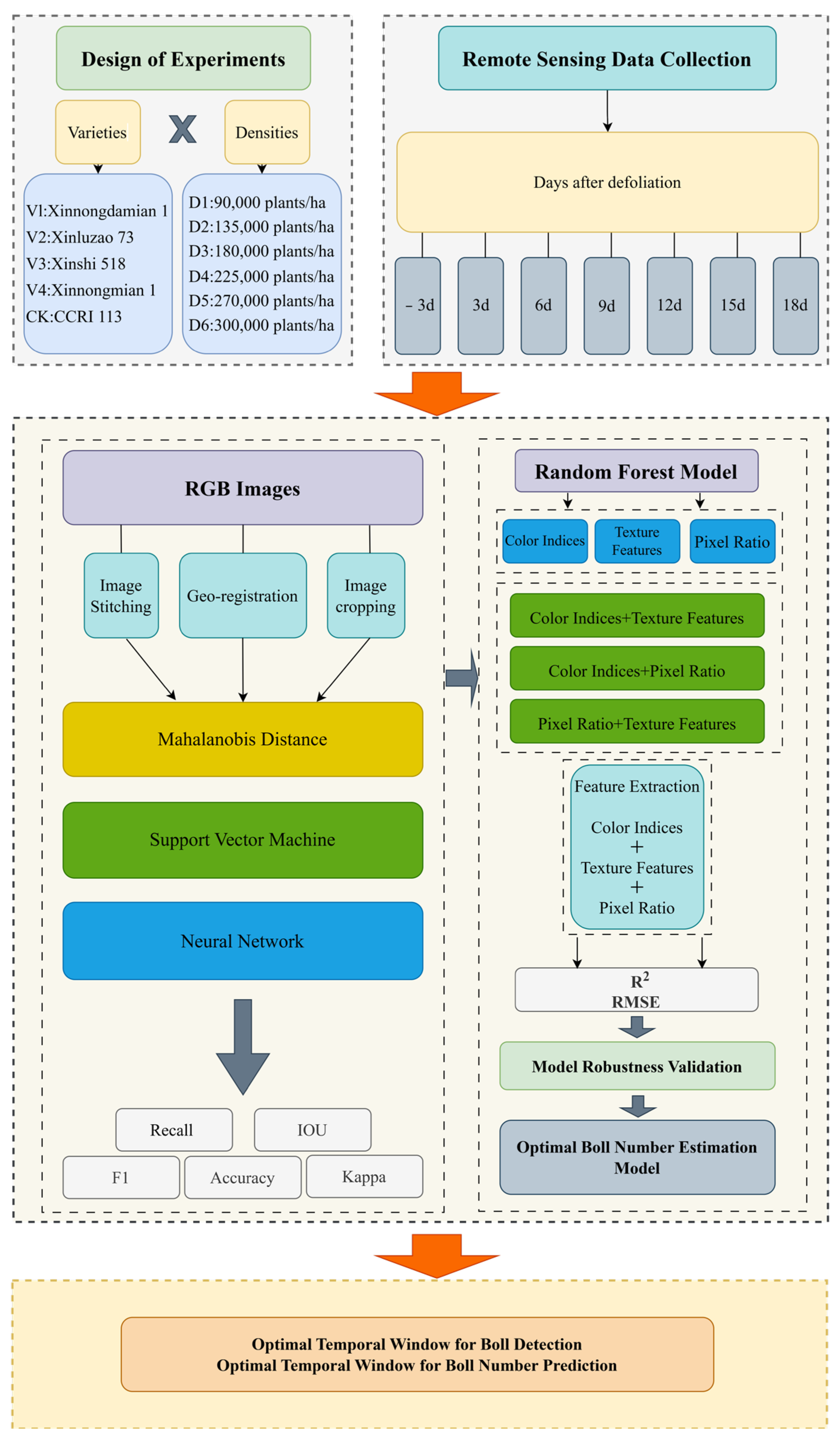
Although remote sensing techniques have been widely applied to cotton yield monitoring, accurate cotton boll extraction and boll number prediction still face several critical bottlenecks, particularly when imagery acquired on different days before and after defoliation must be systematically evaluated and translated into an operational monitoring window. The core challenges include: (1) how to overcome the three-dimensional canopy occlusion of cotton plants to achieve accurate extraction of bolls in the middle and lower canopy; (2) under the coexistence of multiple remote-sensing feature sources, how to construct reliable feature fusion models to stably improve the robustness of boll number estimation; and (3) given the dynamic canopy structural changes induced by defoliant application, what trade-off exists between decreasing leaf occlusion and increasing exposure of background elements over time, and how this trade-off affects cotton boll extraction and boll number estimation, thereby determining the optimal temporal window for prediction. To address these questions, this study uses multi-temporal UAV visible-light imagery to evaluate the performance of machine-learning algorithms for automatic cotton boll extraction and to quantify the effects of defoliation practices on boll extraction and boll number estimation. Specifically, boll extraction serves as the basis for deriving exposure-related features, which are then used as key inputs to subsequent boll number estimation under a feature fusion framework. The response variable in this study is the final boll number per plant measured near harvest, and images acquired on different dates are treated as alternative sources of predictive information for the same target, enabling a direct comparison of predictive performance over time and the identification of the most reliable observation window. The workflow of this study is shown in Figure 1.

2. Materials and Methods

2.1. Study Area Description and Experimental Design

2.1.1. Study Area Description

This study was conducted in 2024 at Huaxing Farm in Changji City, Xinjiang Uygur Autonomous Region, China (44°13′ N, 87°18′ E). The region has an elevation of 428 m and is characterized by a semi-arid continental climate, with an average annual sunshine duration of 2700 h, mean annual precipitation of approximately 190 mm, mean annual evaporation of approximately 1787 mm, and a mean annual air temperature of 6.8 °C. The recorded maximum and minimum temperatures are 42 °C and −38.2 °C, respectively. The frost-free period is 170 days, and the accumulated temperature above 10 °C is 3450 °C.

2.1.2. Experimental Design

The experiment followed a two-factor randomized complete block design, with cultivar and planting density as the two factors, to enhance the applicability of the estimation models under different scenarios. The tested cultivars were Xinnongda Cotton No. 1 (V1), Xinluzao 73 (V2), Xinshi 518 (V3), and Xinnong Cotton No. 1 (V4). Planting density was set at 90,000 plants ha⁻¹ (D1), 135,000 plants ha⁻¹ (D2), 180,000 plants ha⁻¹ (D3), 225,000 plants ha⁻¹ (D4), and 270,000 plants ha⁻¹ (D5), corresponding to plant spacings of 29.2 cm, 19.5 cm, 14.6 cm, 11.7 cm, and 9.7 cm, respectively. The core experiment was a balanced full-factorial combination in which cultivars V1–V3 were crossed with densities D1–D5, resulting in 15 cultivar × density treatments (3 × 5). These treatments were replicated three times (three blocks), yielding 45 plots. In addition, to evaluate model extrapolation to a new genotype, cultivar V4 was included under D1–D5; due to limited field space, only one replicate was established (five plots). Five control (CK) plots were also included. In total, 55 plots were established. Each plot covered an area of 6.0 × 9.0 m. Sowing was conducted on 28 April 2024 using a “one film, three drip lines, six rows” planting pattern, with a row-spacing configuration of (10 + 66 + 10 + 66 + 10 + 66) cm. Other management practices followed local standard recommendations.

2.2. Data Collection

2.2.1. Cotton Boll Number Data Acquisition

When the boll opening rate exceeded 80%, boll number was surveyed. During the field survey, three sampling quadrats (2.3 × 2.9 m) were randomly selected within each plot. The number of plants and bolls within each quadrat was recorded, and the mean boll number per plant was calculated. This plot-level boll number per plant was measured once near harvest and was used as the unified ground-truth observation for all subsequent modeling. For each UAV image acquisition date, plot-level image features were extracted and an independent date-specific estimation model was developed to predict the same target, enabling a direct comparison of predictive performance across dates.

2.2.2. UAV System and Remote Sensing Data Acquisition

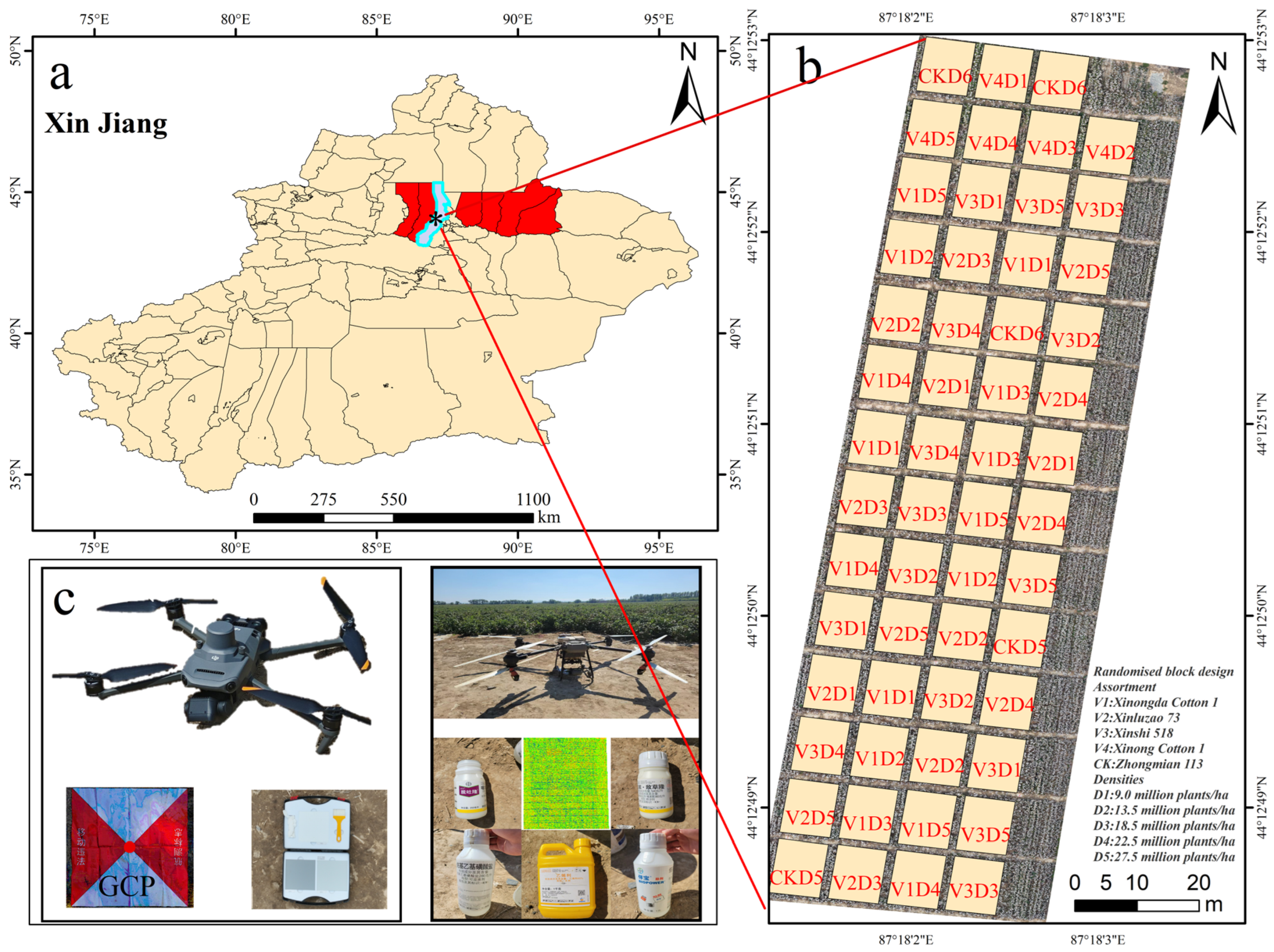
In this study, the DJI Mavic 3M multispectral UAV (DJI, Shenzhen, China) was used as the data acquisition platform. This model is equipped with a newly developed imaging system integrating one 20-megapixel RGB camera and four 5-megapixel multispectral cameras. The multispectral bands include green, red, red edge, and near-infrared wavelengths, enabling the simultaneous acquisition of high-resolution RGB and multispectral imagery. The UAV system is shown in Figure 2c.

The flight altitude was set to 30 m. UAV image acquisition was conducted at 3 days before defoliant application and at the 3rd, 6th, 9th, 12th, 15th, and 18th days after application, corresponding to the dates of 5 September, 11 September, 14 September, 17 September, 20 September, 23 September, and 26 September, respectively. Defoliation was carried out using a commercial thidiazuron-based defoliant (Bayer Crop Science (China) Co., Ltd., Hangzhou, China) following local practice. Efforts were made to ensure clear, windless, and cloud-free weather conditions, and all flights were carried out between 13:00 and 15:00 Beijing time. Prior to the first image acquisition, 6–10 ground control targets were evenly distributed across each experimental field and fixed in place with nails; their positions were documented and kept unchanged for all subsequent UAV missions. The defoliant application procedure and the layout of the ground control targets are shown in Figure 2c.

2.3. Data Processing and Analysis

2.3.1. Image Preprocessing

Visible-light image mosaicking: In this study, image mosaicking was performed using Metashape software (version 2.0.4, Agisoft LLC, St. Petersburg, Russia). First, the RGB images were imported and camera parameters were calibrated. Subsequently, photographs of the ground control targets were imported and control points were set to establish a geometric reference. Next, photo alignment and optimization were conducted to achieve accurate image matching and parameter refinement. Finally, a batch-processing workflow was initiated to sequentially generate the dense point cloud, digital elevation model, and orthomosaic, and the corresponding outputs and quality reports were exported.

Georeferencing: The visible-light images were georeferenced using the “Georeferencing” tool in ArcGIS 10.8 software (Esri, Redlands, CA, USA). The images were imported into ArcMap, and the RGB orthomosaic was used as the basemap. The “Georeferencing” tool was then opened, and control points were added using the centers of the ground control targets as coordinates. Finally, the georeferencing was updated.

2.3.2. Cotton Boll Extraction

All three extraction algorithms were implemented on the ENVI platform (version 5.6, EXELIS., Boulder, CO, USA). First, cotton bolls and background samples were delineated on the RGB images using the ROI tool, and 50 cotton boll ROIs and 50 background ROIs were selected within the experimental plots as supervised classification samples. Boll ROIs were chosen from visually identifiable, well-exposed bolls with clear boundaries, whereas background ROIs were sampled to represent major non-boll components. Care was taken to ensure that pixels within each ROI exhibited relatively consistent spectral and textural characteristics, thereby reducing the influence of mixed pixels. To standardize ROI selection across acquisition dates, we applied the same delineation criteria and fixed the ROI numbers for each date, and distributed ROIs across multiple plots to capture variability in illumination and canopy structure. These ROIs were used as training samples, and the Mahalanobis distance, support vector machine, and neural network modules in ENVI were applied for supervised classification to generate boll/non-boll maps. Accuracy assessment was performed using an independent validation area (CK, 23 September) within the same orthomosaic that was not used for ROI selection, training, or parameter tuning. In CK, an independent set of 50 boll ROIs and 50 background ROIs was delineated for validation only, based on which confusion matrices were exported and accuracy metrics were calculated.

(1)

The Mahalanobis distance (MD) is a supervised classification method based on the covariance matrix. By normalizing the feature space, it simultaneously accounts for the correlations among features in the distance metric, making it suitable for handling highly correlated and high-dimensional remote-sensing spectral features [22].

(2)

Support vector machine (SVM) is a margin-based supervised classifier that constructs an optimal separating hyperplane in a high-dimensional feature space, and nonlinear class boundaries can be modeled through kernel functions. In this study, boll extraction using SVM was implemented with the SVM supervised classification module in ENVI, trained with two ROI classes (boll and background). The radial basis function (RBF) kernel was selected (Kernel Type = Radial Basis Function), with γ = 0.333 (Gamma in Kernel Function = 0.333) and a penalty parameter C = 100 (Penalty Parameter = 100.000). Multi-scale processing was not used (Pyramid Levels = 0), and the classification probability threshold was set to 0.00. The classification outputs were written to file, and rule images were exported (Output Rule Images = Yes) for subsequent evaluation [23].

(3)

Neural networks (NN) consist of interconnected nonlinear units organized in layers, and the network weights are iteratively updated by backpropagation to learn a nonlinear mapping from input features to output classes. In this study, boll extraction was implemented using the Neural Network supervised classifier in ENVI, which corresponds to a feedforward multilayer perceptron (MLP) trained on user-defined ROIs (boll vs. background). The classifier was configured with one hidden layer and a logistic activation function, and trained for up to 1000 iterations with a learning rate of 0.20 and momentum of 0.90; the training threshold contribution and RMS exit criterion were set to 0.90 and 0.10, respectively. These settings enable the classifier to flexibly model nonlinear separations between boll and background classes under the rapidly changing canopy conditions during defoliation, thereby improving the robustness of boll extraction [24].

2.3.3. Cross-Platform Data Flow

The orthomosaics generated in Metashape and georeferenced in ArcGIS were further clipped into plot-level subsets in ArcGIS to ensure consistent spatial alignment across acquisition dates. The plot-level images were then imported into ENVI for ROI delineation and supervised classification, producing the classified mask maps. Based on the classification outputs, the boll pixel ratio was computed and plot-level color indices and texture metrics were extracted and compiled into a feature table, which was exported for subsequent date-specific boll number estimation and evaluation.

2.3.4. Remote Sensing Feature Extraction

(1)

Cotton Lint Pixel Ratio

In this study, the cotton pixel ratio was calculated based on the classification results obtained from the neural network model and was used as one of the key feature variables for boll number estimation. The calculation of the cotton pixel ratio is shown in the following equation, where P_r represents the cotton pixel ratio, P_c denotes the number of cotton pixels in the image, and P_t denotes the total number of pixels in the image.

$${\mathrm{P}}_{\mathrm{r}}={\displaystyle \frac{{\mathrm{P}}_{\mathrm{c}}}{{\mathrm{P}}_{\mathrm{t}}}}$$

(1)

(2)

Cotton Boll Texture Feature Extraction

Because the gray-level co-occurrence matrix (GLCM) can extract features such as contrast, energy, correlation, and homogeneity, and as a gray-level invariant feature extraction method it is not affected by image brightness, color, or illumination conditions, it can adapt to different acquisition environments and effectively improve the robustness and accuracy of cotton boll number estimation models. In this study, three texture features were extracted, including correlation (Correlation), entropy (Entropy), and mean (Mean), and their calculation methods are shown in Equation.

$$\mathrm{Correlation}={\displaystyle \frac{{\sum }_{\mathrm{i},\mathrm{j}}\left(\mathrm{i}-\overline{\mathrm{i}}\right)\left(\mathrm{j}-\overline{\mathrm{j}}\right)\mathrm{P}\left(\mathrm{i},\mathrm{j}\right)}{\sqrt{{\sum }_{\mathrm{i},\mathrm{j}}{\left(\mathrm{i}-\overline{\mathrm{i}}\right)}^2\mathrm{P}\left(\mathrm{i},\mathrm{j}\right){\sum }_{\mathrm{i},\mathrm{j}}{\left(\mathrm{j}-\overline{\mathrm{j}}\right)}^2\mathrm{P}\left(\mathrm{i},\mathrm{j}\right)}}}$$

(2)

$$\mathrm{Entropy}=-{\sum }_{\mathrm{i},\mathrm{j}}\mathrm{P}\left(\mathrm{i},\mathrm{j}\right)\log \left(\mathrm{P}\left(\mathrm{i},\mathrm{j}\right)\right)$$

(3)

$$\mathrm{Mean}={\displaystyle \frac{{\sum }_{\mathrm{i},\mathrm{j}}\mathrm{i}\mathrm{P}\left(\mathrm{i},\mathrm{j}\right)}{{\sum }_{\mathrm{i},\mathrm{j}}\mathrm{P}\left(\mathrm{i},\mathrm{j}\right)}}$$

(4)

(3)

Cotton Boll Spectral Feature Extraction

The RGB indices used in this study are summarized in

Table 1. Summary of RGB Indices.

Vegetation Index	Formulas	References
r	R/(R + G + B)	/
g	G/(R + G + B)	/
b	B/(R + G + B)	/
EXG	2 × G − R − B	[25]
RGBVI	(G2 − R × B)/(G2 + R × B)	[26]
NGBDI	(G − B)/(G + B)	[27]
VDVI	(2G − R − B)/(2G + R + B)	[28]

.

2.3.5. Developing the Cotton Boll Estimation Model

The model was implemented in Python (v3.10), with the regression framework constructed using scikit-learn (v1.6.1). First, the input features were standardized, and second-order interaction polynomial feature expansion was applied to enhance the representation of nonlinear relationships and feature interactions; subsequently, feature importance was estimated using a random forest, and features with higher contributions were retained for modeling through threshold-based selection. During model construction, the dataset was divided into training and testing sets at a ratio of 8:2, and key hyperparameters were jointly optimized on the training set using five-fold cross-validation combined with grid search, with the mean coefficient of determination (R²) from cross-validation used as the criterion for model selection.

2.3.6. Accuracy Assessment of Cotton Boll Extraction

(1)

Recall(R): Recall is used to measure the completeness of target detection by the model. It represents the proportion of correctly detected target pixels relative to all target pixels actually present in the image. A higher recall indicates fewer missed targets and a more comprehensive coverage of the target regions [29].

(2)

Intersection over Union (IOU): IOU is used to measure the degree of overlap between the extracted results and the ground-truth regions. It is calculated as the ratio of the intersection to the union of the extracted region and the corresponding ground-truth region. A higher value indicates better agreement between the extracted results and the true boundaries [30].

(3)

F1-score (F1): The F1-score is used to comprehensively evaluate precision and recall, and is essentially their harmonic mean, penalizing both false detections and missed detections simultaneously. In semantic extraction tasks, the F1-score is equivalent to the Dice coefficient, with values ranging from (0, 1), where higher values indicate better extraction performance [31].

(4)

Accuracy: Accuracy reflects the proportion of all pixels that are correctly classified by the model. It represents the ratio of correctly extracted pixels to the total number of pixels. A higher accuracy indicates better overall extraction performance [32].

(5)

Kappa coefficient (Kappa): The Kappa coefficient evaluates the agreement between the extraction results and the ground-truth labels. It corrects for agreement that may occur purely by chance. A Kappa coefficient closer to 1 indicates a higher level of agreement between the extracted results and the ground truth beyond random consistency [33].

2.3.7. Accuracy Evaluation of Boll Number Estimation Based on UAV RGB Imagery

In this study, the coefficient of determination (R²) and the relative root mean square error (rRMSE) were used to evaluate the goodness of fit and prediction accuracy of the model, and their calculation methods are shown in the following equations:

$${\mathrm{R}}^2 = 1 - {\displaystyle \frac{\sum _{\mathrm{i}=1}^{\mathrm{n}} {\left({\mathrm{y}}_{\mathrm{i}}-{\widehat{\mathrm{y}}}_{\mathrm{i}}\right)}^2}{\sum _{\mathrm{i}=1}^{\mathrm{n}} {\left({\mathrm{y}}_{\mathrm{i}}-\overline{\mathrm{y}}\right)}^2}}$$

(5)

$$\mathrm{rRMSE}(\%)={\displaystyle \frac{\mathrm{RMSE}}{\overline{\mathrm{y}}}} \times 100$$

(6)

where y_i represents the measured cotton boll number of the ith sample, ŷ_i denotes the predicted value, ȳ represents the mean of the measured values, and n is the number of samples.

3. Results

3.1. Analysis of Cotton Boll Identification Accuracy at Different Defoliation Stages Based on UAV RGB Imagery

As shown in

Table 2. Performance metrics of three cotton fiber segmentation models.

Date	Boll Extraction Algorithm	R (%)	F1	IOU (%)	Accuracy (%)	Kappa
9.05	MD	90.45	0.87	77.51	84.85	0.685
	SVM	95.28	0.90	81.32	87.36	0.735
	NN	74.55	0.84	71.82	87.64	0.739
9.11	MD	91.96	0.87	77.33	86.84	0.737
	SVM	91.60	0.88	77.79	87.23	0.745
	NN	98.32	0.90	81.23	88.91	0.779
9.14	MD	96.03	0.94	89.19	93.40	0.865
	SVM	96.03	0.94	89.13	93.36	0.864
	NN	89.97	0.94	88.73	93.52	0.870
9.17	MD	94.74	0.94	89.21	93.57	0.869
	SVM	94.45	0.95	90.91	94.70	0.893
	NN	95.53	0.95	91.00	94.70	0.892
9.20	MD	95.66	0.95	89.75	93.73	0.871
	SVM	95.00	0.96	91.86	95.16	0.901
	NN	94.34	0.96	92.76	95.77	0.914
9.23	MD	97.04	0.96	92.23	94.77	0.885
	SVM	97.55	0.96	93.17	95.42	0.890
	NN	99.18	0.96	93.01	95.23	0.894
9.26	MD	92.69	0.94	89.04	93.42	0.866
	SVM	92.68	0.94	89.03	95.16	0.900
	NN	91.11	0.95	90.09	95.75	0.912
CK (9.23)	MD	90.08	0.92	85.55	92.26	0.845
	SVM	98.34	0.99	97.86	98.90	0.980
	NN	97.68	0.99	97.52	98.73	0.975

“MD”, “SVM”, and “NN” denote the Mahalanobis distance method, support vector machine, and neural network, respectively. CK (23 September) denotes an independent validation area (an adjacent cotton field within the same orthomosaic) that was not used for ROI selection, classifier training, or parameter tuning; CK metrics were computed using 50 boll ROIs and 50 background ROIs delineated in the CK area and are reported for this date only.

, the neural network outperformed the other two algorithms in terms of consistency metrics at most key periods, with particularly strong performance in the middle and late stages. For example, the Kappa coefficient reached 0.914 on 20 September and 0.912 on 26 September, indicating a stronger capability of the neural network to capture fine texture details and nonlinear class separability under complex background conditions. The support vector machine ranked second in the classification task and exhibited relatively stable performance across all periods, with more pronounced boundary overlap at certain time points; for instance, the intersection over union reached 93.17% and the Kappa coefficient reached 0.890 on 23 September. The Mahalanobis distance achieved relatively high recall at some key periods, with a recall of 97.04% on 23 September; however, its Kappa coefficients were generally lower than those of the support vector machine and neural network, such as 0.871 on 20 September compared with 0.914 for the neural network. This indicates that the Mahalanobis distance method tends to confuse exposed soil and senescent leaves with cotton bolls, resulting in reduced consistency and boundary stability. Importantly, the independent area validation conducted on 23 September (CK) further corroborated the robustness ranking among algorithms under non-experimental field conditions. In CK, SVM and the neural network maintained very high agreement and boundary consistency (F1 = 0.99; IOU = 97.86% and 97.52%; Kappa = 0.980 and 0.975, respectively), whereas the Mahalanobis distance exhibited noticeably lower agreement (Kappa = 0.845; IOU = 85.55%), suggesting a higher susceptibility to background-induced false positives when transferred to an independent field area.

From a temporal perspective, the accuracies of all three algorithms exhibited a stage-wise improvement with the progression of defoliation: performance was relatively low on 5 September, began to improve by 14 September, and reached higher values and became stable from 20 September to 26 September.

As shown in

Table 3. Computational efficiency of the three extraction algorithms.

Three Extraction Algorithms	Time (s)
MD	1.60
SVM	1.80
NN	2.70

, for the same imagery, the single-run computation times of the Mahalanobis distance and support vector machine were 1.60 s and 1.80 s, respectively, whereas that of the neural network was 2.70 s, indicating relatively lower computational efficiency. However, in cotton boll extraction tasks, classification accuracy and result stability take precedence over second-level differences in computation time: the neural network outperformed the other models across evaluation metrics and effectively reduced the impact of missed detections on cotton boll extraction. Therefore, under an acceptable computational cost, priority was given to the neural network with higher accuracy and robustness.

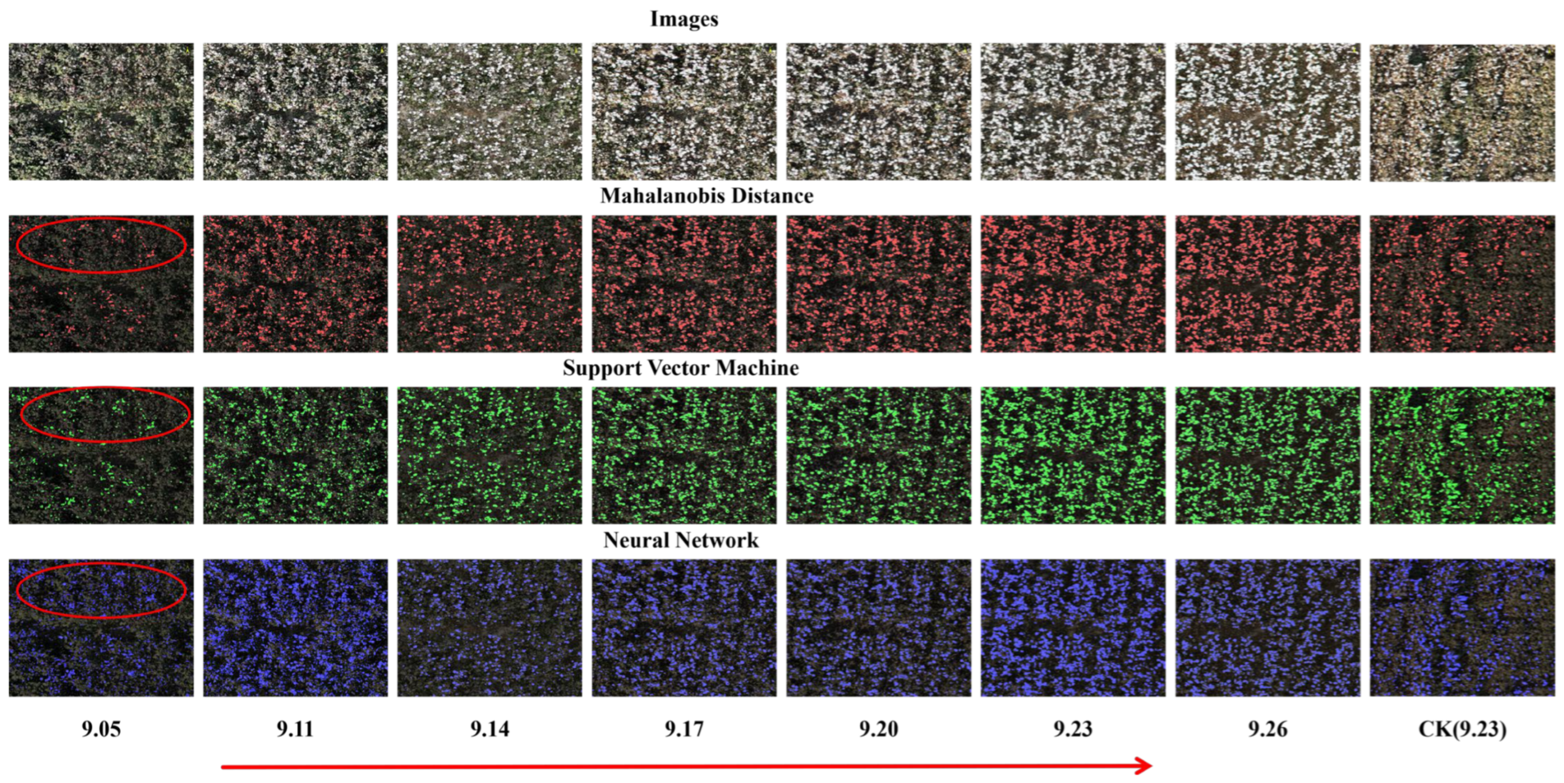
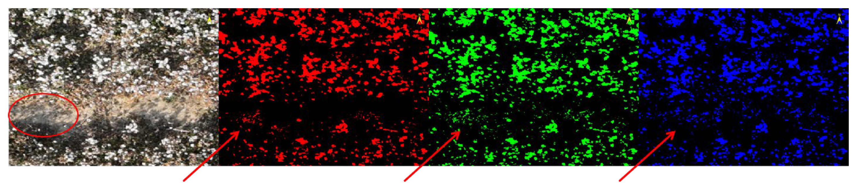
As shown in Figure 3, the red circled areas visually indicate that the neural network method achieved overall better performance in cotton boll target extraction than the Mahalanobis distance and support vector machine methods. Throughout the entire defoliation period, the number of cotton bolls extracted by the neural network was consistently higher than that obtained by the other two methods, indicating stronger classification capability for cotton boll targets and a lower rate of missed detections. Meanwhile, as indicated by the arrows from left to right in the figure, the number of cotton bolls extracted by all three methods exhibited a gradual increasing trend with the progression of defoliation, reflecting the consistently positive effect of leaf abscission and increased boll exposure on remote-sensing extraction results. Overall, the neural network demonstrated higher cotton boll extraction efficiency across different defoliation stages, providing relatively reliable feature inputs for subsequent calculation of the cotton bolls pixel ratio.

Figure 4 also illustrates a representative failure case under high-brightness plastic mulch. All three algorithms exhibit background-driven false positives to some extent, whereas SVM and the neural network show improved boundary consistency relative to the Mahalanobis distance classifier.

3.2. Cotton Boll Estimation at Different Defoliation Stages Based on UAV RGB Imagery

3.2.1. Effects of Different Cultivars and Planting Densities on Cotton Boll Number

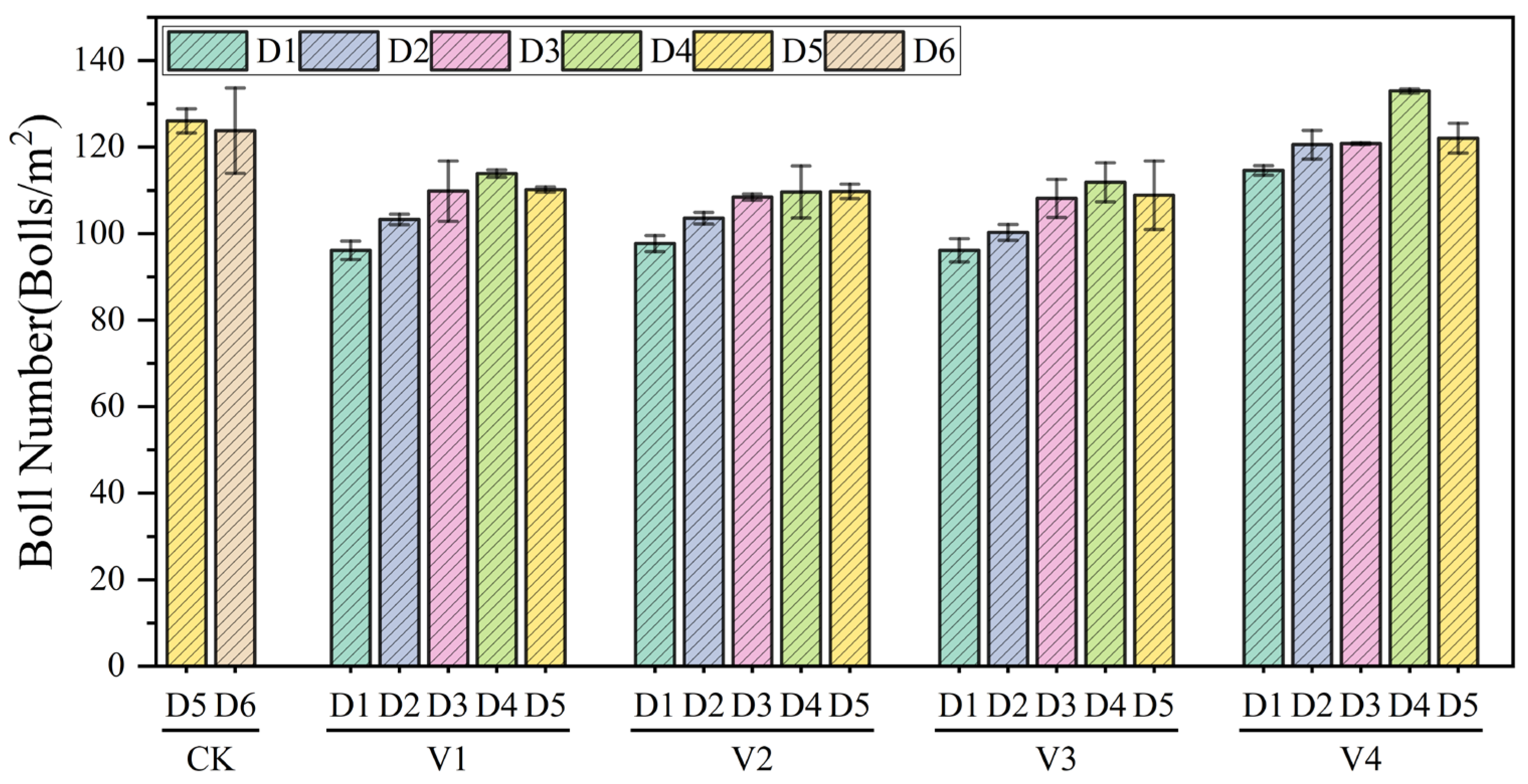
As shown in Figure 5, cultivar and planting density had significant effects on cotton boll number, with a clear interaction between the two factors, indicating that different cultivars responded differently to density gradients. Across cultivars, V4 exhibited the highest boll number, exceeding those of V1, V2, and V3 by 15.54, 16.39, and 17.13 bolls/m², respectively. In terms of planting density, the mean boll number across cultivars followed the trend D1 < D2 < D3 < D5 < D4, with the highest boll number observed at D4, representing an increase of 15.93 bolls/m² (approximately 15.8%) compared with D1. When planting density was further increased to D5, boll number began to decline, indicating that moderate increases in planting density can enhance boll number, whereas excessively high density may reduce boll retention due to intensified resource competition. Overall, the V4D4 combination achieved the highest boll number among all treatments, reaching 133.00 bolls/m², which was 10.95 bolls/m² (approximately 9.0%) higher than that under the V4D5 treatment. Collectively, under the conditions of this experiment, the V4 cultivar grown at medium-to-high planting densities was more favorable for increasing boll number per unit area.

3.2.2. Analysis of Cotton Boll Number Estimation at Different Defoliation Stages Based on UAV RGB Image Features

As shown in

Table 4. Accuracy evaluation of models based on single-source features.

Date	Color Indices		Texture Features		Pixel Ratio
	R2	rRMSE (%)	R2	rRMSE (%)	R2	rRMSE (%)
9.05	0.0005	9.40	0.0075	9.40	0.0155	9.40
9.11	0.0379	9.20	0.1873	8.50	0.0070	9.40
9.14	0.0473	9.20	0.0924	9.00	0.0448	9.20
9.17	0.0292	9.30	0.0112	9.40	0.4204	7.20
9.20	0.1352	8.80	0.0378	9.20	0.2624	8.10
9.23	0.2128	8.40	0.4037	7.30	0.3740	7.50
9.26	0.6156	5.80	0.1399	8.70	0.1637	8.60

, boll number estimation models driven by single features did not exhibit a clear monotonic trend with increasing dates in the time series, but instead fluctuated with the progression of defoliation, indicating that the performance of single-feature-based models is highly sensitive to leaf occlusion, background exposure, and variations in image characteristics. From the perspective of the defoliation process, during the period from 6 September to 14 September, all three types of features showed generally weak performance, with R² values mostly ranging from 0 to 0.05 and rRMSE values between 9.2% and 9.4%. On 17 September, the model constructed using the pixel ratio showed a marked improvement in accuracy and reached a stage-specific peak during the defoliation period (R² = 0.4204, rRMSE = 7.2%). Subsequently, from 20 September to 23 September, the accuracies of the models driven by color indices and texture features began to improve, with the texture-based model reaching its optimum on 23 September (R² = 0.4037, rRMSE = 7.3%). On 26 September, the color index-driven model achieved its highest accuracy (R² = 0.6156, rRMSE = 5.8%), while the accuracies of the models driven by cotton boll pixel ratio and texture features declined. Overall, models driven by individual image features were prone to performance fluctuations influenced by the defoliation process, and no clear or consistent temporal pattern in model accuracy was observed across the time series.

3.2.3. Construction of Multi-Feature Fusion Boll Number Estimation Models

As shown in

Table 5. Accuracy evaluation of models based on dual-source feature fusion.

Date	Color Indices + Texture Features		Color Indices + Pixel Ratio		Pixel Ratio + Texture Features
	R2	rRMSE (%)	R2	rRMSE (%)	R2	rRMSE (%)
9.05	0.0218	9.30	0.0012	10.29	0.0753	9.90
9.11	0.2550	8.10	0.1534	8.70	0.2202	9.09
9.14	0.2266	8.30	0.0626	9.97	0.1909	9.26
9.17	0.0360	9.30	0.6011	6.00	0.4611	6.90
9.20	0.1089	8.90	0.4664	6.90	0.4832	6.80
9.23	0.6258	5.80	0.5650	6.79	0.4654	6.90
9.26	0.6965	5.20	0.6621	5.50	0.2844	8.71

, models driven by dual-feature combinations exhibited overall greater stability in estimation accuracy than those driven by single features. On 6 September, the accuracies of the three dual-feature combination models were still relatively low, with R² values ranging from 0.0012 to 0.0753 and rRMSE values between 9.3% and 10.3%. From 11 September to 14 September, model performance improved, with R² increasing to 0.1527–0.2550 and rRMSE decreasing to 8.1–9.9%, which was clearly superior to the performance of single-feature-driven models. From 17 September to 26 September, the fusion models generally operated within a higher performance range, with R² values mostly between 0.4634 and 0.6965 and rRMSE values between 5.2% and 6.9%, and were less prone to abrupt accuracy fluctuations at specific time points compared with single-feature models. This improvement can be attributed to the fact that the two feature types capture different signal dimensions: one reflects canopy color variation, while the other quantifies structural differences, and their integration enhances the model’s adaptability to leaf occlusion and background changes during the defoliation process. Overall, dual-feature fusion models effectively improved the stability of model performance under dynamic image characteristics associated with defoliation, thereby maintaining relatively high boll number estimation accuracy throughout the defoliation period.

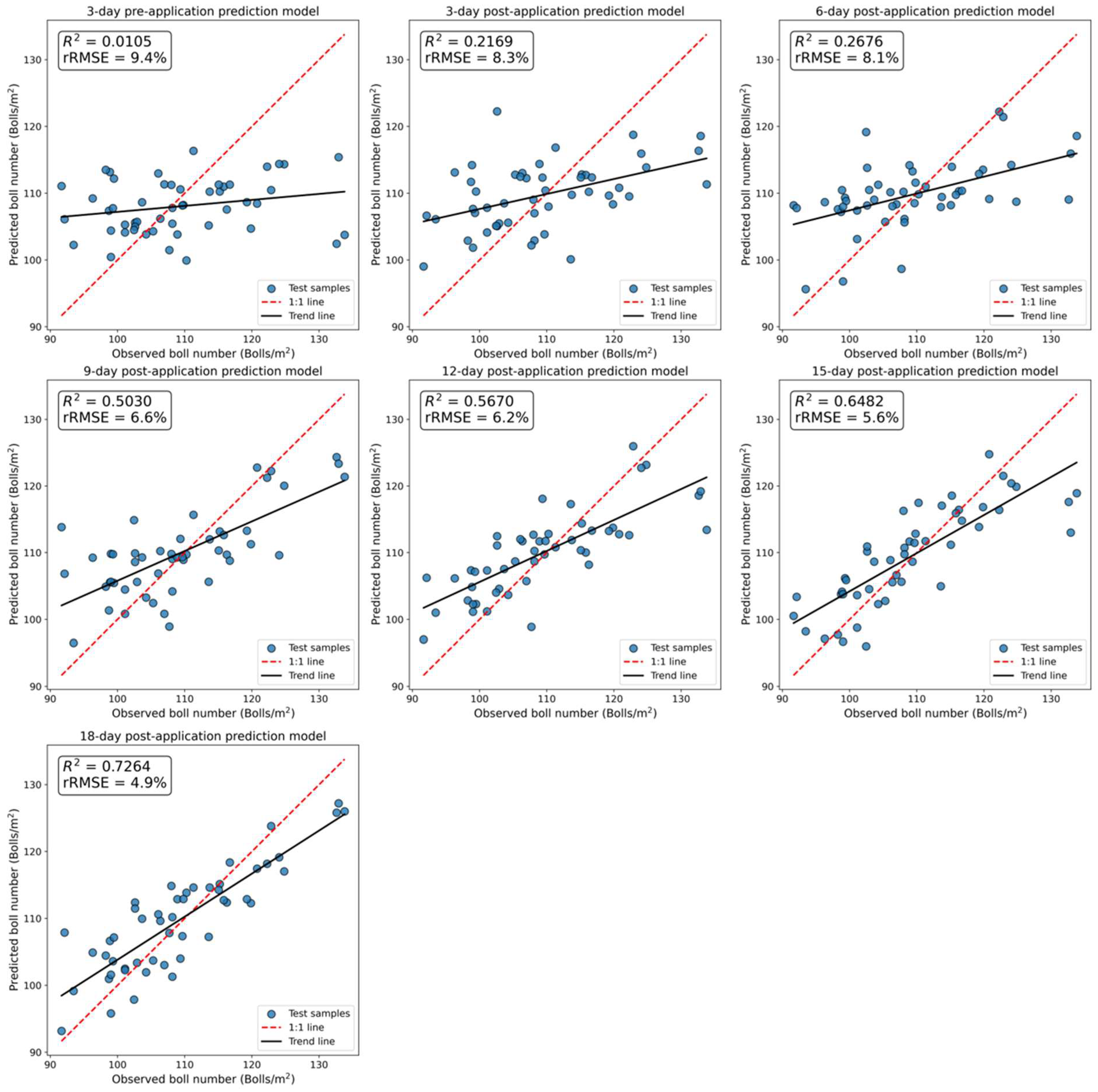
As shown in Figure 6, the boll number estimation model integrating three image features achieved the highest estimation accuracy during the middle and late stages and exhibited a gradual increasing trend over the time series. On 6 September, the multi-feature fusion model showed a coefficient of determination of 0.0105 and an rRMSE of 9.4%, indicating that the model had almost no explanatory capability. From 11 September to 20 September, the coefficient of determination generally ranged between 0.2169 and 0.5670, while the rRMSE decreased from 8.3% to 6.2%, suggesting that the boll number estimation model had developed a certain fitting ability during this period and that prediction errors became relatively convergent. As cotton bolls were further exposed and differences in canopy structure were more fully captured, a marked improvement in model performance was observed on 23 September and 26 September, with the coefficient of determination increasing to 0.6482 and 0.7264, respectively, and the rRMSE concurrently decreasing to 6.1092 and 5.3873. Overall, the accuracy of the multi-feature fusion model increased progressively with the advancement of defoliation and reached its optimum in the late defoliation stage, clearly demonstrating that multi-source remote-sensing feature fusion enhances the model’s adaptability to temporal variations and treatment differences, thereby exhibiting improved robustness.

3.3. Robustness Validation of the Boll Number Estimation Model

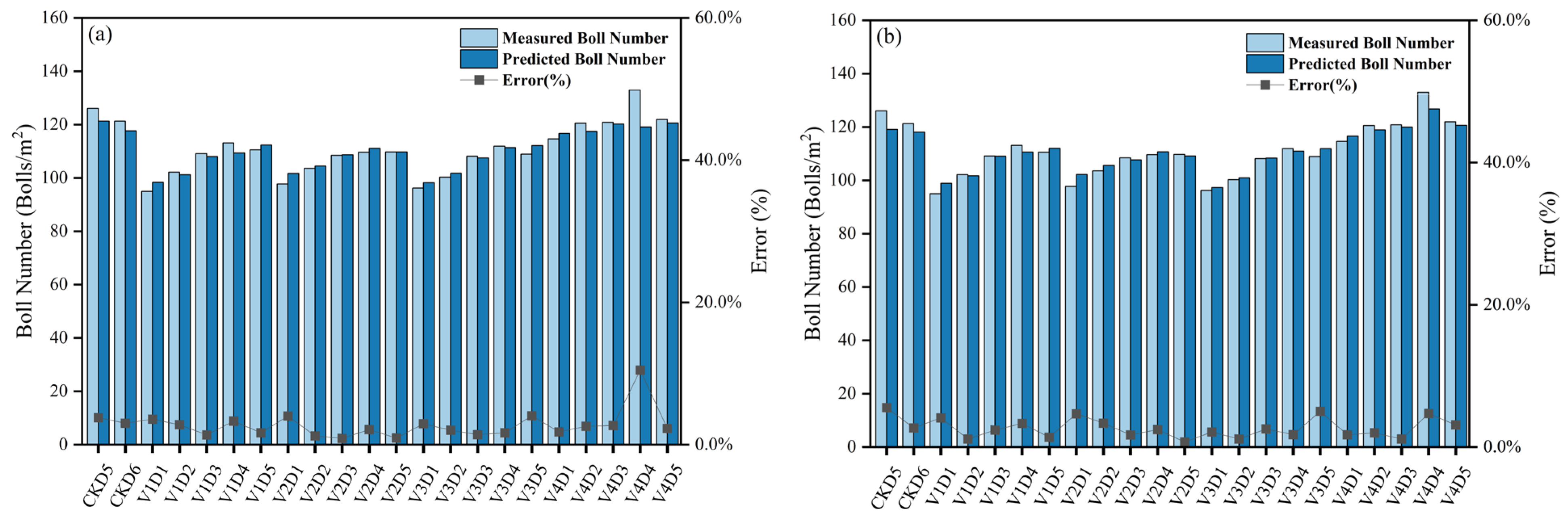
As shown in Figure 7, the boll number estimation model developed in this study exhibited overall stable performance in the robustness validation on 23 September and 26 September. For both dates, the estimated values generally varied in close agreement with the measured values across treatments, with relatively small differences in bar heights for most treatments. The errors were below 5%, with mean errors of approximately 2.76% and 2.67%, respectively, and no systematic overestimation or underestimation was observed with increasing boll number levels. On 23 September, a noticeable underestimation occurred only for the V4D4 treatment, with an error of 10.47%, whereas errors for the remaining treatments were mostly within 0.89–4.05%. The error distribution on 26 September was more uniform, with a maximum error of approximately 5.54%. Overall, these results indicate that the model shows good adaptability to changes in canopy structure and boll exposure during the late defoliation stage, although underestimation may still occur under conditions of higher-density boll number distributions.

4. Discussion

4.1. Effects of Different Machine Learning Algorithms on Cotton Lint Extraction Accuracy at Different Stages Before and After Defoliation

Recent studies have shown that cotton boll opening and its remote-sensing characteristics are strongly influenced by canopy structure and leaf occlusion at different boll-opening stages; in the early stage, cotton bolls are easily obscured by upper canopy leaves, whereas they become progressively exposed as defoliation advances, resulting in pronounced differences in extraction difficulty among stages [34]. Other studies have demonstrated that under natural illumination and complex field background conditions, leaf occlusion, shadows, and brightness variations can significantly disturb the stability of color and texture features, and traditional image-processing approaches that rely on color and texture thresholds therefore often suffer from missed detections at the field scale and fail to ensure cotton boll extraction accuracy, a problem that is particularly pronounced during the pre-defoliation stage when foliage is abundant.

The Mahalanobis distance classifier, as a linear supervised classification method based on within-class covariance, has achieved relatively high accuracy in leaf segmentation from agricultural RGB imagery [35], but this method is highly dependent on sample statistical distributions and stable spectral differences, and is prone to class confusion under complex canopy structures and high background noise, which limits its field applicability. In contrast, support vector machines that integrate color and geometric features have been successfully applied to cotton boll identification and counting from RGB remote-sensing imagery, maintaining relatively high pixel-level classification accuracy and boll counting accuracy under different management practices [36]. For example, Naveen et al. used an SVM classifier based on GLCM texture features for leaf identification and showed that SVM could maintain relatively stable classification performance when multidimensional texture information was incorporated [37]. The advantage of such algorithms lies in their strong adaptability to small sample sizes, making them suitable for relatively simple scenarios; however, their reliance on manually designed features makes it difficult to maintain robustness under complex field illumination conditions.

In recent years, deep convolutional neural networks have gradually become the dominant technical approach for cotton boll extraction: Singh et al. employed fully convolutional networks to achieve semantic segmentation of cotton bolls from aerial perspectives, achieving intersection-over-union values exceeding 90% under conditions where cotton bolls were highly mixed with sky and background elements [38]. Convolutional neural networks can automatically learn multi-level feature representations, and lightweight fully convolutional networks have been further developed that reduce parameter counts and inference time by approximately half while still maintaining cotton boll pixel accuracies above 98% and IOU values of around 91%, making them suitable for real-time deployment on airborne and embedded platforms [39]. Bairi et al. optimized cotton boll detection performance using multi-scale attention mechanisms, improving small-target recognition accuracy while maintaining detection speed, thereby demonstrating the adaptability of deep models in high-contrast field environments [40].

Stage-dependent differences among algorithms in this study were consistent with typical background interferences during defoliation. In the pre-defoliation stage and the early post-defoliation stage, canopy occlusion and related factors weaken the visible boll signal, thereby increasing missed detections. During the mid-defoliation stage, greater exposure of bare soil and plastic mulch, together with enhanced localized specular reflections, increases false positives; under high background noise, the Mahalanobis distance method is more prone to class confusion because it relies on within-class statistical distributions and stable spectral separability. This background-driven error pattern is also illustrated by the representative high-brightness plastic-mulch case in Figure 4, where false positives occur across methods but are more pronounced for the Mahalanobis distance classifier. By contrast, SVM and the neural network better discriminate bolls from background in a multidimensional feature space and maintained higher agreement and boundary stability in the independent field validation. Although CNN-based models can typically achieve higher segmentation accuracy when supported by large-scale annotations and sufficient computational resources, for the application scenario considered here, the ENVI-based supervised workflow combined with interpretable features offers practical advantages in terms of lower annotation cost, reproducibility, and rapid deployment, supporting both observation window identification and yield estimation. Future work will integrate pseudo-labeling and lightweight deep models to further improve cross-field and interannual generalization.

4.2. Effects of Days Before and After Defoliation on Boll Number Estimation and the Optimal Time Window for Boll Number Estimation

In this study, the performance differences in the cotton boll number estimation model mainly stem from two coupled factors: the temporal evolution of boll exposure during defoliation and the informational complementarity among different feature types. Before defoliant application and in the early post-application stage, leaf occlusion and canopy shading severely constrain visible boll signals, which limits the discriminability of models relying solely on color indices or texture features. Consistent with this, single-feature results indicate that texture features exhibit higher explanatory power than color indices at the early stage: on 11 September, the texture-based model achieved an R² of 0.1873, whereas the color-index-based model only reached an R² of 0.0379. Fusing color indices with texture improved estimation stability, yielding an R² of 0.2550 and reducing rRMSE to 8.10% on 11 September. As defoliation progressed to the mid stage, boll exposure increased rapidly, while background components were simultaneously intensified, reducing target–background separability and causing stage-dependent fluctuations in estimation accuracy. At this transition stage, the boll pixel ratio became the dominant contributor once exposure increased; on 17 September, the pixel-ratio-based model achieved an R² of 0.4204 with an rRMSE of 7.20%. Combining the boll pixel ratio with color indices produced the largest accuracy gain, increasing R² to 0.6011 and decreasing rRMSE to 6.00%. In the late defoliation stage, boll exposure approached a relatively complete and stable state, and the characterization of canopy spatial heterogeneity by color indices and texture features became more consistent. Accordingly, color indices became the strongest single-feature predictor: on 26 September, the color-index-based model reached an R² of 0.6156 with an rRMSE of 5.80%, while fusing texture with color indices provided an additional and stable improvement (9.26: Color + Texture, R² = 0.6965 and rRMSE = 5.20%). More importantly, integrating all three feature sources led to a monotonic improvement in model performance throughout defoliation and achieved a stable high-accuracy regime in the late period (15–18 days after defoliant application: R² = 0.6482–0.7264 and rRMSE = 5.6–4.9%), thereby supporting the identified optimal observation window and highlighting the complementary roles of pixel ratio, color indices, and texture features. Consistent with this logic, previous studies have shown that multi-source feature fusion can enhance the estimation of yield differences, and that the joint use of multi-sensor information helps improve cotton yield estimation accuracy [41]. Better estimation performance is also more readily achieved in the late growth stage under high-density planting conditions [42]. Moreover, quantitatively extracting boll exposure after boll opening and incorporating its spatial distribution information into modeling can strengthen the explanatory power of remote-sensing features for yield differences, thereby improving yield estimation performance [43]. Integrating boll-related spatial distribution and structural information into model construction can further enhance the ability of image features to explain yield variability [44]. Image acquisition date has a significant effect on yield estimation errors, particularly during the period from boll opening to pre-harvest [45,46]. Therefore, jointly modeling late-season features with multi-temporal information is often more conducive to achieving robust predictive capability across fields [47,48]. In addition, ultra-high-resolution imagery acquired close to harvest has a stronger ability to discriminate fine-scale within-field yield differences [49].

4.3. Limitations and Future Directions

Although this study achieved relatively high accuracy in cotton boll extraction and boll number estimation, result stability is still affected by sample size, background heterogeneity, and labeling uncertainty. Boll extraction relied on a supervised ENVI workflow in which ROI selection and parameter tuning inevitably involve manual interaction; when samples are limited or soil/canopy conditions vary across fields, extraction errors may propagate to subsequent boll number estimation, increasing overfitting risk and accuracy fluctuations. Future work will explicitly evaluate field-scale spatial generalization by projecting plot-level residuals back onto the georeferenced orthomosaic and comparing different spatial zones, and by adopting spatially structured validation to reduce overly optimistic accuracy estimates caused by spatial autocorrelation. Because extraction accuracy in this study was assessed mainly using ROI-based references rather than pixel-wise ground-truth masks, future efforts will create manually annotated reference masks in representative sub-areas and reduce labeling uncertainty through double annotation and consensus, enabling more rigorous IOU/F1 evaluation, particularly for boundary-level errors. Moreover, this study used only visible-light imagery and did not concurrently measure key agronomic indicators such as defoliation rate and boll opening rate, which constrains mechanistic interpretation. Temporal validation was also limited: date-specific models were developed to predict the same near-harvest boll number per plant, and true time-forward generalization was not tested. Future work will expand datasets across more dates, regions, and years, implement time-forward validation and cross-field/cross-year transfer tests, and evaluate the interannual stability of the identified optimal observation window (15–18 days after defoliant application) and the feature fusion strategy; if systematic year-to-year drift is observed, transfer learning or domain adaptation will be explored to enable rapid adaptation to new seasons with limited labeled samples. Finally, integrating ground measurements with multi-source remote sensing data (e.g., multispectral, thermal infrared, and LiDAR) and exploring pseudo-labeling with lightweight deep models will help further improve robustness and scalability while reducing manual labeling effort.

5. Conclusions

Based on multi-temporal UAV visible-light imagery, this study developed cotton boll extraction and boll number estimation models for different days before and after defoliation, and identified the 15th and 18th days after defoliant application as the optimal observation windows for boll number estimation. In terms of boll extraction, the neural network consistently outperformed the Mahalanobis distance and support vector machine across all defoliation stages, achieving a maximum Kappa coefficient of 0.914 and providing relatively reliable target segmentation results for subsequent boll number prediction. The boll number estimation models driven by multiple features exhibited a clear temporal pattern: estimation accuracy was relatively low before defoliant application and in the early post-application stage, gradually increased during the middle stage, and reached higher and stable levels at the 15th and 18th days after application. The advantage of multi-feature fusion was more pronounced in the late defoliation period, with the coefficient of determination reaching 0.7264 and the root mean square error decreasing to 4.9% at the 18th day after application, indicating that jointly modeling the complementary information from color indices, texture features, and cotton boll pixel ratio enables a more comprehensive quantification of boll exposure and canopy structural changes in the late defoliation stage, thereby improving the stability and reliability of boll number estimation. Error structure analysis showed that the relative errors for most cultivar-density combinations were concentrated within 1–4%, with good performance at medium and medium-to-high densities, while a tendency toward underestimation persisted under extremely high density. After incorporating the cotton boll pixel ratio, the error distribution further converged, systematic biases in boll number estimation under high-density treatments were alleviated, and stability across cultivar and density gradients was simultaneously improved.

References

1. Zhang, Z.; Huang, J.; Yao, Y.; Peters, G.; Macdonald, B.; La Rosa, A.D.; Wang, Z.; Scherer, L. Environmental impacts of cotton and opportunities for improvement. Nat. Rev. Earth Environ. 2023, 4, 703–715. [Google Scholar] [CrossRef] [Scilit]
2. Zhao, X.; Zhu, A.L.; Liu, X.; Li, H.; Tao, H.; Guo, X.; Liu, J. Current status, challenges, and opportunities for sustainable crop production in Xinjiang. Science 2025, 28, 112114. [Google Scholar] [CrossRef] [Scilit] [PubMed]
3. Yang, Z.; He, C.; Wang, X.; Li, J.; Liang, X. Weather index insurance for transition to sustainable cotton production in Xinjiang, China. Front. Environ. Sci. 2022, 10, 1027260. [Google Scholar] [CrossRef] [Scilit]
4. Guo, S.; Liu, T.; Han, Y.; Wang, G.; Du, W.; Wu, F.; Li, Y.; Feng, L. Changes in within-boll yield components explain cotton yield variation across planting dates. Field Crops Res. 2023, 293, 108853. [Google Scholar] [CrossRef] [Scilit]
5. He, D.; Wang, E.; Kirkegaard, J.; Han, E.; Malone, B.; Swan, T.; Brown, S.; Glover, M.; Lawes, R.; Lilley, J. Usefulness of techniques to measure and model crop growth and yield at different spatial scales. Field Crops Res. 2024, 309, 109332. [Google Scholar] [CrossRef] [Scilit]
6. Aierken, N.; Yang, B.; Li, Y.; Jiang, P.; Pan, G.; Li, S. A review of unmanned aerial vehicle based remote sensing and machine learning for cotton crop growth monitoring. Comput. Electron. Agric. 2024, 227, 109601. [Google Scholar] [CrossRef] [Scilit]
7. Khanal, S.; Kushal, K.C.; Fulton, J.P.; Shearer, S.; Ozkan, E. Remote sensing in agriculture—Accomplishments, limitations, and opportunities. Remote Sens. 2020, 12, 3783. [Google Scholar] [CrossRef] [Scilit]
8. Liu, Q.; Zhang, Y.; Yang, G. Small unopened cotton boll counting by detection with MRF-YOLO in the wild. Comput. Electron. Agric. 2023, 204, 107576. [Google Scholar] [CrossRef] [Scilit]
9. Kamilaris, A.; Prenafeta-Boldú, F.X. Deep learning in agriculture: A survey. Comput. Electron. Agric. 2018, 147, 70–90. [Google Scholar] [CrossRef] [Scilit]
10. Liu, J.; Lai, H.; Jia, Z. Image segmentation of cotton based on YCbCr color space and Fisher discrimination analysis. Acta Agron. Sin. 2011, 37, 1274–1279. [Google Scholar] [CrossRef] [Scilit]
11. Fue, K.G.; Porter, W.M.; Rains, G.C. Deep learning based real-time GPU-accelerated tracking and counting of cotton bolls under field conditions using a moving camera. In Proceedings of the 2018 ASABE Annual International Meeting, Detroit, MI, USA, 29 July–1 August 2018; p. 1800831. [Google Scholar] [CrossRef] [Scilit]
12. Yeom, J.; Jung, J.; Chang, A.; Maeda, M.M.; Landivar, J. Automated open cotton boll detection for yield estimation using unmanned aircraft vehicle (UAV) data. Remote Sens. 2018, 10, 1895. [Google Scholar] [CrossRef] [Scilit]
13. Xia, M.; Chen, X.; Tian, X.; Wen, H.; Zhao, Y.; Liu, H.; Liu, W.; Zheng, Y. Lightweight deep learning for real-time cotton monitoring: UAV-based defoliation and boll-opening rate assessment. Agriculture 2025, 15, 2095. [Google Scholar] [CrossRef] [Scilit]
14. Xu, W.; Chen, P.; Zhan, Y.; Chen, S.; Zhang, L.; Lan, Y. Cotton yield estimation model based on machine learning using time series UAV remote sensing data. Int. J. Appl. Earth Obs. Geoinf. 2021, 104, 102511. [Google Scholar] [CrossRef] [Scilit]
15. Feng, A.; Zhou, J.; Vories, E.D.; Sudduth, K.A. Prediction of cotton yield based on soil texture, weather conditions and UAV imagery using deep learning. Precis. Agric. 2024, 25, 303–326. [Google Scholar] [CrossRef] [Scilit]
16. Wu, J.; Wen, S.; Lan, Y.; Yin, X.; Zhang, J.; Ge, Y. Estimation of cotton canopy parameters based on unmanned aerial vehicle (UAV) oblique photography. Plant Methods 2022, 18, 129. [Google Scholar] [CrossRef] [Scilit]
17. De Siqueira, D.A.B.; Vaz, C.M.P.; da Silva, F.S.; Ferreira, E.J.; Speranza, E.A.; Franchini, J.C.; Galbieri, R.; Belot, J.L.; de Souza, M.; Perina, F.J. Estimating cotton yield in the Brazilian Cerrado using linear regression models from MODIS vegetation index time series. AgriEngineering 2024, 6, 947–961. [Google Scholar] [CrossRef] [Scilit]
18. Rodriguez-Sanchez, J.; Li, C.; Paterson, A.H. Cotton yield estimation from aerial imagery using machine learning approaches. Front. Plant Sci. 2022, 13, 870181. [Google Scholar] [CrossRef] [Scilit]
19. Shi, G.; Du, X.; Du, M.; Li, Q.; Tian, X.; Ren, Y.; Zhang, Y.; Wang, H. Cotton yield estimation using the remotely sensed cotton boll index (DCP) from UAV images. Drones 2022, 6, 254. [Google Scholar] [CrossRef] [Scilit]
20. Huang, Y.B.; Sui, R.X.; Thomson, S.J.; Fisher, D.K. Estimation of cotton yield with varied irrigation and nitrogen treatments using aerial multispectral imagery. Int. J. Agric. Biol. Eng. 2013, 6, 37–41. [Google Scholar] [CrossRef]
21. Ma, Y.; Ma, L.; Zhang, Q.; Huang, C.; Yi, X.; Chen, X.; Hou, T.; Lv, X.; Zhang, Z. Cotton yield estimation based on vegetation indices and texture features derived from RGB image. Front. Plant Sci. 2022, 13, 925986. [Google Scholar] [CrossRef] [Scilit]
22. Christman, Z.; Rogan, J.; Eastman, J.R.; Turner, B.L. Quantifying uncertainty and confusion in land change analyses: A case study from central Mexico using MODIS data. GISci. Remote Sens. 2015, 52, 543–570. [Google Scholar] [CrossRef] [Scilit]
23. Khatami, R.; Mountrakis, G.; Stehman, S.V. A meta-analysis of remote sensing research on supervised pixel-based land-cover image classification processes: General guidelines for practitioners and future research. Remote Sens. Environ. 2016, 177, 89–100. [Google Scholar] [CrossRef] [Scilit]
24. Li, Y.; Zhang, H.; Xue, X.; Jiang, Y.; Shen, Q. Deep learning for remote sensing image classification: A survey. WIREs Data Min. Knowl. Discov. 2018, 8, e1264. [Google Scholar] [CrossRef] [Scilit]
25. Woebbecke, D.M.; Meyer, G.E.; Von Bargen, K.; Mortensen, D.A. Color indices for weed identification under various soil, residue, and lighting conditions. Trans. ASAE 1995, 38, 259–269. [Google Scholar] [CrossRef] [Scilit]
26. Bendig, J.; Yu, K.; Aasen, H.; Bolten, A.; Bennertz, S.; Broscheit, J.; Gnyp, M.L.; Bareth, G. Combining UAV-based plant height from crop surface models, visible, and near infrared vegetation indices for biomass monitoring in barley. Int. J. Appl. Earth Obs. Geoinf. 2015, 39, 79–87. [Google Scholar] [CrossRef] [Scilit]
27. Hunt, E.R., Jr.; Cavigelli, M.; Daughtry, C.S.T.; McMurtrey, J.E., III; Walthall, C.L. Evaluation of digital photography from model aircraft for remote sensing of crop biomass and nitrogen status. Precis. Agric. 2005, 6, 359–378. [Google Scholar] [CrossRef] [Scilit]
28. Wang, X.; Wang, M.; Wang, S.; Wu, Y. Extraction of vegetation information from visible unmanned aerial vehicle images. Trans. Chin. Soc. Agric. Eng. 2015, 31, 152–159. [Google Scholar] [CrossRef]
29. Powers, D.M.W. Evaluation: From Precision, Recall and F-Measure to ROC, Informedness, Markedness & Correlation. J. Mach. Learn. Technol. 2011, 2, 37–63. [Google Scholar] [CrossRef]
30. Everingham, M.; Van Gool, L.; Williams, C.K.I.; Winn, J.; Zisserman, A. The PASCAL Visual Object Classes (VOC) challenge. Int. J. Comput. Vis. 2010, 88, 303–338. [Google Scholar] [CrossRef] [Scilit]
31. Ataş, İ. Performance evaluation of Jaccard-Dice coefficient on building segmentation from high resolution satellite images. Balk. J. Electr. Comput. Eng. 2023, 11, 100–106. [Google Scholar] [CrossRef] [Scilit]
32. Congalton, R.G. A review of assessing the accuracy of classifications of remotely sensed data. Remote Sens. Environ. 1991, 37, 35–46. [Google Scholar] [CrossRef] [Scilit]
33. Cohen, J. A coefficient of agreement for nominal scales. Educ. Psychol. Meas. 1960, 20, 37–46. [Google Scholar] [CrossRef] [Scilit]
34. Liang, Z.; Cui, G.; Xiong, M.; Li, X.; Jin, X.; Lin, T. YOLO-C: An Efficient and Robust Detection Algorithm for Mature Long Staple Cotton Targets with High-Resolution RGB Images. Agronomy 2023, 13, 1988. [Google Scholar] [CrossRef] [Scilit]
35. Diago, M.-P.; Correa, C.; Millán, B.; Barreiro, P.; Valero, C.; Tardaguila, J. Grapevine Yield and Leaf Area Estimation Using Supervised Classification Methodology on RGB Images Taken under Field Conditions. Sensors 2012, 12, 16988–17006. [Google Scholar] [CrossRef] [Scilit] [PubMed]
36. Bawa, A.; Samanta, S.; Himanshu, S.K.; Singh, J.; Kim, J.; Zhang, T.; Chang, A.; Jung, J.; DeLaune, P.; Bordovsky, J.; et al. A Support Vector Machine and Image Processing Based Approach for Counting Open Cotton Bolls and Estimating Lint Yield from UAV Imagery. Smart Agric. Technol. 2023, 3, 100140. [Google Scholar] [CrossRef] [Scilit]
37. Naveen, M.; Vidyashankara, M.S.; Pavithra, B.S.; Hemantha Kumar, G. Leaf Classification Based on GLCM Texture and SVM. Int. J. Comput. Appl. 2020, 177, 18–21. [Google Scholar] [CrossRef] [Scilit]
38. Singh, N.; Tewari, V.K.; Biswas, P.K.; Dhruw, L.K.; Pareek, C.M.; Dayananda Singh, H. Semantic Segmentation of In-Field Cotton Bolls from the Sky Using Deep Convolutional Neural Networks. Smart Agric. Technol. 2022, 2, 100045. [Google Scholar] [CrossRef] [Scilit]
39. Singh, N.; Tewari, V.K.; Biswas, P.K.; Dhruw, L.K. Lightweight Convolutional Neural Network Models for Semantic Segmentation of In-Field Cotton Bolls. Artif. Intell. Agric. 2023, 8, 1–19. [Google Scholar] [CrossRef] [Scilit]
40. Bairi, A.; Dulhare, U.N. Advanced Cotton Boll Segmentation, Detection, and Counting Using Multi-Level Thresholding Optimized with an Anchor-Free Compact Central Attention Network Model. Eng 2024, 5, 2839–2861. [Google Scholar] [CrossRef] [Scilit]
41. Feng, A.; Zhou, J.; Vories, E.D.; Sudduth, K.A.; Zhang, M. Yield estimation in cotton using UAV-based multi-sensor imagery. Biosyst. Eng. 2020, 193, 101–114. [Google Scholar] [CrossRef] [Scilit]
42. Li, F.; Bai, J.; Zhang, M.; Zhang, R. Yield estimation of high-density cotton fields using low-altitude UAV imaging and deep learning. Plant Methods 2022, 18, 55. [Google Scholar] [CrossRef] [Scilit]
43. Dube, N.; Bryant, B.; Sari-Sarraf, H.; Ritchie, G.L. Cotton boll distribution and yield estimation using three-dimensional point cloud data. Agron. J. 2020, 112, 4976–4989. [Google Scholar] [CrossRef] [Scilit]
44. Reddy, J.; Niu, H.; Landivar, S.; Bhandari, M.; Bednarz, C.W.; Duffield, N. Cotton yield prediction via UAV-based cotton boll image segmentation using YOLO model and Segment Anything Model (SAM). Remote Sens. 2024, 16, 4346. [Google Scholar] [CrossRef] [Scilit]
45. Fathipoor, H.; Arefi, H.; Shah-Hosseini, R.; Moghadam, H. Corn forage yield prediction using unmanned aerial vehicle images at mid-season growth stage. J. Appl. Remote Sens. 2019, 13, 034503. [Google Scholar] [CrossRef] [Scilit]
46. Killeen, P.; Kiringa, I.; Yeap, T.H.; Branco, P. Corn Grain Yield Prediction Using UAV-Based High Spatiotemporal Resolution Imagery, Machine Learning, and Spatial Cross-Validation. Remote Sens. 2024, 16, 683. [Google Scholar] [CrossRef] [Scilit]
47. Reddy Peddagudreddygari, J.; Bhandari, M.; Niu, H.; Bednarz, C.W.; Duffield, N. In-Season Cotton Yield Prediction with Scale-Aware Convolutional Neural Network Models and Unmanned Aerial Vehicle RGB Imagery. Sensors 2024, 24, 2432. [Google Scholar] [CrossRef] [Scilit]
48. Ashapure, A.; Jung, J.; Chang, A.; Yeom, J.; Maeda, M.M.; Landivar, J. Developing a machine learning-based cotton yield estimation framework using multi-temporal UAS data. ISPRS J. Photogramm. Remote Sens. 2020, 169, 180–194. [Google Scholar] [CrossRef] [Scilit]
49. Huang, Y.; Brand, H.J.; Sui, R.; Thomson, S.J.; Furukawa, T.; Ebelhar, M.W. Cotton yield estimation using very high-resolution digital images acquired with a low-cost small unmanned aerial vehicle. Trans. ASABE 2016, 59, 1563–1574. [Google Scholar] [CrossRef] [Scilit]
Figure 1. Workflow of data acquisition and the overall research procedure.
Agronomy 16 00617 g001
Figure 2. Overview of the study area and experimental setup. (a) Study location (Xinjiang in yellow; Changji Hui Autonomous Prefecture in red; experimental field site in blue). (b) Plot layout of the cultivar × planting density experiment. (c) UAV systems, defoliant, and ground control targets used in this study.
Agronomy 16 00617 g002
Figure 3. Visualization results of three cotton boll extraction algorithms.
Agronomy 16 00617 g003
Figure 4. Representative misclassification under high-brightness plastic mulch.
Agronomy 16 00617 g004
Figure 5. Differences in boll number among cultivars under different planting densities.
Agronomy 16 00617 g005
Figure 6. Performance of the boll number prediction model integrating multi-source features.
Agronomy 16 00617 g006
Figure 7. Monitoring of cotton boll number under different cultivar-density combinations on (a) 23 September and (b) 26 September.
Agronomy 16 00617 g007