Article

A Two-Step Strategy for Evapotranspiration Partitioning Within Two-Source Model Frameworks

1
State Key Laboratory of Efficient Utilization of Agricultural Water Resources, China Agricultural University, Beijing 100083, China
2
State Key Laboratory of Water Resources Engineering and Management, Wuhan University, Wuhan 430072, China
*
Author to whom correspondence should be addressed.
Agronomy 2026, 16(5), 559; https://doi.org/10.3390/agronomy16050559
Submission received: 25 January 2026 / Revised: 25 February 2026 / Accepted: 27 February 2026 / Published: 2 March 2026

Abstract

Accurately partitioning evapotranspiration (ET) into soil evaporation (E) and plant transpiration (T) is fundamental for improving water resource management, yet robust ET partitioning remains challenging. This study proposes a two-step ET partitioning strategy that first extracts pure E and T samples from long-term ET observations and then uses these samples to independently constrain E and T sub-models. The strategy was implemented in three classical two-source ET models: Shuttleworth–Wallace (SW), Priestley–Taylor Jet Propulsion Laboratory (PT-JPL), and FAO-56 dual crop coefficient (FAO56-DK), and was compared against the conventional one-step calibration approach. Results show that the two-step strategy consistently improves the estimation of ET components and the transpiration fraction (T/ET). For the PT-JPL model, RMSEs of E, T, and ET decreased from 0.04, 0.06, and 0.078 to 0.03, 0.03, and 0.04 mm/30 min, respectively. In FAO56-DK, R2 values increased from 0.08, 0.55, and 0.65 to 0.10, 0.65, and 0.75. The RMSE of T/ET declined from 0.21 to 0.18 in SW and from 0.47 to 0.34 in FAO56-DK. The effectiveness of pure samples depends on model structure, with E samples most beneficial for SW, T samples for FAO56-DK, and both for PT-JPL. Overall, these results demonstrate that pure-sample constraints substantially enhance ET partitioning accuracy.

1. Introduction

Evapotranspiration (ET) is the critical process by which water transfers from land to the atmosphere [1]. As a key component of the hydrological cycle, ET accounts for approximately two-thirds of terrestrial precipitation [2]. The ET process occurs through multiple pathways, including the pores of bare soil, leaf stomata, and water stored on canopy surfaces. Accordingly, ET is typically divided into three components: soil evaporation (E), plant transpiration (T), and canopy interception evaporation (Ei), each governed by distinct physical and biological mechanisms. T is directly regulated by vegetation and closely linked to the photosynthesis process [3,4], while E is influenced by soil pore size and capillary force [5]. Ei, as an important hydrological element in forest ecosystems, depends on tree characteristics and rainfall patterns [6]. A detailed understanding of the dynamics of these components is crucial for revealing the mechanisms underlying ET and for informing water resource management.
Since Ei occurs only during and shortly after rainfall, most ET partitioning efforts focus on separating E and T. Numerous measurement methods have been developed for this purpose, including the stable isotope technique [7,8], micro-lysimeters [9,10], and sap flow [11,12,13]. While these measurement approaches have enhanced our understanding of ET dynamics, each has notable limitations. The stable isotope technique, though informative, is costly, labor-intensive, and constrained by low temporal resolution [14]. Additionally, theoretical uncertainties, such as the steady-state versus non-steady-state assumption, the well-mixed assumption versus the Péclet effect, and the role of turbulence on the canopy kinetic fractionation, can undermine the reliability of the stable isotope technique [8]. Micro-lysimeter and sap flow can independently capture the E and T dynamics, but their small-scale applicability (e.g., bare soil patches or individual trees) complicates upscaling to larger areas [15]. Moreover, substantial discrepancies among partitioning methods have been widely reported [16,17,18], making the integration of multi-source observations for ET partitioning particularly difficult.
The eddy covariance (EC) system has become the most widely used method for long-term, continuous measurements of ecosystem-level water and carbon fluxes [19]. Global EC networks, such as FLUXNET, AmeriFlux, EuroFlux, OzFlux, and AsiaFlux, provide flux data from hundreds of sites, forming a foundational resource for investigating the mechanisms and global dynamics of ET. Consequently, extracting ET component information from EC observations has attracted increasing interest. Early efforts typically integrated EC observations with two-source ET models to obtain E and T. A notable example is the MODIS global ET product, which combines the two-source Penman–Monteith model with EC flux measurements to acquire ET components [20]. Similar studies have employed alternative two-source models, including the Priestley–Taylor model [21,22], the FAO-56 dual crop coefficient method [23], and the land surface temperature-driven energy balance model [24]. Despite their strong physical basis, the performance of two-source ET models depends heavily on parameterization. There are many studies that have designed complicated optimization strategies to identify the best-fit parameter set [25,26]. However, two-source ET models typically involve multiple parameters. Traditional strategies that use ET observations for parameter optimization often encounter the equifinality problem [27,28]. Multiple parameter combinations can yield ET estimates with comparable accuracy while producing substantially different E:T ratios. In such cases, good ET accuracy does not guarantee reliable component partitioning. This structural ambiguity limits both physical interpretability and practical applicability of ET partitioning results.
Parallel challenges have long been recognized in carbon flux studies. Net ecosystem exchange (NEE) is routinely partitioned into gross primary production (GPP) and ecosystem respiration (Reco) using nighttime observations, when photosynthesis ceases, and respiration can be isolated. This conceptual separation of flux components under quasi-isolated conditions has greatly improved carbon cycle modeling. Analogously, long-term ET measurements typically include periods when ET is strongly dominated by either E (e.g., bare soil) or T (e.g., dense vegetation). These filtered periods provide quasi-isolated samples of E or T, offering an opportunity to constrain model subcomponents more directly. Several studies have partially exploited this idea. Two excellent works, Zhou et al. [29] and Nelson et al. [30], isolated periods when T closely approximates ET and combined these pure T samples with the water use efficiency (WUE) framework to achieve ET partitioning. Zhou et al. [29] calculated actual and potential underlying water use efficiency to derive T/ET. Nelson et al. [30] directly employed extracted pure T samples to predict water use efficiency and then acquired long-term T from gross primary production. Both methods have been proven robust for ET partitioning across multiple flux sites [31,32].
However, some limitations remain. Firstly, existing frameworks focus primarily on data where ET is dominated by T, while data where ET is dominated by E is seldom utilized. Moreover, WUE-based approaches, although powerful, rely on simplified relationships and do not fully leverage the structural advantages of physically based two-source ET models, which incorporate more physical knowledge and may better capture the information in E and T.
To address these limitations, this study proposes a novel two-step ET partitioning strategy that integrates quasi-isolated E and T information into two-source ET models. We first identify the pure E and T from long-term EC measurements, and then employ the filtered ET components to independently constrain E and T sub-modules. By structurally reducing parameter ambiguity, this approach aims to alleviate equifinality and improve the internal consistency of ET partitioning results. The objective of this study is to (1) develop the two-step strategy within two-source ET model frameworks; (2) assess the performance of the two-step strategy and evaluate the effect of filtered E and T, as well as model frameworks, on ET partitioning; (3) evaluate the relationship between ET partitioning and key environmental factors.

2. Materials and Methods

Figure 1 illustrates the flowchart of the two-step ET partitioning strategy. Firstly, the pure E and pure T samples are detected from the long-term ET observations (Figure 1a). It should be explicitly pointed out that “pure” refers to an operational, filtered, or quasi-isolated approximation based on predefined criteria, rather than a literal condition in which evaporation (E) or transpiration (T) occurs in complete isolation. Subsequently, the parameters in the soil evaporation sub-model (E-related parameters) and the parameters in the plant transpiration sub-model (T-related parameters) are calibrated in two steps. In the first step, the pure E samples are used to calibrate E-related parameters (Figure 1c), and pure T samples are used to calibrate T-related parameters (Figure 1d). In the second step, the remaining ET samples are used to calibrate the remaining parameters. For comparison, a reference case (one-step strategy) was also conducted, in which all ET samples were used to calibrate all parameters simultaneously (Figure 1b).

2.1. Data Collection

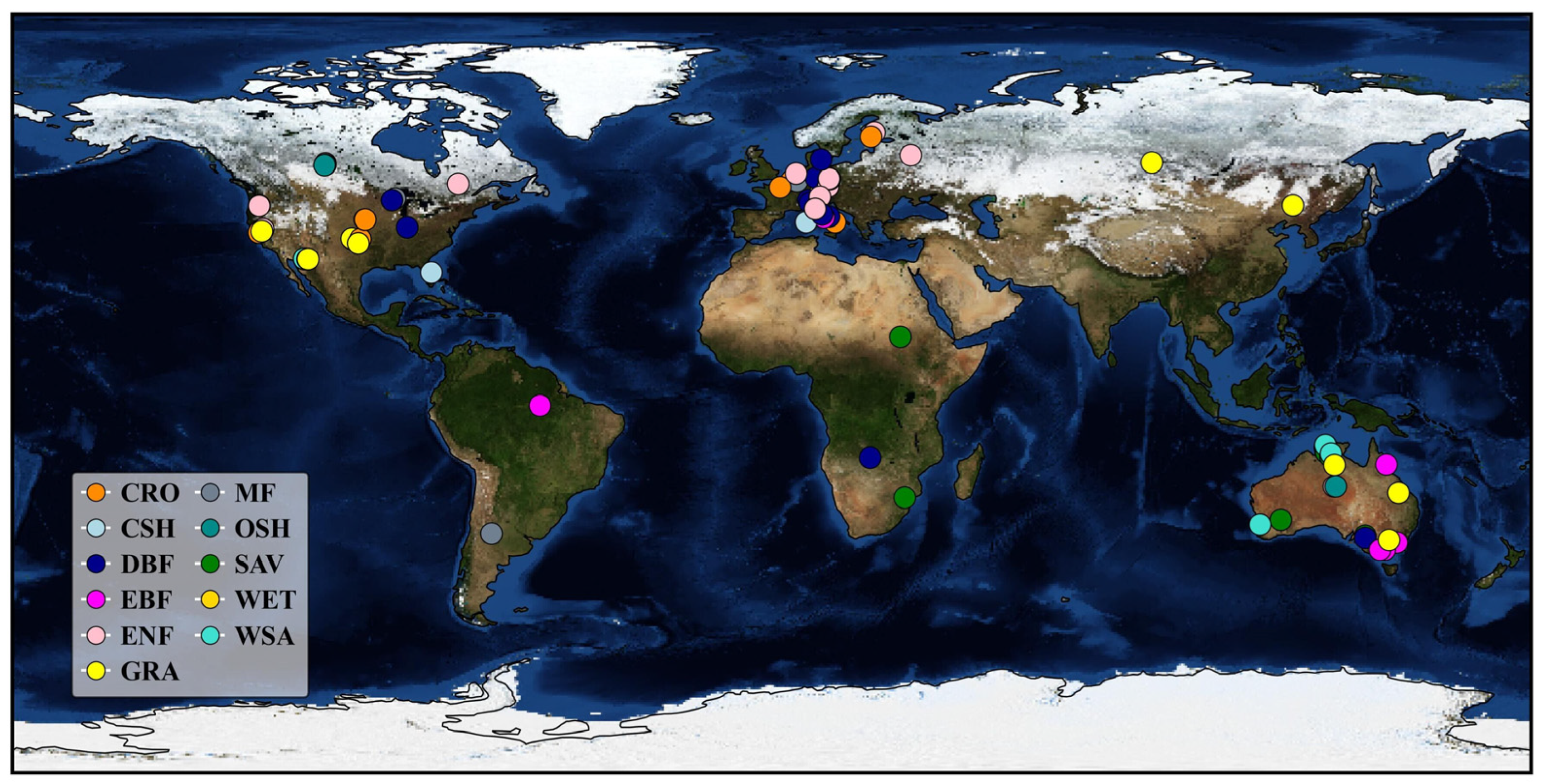
The hourly/half-hourly eddy fluxes, as well as meteorological data from the FLUXNET 2015 dataset [33], were employed to validate the two-step ET partitioning methods in this study. The sites with more than two years of continuous measurements and available soil moisture data were selected. To eliminate the influence of interception evaporation (Ei), ET measurements on days with rainfall events were excluded. For model development, only high-quality eddy flux data were retained for analysis. Eighty-five flux sites were selected in this study (Figure 2, Table S1), which cover evergreen needleleaf forests (ENF, 17 sites), evergreen broadleaf forests (EBF, 6 sites), deciduous broadleaf forests (DBF, 12 sites), mixed forests (MF, 3 sites), closed shrublands (CSH, 2 sites), open shrublands (OSH, 3 sites), savannas (SAV, 6 sites), woody savannas (WAS, 6 sites), grasslands (GRA, 16 sites), permanent wetlands (WET, 1 site), and croplands (CRO, 13 sites).
Information on vegetation characteristics, including canopy height (hc), leaf area index (LAI), vegetation index (VI), and fractional vegetation cover (FVC), is required for ET partitioning. hc data were retrieved from Biological, Ancillary, Disturbance, and Metadata (BADM) files. LAI and normalized difference vegetation index (NDVI) were acquired from Moderate Resolution Imaging Spectroradiometer (MODIS) MCD15A2 8-day 500 m LAI products and MOD/MYD13Q1 16-day 250 m VI products, respectively. Low-quality NDVI and LAI data (the pixel reliability of the vegetation index larger than 1 and the quality control flag of LAI not equal to ‘000’) were removed, and remaining data gaps were filled using a spatiotemporal filtering approach [34]. FVC was estimated from NDVI. The pixels within a 1 km × 1 km area surrounding the EC sites were used to match the eddy flux measurements. The original 8-day LAI and 16-day NDVI data were linearly interpolated to a daily scale.
F V C = N D V I N D V I s N D V I v N D V I s 2
where NDVIs and NDVIv denote the NDVI values of soil and vegetation. The value of the two thresholds is set by referring to Wu et al. [35] and is presented in Table S2.

2.2. Extraction of Pure E and T from Long-Term ET Measurements

A critical step in the two-step strategy is the extraction of pure E and pure T samples from ET measurements. The pure E typically occurs under bare-soil conditions or in the absence of active vegetation. In this study, pure E was identified using a threshold for fractional vegetation cover (FVC), with a site-specific threshold of 0.05, which balances the available sample size and quality of the E signal. In contrast, identifying pure T is more complex, as E tends to occur whenever soil moisture is available. Zhou et al. [29] used the 95th percentile of daily GPP to detect the T period. In contrast, Nelson et al. [30] proposed a more stringent set of criteria, focusing on the growing season under dry soil surface conditions. In this study, the filter of Nelson et al. [30] was adopted to detect pure T periods. The detailed rules include (1) half-hourly/hourly GPP > 0.05 μmol C m−2 s−1; (2) daily GPP > 0.5 g C m−2 day−1; (3) air temperature > 5 °C; (4) incoming solar radiation > 0 W m−2; (5) conservative surface wetness index (CSWI) <−0.5 mm.
C S W I = max S t , min P t , S max
S t = min S t 1 + P t E T t , S max
where St is the surface water storage (mm); Pt is the precipitation at time t, and Smax is the maximum allowable storage and is set to 5 mm [30,31]. The filled ET observations were used to generate a continuous CSWI.

2.3. Two-Source ET Models

Once pure E and T samples were obtained, the corresponding sub-models were calibrated separately. This study evaluated the two-step strategy within three classical two-source ET model frameworks: the Shuttleworth–Wallace (SW) model, the Priestley–Taylor Jet Propulsion Laboratory (PT-JPL) model, and the FAO-56 dual crop coefficient model (FAO56-DK). All three methods rely on routinely available meteorological, vegetation, and soil variables. Another widely used two-source model, thermal-based energy balance models, such as the two-source energy balance (TSEB) model [36], requires high-quality, continuous land surface temperature (LST) data as a primary driver, which is not available in this study. Therefore, thermal-based two-source models were not included in this evaluation.

2.3.1. SW Model

The formulation of the SW model is expressed as follows:
λ E T = λ T + λ E = C c P M c + C s P M s
P M c = Δ A + ρ a c p e s e a Δ r a c A s / r a a + r a s Δ + γ 1 + r s c / r a a + r a c
P M s = Δ A + ρ c p e s e a Δ r a s A A s / r a a + r a s Δ + γ 1 + r s s / r a a + r a s
C c = 1 + R c R a R s R c + R a 1
C s = 1 + R s R a R c R s + R a 1
R a = Δ + γ r a a
R s s = Δ + γ r a s + γ r s s
R c = Δ + γ r a c + γ r s c
A = R n G
A s = R n e k L A I G
where λ is the latent heat of vaporization; PMc and PMs denote the closed vegetation and bare soil latent heat fluxes (W m−2), respectively; Cc and Cs denote the canopy and soil resistance coefficients (unitless), respectively; Δ is the slope of the saturation vapor pressure curve (kPa K−1); γ is the humidity constant; ρa is the air density (kg m−3); cp is the constant pressure-specific heat (J kg−1); r a a , r a c and r a s denote the aerodynamic resistance; vegetation boundary layer resistance, and the soil boundary layer resistance, respectively (s m−1); r s s and r s c denote the soil surface resistance and vegetation canopy resistance, respectively (s m−1); A and As denote the available energy for the canopy and soil layer (W m−2), respectively; Rn is the net radiation (W m−2); G is the ground heat flux (W m−2); k is the light extinction coefficient (unitless); LAI is the leaf area index. The equations for the resistances are shown as follows:
r a a = 1 κ u * ln z d h c d + h c n K h e n 1 z 0 + d h c 1
r a s = h c e n n K h e n z 0 h c e n z 0 + d h c
n = 2.5 ,   h c < 1 0.194 h c + 2.306 , 4.25 ,   h c > 10   1 < h c < 10
K h = κ u * h c d
u * = κ u ln z d z 0
r a c = 100 n w u h 0.5 1 e n 2 1 2 L A I
r s c = 1 g 0 L A I + a 1 G P P R h / C a × 1.6 × 0.0224
r s s = b 1 θ s θ b 2 + b 3
where κ is von Karman constant (0.40); u* is the friction velocity (m s−1); z is the measurement height of wind speed (m); d is the zero-plane displacement (m); hc is the canopy height (m); z0 is the roughness length (m); n is the extinction coefficient of eddy diffusion (unitless); Kh is the turbulence attenuation coefficient at the top of the canopy; w is the characteristic leaf width (m); uh is the wind speed at the top of canopy (m s−1); Rh is relative humidity; GPP is the gross primary production (μmol m−2 s−1); Ca is the ambient CO2 concentration (μmol mol−1); θ is the surface soil moisture; θs is the saturated soil moisture; g0, a1, b1, b2, b3 denote the coefficients, respectively.

2.3.2. PT-JPL Model

The PT-JPL model is one of the most widely used two-source models based on the Priestley–Taylor formulation. The original PT-JPL divides ET into soil evaporation, plant transpiration, and canopy interception evaporation. Since canopy interception evaporation was not considered in this study, a modified version of the PT-JPL model [37] was adopted.
λ T = f G f T f M α Δ Δ + γ R n e k L A I
λ E = f s m α Δ Δ + γ 1 e k L A I R n G
f G = f A P A R f I P A R = m 1 N D V I n 1 m 2 N D V I n 2
f T = e T a T o p t T o p t 2
f M = f A P R A f A P R A , max
f S M = R h V P D / β
where α is the PT coefficient of 1.26 (unitless); fG, fT, fM, and fSM denote the green canopy fraction, plant temperature constraint, plant moisture constraint, and soil moisture constraint, respectively; fAPRA is the fraction of PAR absorbed by green vegetation cover; fIPAR is the fraction of PAR intercepted by the canopy plant; Topt is the optimum plant growth temperature (°C); β is the relative sensitivity to VPD. Previous studies set the values of m1, n1, m2, n2, and β as 1.16, 0.14, 1.0, 0.05, and 1 [37], and defined Topt as the Ta at max PARfAPRATa/VPD [38]. This study treated the six parameters as adjustable coefficients.

2.3.3. FAO-56 Dual Crop Coefficient Model (FAO56-DK)

The FAO56-DK method was originally designed for the calculation of crop evapotranspiration. This study extends the FAO56-DK method to other ecosystems. The dual crop coefficient model retrieves the actual evapotranspiration from reference evapotranspiration (E0) using the crop coefficient. The half-hourly ET0 was calculated as follows:
E T 0 = 0.408 Δ R n G + γ c n T a + 273 u V P D Δ + γ 1 + c d u
where for short vegetation, cn is set to 37 and cd equals 0.24 when Rn > 0 and 0.96 when Rn < 0; for tall vegetation, cn is 66 and cd is 1.7 when Rn > 0 and 0.25 when Rn < 0 [39]. This study employed the cn and cd of short vegetation for GRA and those of tall vegetation for other ecosystems.
T = K s K c b E T 0
E = K e E T 0
K c b = K c b , min + K c c K c b , f u l l K c b , min
K c c = 1 e k L A I
K e = K r K c , max K c b f e w K c , max
where Kcb is the basal crop coefficient; Ks is the water stress coefficient; Ke is the soil evaporation coefficient; Kcb, min and Kcb, full denote the minimum basal crop coefficient for bare soil and the basal crop coefficient when the crop has nearly full ground cover, respectively; Kcc is the canopy cover coefficient and is calculated using LAI; k is the canopy extinction coefficient and is set to 0.5; Kr is the evaporative reduction coefficient; Kc, max is the maximum value of the crop coefficient; few is the fraction of soil surface and is calculated as 1 − FVC. In the original FAO56-DK method, the Ks and Kr are calculated using the available soil water in the root zone and topsoil layer, respectively. However, many flux sites in the FLUXNET2015 dataset only provide one-layer soil moisture observations, with the measurement depth unspecified. Therefore, this study used one-layer soil moisture to estimate Kr and Ks.
K s = θ θ w 1 p θ s θ w
K r = θ 0.5 θ w θ s θ w
where p is the fraction of total available soil water that vegetation can extract from the root zone without experiencing water stress and is set to 0.45 [40]; θs and θw denote the saturated water content and wilt point. In addition, the original FAO56-DK model incorporates the effects of wind speed, relative humidity, and canopy height on Kcb,full. However, this correction is empirical and specifically tailored for the cropland ecosystem. Therefore, it was not applied in this study. Instead, Kcb,min, Kcb,full, and Kcmax were treated as adjustable parameters.
In both the SW and FAO56-DK models, the soil parameters θs and θw are required. Due to the absence of site-specific soil property information, θs and θw were empirically estimated based on the approach of Hu [41]. Specifically, θs and θw were defined as the maximum θ + 0.1 and the minimum θ − 0.1 (θw > 0), respectively.

2.4. Benchmark Approach for ET Partitions

This study selected the Nelson et al. method [30] (hereafter Nelson2018) to partition ET into E and T. Nelson2018 has been evaluated across multiple FLUXNET sites. Independent assessments have demonstrated that transpiration (T) estimates derived from the Nelson framework show strong agreement with sap flow measurements, with an average correlation coefficient of approximately 0.81, as well as with other established partitioning methods [31]. This method uses water use efficiency (WUE) to partition ET. ET observations are first filtered to identify periods when T dominates. A data-driven algorithm, random forest, is then used to construct a WUE model, which is subsequently applied to estimate T from GPP.
W U E = R F X t
T = G P P W U E
where RF is the random forest algorithm; Xt is the input feature set of the random forest algorithm, including incoming radiation (Rg), air temperature (Ta), relative humidity (RH), wind speed (u); four derived variables: the derivative of a Gaussian-filtered GPP (GPP′), the Rg-normalized diurnal centroid of ET ( C E T * ), the diurnal water: carbon index (DWCI), and conservative surface wetness index (CSWI); as well as daily potential radiation (Rgpot,daily), the derivative of daily potential radiation (Rgpot,daily′), and year. Details of these variables are provided in Nelson et al. [30] and the Supplementary Material Text S1.

2.5. Parameter Calibration and Accuracy Metrics

The adjustable parameters in all three two-source models were calibrated using the Differential Evolution Adaptive Metropolis (DREAM) algorithm [42]. The prior ranges of g0, a1, b1, b2, b3 in the SW model were set to 5–40, 0.001–0.1, 1–5, 1–5, 10–1000, respectively [25,26,40]. The prior ranges of m1, n1, m2, n2, β, Topt in the PT-JPL model were set to 1–1.5, 0–0.5, 1–1.5, 0–0.5, 0.5–2, 20–40, respectively [37,38]. For the FAO-DK model, three adjustable parameters exhibit an inherent magnitude ordering, namely, Kcb,min < Kcb,full, and Kcb,min < Kc,max. To enforce these constraints, the prior ranges of Kcb,min, Kcb,fullKcb,min, Kc,maxKcb,min were set to 0–1, 0–5, 0–5, respectively [43,44]. The DREAM algorithm was configured with 10 Markov chains and a maximum of 30,000 model evaluations. Latin Hypercube Sampling was used for prior sampling, and convergence was assessed using the Gelman–Rubin statistic. For each site, available observations were randomly divided into calibration and validation subsets at a 50-50% ratio. All parameters were estimated exclusively using the calibration dataset. The optimized parameter set obtained from calibration was then held fixed and directly applied to the validation dataset to assess model generalization performance. No additional calibration or parameter updating was performed during validation.
The performance of the ET partitioning strategies was evaluated across all sites. Three metrics, including correlation coefficient (R), coefficient of determination (R2), and root mean square error (RMSE), were employed to evaluate the accuracy of ET and its components.
R = i = 1 n o i o ¯ s i s ¯ i = 1 n o i o ¯ 2 s i s ¯ 2
R M S E = 1 n i = 1 n o i s i 2
R 2 = 1 i = 1 n o i s i 2 i = 1 n o i o ¯ 2
where oi and o ¯ denote the observation sample and mean observation value, respectively; si and s ¯ denote the estimation sample and the mean estimation value, respectively.

3. Results

3.1. Data Quality and Energy Balance Closure Analysis

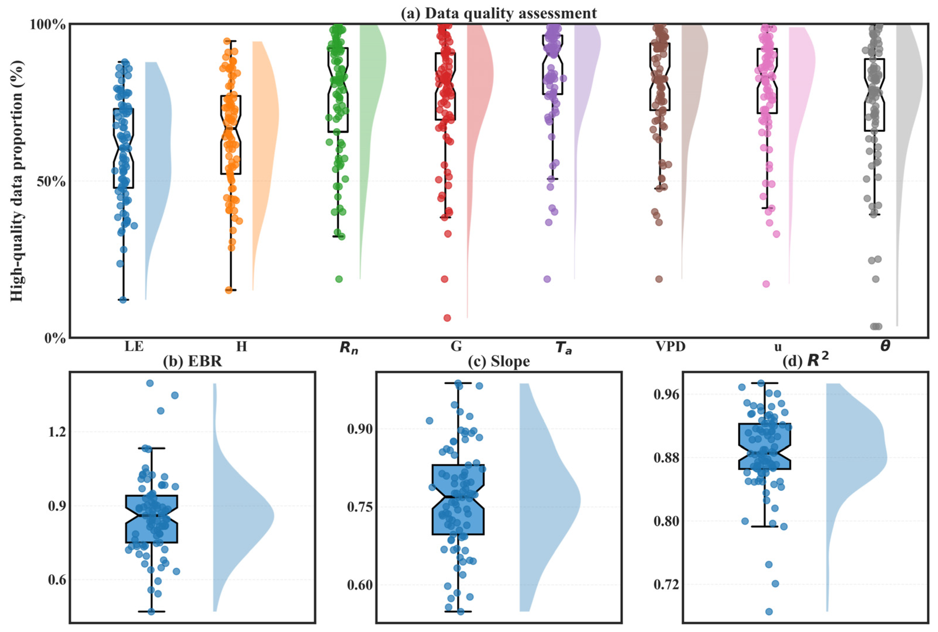
Figure 3 presents the data quality assessment and energy balance closure analysis across all sites. As shown in Figure 3a, the proportion of high-quality data is consistently high for most variables. The median proportion of high-quality data ranges approximately from 60% to 90%, with Rn, Ta, VPD, u, and θ generally exceeding 80%. In contrast, LE, H, and G exhibit relatively lower medians and greater variability.
Energy balance closure performance was evaluated using three complementary metrics: the energy balance ratio (EBR), defined as the ratio of the sum of latent and sensible heat fluxes (LE + H) to the available energy (RnG); the regression slope between LE + H and RnG; and the coefficient of determination (R2) for this regression. The EBR exhibits a median value of approximately 0.85. Most sites fall within the range of 0.75–0.95. A few sites display EBR values exceeding 1 or below 0.6. The regression slope between H + LE and RnG is generally close to unity, with a central tendency around 0.75–0.80. The relatively narrow interquartile range suggests consistent proportionality between measured and available energy across sites. The coefficient of determination (R2) is consistently high, with median values around 0.88–0.90. This indicates strong linear coupling between H + LE and Rn − G.
Overall, the dataset demonstrates sufficient data quality and reasonably consistent energy balance performance, supporting the reliability of the data for subsequent ET partitioning analyses.

3.2. Distribution of Pure Soil Evaporation and Plant Transpiration

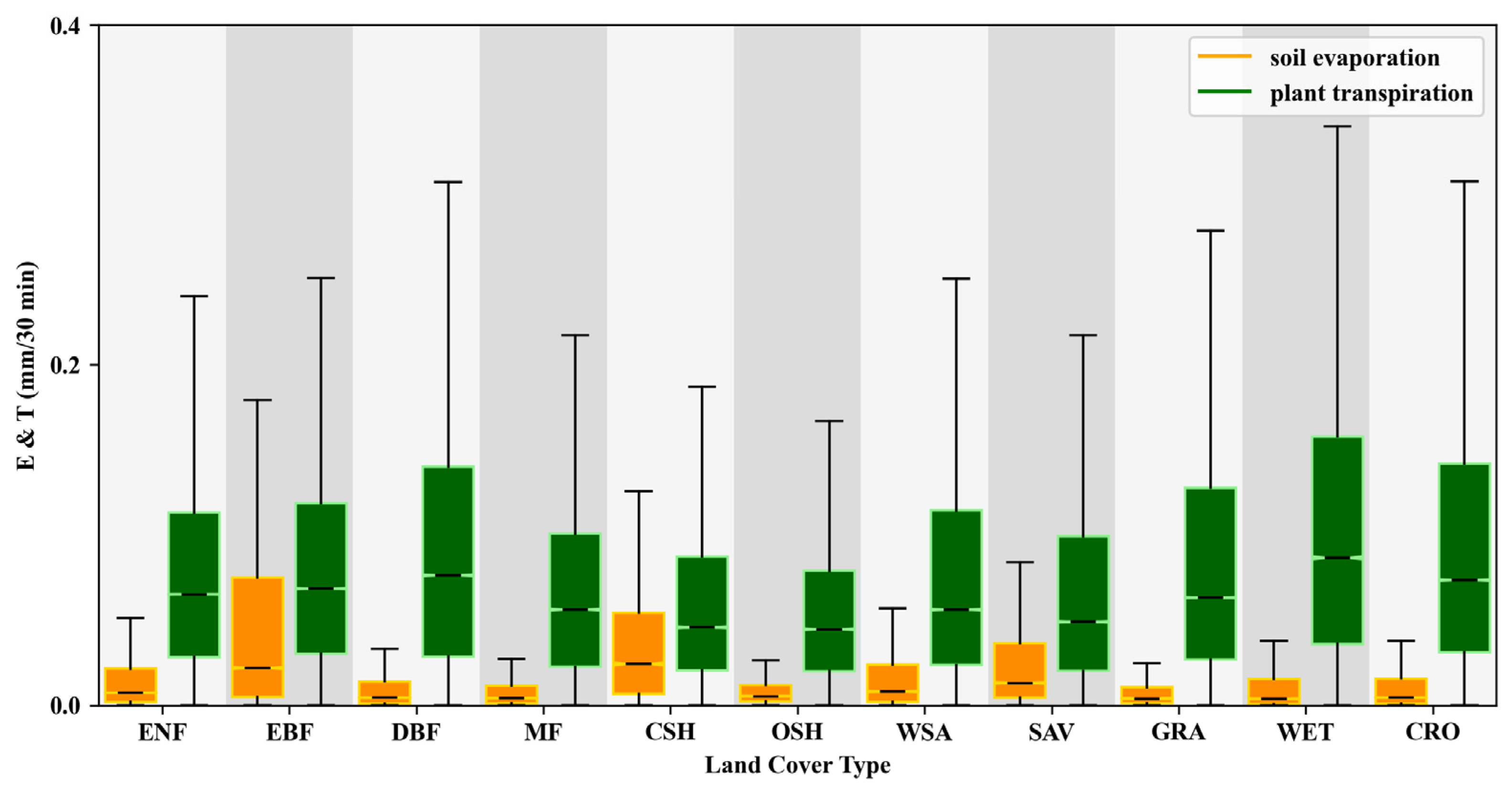
Figure 4 illustrates the distribution of pure soil evaporation and plant transpiration samples across different ecosystems. In most ecosystems, pure E remains relatively low compared to pure T. Notable exceptions include EBF and CSH, where E shows relatively higher median values. Across all ecosystems, the median values of pure E range from approximately 0.004 to 0.024 mm per half hour, while those of pure T are substantially higher, ranging from 0.044 to 0.086 mm per half hour. The highest median T is observed in WET, followed by CRO and ENF, while lower values appear in CSH and OSH. Variability is generally greater for pure T than for pure E. The dynamic amplitude (defined as the difference between the 75th and 25th percentiles, corresponding to the height of the box in the figure) of pure E varies from 0.01 to 0.07 mm per half hour, with the largest spread observed in EBF and CSH. In comparison, the dynamic amplitude of pure T is about 0.1 mm per half hour in most ecosystems, with the widest spread occurring in WET and CRO. The core hypothesis of this study is the existence of quasi-isolated pure E and pure T samples within long-term ET observations. The markedly different magnitudes of E and T support the reliability of this hypothesis.

3.3. Performance of ET Partitioning Strategies

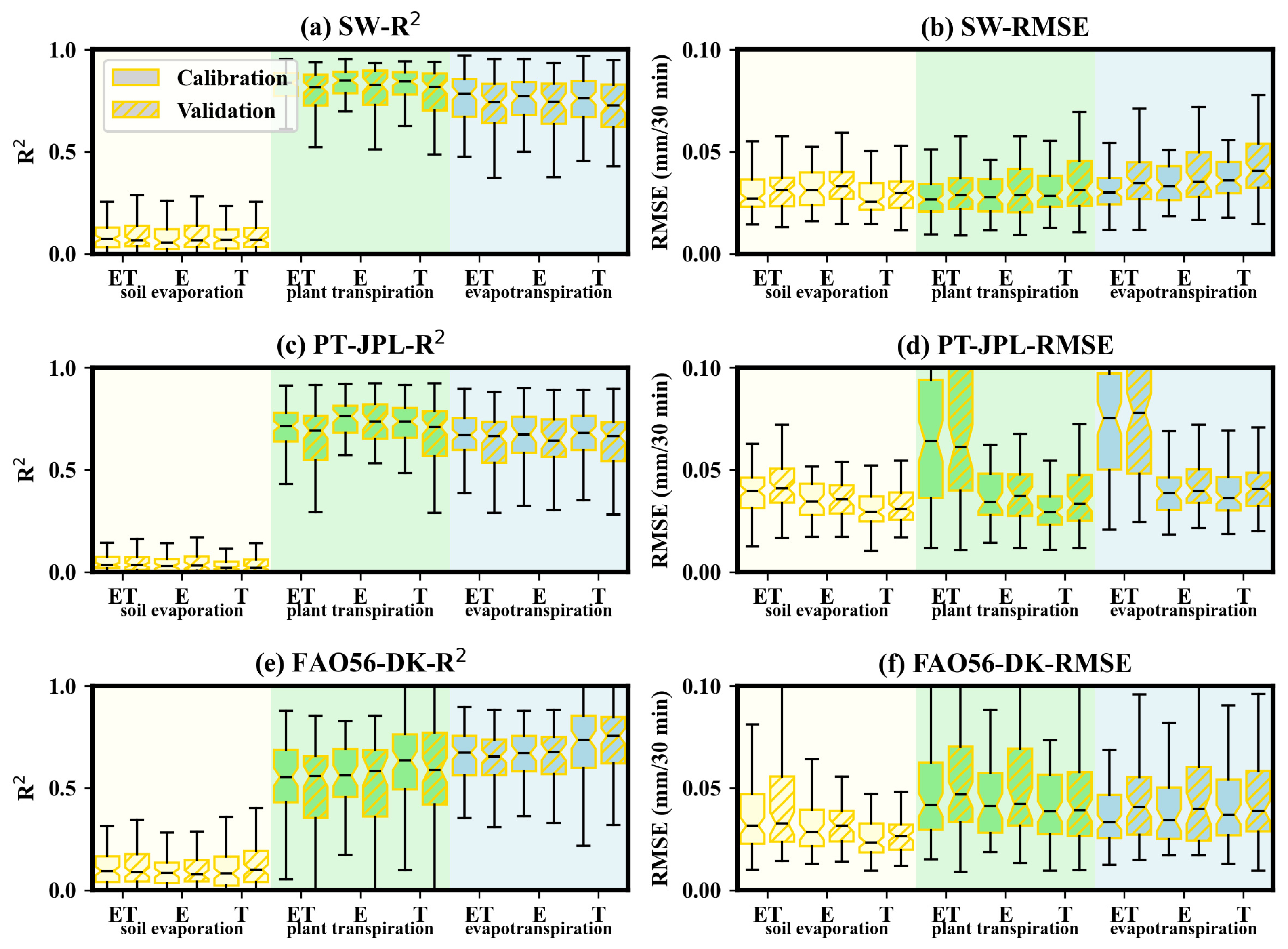
Figure 5 compares the accuracy of ET and its components across different ET partitioning strategies and two-source model frameworks. The accuracy is evaluated using the coefficient of determination (R2) and root mean square error (RMSE). Each box shows the distribution of accuracy metrics across sites. Under the SW model, the two-step strategies exhibit no evident advantage over the one-step strategy. The one-step strategy yields median R2 values of 0.07, 0.81, and 0.74, and median RMSEs of 0.031, 0.028, and 0.034 mm 30 min−1 for E, T, and ET, respectively. The two-step strategies achieve comparable accuracies. Specifically, the T-based two-step strategy shows slightly higher RMSE in ET estimates. In contrast, under the PT-JPL and FAO56-DK model frameworks, the two-step strategies deliver notably improved performance. Under the PT-JPL framework, the one-step strategy produces E estimates with a median R2 value of 0.04 and a median RMSE of 0.04 mm/30 min, T estimates with a median R2 value of 0.68 and a median RMSE of 0.06 mm/30 min, and ET estimates with a median R2 value of 0.66 and a median RMSE of 0.078 mm/30 min, respectively. By contrast, the two-step strategies substantially reduce the RMSE of E, T, and ET estimates to 0.03, 0.03, and 0.04 mm/30 min, respectively. Under the FAO56-DK framework, improvements are most evident for the T-based two-step strategy. The one-step strategy and the E-based two-step strategy yield E estimates with R2 of 0.08–0.09 and RMSE of 0.031 mm/30 min, T estimates with R2 of 0.55–0.58 and RMSE of 0.042–0.046 mm/30 min, and ET estimates with R2 of 0.65–0.67 and RMSE of 0.04 mm/30 min, respectively. By contrast, the T-based two-step strategy increases R2 of E, T, and ET estimates to 0.10, 0.65, and 0.75, respectively, and decreases the RMSE of E, T, and ET estimates to 0.026, 0.039, and 0.038 mm/30 min, respectively.
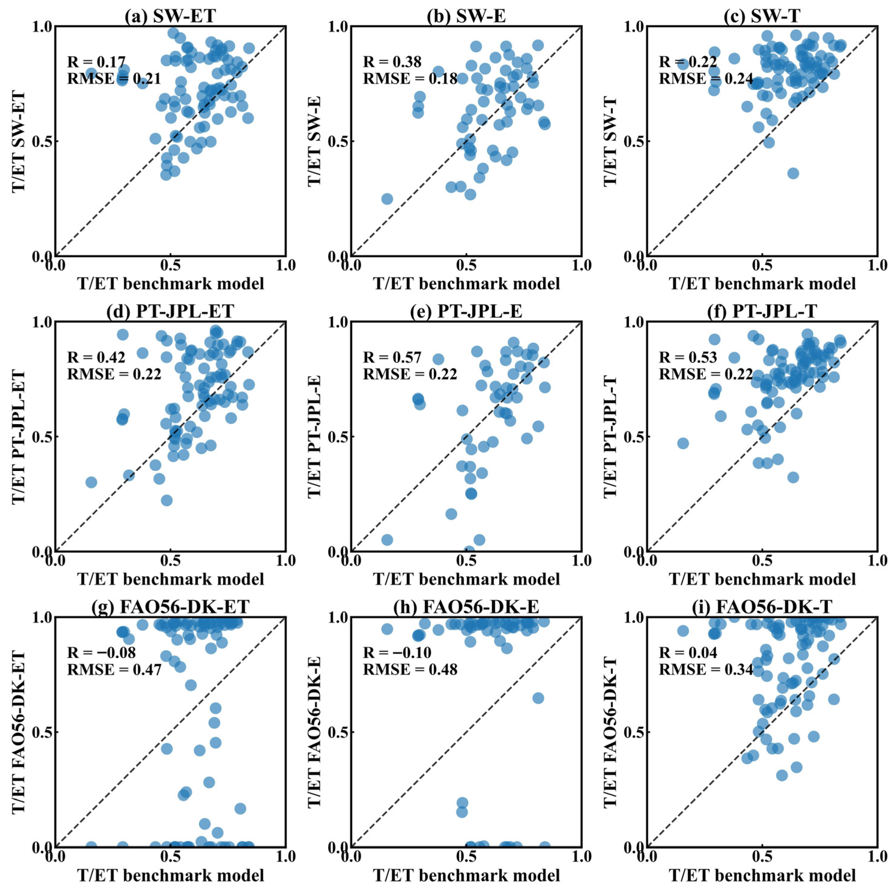
Figure 6 further evaluates the performance of two-step strategies across different two-source models in terms of the mean T/ET for each site (the ratio of accumulated T to accumulated ET). The accuracy is evaluated using the correlation coefficient (R) and root mean square error (RMSE). Overall, the two-step strategy generally improves the consistency between benchmark models and two-source models. When calibrating two-source models using all ET observations, the FAO56-DK model shows weak agreement with the benchmark models, yielding T/ET values close to 1 and R values near 0. In contrast, the SW and PT-JPL models exhibited moderate correlations with the benchmarks, with R ranging from 0.17 to 0.42 and RMSE values of 0.21 and 0.22. When using pure E to calibrate E-related parameters in the first step, the SW and PT-JPL models generated results closer to those of the benchmark model, with R increasing to 0.38 and 0.28, and RMSE decreasing to 0.18 and 0.22. However, for the FAO56-DK model, this strategy fails to improve ET partitioning performance, and T/ET remains close to 1. When using pure T to calibrate plant transpiration-related parameters in the first step, a slight improvement of ET partitioning can be observed in the SW and PT-JPL models. However, for the FAO56-DK model, this strategy led to a notable enhancement in performance, with RMSE decreasing to 0.34. These results highlight the substantial value of incorporating pure E and T information into ET partitioning. Moreover, the effectiveness of using pure samples varies depending on the specific two-source model framework employed.

3.4. Relation of ET Partitioning to Leaf Area Index and Soil Moisture

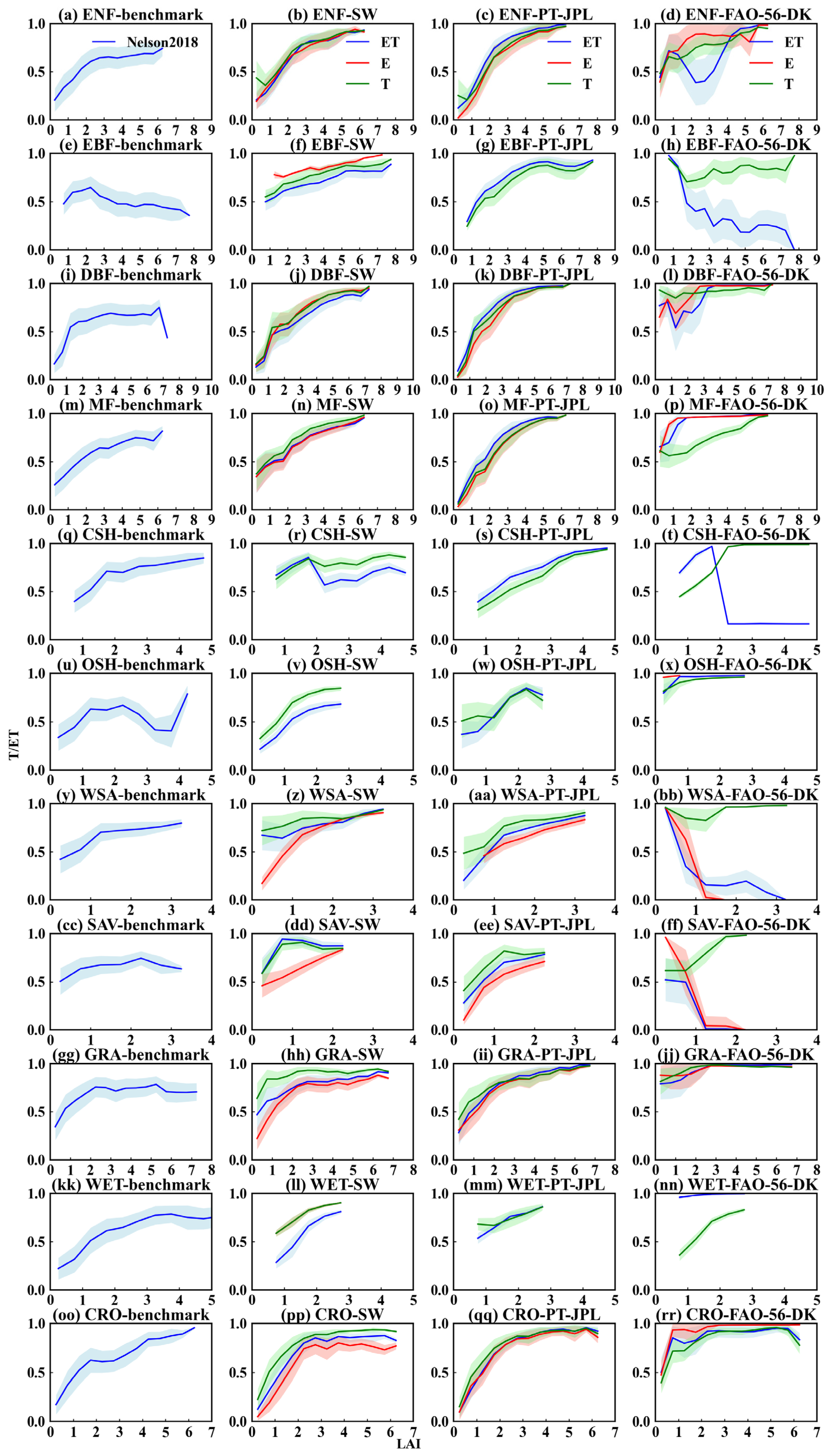
A positive relationship between T/ET and LAI has been widely reported in the literature. Figure 7 further assesses whether the modeled ET partitioning preserves this fundamental biophysical relationship. The solid lines and shaded regions depict the mean and standard deviation of daily T/ET within an LAI interval (0.5 LAI units). It can be seen that all ET partitioning algorithms generally capture the expected positive relationship between T/ET and LAI. The benchmark model exhibits a consistent increase in T/ET with LAI across most ecosystems, although deviations from this pattern are observed. In EBF, the benchmark model shows relatively stable T/ET values regardless of LAI. In OSH, the T/ET-LAI relationship fluctuates markedly. In most cases, one-step and two-step strategies produce a consistent T/ET-LAI relationship. Notably, the SW model and PT-JPL models yield a more stable positive relationship between T/ET and LAI. This indicates that the incorporation of physical constraints helps preserve the underlying biological relationship between T/ET and LAI. However, some exceptional results still exist. For example, the SW model produces a relatively stable T/ET-LAI relationship in CSH, and the PT-JPL model generates a decreasing trend of T/ET when using the pure T-based two-stage strategy. In contrast, the FAO56-DK model displays a more irregular relationship. When using the one-step strategy, T/ET values exhibit strong variability across LAI levels. By contrast, the pure T-based two-stage strategy yields a more stable increasing trend in most ecosystems. An exception is observed in EBF, where this approach unexpectedly produces a decreasing T/ET trend with increasing LAI.
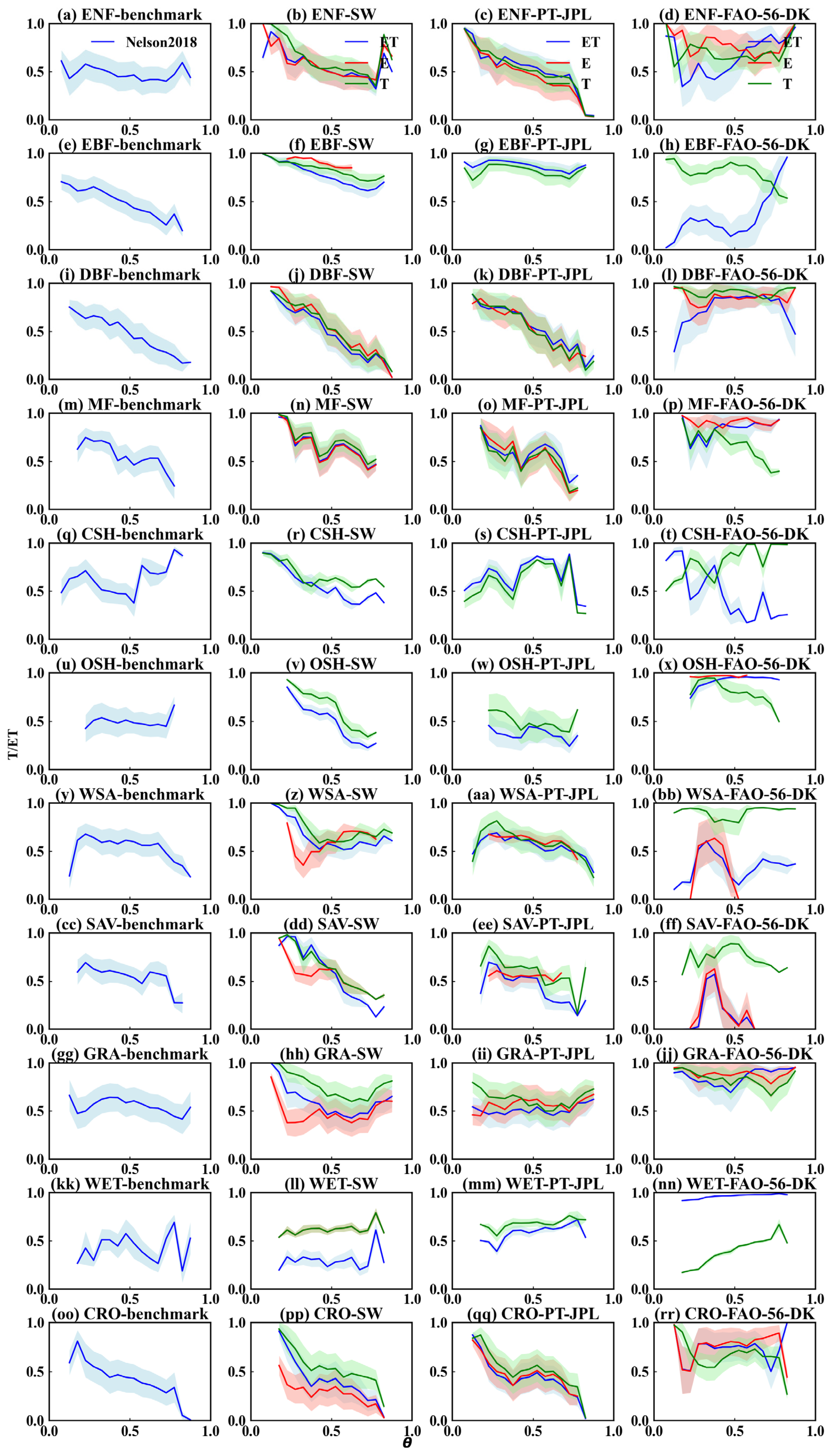
Soil moisture is also a key factor for regulating ET partitioning [44]. Figure 8 presents the relationship between soil moisture and T/ET under different ET partitioning strategies. It should be noted that soil moisture was normalized by θs and θw in Figure 7. It can be seen that the pattern of soil moisture–T/ET varies significantly across ecosystems and models. In many cases, a negative relationship between soil moisture and T/ET is evident, though notable exceptions also emerge. Three benchmark models displayed a relatively stable soil moisture–T/ET relationship in CRO, and an increasing trend in CSH. The SW model generally presents a decreasing trend of T/ET with increasing soil moisture across most ecosystems, with the exception of WET. Interestingly, the PT-JPL model, which does not explicitly incorporate soil moisture as an input, also retains a decreasing trend in ENF, DBF, SAV, and CRO. This suggests that vapor pressure deficit, which is included in the model, may serve as an effective proxy for soil moisture. However, the PT-JPL model yields a relatively stable soil moisture–T/ET relationship in EBF, OSH, and GRA. In MF, the one-step strategy results in a decreasing trend, whereas the two-step strategies based on pure E and pure T produce relatively stable patterns. In CSH, the soil moisture–T/ET relationship appears to plateau at moderate soil moisture levels (about 0.5), indicating a threshold beyond which further increases in soil moisture have little effect on ET partitioning. In contrast, the FAO56-DK model exhibits a highly irregular soil moisture–T/ET relationship, with no clear or consistent trend across ecosystems.

4. Discussion

4.1. How Does Pure E and T Information Influence ET Partitioning

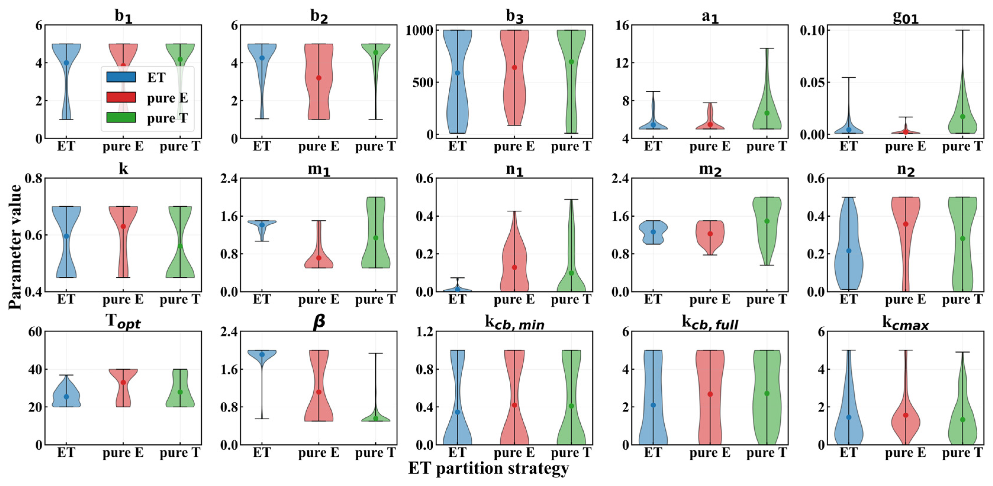
The intention of the two-step strategy is to use the pure E and T observations to independently constrain the soil evaporation and plant transpiration sub-models. Figure 9 displays the parameter value distribution of three two-source models under the one-step and two-step strategies. In the SW model, pure E observations typically decrease the value of b1 and b2, and pure T observations typically increase both a1 and g01. Accordingly, pure E decreases soil surface resistance and soil evaporation, while pure T slightly increases stomatal conductance and plant transpiration. Some previous studies have pointed out that the SW model typically underestimates E [45]. The pure E-based two-step strategy places greater emphasis on improving the E component, thereby mitigating this underestimation. In the PT-JPL model, pure E tends to decrease m1 and increase n2, while pure T tends to increase m1 and m2. Both pure E and T information decrease the soil moisture stress-related parameter β. These parameter shifts suggest that pure E observations enhance the soil evaporation rate. In the FAO56-DK model, both pure E and T information typically lead to higher Kcb,full, while their influence on Kcb,min and Kcmax do not exhibit obvious trends. The crop coefficient is the critical parameter in the FAO56-DK model. Some recent studies, such as Pereira et al. [42] and Rallo et al. [43], comprehensively summarized the value of Kcb across different vegetation types, including vegetation crops, vine fruit crops, and trees, and showed that Kcb at the mid-season stage is typically less than 1.2. Pereira et al. [42] reported the maximum Kcb,mid value of 1.16. In contrast, this study shows that Kcb,full often exceeds 2. This inconsistent Kcb value is likely due to the variation of ecosystems.

4.2. How Different Two-Source Model Structures Influence ET Partitioning

This study evaluated the two-step strategy across three classical two-source ET models with different structures. The SW model explicitly represents micrometeorological and plant biophysical processes for soil evaporation and plant transpiration, particularly the coupled relationship between soil surface resistance and canopy resistance (Equations (7) and (8)). Consequently, it produced the most robust and consistent results, effectively capturing distinct and coherent patterns, including an increasing trend of T/ET with rising LAI and a decreasing trend of T/ET with increasing θ. The PT-JPL model partitions net radiation between soil and canopy components in a manner similar to the SW model, and further incorporates NDVI to quantify plant stress via biophysical constraints. It also produced relatively stable and consistent results across ecosystems. However, the relationship between soil evaporation and plant transpiration in this model is described more independently, as the constraint factors for soil evaporation and plant transpiration are weakly linked. Therefore, separate information on E and T can contribute to the improvement of ET component estimates. In contrast, the FAO56-DK model exhibited high variability. Within this framework, the formulations for soil evaporation and plant transpiration are tightly coupled. Notably, the soil evaporation equation includes key parameters for plant transpiration (Kr(KcmaxKcb)). As a result, the integration of pure T information exerts a disproportionately strong influence on model behavior. Moreover, the FAO56-DK model directly scales both soil evaporation and plant transpiration from reference evapotranspiration, and does not explicitly account for interactions between soil and canopy processes, such as net radiation partitioning and resistances along water transfer pathways. Therefore, compared to the more physically based SW and PT-JPL models, the FAO56-DK model shows limited capability in capturing the regulatory effects of environmental factors on ET partitioning.

4.3. Limitations

This study proposes a novel ET partitioning method—the two-step strategy. The method extracts pure E and T samples from long-term EC observations and employs this pure E and T information to constrain the corresponding submodules of two-source ET models. The results demonstrate that incorporating pure E and T observations can lead to more robust and physically consistent ET partitioning. Compared with the benchmark method of Nelson et al. [30], the two-step strategy has the advantage of avoiding additional empirical assumptions beyond those already embedded within the two-source model structures. However, the efficacy of the proposed two-step strategy is subject to several critical limitations that warrant a cautious interpretation of the results. First, a fundamental challenge lies in the conceptual assumptions behind the identification of “pure” samples. The use of low-CSWI and high-GPP periods for pure T samples and low-FVC periods for pure E samples serves as an operational and heuristic approximation rather than a literal state of physical isolation. If these filters fail to adequately sequester the influence of the opposing component, the resulting submodule constraints may inherit systematic biases. Second, substantial model uncertainty arises from uncertainties in the physical two-source models, specifically the uncertainty in parameters. The soil parameters (θw and θs) are empirically determined. The assumption of parameter time-invariance implicitly holds in this study. Current model structures often rely on static parameters derived from limited time windows, yet in reality, soil hydraulic properties can be altered by agricultural disturbances like tillage [46], while plant physiological traits evolve dynamically with phenology [47]. Applying these “quasi-isolated” parameters to long-term simulations may fail to capture essential seasonal shifts, potentially misrepresenting the T/ET ratio over broader scales. Finally, this study lacks direct observations of soil evaporation and plant transpiration for model validation. ET components derived from Nelson et al. [30] were adopted as the benchmark values in this study. There are other similar approaches to partitioning ET measurements, such as Zhou et al. [29] and Li et al. [48]. Substantial discrepancies among these methods increase uncertainty in model validation (Figures S5 and S6). Recently, an independent transpiration measurement dataset, SAPFLUXNET, has become available. However, significant discrepancies between sap flux-based transpiration and model-based transpiration can be found (Nelson et al., [31]; Figures S2 and S3). Future research should prioritize collecting more in situ observations of ET components to enable more comprehensive and rigorous model validation.

5. Conclusions

This study proposes a two-step strategy for ET partitioning. The approach first extracts pure E and T observations from long-term ET data and then uses these samples to constrain the corresponding submodules in two-source ET models. The two-step strategy is evaluated in three classical two-source models, including the SW model, the PT-JPL model, and the FAO56-DK model, and validated against the traditional ET partitioning algorithm from Nelson et al. [30].
Our results demonstrate that the two-step strategy improves the consistency of T/ET estimates with those from the benchmark models, compared to the traditional one-step calibration approach. These findings highlight the value of incorporating pure E and T observations to enhance the accuracy of the soil evaporation and plant transpiration submodules within two-source ET models. However, the effectiveness of pure E and T information varies across model frameworks. In the SW and PT-JPL models, both pure E and T information can contribute to improving ET partitioning accuracy. In contrast, in the FAO56-DK model, only pure T information helps to enhance ET partitioning accuracy. The main reason is that transpiration-related parameters influence the evaporation process.
Although this study lacks direct observational validation via lysimeters, sap flow systems, or isotopic techniques, which are rarely available at long-term ecosystem-scale flux sites, the proposed strategy demonstrates strong inter-methodological consistency. We conclude that the two-step approach offers a robust framework for improving the stability of ET partitioning in the absence of direct component measurements. Future research incorporating high-frequency, direct observations of E and T will be essential to further validate the physical accuracy of these findings and to refine the global applicability of this strategy for large-scale hydrological monitoring.

Supplementary Materials

The following supporting information can be downloaded at https://www.mdpi.com/article/10.3390/agronomy16050559/s1, Text S1: ET partitions methods; Figure S1: Accuracy of RF-based WUE model; Figure S2: Performance of one-step and two-step strategies for ET component estimation under different two-source model frameworks. The ET components is derived from method of Zhou et al. (2016) [29]. The light yellow, green, and blue backgrounds denote soil evaporation, plant transpiration, and total evapotranspiration, respectively. The labels “ET”, “E”, and “T” represent the one-step, E-based two-step, and T-based two-step strategies. Solid and hatched boxplots correspond to calibration and validation datasets, respectively; Figure S3: Performance of one-step and two-step strategies for ET component estimation under different two-source model frameworks. The ET components is derived from method of Li et al. (2019) [48]. The light yellow, green, and blue backgrounds denote soil evaporation, plant transpiration, and total evapotranspiration, respectively. The labels “ET”, “E”, and “T” represent the one-step, E-based two-step, and T-based two-step strategies. Solid and hatched boxplots correspond to calibration and validation datasets, respectively; Figure S4: The performance of ET partitioning algorithms from aspect of T/ET. Zhou2016, Nelson2018 and Li2019 denote methods of Zhou et al. (2016), Nelson et al. (2018) and Li et al. (2019) [29,30,48], respectively; Figure S5: The relationship between sap flux-based T and model-based T at NL-Loo site; Figure S6: The relationship between sap flux-based T and model-based T at RU-Fyo site; Table S1: The list of EC sites selected in this study; Table S2: The NDVI value of soil and vegetation for each site.

Author Contributions

Conceptualization, X.H. and X.D.; methodology, X.H., Z.H., L.S., L.L. and Y.J.; software, X.D.; validation, X.H.; formal analysis, X.D.; investigation, X.H.; resources, L.S.; data curation, X.H. and X.D.; writing—original draft preparation, X.H. and X.D.; writing—review and editing, Z.H. and L.S.; visualization, X.D.; supervision, Z.H.; project administration, L.S.; funding acquisition, X.H. All authors have read and agreed to the published version of the manuscript.

Funding

This work was supported by the Open Research Fund of State Key Laboratory of Efficient Utilization of Agricultural Water Resources (Grants No. SKLAWR-2024-07) and National Natural Science Foundation of China (Grants No. 52309058).

Data Availability Statement

The data presented in this study are available upon request from the corresponding author due to privacy considerations.

Acknowledgments

The authors gratefully acknowledge all of the researchers for their contributions to each flux site and the organizers of the FLUXNET database.

Conflicts of Interest

The authors declare no conflicts of interest.

References

  1. Qiu, R.; Katul, G.G.; Zhang, L.; Qin, S.; Jiang, X. The effects of changing environments, abiotic stresses, and management practices on cropland evapotranspiration: A review. Rev. Geophys. 2025, 63, e2024RG000858. [Google Scholar] [CrossRef]
  2. Fisher, J.B.; Melton, F.; Middleton, E.; Hain, C.; Anderson, M.; Allen, R.; Wood, E.F. The future of evapotranspiration: Global requirements for ecosystem functioning, carbon and climate feedbacks, agricultural management, and water resources. Water Resour. Res. 2017, 53, 2618–2626. [Google Scholar] [CrossRef]
  3. Li, C.; Han, J.; He, Y.; Shen, J.; Liu, Z.; Yang, H. Assessing global transpiration estimates: Insights from tree-scale sap flow analysis. J. Hydrol. 2024, 637, 131419. [Google Scholar] [CrossRef]
  4. Gentine, P.; Green, J.K.; Guérin, M.; Humphrey, V.; Seneviratne, S.I.; Zhang, Y.; Zhou, S. Coupling between the terrestrial carbon and water cycles-a review. Environ. Res. Lett. 2019, 14, 083003. [Google Scholar] [CrossRef]
  5. Or, D.; Lehmann, P.; Shahraeeni, E.; Shokri, N. Advances in soil evaporation physics—A review. Vadose Zone J. 2013, 12, 1–16. [Google Scholar] [CrossRef]
  6. Xiao, Q.; McPherson, E.G. Surface water storage capacity of twenty tree species in Davis, California. J. Environ. Qual. 2016, 45, 188–198. [Google Scholar] [CrossRef] [PubMed]
  7. Wang, L.; Caylor, K.K.; Villegas, J.C.; Barron-Gafford, G.A.; Breshears, D.D.; Huxman, T.E. Partitioning evapotranspiration across gradients of woody plant cover: Assessment of a stable isotope technique. Geophys. Res. Lett. 2010, 37, L09401. [Google Scholar] [CrossRef]
  8. Xiao, W.; Wei, Z.; Wen, X. Evapotranspiration partitioning at the ecosystem scale using the stable isotope method—A review. Agric. For. Meteorol. 2018, 263, 346–361. [Google Scholar] [CrossRef]
  9. Boast, C.W.; Roberston, T.M. A “micro-lysimeter” method for determining evaporation from bare soil: Description and laboratory evaluation. Soil Sci. Soc. Am. J. 1982, 46, 689–696. [Google Scholar] [CrossRef]
  10. Liu, C.; Zhang, X.; Zhang, Y. Determination of daily evaporation and evapotranspiration of winter wheat and maize by large-scale weighing lysimeter and micro-lysimeter. Agric. For. Meteorol. 2002, 30, 109–120. [Google Scholar] [CrossRef]
  11. Oren, R.; Phillips, N.; Katul, G.; Ewers, B.E.; Pataki, D.E. Scaling xylem sap flux and soil water balance and calculating variance: A method for partitioning water flux in forests. Ann. For. Sci. 1998, 55, 191–216. [Google Scholar] [CrossRef]
  12. Poyatos, R.; Granda, V.; Flo, V.; Adams, M.A.; Adorján, B.; Aguadé, D.; Aidar, M.P.M.; Allen, S.; Alvarado-Barrientos, M.S.; Anderson-Teixeira, K.J.; et al. Global transpiration data from sap flow measurements: The SAPFLUXNET database. Earth Syst. Sci. Data 2021, 13, 2607–2649. [Google Scholar] [CrossRef]
  13. Li, W.; Duveiller, G.; Wieneke, S.; Forkel, M.; Gentine, P.; Reichstein, M.; Niu, S.; Migliavacca, M.; Orth, R. Regulation of the global carbon and water cycles through vegetation structural and physiological dynamics. Environ. Res. Lett. 2024, 19, 073008. [Google Scholar] [CrossRef]
  14. Kool, D.; Agam, N.; Lazarovitch, N.; Heitman, J.L.; Sauer, T.J.; Ben-Gal, A. A review of approaches for evapotranspiration partitioning. Agric. For. Meteorol. 2014, 184, 56–70. [Google Scholar] [CrossRef]
  15. Wang, D.; Gao, G.; An, J.; Shao, Y.; Lv, Y.; Fu, B. Comparisons of three scaling up methods to estimate stand transpiration of a xerophytic shrub (Salix psammophila) in northern China. J. Hydrol. 2022, 608, 127593. [Google Scholar] [CrossRef]
  16. Williams, D.G.; Cable, W.; Hultine, K.; Hoedjes, J.C.B.; Yepez, E.A.; Simonneaux, V.; Er-Raki, S.; Boulet, G.; de Bruin, H.A.R.; Chehbouni, A.; et al. Evapotranspiration components determined by stable isotope, sap flow and eddy covariance techniques. Agric. For. Meteorol. 2004, 125, 241–258. [Google Scholar] [CrossRef]
  17. Rafi, Z.; Merlin, O.; Dantec, V.L.; Khabba, S.; Mordelet, P.; Er-Rask, S.; Amazirh, A.; Olivera-Guerra, L.; Hssaine, B.A.; Simonneaux, V.; et al. Partitioning evapotranspiration of a drip-irrigated wheat crop: Intercomparing eddy covariance-, sap flow-, lysimeter- and FAO-based methods. Agric. For. Meteorol. 2019, 265, 310–326. [Google Scholar] [CrossRef]
  18. Sun, X.; Wilcox, B.P.; Zou, C.B. Evapotranspiration partitioning in dryland ecosystems: A global meta-analysis of in situ studies. J. Hydrol. 2019, 576, 123–136. [Google Scholar] [CrossRef]
  19. Baldocchi, D.D. How eddy covariance flux measurements have contributed to our understanding of Global Change Biology. Glob. Change Biol. 2020, 26, 242–260. [Google Scholar] [CrossRef]
  20. Mu, Q.; Zhao, M.; Running, S.W. Improvements to a MODIS global terrestrial evapotranspiration algorithm. Remote Sens. Environ. 2011, 115, 1781–1800. [Google Scholar] [CrossRef]
  21. Yao, Y.; Liang, S.; Chen, J.; Liu, S.; Fisher, J.B.; Zhang, X.; Jia, K.; Zhao, X.; Qin, Q.; Zhao, B.; et al. MODIS-driven estimation of terrestrial latent heat flux in China based on a modified Priestley–Taylor algorithm. Agric. For. Meteorol. 2020, 171–172, 187–202. [Google Scholar] [CrossRef]
  22. Fisher, J.B.; Lee, B.; Purdy, A.J.; Halverson, G.H.; Dohlen, M.B.; Cawse-Nicholson, K.; Wang, A.; Anderson, R.G.; Aragon, B.; Arain, M.A.; et al. ECOSTRESS: NASA’s next generation mission to measure evapotranspiration from the international space station. Water Resour. Res. 2020, 56, e2019WR026058. [Google Scholar] [CrossRef]
  23. Anderson, R.G.; Alfieri, J.G.; Tirado-Corbalá, R.; Gartuning, J.; McKee, L.G.; Prueger, J.H.; Wang, D.; Ayars, J.E.; Kuatas, W.P. Assessing FAO-56 dual crop coefficients using eddy covariance flux partitioning. Agric. Water Manag. 2020, 179, 92–102. [Google Scholar] [CrossRef]
  24. Xue, K.; Song, L.; Xu, Y.; Liu, S.; Zhao, G.; Tao, S.; Magliulo, E.; Manco, A.; Liddell, M.; Wohlfahrt, G.; et al. Estimating ecosystem evaporation and transpiration using a soil moisture coupled two-source energy balance model across FLUXNET sites. Agric. For. Meteorol. 2020, 337, 109513. [Google Scholar] [CrossRef]
  25. Hu, Z.; Yu, G.; Zhou, Y.; Sun, X.; Li, Y.; Shi, P.; Wang, Y.; Song, X.; Zheng, Z.; Zhang, L.; et al. Partitioning of evapotranspiration and its controls in four grassland ecosystems: Application of a two-source model. Agric. For. Meteorol. 2009, 149, 1410–1420. [Google Scholar] [CrossRef]
  26. Chen, H.; Jiang, A.Z.; Huang, J.J.; Li, H.; McBean, E.; Singh, V.P.; Zhang, J.; Lan, Z.; Gao, J.; Zhou, Z. An enhanced shuttleworth-wallace model for simulation of evapotranspiration and its components. Agric. For. Meteorol. 2020, 313, 108769. [Google Scholar] [CrossRef]
  27. Zhu, Q.; Zhuang, Q. Parameterization and sensitivity analysis of a process-based terrestrial ecosystem model using adjoint method. J. Adv. Model. Earth Syst. 2020, 6, 315–331. [Google Scholar] [CrossRef]
  28. Song, Y.; Jin, L.; Zhu, G.; Ma, M. Parameter estimation for a simple two-source evapotranspiration model using Bayesian inference and its application to remotely sensed estimations of latent heat flux at the regional scale. Agric. For. Meteorol. 2016, 230–231, 20–32. [Google Scholar] [CrossRef]
  29. Zhou, S.; Yu, B.; Zhang, Y.; Huang, Y.; Wang, G. Partitioning evapotranspiration based on the concept of underlying water use efficiency. Water Resour. Res. 2016, 52, 1160–1175. [Google Scholar] [CrossRef]
  30. Nelson, J.A.; Carvalhais, N.; Cuntz, M.; Delpierre, N.; Knauer, J.; Ogée, J.; Jung, M. Coupling water and carbon fluxes to constrain estimates of transpiration: The TEA algorithm. J. Geophys. Res. Biogeosci. 2018, 123, 3617–3632. [Google Scholar] [CrossRef]
  31. Nelson, J.A.; Pérez-Priego, O.; Zhou, S. Ecosystem transpiration and evaporation: Insights from three water flux partitioning methods across FLUXNET sites. Glob. Change Biol. 2020, 26, 6916–6930. [Google Scholar] [CrossRef] [PubMed]
  32. Scott, R.L.; Knowles, J.F.; Nelson, J.A.; Gentine, P.; Li, X.; Barron-Gafford, G.; Bryant, R.; Biederman, J.A. Water availability impacts on evapotranspiration partitioning. Agric. For. Meteorol. 2021, 297, 108251. [Google Scholar] [CrossRef]
  33. Pastorello, G.; Trotta, C.; Canfora, E.; Chu, H.; Christianson, D.; Cheah, Y.W.; Poindexter, C.; Chen, J.; Elbashandy, A.; Humphrey, M.; et al. The FLUXNET2015 dataset and the ONEFlux processing pipeline for eddy covariance data. Sci. Data 2020, 7, 225. [Google Scholar] [CrossRef]
  34. Yuan, H.; Dai, Y.; Xiao, Z.; Ji, D.; Shangguan, W. Reprocessing the MODIS Leaf Area Index products for land surface and climate modelling. Remote Sens. Environ. 2011, 115, 1171–1187. [Google Scholar] [CrossRef]
  35. Wu, D.; Wu, H.; Zhao, X.; Zhou, T.; Tang, B.; Zhao, W.; Jia, K. Evaluation of spatiotemporal variations of global fractional vegetation cover based on GIMMS NDVI data from 1982 to 2011. Remote Sens. 2014, 6, 4217–4239. [Google Scholar] [CrossRef]
  36. Anderson, M.C.; Kustas, W.P.; Norman, J.M. A brief history of the thermal IR-based Two-Source Energy Balance (TSEB) model—Diagnosing evapotranspiration from plant to global scales. Agric. For. Meteorol. 2024, 350, 109951. [Google Scholar] [CrossRef]
  37. Zhang, L.; Marshall, M.; Nelson, A.; Vrieling, A. A global assessment of PT-JPL soil evaporation in agroecosystems with optical, thermal, and microwave satellite data. Agric. For. Meteorol. 2021, 306, 108455. [Google Scholar] [CrossRef]
  38. Purdy, A.J.; Fisher, J.B.; Goulden, M.L.; Colliander, A.; Halverson, G.; Tu, K.; Famiglietti, J.S. SMAP soil moisture improves global evapotranspiration. Remote Sens. Environ. 2018, 219, 1–14. [Google Scholar] [CrossRef]
  39. Walter, I.A.; Allen, R.G.; Elliott, R.; Itenfisu, D.; Brown, P.; Jensen, M.E.; Mecham, B.; Howell, T.A.; Snyder, R.; Eching, S.; et al. The ASCE Standardized Reference Evapotranspiration Equation; American Society of Civil Engineers: Reston, VA, USA, 2005. [Google Scholar]
  40. Gao, X.; Mei, X.; Zhang, J.; Cai, J.; Gu, F.; Hao, W.; Gong, D. Comparison of three modified models in evapotranspiration and its components over a rainfed spring maize cropland on the Loess Plateau, China. Agric. For. Meteorol. 2023, 330, 109322. [Google Scholar] [CrossRef]
  41. Laloy, E.; Vrugt, J.A. High-dimensional posterior exploration of hydrologic models using multiple-try DREAM(ZS) and high-performance computing. Water Resour. Res. 2012, 48, W01526. [Google Scholar] [CrossRef]
  42. Pereira, L.S.; Paredes, P.; López-Urrea, P.; Hunsaker, D.J.; Mota, M.; Shad, Z.M. Standard single and basal crop coefficients for vegetable crops, an update of FAO56 crop water requirements approach. Agric. Water Manag. 2021, 243, 106196. [Google Scholar] [CrossRef]
  43. Rallo, G.; Paço, T.A.; Paredes, P.; Puig-Sirera, À.; Massai, R.; Provenzano, G.; Pereira, L.S. Updated single and dual crop coefficients for tree and vine fruit crops. Agric. Water Manag. 2021, 250, 106645. [Google Scholar] [CrossRef]
  44. Sepaskhah, A.R.; Ilampour, S. Effects of soil moisture stress on evapotranspiration partitioning. Agric. Water Manag. 1995, 28, 311–323. [Google Scholar] [CrossRef]
  45. Zhao, P.; Li, S.; Li, F.; Du, T.; Tong, L.; Kang, S. Comparison of dual crop coefficient method and Shuttleworth–Wallace model in evapotranspiration partitioning in a vineyard of northwest China. Agric. Water Manag. 2015, 160, 41–56. [Google Scholar] [CrossRef]
  46. Steiner, J.L. Tillage and surface residue effects on evaporation from soils. Soil Sci. Soc. Am. J. 1989, 53, 911–916. [Google Scholar] [CrossRef]
  47. Forster, M.A.; Kim, T.D.H.; Kunz, S.; Abuseif, M.; Chulliparambil, V.R.; Srichandra, J.; Michael, R.N. Phenology and canopy conductance limit the accuracy of 20 evapotranspiration models in predicting transpiration. Agric. For. Meteorol. 2022, 315, 108824. [Google Scholar] [CrossRef]
  48. Li, X.; Gentine, P.; Lin, C.; Zhou, S.; Sun, Z.; Zheng, Y.; Liu, J.; Zheng, C. A simple and objective method to partition evapotranspiration into transpiration and evaporation at eddy-covariance sites. Agric. For. Meteorol. 2019, 265, 171–182. [Google Scholar] [CrossRef]
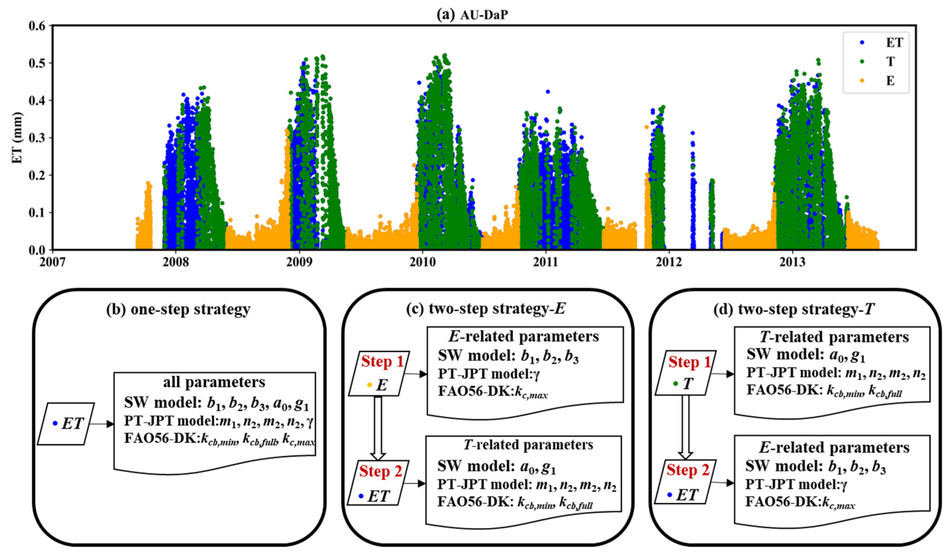
Figure 1. Flowchart of the ET partitioning strategies used in this study. (a) Illustration of pure E and T samples in the long-term ET observations; (b) the one-step strategy that uses all ET samples to calibrate both E-related and T-related parameters simultaneously; (c) the two-step strategy that uses pure E samples to calibrate E-related parameters in the first step and then uses the remaining ET samples to calibrate T-related parameters in the second step; (d) the two-step strategy that uses pure T samples to calibrate T-related parameters in the first step and then uses the remaining ET samples to calibrate E-related parameters in the second step.
Agronomy 16 00559 g001
Figure 2. Location of flux sites in this study.
Agronomy 16 00559 g002
Figure 3. Data quality and energy balance closure assessment across all sites. (a) Proportion of high-quality observations for each variable; (b) EBR of all sites; (c) regression slope of LE + H vs. Rn G; (d) coefficient of determination for LE + H vs. RnG regression line.
Agronomy 16 00559 g003
Figure 4. The distribution of pure soil evaporation and plant transpiration samples across different ecosystems.
Agronomy 16 00559 g004
Figure 5. Performance of one-step and two-step strategies for ET component estimates under different two-source model frameworks. The light yellow, green, and blue backgrounds denote soil evaporation, plant transpiration, and total evapotranspiration, respectively. The labels “ET”, “E”, and “T” represent the one-step, E-based two-step, and T-based two-step strategies. Solid and hatched boxplots correspond to calibration and validation datasets, respectively. Model performance under the SW, PT-JPL, and FAO56-DK frameworks was evaluated using data from 58, 47, and 56 sites.
Agronomy 16 00559 g005
Figure 6. The performance of ET partitioning algorithms in terms of T/ET.
Agronomy 16 00559 g006
Figure 7. The relationship between LAI and T/ET across different ecosystems within different ET partitioning frameworks.
Agronomy 16 00559 g007
Figure 8. The relationship between soil moisture (θ) and T/ET across different ecosystems within different ET partitioning frameworks.
Agronomy 16 00559 g008
Figure 9. The distribution of parameter values under one-step and two-step ET partitioning strategies. The central dot within each violin denotes the median parameter value across sites. The filled violin shapes represent the probability density distribution of each parameter across all sites. The vertical extent of each violin indicates the overall range of parameter values, while the width at a given value reflects the relative frequency of that value.
Agronomy 16 00559 g009
Disclaimer/Publisher’s Note: The statements, opinions and data contained in all publications are solely those of the individual author(s) and contributor(s) and not of MDPI and/or the editor(s). MDPI and/or the editor(s) disclaim responsibility for any injury to people or property resulting from any ideas, methods, instructions or products referred to in the content.