Article

First-Year Effects of Biochar, Biosolids, and Greenwaste on Tall Fescue Under Deficit Irrigation: Part I

by
Jaime Barros Silva Filho
1,*,
Jonathan Montgomery
2,
Marco Schiavon
3 and
Milton E. McGiffen, Jr.
4,*
1
Pacific Southwest Research Station, US Forest Service, United States Department of Agriculture (USDA), 4955 Canyon Crest Dr., Riverside, CA 92507, USA
2
Department of Biology, California State Polytechnic University at Humboldt, 1 Harpst Street, Arcata, CA 95521, USA
3
Agronomy Department, Fort Lauderdale Research and Education Center, University of Florida, Davie, FL 33314, USA
4
Department of Botany and Plant Sciences, University of California at Riverside, 900 University Avenue, Riverside, CA 92521, USA
*
Authors to whom correspondence should be addressed.
Agronomy 2026, 16(13), 1283; https://doi.org/10.3390/agronomy16131283
Submission received: 14 May 2026 / Revised: 18 June 2026 / Accepted: 1 July 2026 / Published: 3 July 2026

Abstract

As urban water scarcity intensifies, selecting soil amendments is critical for drought-stressed landscapes. This study evaluated biochar, biosolids, and greenwaste effects on canopy quality, soil moisture, nitrogen dynamics, and root architecture in tall fescue (Schedonorus arundinaceus) in the post-establishment year. Eight amendment treatments were assessed under two irrigation regimes (50% and 85% of reference evapotranspiration [ET0]) in a split-split-plot arrangement with four replications. No treatment maintained acceptable visual quality (VQ ≥ 6.0) under the 50% ET0 deficit. A 10 cm greenwaste layer raised soil moisture up to 27% above the control but produced the lowest mineral nitrogen concentrations at both depths, and this advantage did not translate into improved canopy performance. High-rate biochar (24.71 t ha−1) maintained superior NDVI during peak stress, whereas biosolids generated the highest soil nitrogen (Total N up to 9.62 mg kg−1) but restricted root length, surface area, and branching. Because no amendment optimizes moisture, nitrogen, and rooting together, selection should target the limiting factor: pair greenwaste with nitrogen, use biochar where nitrogen is limited, and reserve biosolids for nitrogen-poor, non-root-limited sites. Under a 41% irrigation reduction, no amendment sustained acceptable quality, so managers should temper expectations or choose more drought-tolerant species rather than soil management alone.

1. Introduction

The management of urban landscapes in arid and semi-arid regions faces a mounting crisis as rapid urbanization converges with the long-term aridification of regional climates [1,2,3]. Turfgrass systems deliver valued ecosystem services, including microclimate cooling and heat-island mitigation [4,5,6], yet they are a primary target of municipal irrigation restrictions [7]. In water-limited regions such as the Mediterranean basin and the Southwestern United States, sustaining cool-season species like tall fescue (Schedonorus arundinaceus [Schreb.] Dumort.) under deficit irrigation increasingly depends on improving soil hydrophysical properties [8,9]. Soil organic amendments, such as biochar and compost, have emerged as promising tools for enhancing early-year resilience and soil biological function under reduced water availability [10,11].
Composted biosolids and greenwaste have long been used to raise soil organic matter and water-holding capacity, but in hot climates, their rapid mineralization often forces frequent reapplication. This has driven interest in biochar, a recalcitrant pyrolysis product that can persist in soils for centuries [12] and that improves cation exchange capacity and soil structure across diverse systems, from lowland rice in eastern India to agricultural soils worldwide [13,14]. Much of this evidence, however, comes from humid climates or conventional cropping systems, and biochar’s performance in the alkaline, coarse-textured soils typical of arid urban environments remains inconsistent [15].
Repurposing municipal greenwaste into compost or biochar diverts organic matter from landfills while producing value-added soil conditioners [16,17], yet most evaluations remain confined to row crops or container-based nursery trials, where biochar has reduced nutrient leaching [18,19]. Field-scale evidence in turfgrass is far thinner: biochar has improved water retention in sand-based putting greens [20], but results in general landscape turf have been mixed [21]. The central gap is therefore a lack of field evaluations that compare multiple amendment types in arid, alkaline, coarse-textured urban turf and that follow performance beyond establishment into the post-establishment year, when drought-mitigation value is realized [10,11,22].
This gap carries direct practical weight. In the Southwestern United States, irrigated turf is a substantial per-area water user [23] and a central focus of urban water-conservation efforts [24], and mandatory conservation restrictions are increasingly routine [7,25], so even modest, field-validated reductions in applied irrigation translate into large cumulative savings across municipal landscapes [15,25]. Knowing which amendments sustain canopy quality, soil moisture, and rooting under a mandated deficit, and which do not, lets landscape managers match soil treatment to the limiting factor and set realistic expectations for green-space performance under restriction, rather than relying on moisture retention alone.
Although the field campaign reported here was carried out during the 2014–2015 establishment period, the questions it was designed to answer have only grown more pressing. The mechanisms that govern amendment performance are set by soil physical and chemical behavior that does not change appreciably over a decade. The recalcitrance of pyrogenic carbon, the mineralization of compost and its associated nitrogen immobilization, salinity-driven osmotic stress, and amendment effects on water retention all operate on timescales far longer than the interval since data collection, so the responses documented here remain directly applicable to present-day amendment selection. The dataset also holds a specific place within a long-term program at a single, continuously studied field site at the University of California, Riverside. The same plots have supported analyses of establishment dynamics [10], soil microbial responses five years after a single application [11], and the mature stand evaluated in the companion study [26]. As the first-year post-establishment time point in that sequence, these data provide the baseline against which the later divergence between recalcitrant biochar and labile compost amendments is interpreted; in a longitudinal program of this kind, early measurements become more valuable over time, not less. Replicated, multi-treatment field experiments that follow turfgrass from establishment into the post-establishment year under a mandated irrigation deficit remain uncommon, and the establishment-year window this dataset resolves is still underrepresented in the turf amendment literature.
This study addresses these gaps by evaluating biochar and organic amendments during the initial post-establishment year of a tall fescue system. Its objectives were to assess how these amendments affect turfgrass canopy quality and spectral indices (NDVI and the dark green color index, DGCI), soil volumetric water content (θv), the vertical stratification of soil nitrogen between the incorporation zone (0–15 cm) and the sub-rhizosphere (15–30 cm), and subsurface root morphology, under deficit (50% ET0) and moderate (85% ET0) irrigation. We hypothesized that (i) biochar and organic amendments would sustain canopy quality and spectral indices differently under deficit irrigation, reflecting their contrasting modes of soil modification; (ii) organic amendments would retain more soil water than biochar and the unamended control, but that this additional water would not necessarily translate into improved canopy performance; (iii) biosolids would raise, and high-C:N greenwaste would lower, plant-available nitrogen in the surface zone, producing distinct vertical nitrogen distributions; and (iv) amendments would alter root morphology, with these below-ground differences associated with, rather than uniquely determining, surface canopy responses. These objectives provide the mechanistic foundation for the mature-stand responses evaluated in the companion study [26].

2. Materials and Methods

2.1. Site Description

The study was conducted at the University of California Turfgrass Research Facility in Riverside, CA (33°57′47.55″ N, 117°20′16.36″ W; 340 m [1115 feet] above sea level). The soil is a Hanford fine sandy loam (coarse-loamy, mixed, superactive, non-acidic, thermic Typic Xerorthents), representative of the coarse-textured, low-organic-matter soils common in Southern California landscapes.

2.2. Environmental Conditions

Daily weather data, including air temperature, relative humidity (RH), photoperiod, reference evapotranspiration (ET0), soil temperature, and precipitation, were obtained from an on-site CIMIS (California Irrigation Management Information System) station in Riverside, CA. Air temperature, RH, photoperiod, ET0, soil temperature, and precipitation are shown in Figure 1. Seasonal ET0 totals were calculated directly from CIMIS daily values and are provided here for context, as they cannot be inferred from Figure 1.
The site experiences a semi-arid Mediterranean climate characterized by hot, dry summers and mild, wet winters. During the 154-day treatment evaluation phase (4 May–5 October 2015), cumulative ET0 totaled 835.2 mm, peaking in summer (July–August: 365.97 mm) and remaining elevated through spring (May–June: 306.03 mm), with lower totals in early fall (September–October: 163.23 mm). Total precipitation over the same period was 86.8 mm, concentrated in two discrete events: 29.6 mm in late July (DAI 75–77) and 26.4 mm in September (DAI 128 and 134), with minor early-season inputs of 18.7 mm across May and June. This pronounced imbalance between limited precipitation and high evaporative demand, with ET0 exceeding precipitation by nearly tenfold, underscores the water-limited conditions under which turfgrass responses were evaluated.
Seasonal atmospheric and edaphic gradients further illustrate the environmental pressures experienced during the trial. Summer (July–August) exhibited the highest physiological demand, with an average air temperature of 24.5 °C, an average photoperiod of 13:46 h, and an average wind speed of 1.86 m s−1. The period opened in spring (May–June) with an average temperature of 20.1 °C, an average RH of 54.5%, and a lengthening photoperiod that peaked at 14:25 h at the summer solstice (21 June 2015, DAI 48). Early fall (September–October) marked a transition toward cooler conditions (average 24.4 °C) and a rapidly shortening photoperiod, declining from 12:52 h at the start of September to 11:42 h at the close of the evaluation period (5 October 2015, DAI 154).

2.3. Design

The experiment followed a split-split-plot arrangement within a randomized complete block design (RCBD) with four replications. Irrigation regime (50% and 85% ET0) served as the main-plot factor to accommodate irrigation infrastructure and minimize moisture drift. Soil amendment treatments were randomly assigned as subplots within each irrigation main plot. Days after initiation (DAI) served as the sub-subplot factor for repeated-measures variables, including visual quality, NDVI, DGCI, and volumetric water content (θv). Subsurface parameters, root morphology, and soil nitrogen stratification were analyzed as a standard split-plot using data collected at the conclusion of the 2015 season.

2.4. Irrigation Regimes and Amendment Treatments

Eight soil amendment treatments were assigned to 2.4 × 2.4 m subplots within each irrigation (main plot). These included: an untreated control; biochar applied at 2.47, 12.36, and 24.71 t ha−1; composted biosolids applied at a 5 cm depth; greenwaste compost applied at 5 and 10 cm; and a combined treatment consisting of 5 cm greenwaste compost supplemented with 12.36 t ha−1 biochar.
All amendments were incorporated on 16 April 2014, using a rototiller to a depth of 15 cm, consistent with recommended incorporation depths for compost in turfgrass systems [27]. For the organic amendments, the stated layer thickness specifies a volumetric application rate, as is standard for these low-bulk-density materials in landscape practice, with the 10 cm greenwaste applied at twice the rate of the 5 cm greenwaste. Tillage to a uniform 15 cm depth therefore homogenized each amendment throughout the 0–15 cm incorporation zone rather than preserving a surface stratum. The biochar was produced from yellow pine sawdust pyrolyzed at 350 °C for three hours in a controlled-oxygen reactor designed to enhance adsorptive capacity [28]. Greenwaste compost was derived from municipal yard-trimming feedstocks, while the biosolids compost was produced from a mixture of stable bedding, green waste, and biosolids supplied by the Inland Empire Utilities Agency. Comprehensive characterization of both compost materials is provided in Montgomery et al. [10].
The soil at the field site is a Hanford fine, sandy loam. At the onset of the experiment, the 0–20 cm horizon was moderately alkaline (pH 8.32 in H2O), with 1.14% organic matter and a cation exchange capacity of 10.29 cmolc dm−3. Extractable P and K+ were 13.78 and 306.25 mg dm−3, respectively, with exchangeable Ca2+, Mg2+, and Na+ of 7.31, 1.54, and 0.65 cmolc dm−3 [10].
The three amendments differed markedly in composition. The biochar, pyrolyzed from yellow pine sawdust at 350 °C, was carbon-rich (75.6% organic C), with low nitrogen and negligible soluble salts (pH 7.45). The greenwaste compost combined a high carbon-to-nitrogen ratio (C:N ≈ 57; 0.67% total N) with moderate salinity (EC 2.4 dS/m; pH 7.71), whereas the biosolids compost was nitrogen-rich and strongly saline (4.0% total N; C:N ≈ 7; pH 7.59; EC 20 dS/m). Full physical and chemical characterization of each material is reported in Montgomery et al. [10].

2.5. Establishment

Tall fescue (S. arundinaceus [Schreb.] Dumort.; syn. Festuca arundinacea Schreb.) was seeded on 5 May 2014, at 39.1 g m−2 (8 lbs 1000 ft−2) using a cultivar blend of 49% ‘Lexington,’ 29% ‘Black Magic,’ and 22% ‘Sitka.’ The turfgrass was established for 364 days prior to treatment initiation. During establishment, the site was fertilized on 21 May 2014, with a 16-16-16 fertilizer at 5 g N m−2 and mowed weekly at 5.75 cm. Percentage green cover (PGC) was assessed periodically between 20 May and 29 July 2014, as a site-uniformity check prior to treatment initiation. No deficit-irrigation treatments were applied during the 2014 establishment period, and these PGC measurements were used solely to verify uniform canopy development prior to treatment initiation.

2.6. Data Collection and Analytical Protocols

All treatment-phase measurements reported in this study were collected during the 2015 initial post-establishment year. The experimental timeline comprised a 364-day establishment phase followed by a 154-day treatment phase (May–October 2015). Day zero after initiation (DAI 0) is defined as 4 May 2015, for all primary canopy and soil hydrological assessments.

2.6.1. Canopy Reflectance and Physiological Measurements (2015)

Canopy reflectance and physiological performance were evaluated using three complementary indicators assessed biweekly throughout the treatment phase. Visual quality (VQ) and the normalized difference vegetation index (NDVI) were assessed throughout the entire treatment phase (0–154 DAI). VQ was rated on a 1–9 scale following Morris and Shearman [29], with 6 established as the minimum acceptable threshold for landscape quality. NDVI was measured using a handheld active optical sensor (GreenSeeker, Trimble Inc., Sunnyvale, CA, USA) maintained at a 1 m nadir height. As an active-illumination sensor, the GreenSeeker supplies its own modulated light source and is therefore largely insensitive to ambient lighting, giving consistent readings across variable sky conditions; the unit was factory-calibrated and required no in-field reflectance-panel calibration. Readings were taken at a fixed 1 m nadir height by the same operator within a consistent midday window.
The dark green color index (DGCI) was quantified across ten assessment dates spanning the intensive evaluation period (14–140 DAI). These metrics were derived from standardized lightbox digital imaging and analyzed using calibrated color-segmentation algorithms within TurfAnalyzer software (version 1.0.4; Green Research Services, LLC, Fayetteville, AR, USA). This variable provided instantaneous assessments of canopy vigor, greenness, color, and structural density across the evaluation period. Images were captured inside a closed lightbox that provided constant, diffuse illumination and excluded ambient light, with camera height, white balance, aperture, and exposure fixed across all dates. A calibrated color chart was included so that color segmentation was referenced to known values, and a single operator analyzed all images under identical settings.

2.6.2. Soil Hydrological Dynamics (2015)

Volumetric water content (θv) was measured on twelve dates across the treatment phase (0–154 DAI) using a time-domain reflectometry probe with 12 cm rods (FieldScout TDR 300, Spectrum Technologies, Aurora, IL, USA). Three readings per subplot were averaged to yield a single representative estimate for each sampling date. The 12 cm rods were fully inserted at three representative positions per subplot, avoiding surface cracks and coarse fragments. The probe’s standard mineral-soil calibration was applied uniformly across all plots, regimes, and dates; because measurement conditions were held constant, any systematic offset affected all treatments equally and did not bias between-treatment comparisons.

2.6.3. Canopy Growth Measurements (2015)

Aboveground biomass was assessed as a cumulative productivity indicator, complementing the instantaneous physiological metrics described in Section 2.6.1. Clipping yield was collected on five dates (15, 45, 77, 101, and 129 DAI; corresponding to 19 May, 18 June, 20 July, 13 August, and 10 September 2015, respectively) using a 56 cm walk-behind rotary mower (Honda Motor Co., Ltd., Tokyo, Japan). Harvested material was dried at 60 °C to a constant weight and expressed as dry biomass (g m−2). Throughout the treatment phase, turf was maintained at a cutting height of 5.75 cm, consistent with the established mowing protocol.

2.6.4. Root Morphology and Architecture Measurements (2015)

Subsurface root development was assessed at the conclusion of the treatment phase (154 DAI). Undisturbed soil cores (5 cm diameter, 12 cm depth) were extracted from each subplot, washed over a 0.5 mm sieve, and scanned at 400 dpi (Epson Perfection V800, Seiko Epson Corp., Suwa, Japan). Root images were analyzed using WinRHIZO Pro 2016 software (Regent Instruments Inc., Quebec, QC, Canada) to quantify total root length, projected area, surface area, average diameter, root volume, total root width, and the number of tips, forks, and crossings.

2.6.5. Soil Nitrogen Dynamics and Vertical Stratification (2015)

Soil nitrogen availability and vertical distribution were evaluated across six sampling dates spanning DAI 9–79. Samples were collected from two depth increments, 0–15 cm (amendment zone) and 15–30 cm (sub-rhizosphere), to characterize nutrient stratification and vertical nitrogen distribution within the root-zone profile. These depths were selected to bracket the active root zone of tall fescue [9], with the 0–15 cm increment capturing the layer of greatest root density and nutrient uptake, and the 15–30 cm increment sampling the deeper, less densely rooted profile where downward nitrogen movement would be detected. Nitrate-nitrogen (NO3–N), ammonium-nitrogen (NH4+–N), and total nitrogen (Total N) were quantified via colorimetric procedures following extraction with 2 M KCl.

2.7. Data Analysis

Data were analyzed using mixed-model ANOVA in SAEG (v9.1; Federal University of Viçosa, Viçosa, Minas Gerais, Brazil) [30]. The analytical structure for each variable was matched to the number of measurement layers it carried and to the nature of the factor compared, as detailed below. For mean separation, the eight unordered amendment treatments were grouped by Scott–Knott (non-overlapping groups, avoiding the letter overlap of pairwise tests across many means), and the two-level irrigation factor was compared by t-test. The percentage green cover during the establishment phase (2014) was analyzed as a split-plot in time, with soil amendment as the main plot and days after seeding (DAS) as the subplot. Longitudinal surface parameters during the treatment phase (2015), including visual quality, NDVI, θv, and DGCI, were analyzed as a split-split-plot over time (irrigation × amendment × DAI). Aboveground biomass was analyzed as a split-split-plot with sampling month as the sub-subplot factor. Soil nitrogen data were analyzed as a split-split-plot (irrigation × amendment × depth) and pooled across sampling dates to characterize seasonal stratification patterns, as preliminary analyses showed no consistent temporal trends warranting separate modeling. Root morphological traits were analyzed as a standard split-plot (irrigation × amendment) at 154 DAI.
Normality of model residuals was evaluated with the Shapiro–Wilk test and residual plots. Residuals for all root morphological variables met the normality assumption (Shapiro–Wilk, p > 0.05). For the repeatedly measured canopy indices (NDVI, DGCI) and soil volumetric water content, residuals showed minor departures associated with the bounded measurement scales; because these variables were analyzed separately by evaluation date on balanced replication (n = 4), under which ANOVA and the Scott–Knott procedure are robust to moderate non-normality, untransformed data were retained.
To quantify season-long turf performance, the area under the progress curve (AUPC) was calculated for each experimental unit by the trapezoidal rule across the 11 intervals between the 12 evaluation dates (DAI 0–154), expressed in units of VQ·DAI. AUPC was analyzed as a split-plot within the randomized complete block design, with irrigation regime as the whole-plot factor and soil amendment as the subplot factor, fitted with the lme function in the nlme package [31]. Estimated marginal means were obtained with the emmeans package [32], and amendment means were separated using the Scott–Knott procedure (p < 0.05) in the ScottKnott package [33]. Because the amendment × irrigation interaction was non-significant, amendments were compared as a main effect, pooled across irrigation regimes; had it been significant, amendments would have been separated within each regime.
Post hoc comparisons were restricted to evaluation dates exhibiting significant interactions (p < 0.05). Soil amendments were grouped using the Scott–Knott clustering algorithm, while irrigation regimes were compared using t-tests within specific evaluation dates and amendment combinations.
Temporal dynamics were characterized through a hierarchical regression selection process tailored to each phase. During the establishment phase (2014), square-root models (Y = a + b X + cX) were prioritized to account for the rapid initial increase and subsequent plateau in canopy cover. During the treatment phase (2015), second-order polynomial models (Y = a + bX + cX2) were evaluated first to capture the nonlinear progression of drought-induced senescence. Model acceptance was governed by biological plausibility, the statistical significance of regression coefficients (p < 0.05), and a minimum explanatory threshold ( R ¯ 2 ≥ 0.70). When this criterion was not met, first-order linear models (Y = a + bX) or treatment means (Y = ȳ) were adopted as the most parsimonious descriptors. Soil water retention curve modeling was not performed in Part I; these analyses are reported exclusively in Part II. The environmental-conditions and establishment-phase figures were generated using OriginPro 2026 (OriginLab Corporation, Northampton, MA, USA) [34]. The remaining figures were generated in R (v4.3.3) [35] using the ggplot2 [36] and patchwork (v1.3.2) [37] packages.
To assess the interrelationship among canopy performance indicators, Pearson product-moment correlations were computed among visual quality, DGCI, NDVI, and volumetric water content across the full evaluation period (DAI 14–140, n = 640) and the stress period (DAI 70–140, n = 384) separately.

3. Results

3.1. Establishment Phase (2014)

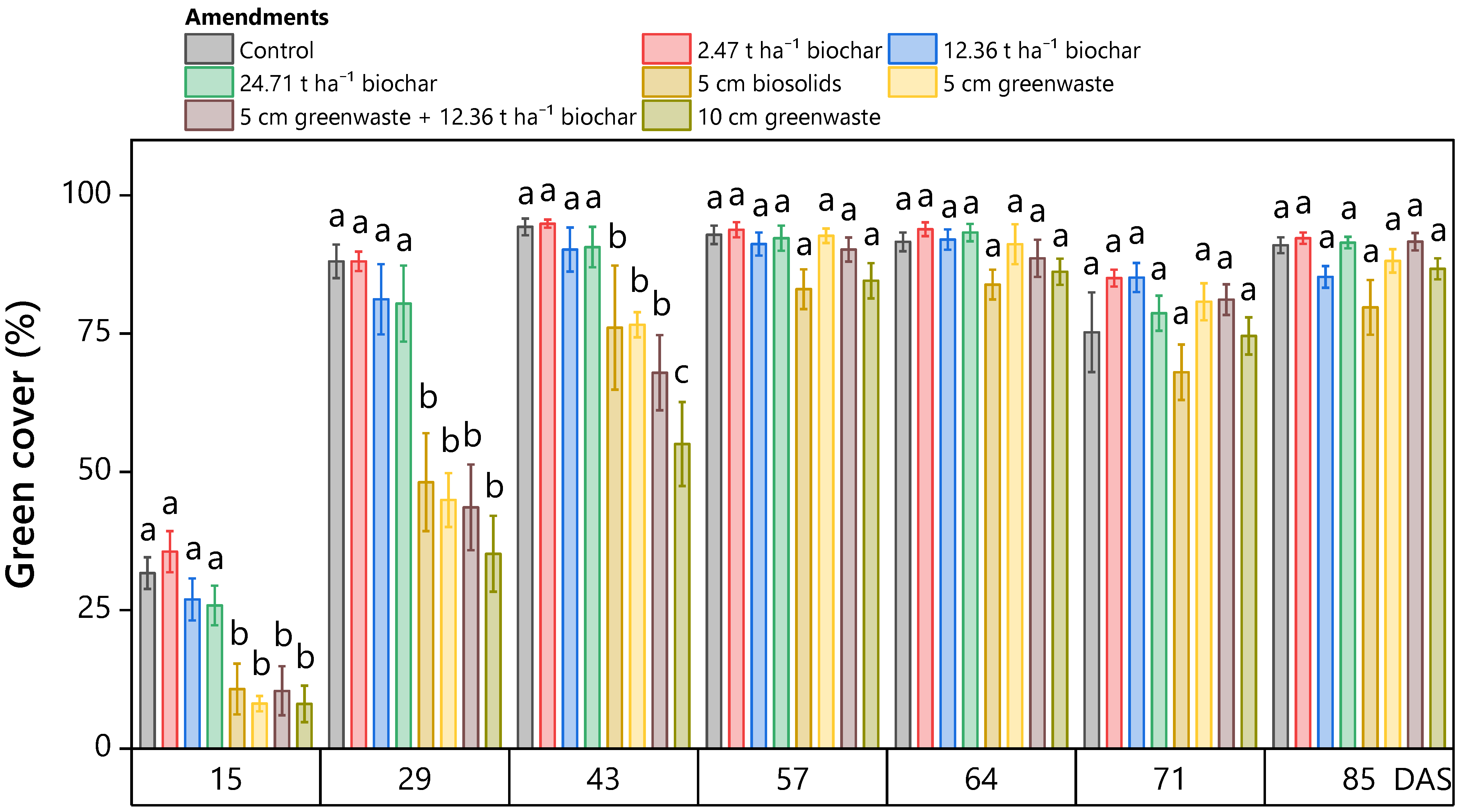
Percentage green cover (PGC) increased across all treatments during the 85-day establishment period, though canopy development trajectories differed significantly among soil amendments (p < 0.05). The heavy organic amendments reduced early stand development relative to the control and biochar treatments.
During the early establishment phase (15–43 days after seeding, DAS), the untreated control and the three biochar rates (T2, T3, T4) exhibited the most rapid emergence. By 15 DAS, these treatments reached approximately 32%, 36%, 27%, and 26% cover, respectively (Figure 2). In contrast, the biosolids (T5) and greenwaste-based treatments (T6, T7, T8) showed significantly lower early PGC values, with the 10 cm greenwaste treatment (T8) reaching only 8% cover at the first evaluation. By 43 DAS, the organic amendments began to accelerate, particularly T7 and T8, although both remained in lower statistical groups (“B” and “C”) relative to the control at this stage (Figure 2).
Between 57 and 85 DAS, sward density converged across treatments. By 57 DAS, the early growth lag in the organic amendments had largely diminished, with most treatments assigned to the “A” or “B” Scott–Knott clusters. By 85 DAS, all treatments achieved statistical uniformity, with PGC values ranging from 80% to 92%, indicating that amendment-driven differences in early growth did not prevent the formation of a contiguous sward prior to the 2015 treatment phase (Figure 2).

Modeling Canopy Trajectories

The development of PGC over time varied with treatment, as reflected in the fitted regression models ( R ¯ 2 = 0.74–0.96; Table S1). For seven of the eight treatments, a square-root model best described the rapid early expansion and subsequent stabilization. The untreated control reached a maximum PGC of 95.50% at 54.3 DAS. Among the biochar treatments, only the 2.47 t ha−1 rate (T2) exceeded the control, reaching 97.46% at 55.9 DAS. The higher biochar rates (T3 and T4) exhibited similar temporal patterns to the control, with peaks between 56 and 58 DAS and maximum PGC values of 94.4–94.6% (Table S1).
The organic amendments displayed more prolonged establishment trajectories. Biosolids (T5) reached a maximum of 80.74% at 64.7 DAS, while the 5 cm greenwaste treatment (T6) peaked at 89.17% at 71.7 DAS. The greenwaste + biochar blend (T7) exhibited the longest establishment period, reaching 90.94% at 87.33 DAS. The 10 cm greenwaste treatment (T8) reached 85.81% at 79.6 DAS and was the only treatment requiring a second-order polynomial model ( R ¯ 2 = 0.94), reflecting its pronounced early lag followed by accelerated late-season canopy closure.

3.2. Canopy Reflectance and Physiological Assessment (2015)

3.2.1. Visual Quality

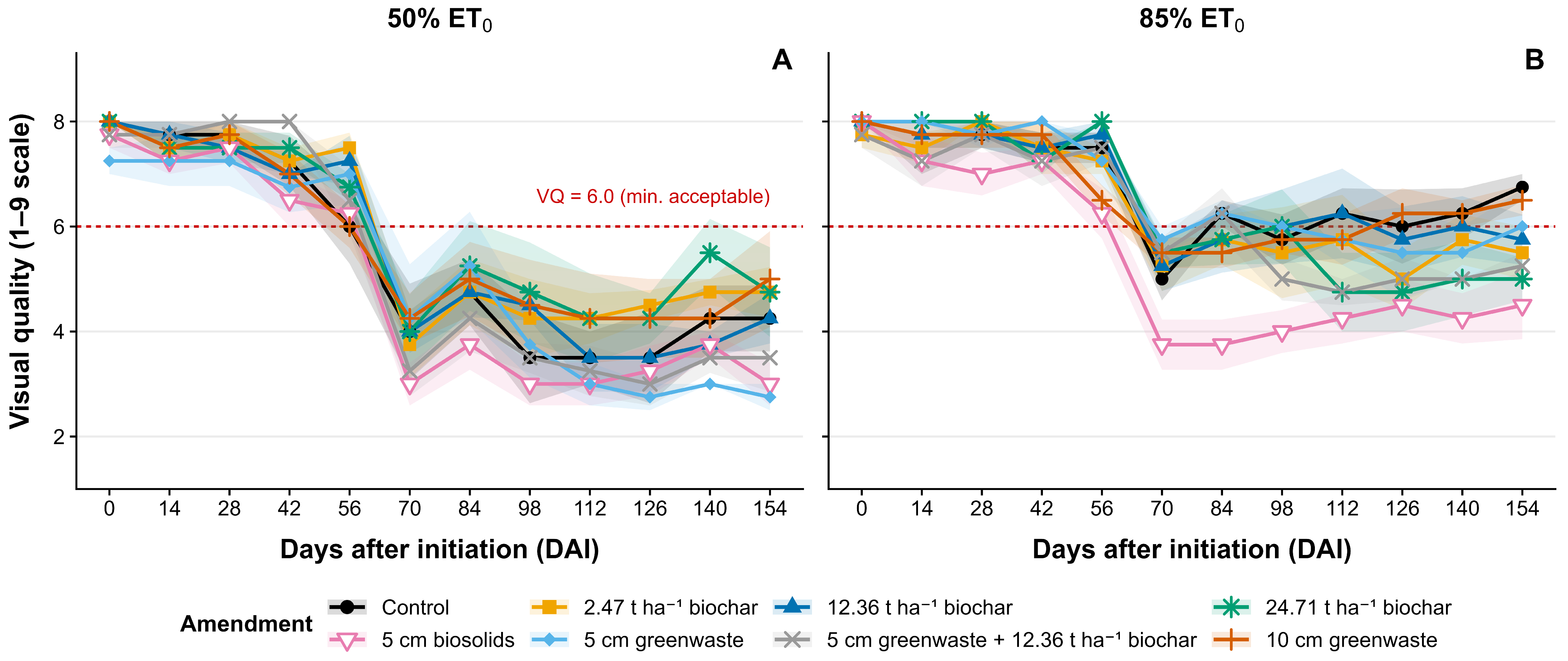
During the early portion of the treatment phase (DAI 0–42), all treatments maintained VQ above the minimum acceptable threshold (VQ ≥ 6.0) under both irrigation regimes, with no significant differences detected among amendments or between irrigation regimes at any of those dates (Table S2).
As the season progressed, VQ declined at rates that varied across irrigation regimes and amendments (Table S3). Under 50% ET0, all treatments followed quadratic or linear trajectories ( R ¯ 2 ≥ 0.70), with no amendment maintaining acceptable quality through the full evaluation period. Modeled minimum VQ values ranged from 3.09 (5 cm biosolids; 141 DAI) to 4.64 (24.71 t ha−1 biochar; 130 DAI). The 12.36 t ha−1 biochar followed a linear trajectory with a projected VQ of 2.98 at 154 DAI.
Under 85% ET0, only the untreated control and 12.36 t ha−1 biochar were best described by constant models above the acceptable threshold (VQ = 6.69 and 6.63, respectively; Table S3), indicating no significant seasonal decline. The remaining treatments followed linear or quadratic decline trajectories, with projected VQ at 154 DAI ranging from 4.39 (24.71 t ha−1 biochar) to 5.20 (5 cm greenwaste). The 5 cm biosolids treatment exhibited the steepest quadratic decline under 85% ET0 ( R ¯ 2 = 0.79), reaching a predicted minimum of 4.06 at 123 DAI. The 10 cm greenwaste treatment followed a similar quadratic pattern ( R ¯ 2 = 0.74), reaching a predicted minimum of 5.81 at 106 DAI before partially recovering later in the season.
Two natural precipitation events punctuated the treatment phase: 29.6 mm fell on 18–20 July 2015 (DAI 75–77), between the DAI 70 and DAI 84 evaluations, and 26.4 mm fell on 9 and 15 September (DAI 128 and 134), between the DAI 126 and DAI 140 evaluations (Figure 1B). Following the July event, VQ improved across all treatments under 50% ET0, with gains ranging from 0.75 to 1.25 points (Table S2). Following the September event, modest gains were observed under 50% ET0, with the 24.71 t ha−1 biochar treatment recording the largest recovery of 1.25 points.
Irrigation Effects and Soil Amendment Effects
Differences between irrigation regimes first became statistically detectable at 56 DAI, when the untreated control recorded significantly lower VQ under 50% ET0 (6.0) than under 85% ET0 (7.5). No significant irrigation effects were observed for the biochar treatments to date. By 98 DAI, significant irrigation effects were present for the untreated control, 5 cm greenwaste, and the 5 cm greenwaste + 12.36 t ha−1 biochar combination, each showing lower VQ under 50% ET0. Thereafter, irrigation effects became more widespread and persistent. The 5 cm greenwaste + 12.36 t ha−1 biochar combination showed significantly lower VQ under 50% ET0 continuously from DAI 70 through DAI 154. The untreated control was significant again from DAI 84 through DAI 154 (the DAI 70 evaluation was a non-significant exception) and 5 cm greenwaste from DAI 98 through DAI 154. The 12.36 t ha−1 biochar treatment showed significant irrigation differences from DAI 112 through DAI 140 and 10 cm greenwaste only at DAI 140 (Table S2).
Under 85% ET0, amendment differences emerged at 70 DAI, when 5 cm biosolids (VQ = 3.75) was assigned to a lower Scott–Knott group than all remaining treatments. By 154 DAI, only the untreated control (VQ = 6.75), 10 cm greenwaste (VQ = 6.50), and 5 cm greenwaste (VQ = 6.00) maintained VQ at or above the minimum acceptable threshold (Table S2).
Under 50% ET0, amendment separation first emerged at 126 DAI, when 2.47 t ha−1 biochar, 24.71 t ha−1 biochar, and 10 cm greenwaste maintained significantly higher VQ than the remaining treatments (Table S2). At 140 DAI, 2.47 t ha−1 biochar and 24.71 t ha−1 biochar (VQ = 4.75 and 5.50, respectively) remained in the higher Scott–Knott group, while 10 cm greenwaste (VQ = 4.25) joined the lower group.
No treatment under 50% ET0 recovered to the acceptable threshold for the remainder of the evaluation period (range 2.75–5.50; Figure 3).
Season-long integrated visual quality, expressed as area under the progress curve (AUPC), differed significantly among soil amendments (F = 2.63; df = 7, 42; p = 0.024), with no amendment × irrigation interaction (F = 0.82; df = 7, 42; p = 0.577; Table 1). Because the interaction was not significant, amendments were compared as a main effect, pooled across irrigation regimes: 5 cm biosolids produced the lowest AUPC and formed a separate group, while the remaining seven amendments did not differ from one another (Scott–Knott; Table 1). AUPC was also significantly higher under 85% ET0 than under 50% ET0 (F = 37.66; df = 1, 3; p = 0.009), with regime means of 973 and 823, respectively.

3.2.2. Normalized Difference Vegetation Index (NDVI)

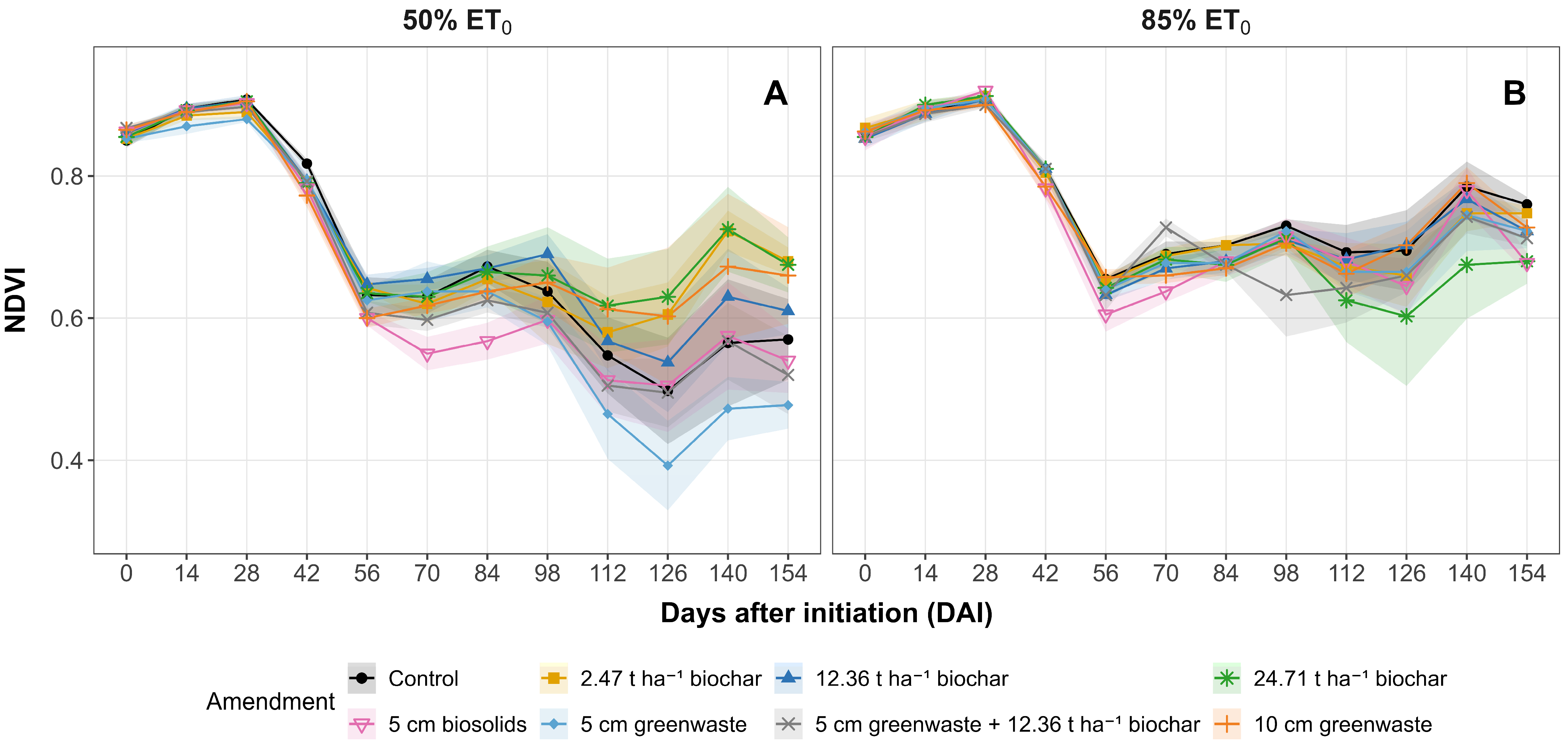
The Normalized Difference Vegetation Index (NDVI) provided an objective measure of canopy greenness and vigor throughout the 154-day treatment period. NDVI values were initially high and uniform across all treatments (0.85–0.92), indicating comparable baseline canopy reflectance at the onset of the irrigation phase. As drought stress intensified under the 50% ET0 regime, NDVI values began to diverge among treatments (Table S4, Figure 4).
Under deficit irrigation, NDVI declined following amendment-specific trajectories (Table S5). The untreated control and the 5 cm greenwaste treatment exhibited steady first-order linear declines ( R ¯ 2 = 0.78 and 0.87, respectively), whereas most other treatments followed second-order polynomial patterns, reflecting non-linear physiological responses to progressive moisture depletion. The 10 cm greenwaste treatment maintained the highest modeled NDVI floor among the second-order trajectories (0.66 at 96.67 DAI), comparable to the 2.47 and 12.36 t ha−1 biochar treatments (0.65 and 0.66; Table S5). The 24.71 t ha−1 biochar treatment reached its minimum later than any other amendment (0.58 at 132.50 DAI), indicating a slower, more delayed decline.
Significant irrigation effects first appeared at DAI 28, when 5 cm greenwaste recorded significantly lower NDVI under 50% ET0 than under 85% ET0 (0.88 vs. 0.91). Irrigation effects became progressively more widespread thereafter, with multiple treatments showing significant differences by 98 DAI. Under the moderate 85% ET0 regime, NDVI values remained comparatively stable, generally staying above 0.60 throughout the evaluation period. In contrast, the deficit regime produced substantial reductions; at 126 DAI, the untreated control declined from 0.70 under 85% ET0 to 0.50 under 50% ET0, representing a 28% reduction in canopy reflectance index (Table S4).
Under the 50% ET0 regime, treatment differences became increasingly pronounced during the peak-stress period (112–154 DAI). Across these dates, the biochar rates and 10 cm greenwaste consistently held the highest Scott–Knott group, while the lower-rate organic amendments (5 cm biosolids, 5 cm greenwaste, and 5 cm greenwaste + 12.36 t ha−1 biochar) grouped lower, and the untreated control declined into the lower group by 154 DAI (Figure 4; Table S4). The gains between DAI 126 and DAI 140 coincided with the September precipitation event (26.4 mm on DAI 128 and 134) and likely reflect a moisture-driven canopy recovery rather than a treatment-specific advantage, since all eight treatments improved over this interval regardless of amendment type (Table S4). At the final evaluation (154 DAI), the highest NDVI values under deficit irrigation were observed with 2.47 t ha−1 biochar (0.68), 24.71 t ha−1 biochar (0.68), and 10 cm greenwaste (0.66), all remaining in the highest group. In contrast, the untreated control and lower-rate organic amendments (5 cm biosolids, 5 cm greenwaste, and 5 cm greenwaste + 12.36 t ha−1 biochar) declined into the 0.48–0.57 range, while 12.36 t ha−1 biochar (0.61) remained in the highest group but was numerically lower than the two higher biochar rates (Table S4).

3.2.3. Dark Green Color Index (DGCI)

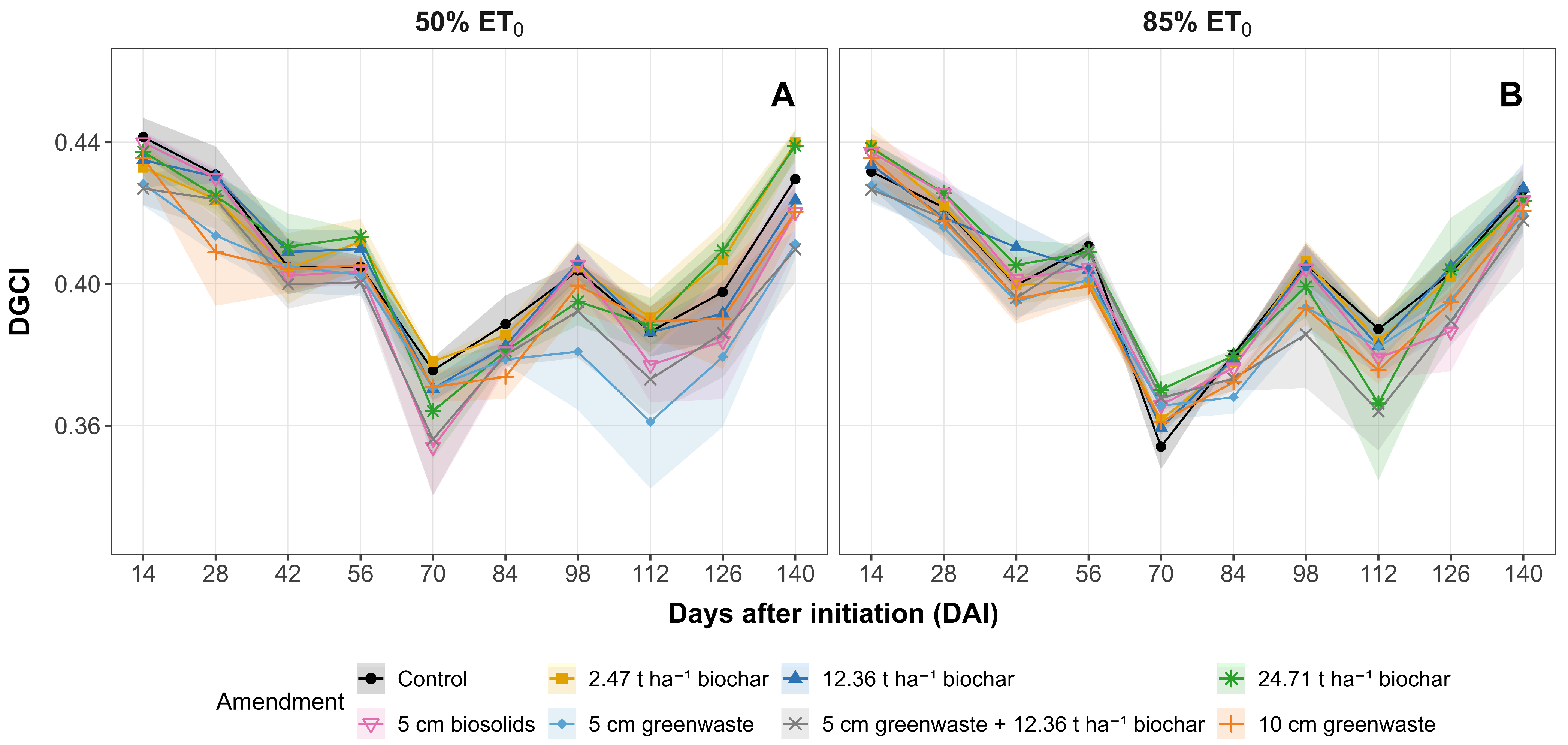
DGCI values remained relatively consistent throughout the evaluation period, ranging from 0.35 to 0.44 across all soil amendments, irrigation regimes, and sampling dates (Table S6, Figure 5). Despite this narrow numerical range, several statistically significant but treatment- and date-specific differences were detected.
Across irrigation regimes, significant differences between the 50% and 85% ET0 levels (lowercase letters) were limited and sometimes ran counter to typical drought expectations. At 70 DAI, the untreated control (T1) and the 2.47 and 12.36 t ha−1 biochar treatments (T2 and T3) exhibited significantly higher DGCI under the 50% ET0 deficit than under 85% ET0, whereas all other treatments showed no irrigation effect at this date. At 140 DAI, T2 again showed a higher DGCI under 50% ET0 (0.44) than under 85% ET0 (0.42). For all remaining treatment-date combinations, no significant differences were detected between irrigation regimes, indicating that canopy color was generally resilient to the imposed deficit (Table S6).
Differences among soil amendments were more evident under the 50% ET0 regime during the latter half of the study, where the untreated control, 2.47 t ha−1 biochar, and 24.71 t ha−1 biochar maintained higher DGCI (0.40–0.44 by 126–140 DAI) than the 12.36 t ha−1 biochar and the organic-based amendments (0.38–0.42). Under 85% ET0, amendment-level differences were largely absent (Table S6, Figure 5).
The most consistent canopy response to precipitation observed across the entire evaluation period was the DGCI recovery following the September event. All eight treatments under 50% ET0 recorded higher DGCI at DAI 140 than at DAI 126, with increases of 0.02 to 0.04 units, representing the only evaluation window in which the full treatment set responded uniformly in the same direction.
Temporal Dynamics of DGCI
The DGCI regression analysis indicated that, although absolute values remained within a narrow range, canopy color exhibited significant temporal structure for a subset of treatment–irrigation combinations.
Under the 85% ET0 regime, most soil amendments were best described by constant models, with fitted mean DGCI values ranging from 0.3949 to 0.4024. In contrast, the 5 cm and 10 cm greenwaste treatments (T6 and T8) followed quadratic models with adjusted coefficients of determination ( R ¯ 2 ) of 0.741 and 0.772, respectively. These models predicted minimum DGCI values of approximately 0.377 at about 83 DAI for T6 and 0.375 at about 84 DAI for T8, after which DGCI values increased slightly toward the end of the monitoring period.
Under the 50% ET0 deficit, only three treatments met the R2adj ≥ 0.70 criterion for quadratic models: the untreated control (T1), 24.71 t ha−1 biochar (T4), and 5 cm greenwaste (T6), with adjusted coefficients of determination of 0.761, 0.711, and 0.709, respectively. For these treatments, DGCI declined to mid-season minima before partially recovering. The fitted curves indicated minimum DGCI values of approximately 0.387 at around 85 DAI for T1, 0.384 at around 81 DAI for T4, and 0.375 at around 92 DAI for T6. The 2.47 t ha−1 biochar treatment (T2) did not reach the R ¯ 2 adj threshold (0.696) and was therefore represented by a constant model rather than a quadratic one. Similarly, the 12.36 t ha−1 biochar, 5 cm biosolids, 5 cm greenwaste + biochar, and 10 cm greenwaste treatments (T3, T5, T7, and T8) under 50% ET0 were also best described by constant models, indicating no statistically significant temporal trend in DGCI for these combinations.
Treatments with High Color Constancy
All remaining treatments under both irrigation regimes, specifically 2.47 t ha−1 biochar, 12.36 t ha−1 biochar, 5 cm biosolids, and 5 cm greenwaste + 12.36 t ha−1 biochar, were best described by constant models.

3.2.4. Pearson’s Correlation

Pearson correlations among canopy performance indicators and soil moisture are presented for both the full evaluation period and the stress period in Table 2. NDVI was most strongly correlated with visual quality in both periods (r = 0.775 and r = 0.733, respectively; p < 0.001). The dark green color index correlated more weakly with visual quality during the stress period (r = 0.141, p < 0.01) than across the full season (r = 0.460). Volumetric water content was moderately and positively correlated with both visual quality (r = 0.591) and NDVI (r = 0.495) during the stress period, whereas its correlation with NDVI was non-significant across the full evaluation period (r = −0.073, p = 0.064). These shifts indicate that the indices captured partly distinct aspects of canopy status, particularly under stress, so canopy condition was interpreted from the three measures together rather than from any single index.

3.3. Soil Hydrological Dynamics (θv)

Volumetric water content (θv) did not exhibit a consistent linear or quadratic temporal pattern. Instead, θv values fluctuated in response to periodic irrigation events, producing high variability across evaluation dates. As specified by the hierarchical regression selection criteria described in the statistical methods, all fitted temporal models produced adjusted coefficients of determination below the 0.70 threshold. Consequently, θv was best represented by treatment-specific means rather than regression equations, reflecting the absence of a meaningful seasonal trend attributable to soil amendments or irrigation regime (Table S7, Figure 6).
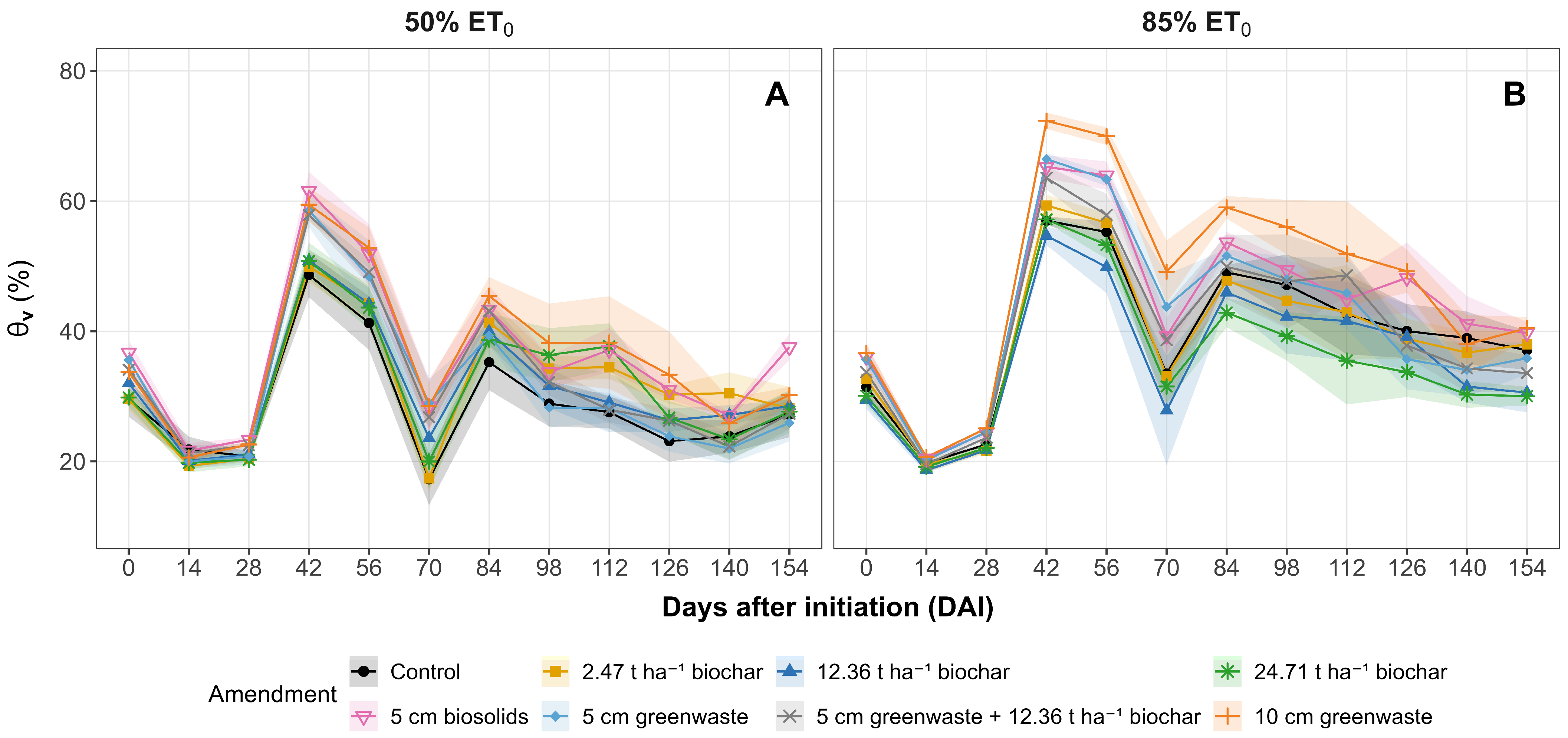
Despite the lack of a temporal trajectory, significant differences in soil moisture magnitude were observed among treatments (p < 0.05). Under the 50% ET0 deficit regime, the untreated control reached its lowest θv of any treatment, whereas several organic amendments held substantially more soil water. Early in the season (42 DAI), the 5 cm biosolids, 5 cm greenwaste, and 10 cm greenwaste treatments exceeded the control by approximately 10–13 percentage points, and at mid-season depletion (112 DAI), the 10 cm greenwaste, 24.71 t ha−1 biochar, and 5 cm biosolids treatments remained significantly wetter than the control, indicating that multiple amendments moderated moisture loss relative to the unamended soil (Figure 6; Table S7).
Under the moderate 85% ET0 irrigation regime, soil moisture remained consistently higher across all treatments. The 10 cm greenwaste treatment (T8) frequently exhibited the highest θv values, reaching 72.33% at 42 DAI compared to 56.98% in the control, an increase of approximately 27%. Even during subsequent depletion cycles, such as at 70 DAI, T8 maintained θv at 49.13%, substantially higher than the control (33.48%). Across the full evaluation period, organic amendments, particularly T5, T6, and T8, consistently elevated θv relative to the untreated control under both irrigation regimes.

3.4. Canopy Growth (2015)

Irrigation regime significantly affected aboveground biomass (p = 0.0268), whereas neither the overall amendment effect (p = 0.1799) nor the amendment × time interaction was significant. Temporal regression analyses indicated no significant linear or quadratic trends for any treatment under either irrigation regime; all 16 treatment–irrigation combinations were best represented by treatment-specific means (Y = ȳ), reflecting the high temporal variability in biomass driven by irrigation events and mowing cycles rather than a progressive seasonal trend.
At 45 DAI, biomass under the 50% ET0 regime exceeded that under 85% ET0 for the untreated control (66.80 vs. 38.01 g m−2), consistent with the significant irrigation main effect. At 101 DAI, biomass under 50% ET0 ranged from 64.9 to 128.7 g m−2, representing increases of 1.3-fold to 2.7-fold relative to 45 DAI, coinciding with the precipitation event recorded on 18–19 July 2015 (Figure 1B). By 129 DAI, biomass declined to a cross-treatment mean of 7.5 g m−2, with no irrigation- or amendment-level differences detected.

3.5. Root Morphology and Architecture (2015)

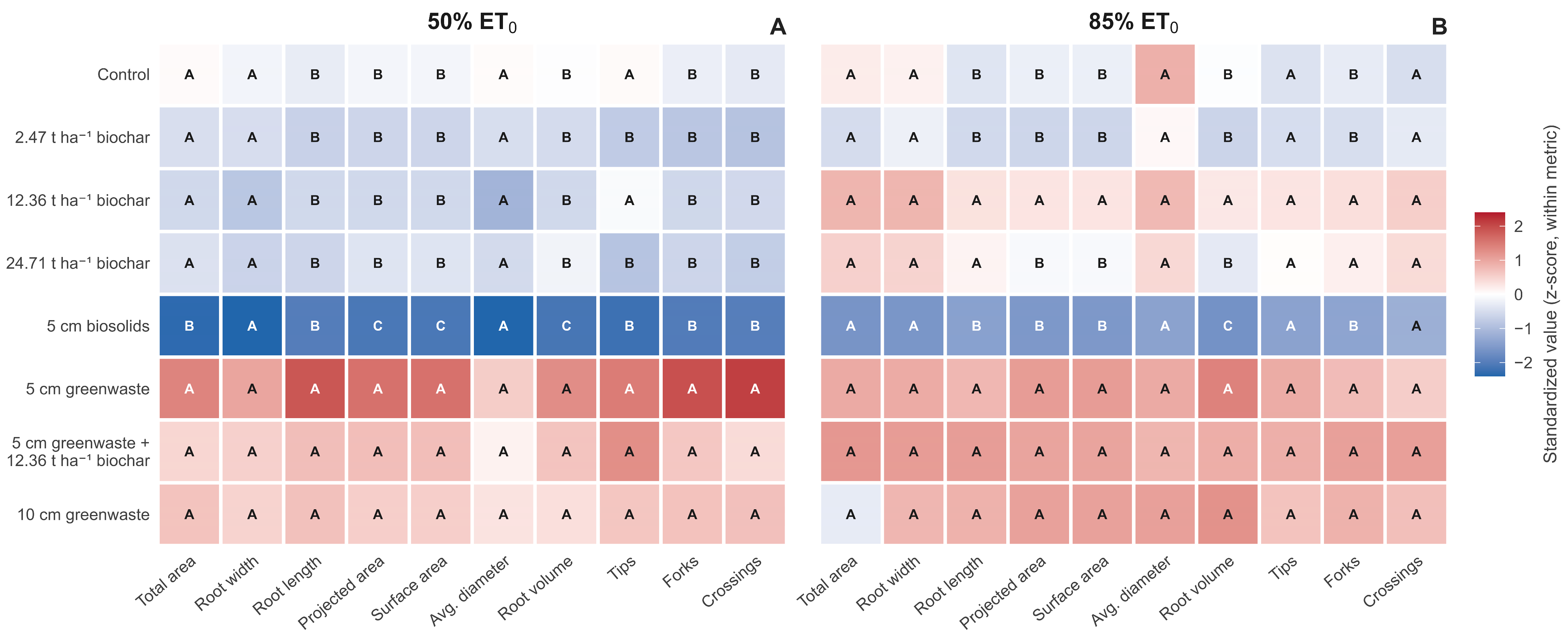
Root development within the upper 12 cm of the soil profile varied significantly among soil amendments, with clear differences in root scale and branching characteristics across treatments (Table S8, Figure 7). Irrigation regime effects were treatment-specific. For the 5 cm biosolids amendment (T5), several root metrics, including total area, root width, total root length, projected area, surface area, and the number of tips, forks, and crossings, were significantly higher under the 85% ET0 regime than under 50% ET0, as indicated by the differing lowercase letters. In contrast, no significant irrigation-level differences were detected for any root metric in the biochar or greenwaste treatments, nor in the untreated control.
Under the 50% ET0 regime, the greenwaste treatment (T6, T7, and T8) formed the highest statistical group for root length, with 5 cm greenwaste numerically greatest (8205.08 cm), significantly exceeding the untreated control, all biochar treatments, and biosolids. Similar patterns were observed for root volume, where the greenwaste treatments (T6, T7, and T8) formed the highest statistical group, while T5 consistently produced the lowest volume (3.47 cm3). T5 also had the lowest projected area (91.86 cm2) and surface area (288.57 cm2) under 50% ET0, placing it in the lowest statistical group for these metrics.
Under 85% ET0, the greenwaste treatments remained in the highest statistical group for both total root length and surface area. For root length, they were joined by the 12.36 and 24.71 t ha−1 biochar treatments; for surface area, by the 12.36 t ha−1 biochar treatment. For example, 10 cm greenwaste produced a total root length of 6575.65 cm, significantly greater than both the biosolids treatment (2881.37 cm) and the untreated control (4556.54 cm).
Branching characteristics followed similar amendment-driven patterns. Under 50% ET0, the greenwaste treatments (T6, T7, and T8) formed the highest statistical group for both forks and crossings, with 5 cm greenwaste numerically greatest (104,680.25 forks and 22,048.50 crossings), significantly exceeding the untreated control, all biochar treatments, and the biosolids amendment. Under the 85% ET0 regime, however, no significant differences among amendments were detected for root crossings, with all treatments grouped together.
Overall, soil amendments exerted strong effects on root size and branching under deficit irrigation (50% ET0), with more limited differentiation under 85% ET0, where several size and branching metrics (total area, root width, diameter, tip number, and crossings) showed no significant amendment separation.

3.6. Soil Nitrogen Dynamics (2015)

Soil nitrate (NO3–N), ammonium (NH4+–N), and total nitrogen (Total N) concentrations were evaluated at two depths (0–15 cm and 15–30 cm) under both irrigation regimes to assess amendment-driven differences in nutrient availability and vertical stratification (Table 3).
At the 0–15 cm depth, significant irrigation effects on NO3–N were detected only for the untreated control and the 24.71 t ha−1 biochar treatment, both of which exhibited higher NO3–N under 50% ET0 than under 85% ET0. For all other amendments at this depth, NO3–N did not differ significantly between irrigation regimes. For Total N, irrigation-level differences at 0–15 cm were also limited to specific treatments, including the untreated control, 24.71 t ha−1 biochar, and the 5 cm greenwaste + 12.36 t ha−1 biochar combination, all of which showed higher Total N under 50% ET0.
At the deeper 15–30 cm depth under 85% ET0, NO3–N concentrations did not differ among any of the eight amendments, with all treatments assigned to the same statistical group, indicating that amendment effects on NO3–N were not detectable at this depth under the higher irrigation volume.
Soil amendments differed markedly in nitrogen availability. The 5 cm biosolids treatment consistently produced the highest NO3–N and Total N concentrations at both depths under both irrigation regimes. At 0–15 cm depth under 50% ET0, biosolids exhibited the highest NO3–N (6.33 mg kg−1) and Total N (8.14 mg kg−1), significantly exceeding those of the untreated control and all biochar and greenwaste treatments. In contrast, the greenwaste treatments and 12.36 t ha−1 biochar formed the lowest statistical group for Total N at this depth, with values ranging from 3.13 to 3.77 mg kg−1.
Vertical stratification of nitrogen was evident in several treatments, although Table 3 does not provide direct statistical comparisons between depths. Under 50% ET0, Total N in the 24.71 t ha−1 biochar treatment was higher at 0–15 cm (5.78 mg kg−1) than at 15–30 cm (3.37 mg kg−1). Under 85% ET0, NO3–N in the 5 cm greenwaste treatment was numerically greater at 0–15 cm (1.26 mg kg−1) than at 15–30 cm (0.80 mg kg−1), and NH4+–N in the 12.36 t ha−1 biochar treatment was higher at 0–15 cm (1.22 mg kg−1) than at 15–30 cm (0.49 mg kg−1). These differences reflect the distribution patterns shown in Table 3, although the associated p-values for depth comparisons originate from separate analyses not included in the table.
The biosolids consistently produced the highest nitrogen concentrations across depths and irrigation regimes, while greenwaste-based amendments exhibited the lowest NO3–N values under deficit irrigation at both depths, and the greenwaste and 12.36 t ha−1 biochar treatments together formed the lowest Total N group at the 0–15 cm depth under 50% ET0.

4. Discussion

4.1. Canopy Responses Relative to Soil Water Availability

The most counterintuitive finding from this study was not which treatment performed best, but which one did not. The 10 cm greenwaste layer consistently held the highest volumetric water content across the experimental period, an outcome consistent with its high porosity and capacity to buffer evaporative losses. Yet it is equally plausible that the poorer canopy under greenwaste plots simply reduced transpirational demand, leaving more water in the profile, a stress-driven outcome rather than an amendment benefit. Under this interpretation, high soil moisture would be a consequence of canopy decline rather than a cause of canopy maintenance.
Even with its clear moisture advantage, the 10 cm greenwaste treatment could not convert water availability into photosynthetic vigor. At 126 DAI under the 50% ET0 regime, the 24.71 t ha−1 biochar treatment maintained a numerically higher NDVI (0.63) despite holding less total water in the profile. The 10 cm greenwaste treatment, by contrast, recorded an NDVI of 0.60; that is, a treatment with lower soil moisture sustained a healthier canopy than one with substantially more moisture, which points to the nutritional and architectural quality of the root-zone environment as being more closely tied to canopy maintenance than raw water-holding capacity.
No treatment, however, sustained acceptable visual quality (VQ ≥ 6.0) under 50% ET0 beyond DAI 56. By DAI 70, all treatments had declined below the threshold regardless of amendment type. The biochar advantage documented above is therefore relative: biochar treatments maintained higher NDVI during the stress period but did not prevent quality decline under severe deficit. Biochar moderated the decline; it did not prevent it.
The mechanistic basis for why biochar modulates soil water is reasonably well established. Its internal pore architecture shifts water retention toward finer capillary fractions, increasing plant-available water at the expense of drainable macropores, a shift that Blanco-Canqui [38] documented across a wide body of literature, finding that biochar increased plant-available water in 72% of evaluated cases. Abel et al. [39] showed that biochar reshapes the water retention curve through bimodal pore distributions rather than simple bulk effects, and Zhang et al. [40] identified nitrogen- and oxygen-containing surface moieties as hydrogen-bond receptors that suppress evaporation from bound-water domains. Together, these lines of evidence describe a coherent mechanism: biochar retains water in forms that roots can access and slows the loss of what it holds. Recent field evaluations on coarse-textured, drought-prone soils confirm this behavior, with combined biochar and organic amendments sustaining elevated soil water content through prolonged dry-down periods [41], and improved soil hydraulic conditions have been linked to deeper rooting and maintained photosynthetic function under drought [42].
NDVI alone, however, does not fully capture canopy response to biochar. Horel and Tóth [43] monitored biochar-amended and unamended sweet corn plots across two growing seasons, measuring NDVI alongside the photochemical reflectance index (PRI) and fraction of absorbed photosynthetically active radiation (fAPAR). Their results were instructive precisely because the indices disagreed: control plots showed marginally higher NDVI, while biochar-amended plots exhibited substantially higher PRI (+26.8%) and fAPAR (+2.24%), suggesting that actual photosynthetic efficiency was superior in the biochar treatment despite a slightly lower reflectance index. Notably, both NDVI and fAPAR were negatively correlated with soil water content (−0.59 < r < −0.30; p < 0.05), so in their study, high soil moisture did not translate into superior canopy performance. The present data show the same decoupling over the full season, where θv was at best a weak predictor of canopy performance; the relationship strengthened only during the peak-stress window (θv–VQ = 0.59, θv–NDVI = 0.50), when plots retaining more water tended to sustain marginally better canopies.
The precipitation-recovery episodes documented across multiple variables offer the most direct evidence that the canopy remained biologically active throughout the evaluation period. Following the July event, θv increased in all eight treatments under 50% ET0 between DAI 70 and DAI 84. VQ improved across all eight treatments, DGCI increased in seven of eight, and the DAI 77 clipping demonstrated that active shoot growth was already underway. The DAI 101 biomass surge (64.9 to 128.7 g m−2 under 50% ET0) reflects the full metabolic response to that single replenishment event. The September precipitation produced a parallel signal: DGCI recovered in all eight treatments, and VQ improved in seven, with 10 cm greenwaste the sole exception, holding at 4.25 at both DAI 126 and 140.
Gravimetric biomass, soil moisture, visual quality rating, active optical sensing, and digital image analysis, five methods, each operating on a different physical principle, all tell the same story: this was a stand under stress, but never one that had stopped growing. Among the canopy indicators, specifically, visual quality, NDVI, and DGCI are complementary rather than equivalent. They respond to different things: NDVI to canopy density and greenness, DGCI to chlorophyll and color (and therefore sensitive to illumination), and visual quality to integrated appearance. Spectral reflectance and digital image analysis are established but not interchangeable correlates of turfgrass quality [44]. Because of these differing sensitivities, treating the indices as a single aggregated measure of physiological status would risk mischaracterizing canopy condition, and that risk is greatest under stress, when their agreement weakens (Section 3.2.4). Where the three agreed in direction here, we read their convergence as corroboration across independent methods rather than as one aggregated index of physiological status.

4.2. Root System Responses to Soil Amendments

Greenwaste at both application depths produced the most extensive root systems, with total root length, surface area, volume, and branching complexity all markedly higher than in the other treatments. These are precisely the metrics that respond most predictably to improved soil physical conditions: reduced bulk density, better aeration, and lower penetration resistance, conditions that Bengough et al. [45] identified as rate-limiting for root elongation, where resistances above roughly 0.8–2 MPa or matric potentials drier than −0.5 MPa were each sufficient to halve elongation rate. Greenwaste attenuates both stresses simultaneously.
Biosolids treatment produced the opposite outcome, with the lowest values across every root morphological metric. Two stresses converged. Osmotically, the high ionic load in freshly applied biosolids would reduce water availability at the root surface before any tissue-level toxicity manifests, the rapid osmotic phase of salinity stress described by Munns and Tester [46]. Chemically, Section 3.6 shows that the biosolids treatment produced Total N concentrations 1.2–2.1 times higher than the untreated control across depths and irrigation regimes, a loading consistent with the range where nitrogen availability exceeds plant uptake capacity and enters phytotoxic territory; turfgrass guidelines generally place the threshold near 48.8 kg ha−1 per application. The root system was not simply failing to grow; it was operating in a root zone where both water stress and chemical excess limited meristematic activity.
That several root metrics were significantly higher for biosolids under 85% ET0 than under 50% ET0 is most simply explained by drought physiology. Cool-season grasses require approximately 75–80% ET0 replacement to avoid water stress, and the 50% ET0 regime fell well below that threshold. Water deficit alone was sufficient to suppress root growth independently of the amendment’s chemical load, and since both irrigation levels remained below field capacity, no net downward nutrient movement occurred. The partial recovery under 85% ET0 reflects relief from water stress, not dilution of phytotoxic compounds. Huang and Fry [47] confirmed that root length, surface area, and branching are among the most stress-responsive morphological indicators in tall fescue, which supports the interpretation that what the data show here is a genuine biological signal.

4.3. Nitrogen Dynamics Across Organic and Biochar Amendments

The nitrogen data from this study reveal something that the canopy and root results alone could not: each amendment class operated under a fundamentally different nitrogen logic, and understanding these distinct pathways goes a long way toward explaining the whole-plant response patterns observed above.
The biosolids treatment (T5) consistently produced the highest NO3–N and total N concentrations across sampling depths, and this was especially pronounced in the 15–30 cm layer under deficit irrigation. White et al. [48], synthesizing results from a multi-year biosolids research program across rangeland and agronomic systems, noted that biosolids reliably elevate soil nitrate-nitrogen and that this nitrogen migrates downward through the profile at rates that vary with season and irrigation volume. The nitrogen enrichment in T5, in other words, reflects the fertilizer character of biosolids rather than any failure of the treatment; high plant-available N was present, and some of it moved to depth. Whether that deep nitrogen was accessible to plants depended entirely on root distribution, and in the biosolids treatment, root development was severely suppressed at precisely the depth where nitrogen was most concentrated, as documented in Section 4.2.
The high-rate biochar treatment told a different story. Rather than pushing nitrogen downward, it concentrated more of it in the 0–15 cm layer, the zone where tall fescue roots under post-establishment conditions would be most able to intercept it. This is consistent with what biochar’s physical and chemical properties would predict. Laird et al. [49], in a controlled column leaching experiment using Midwestern agricultural soil amended with swine manure and four rates of biochar, found that the highest biochar rate (20 g kg−1) reduced total nitrogen leaching by 11% and total dissolved phosphorus leaching by 69% even as the biochar itself contributed additional nutrients to the columns, a counterintuitive result that reflects how strongly biochar’s pore structure and surface charge retain applied nutrients. Clough and Condron [50], introducing a Special Issue on biochar and the nitrogen cycle in the Journal of Environmental Quality, synthesized the mechanistic basis for this effect: biochar elevates soil cation exchange capacity and provides adsorptive surfaces for ammonium, suppressing its conversion to the more mobile nitrate form and keeping nitrogen biologically accessible in the surface horizon. Field-scale responses are nonetheless variable, as biochar’s net effect on mineral nitrogen reflects the interacting influences of adsorption, microbial activity, and soil moisture [51]. In the present study, this behavior under deficit irrigation, where reduced water flux would further limit downward nitrogen transport, would compound biochar’s inherent retention advantage.
The greenwaste treatments present the most interpretively demanding pattern. Despite maintaining the highest volumetric water content in the profile, they consistently showed the lowest mineral nitrogen concentrations, particularly at 0–15 cm under 50% ET0. This combination, abundant moisture and nitrogen scarcity, is consistent with microbial nitrogen immobilization. Greenwaste has a high C:N ratio, and when a high-C:N substrate enters the soil, decomposing microorganisms encounter more carbon than their biomass can accommodate without additional nitrogen. They respond by taking up available inorganic N to balance their cellular stoichiometry, temporarily removing it from the plant-available pool. Robertson and Groffman [52], in their comprehensive treatment of soil nitrogen transformations in soil microbiology, ecology, and biochemistry, describe this immobilization dynamic as a standard consequence of organic matter inputs with C:N ratios above approximately 25:1, a threshold that greenwaste compost commonly exceeds. Under deficit irrigation, where reduced soil moisture already suppresses overall microbial activity and mineralization rates, this immobilization effect may have been moderated in absolute terms, as Borken and Matzner [53] review evidence that drying events curtail the microbial processing that would otherwise release or sequester mineral N, but the direction of the effect (toward lower plant-available N in greenwaste plots) remained consistent across both irrigation regimes. The greenwaste treatments were not water-limited in any strict sense, and the data are consistent with nitrogen limitation driven by the high C:N substrate and the biological activity that elevated moisture supported (although reduced plant demand cannot be excluded; see Section 4.6).
This contrast between compost-type and biochar-type amendments in their effects on soil nitrogen has been observed before in a context close enough to the present study to be directly informative. Azeem et al. [54], working with tall fescue establishment plots amended with green waste compost and two rates of biochar, the same amendment classes used here, found that compost-amended soils exhibited nitrogen-induced respiration 94% higher than the unamended control, while soils amended with biochar were statistically indistinguishable from the control in both microbial community composition and N-cycling activity. That divergence is not incidental. Compost introduces large quantities of labile carbon that decomposing microorganisms can metabolize readily, and in doing so, they draw down the inorganic nitrogen pool to meet their stoichiometric needs, the immobilization response that Robertson and Groffman [52] describe as a predictable consequence of high-C:N organic inputs. Biochar does not trigger this response. As DeLuca et al. [55] explain, biochar’s highly aromatic, condensed carbon matrix is largely resistant to microbial attack at agronomic timescales, meaning it can improve soil physical and chemical properties, including ammonium retention and moderated nitrate mobility, without creating the nitrogen sink that compost-type amendments impose during the critical window of plant establishment. The pattern observed in the nitrogen stratification data of the present study is, in that sense, a predictable outcome of a well-documented mechanistic difference between labile and recalcitrant soil carbon sources.

4.4. Implications for Long-Term Soil Amendment Performance

The patterns observed over this two-season experiment point toward something that a single season of data rarely can: the performance trajectories of biochar and compost-type amendments are likely to diverge over time, and not necessarily in the direction that first-season results would suggest. The 10 cm greenwaste layer delivered the largest soil moisture reservoir during the post-establishment phase, a genuine advantage; the organic matter underpinning the benefit is biologically labile. Khaleel et al. [56], synthesizing physical soil responses to organic waste applications across 12 studies, 21 soil types, and 7 waste types, documented strong linear relationships between organic carbon additions and improvements in bulk density and water-holding capacity. The biological availability of that carbon is precisely what makes compost-type amendments transient: as decomposition proceeds, the structural matrix that holds water and reduces compaction is progressively consumed. The amendment that helps most in year one may be the least durable over a decade.
Biochar operates on a fundamentally different timescale. Lehmann et al. [57] demonstrated that pyrolysis converts biomass carbon to a form that retains approximately 50% of its initial carbon, far more than the 3% retained after burning and the negligible fraction surviving biological decomposition, with consequent improvements to soil fertility that cannot be eroded by the microbial community in any agronomically meaningful timeframe. Spokas [58] established that biochars with oxygen-to-carbon molar ratios below 0.2 carry estimated half-lives exceeding 1000 years, while intermediate-quality biochars with higher O:C ratios persist for centuries. The 350 °C pyrolysis temperature used in this study falls in the lower production range; absent direct O:C characterization of this material, a conservative estimate of multi-decadal to centennial persistence is warranted, sufficient to substantially outlast any compost-derived amendment on a management timescale. The physical and chemical modifications that biochar induces in soil pore architecture, cation exchange capacity, and water retention are, in practical terms, durable across the management lifetime of any turf or landscape system. This persistence supports the use of biochar as a durable soil conditioner for sustaining soil function under increasingly drought-prone conditions [59].
Evidence from the same experimental context suggests that differences in amendment longevity become behaviorally meaningful within a few years of application. Hale et al. [11], following up on Azeem et al. [54] in the same tall fescue plots at the University of California, Riverside, found that microbial biomass in compost-amended soils remained 127–157% higher than in unamended controls five years after a single application and that deficit irrigation shifted microbial community structures more strongly in unamended soils than in amended ones. These are soil biology outcomes, not canopy outcomes, but they indicate that both amendment classes continued to buffer the root-zone environment against water stress well beyond the first season. Biochar’s contributions, enhanced pH and water-holding capacity, are expected to persist even longer given its chemical resistance to decomposition, consistent with the persistence literature reviewed by Lehmann et al. [57] and Spokas [58].
Under deficit irrigation, the practical advantage of biochar was not that it prevented quality decline (no amendment did) but that it moderated the depth of that decline. The high-rate biochar treatment held the highest modeled minimum visual quality (VQ) among the top NDVI performers through the stress period, though all treatments fell below the acceptable VQ threshold by DAI 70 under 50% ET0. This advantage was not uniform: 10 cm greenwaste tracked the biochar treatments in the higher NDVI and visual-quality groups at several dates under deficit irrigation, while the lower-rate organic amendments consistently grouped lower. Blum [60] argued that the productive target under water limitation is not narrow water-use efficiency per se but the effective use of water, the deployment of available moisture into productive transpiration. Biochar does not necessarily reduce total soil water demand but reorganizes pore architecture to alter water availability. Whether this advantage compounds over subsequent seasons as greenwaste mineralization progresses and biochar continues to persist remains an open question that the mature-stand evaluation in Part II addresses directly.
That this evidence was gathered during an establishment-year campaign conducted several years ago does not lessen its present relevance, and within a longitudinal program, it arguably increases it. The behaviors documented here are governed by soil processes that unfold over years rather than by the conditions of any single season: the transient hydrological advantage of labile greenwaste and the slower but more durable restructuring attributable to recalcitrant biochar are properties of the amendments themselves, not artifacts of when they were measured. As the first-year baseline of a continuously studied site, this dataset anchors the trajectory whose later stages are captured by the soil-biological responses discussed above and by the mature-stand evaluation in Part II, and its interpretive value grows as that series lengthens. The mandated deficit imposed here, meanwhile, has become an increasingly common condition for municipal turf rather than an experimental extreme, which keeps the establishment-year benchmark it provides directly applicable to present-day management decisions.

4.5. Study Limitations and Future Directions

There are four aspects where the temporal, spatial, and methodological boundaries of the experiment leave important questions open. The first concern is the biosolids treatment. The root suppression documented here was pronounced, with the lowest values across all root morphological metrics, and the most plausible explanation is that osmotic stress from initial salt loading, coupled with an ammonium spike from freshly applied biosolids, created a chemically restrictive environment for root elongation during the critical post-establishment window. Whether that represents a transient chemical environment or a lasting agronomic liability is something a single post-establishment evaluation period cannot resolve. Biosolids are not static inputs: their nutrient chemistry shifts as ammonium nitrifies, electrical conductivity moderates as soluble salts equilibrate with the surrounding soil matrix, and the organic fraction mineralizes. Future work should examine whether lower application rates, pre-leaching of biosolids prior to planting, or delayed seeding can mitigate the initial root suppression observed during this post-establishment evaluation, thereby separating the long-term fertilizer value from early-phase salinity or ammonium stress.
The second limitation involves the carbon-nitrogen dynamics of the greenwaste treatments, which were only partially resolved within the study period. The immobilization inferred in Section 4.3 may be a transient phase rather than a permanent feature: Bernal et al. [61] describe how the labile carbon fraction driving microbial N demand is progressively depleted as compost matures so that nitrogen held in microbial biomass may later be released in plant-available forms. Biochar, by contrast, is recalcitrant on agronomically relevant timescales (Section 4.4) [62]. Whether the two amendment classes eventually converge as greenwaste carbon depletes or whether biochar’s structural permanence continues to produce distinct agronomic outcomes over a multi-year horizon is a question this dataset cannot answer, but long-term monitoring could.
The third limitation is spatial, and it is more accurately characterized as a depth-of-sampling constraint on the nitrogen data than on the root data. Root sampling to 12 cm captured the primary zone of root activity for a first-year turfgrass stand, where the large majority of root mass is concentrated in the upper profile. The more consequential gap is in soil nitrogen characterization, which extends only to 30 cm. Amendment effects on nutrient availability in deeper horizons, particularly any differential retention or mobility between biochar and organic amendments below the root-zone sampling depth, remain unresolved. Future studies incorporating deeper soil cores and more spatially resolved nitrogen profiling would help determine whether the stratification patterns documented here persist or reverse with depth, and whether amendment-driven differences in subsoil nitrogen availability contribute to the canopy and root responses observed at the surface.
A fourth limitation is methodological. Under field conditions, spatial soil heterogeneity and small-scale moisture variability cannot be fully eliminated, and both bear on how the factorial interactions should be read. The randomized complete block design, with four replications and irrigation as the main plot factor, was intended to contain these effects, but the split-split-plot structure tests the irrigation main effect against a whole-plot error term with few degrees of freedom, limiting its power, and within-block variation in the coarse-textured Hanford soil may have narrowed the realized contrast between the 50% and 85% ET0 regimes. Where moisture variability compresses that contrast, true irrigation × amendment interactions are harder to detect, so the non-significant interactions reported here are best read as limited evidence of largely independent responses rather than proof that no interaction exists. Continuous in situ moisture sensing, greater whole-plot replication, or spatial covariate adjustment would help separate genuine interactions from field-scale heterogeneity.

4.6. Integrated Interpretation of Greenwaste Hydrology and Nitrogen Availability

The 10 cm greenwaste treatment yields what is perhaps the most interpretively interesting result of the study: a treatment that performed well on one soil metric and poorly on another, and whose above- and below-ground responses only make sense when considered together. Volumetrically, the greenwaste plots held more water than any other treatment across most of the evaluation period, an outcome consistent with the high organic matter content and improved aggregation that thick surface-applied compost layers confer. Yet under deficit conditions, canopy color and quality in those same plots were generally lower than in the high-rate biochar treatment, and surface-layer total nitrogen was among the lowest recorded. Water abundance and plant performance pointed in opposite directions.
One explanation consistent with this outcome is the nitrogen immobilization described in Section 4.3 [52]. However, an equally plausible explanation is that a canopy already stressed by deficit irrigation and poor performance simply demands less nitrogen, and the low soil N in greenwaste plots reflects reduced plant uptake rather than microbial sequestration. The available data cannot distinguish between these two explanations. What can be said is that the observed combination, high soil moisture, low mineral nitrogen, and reduced canopy performance, is internally consistent, regardless of which mechanism drove it.
Root data adds a further dimension to this picture. The elevated branching intensity and root tip density observed in the greenwaste treatments are consistent with a foraging response in a soil where mineral nitrogen is heterogeneously distributed [63], though the direction of causality is not determinable from morphological data alone. The plant may have been responding to genuine nitrogen scarcity, or the root architecture may simply reflect the physical properties of the greenwaste-amended soil.
The low surface-layer total nitrogen in the 12.36 t ha−1 biochar treatment presents a parallel interpretive challenge. Under adequate irrigation (85% ET0), this treatment maintained among the highest canopy performance values in the study, yet soil N was not markedly different from some of the poorer-performing treatments. Without a calibration curve relating soil nitrogen concentration to tall fescue performance, it is not possible to classify any observed N value as limiting or sufficient from these data alone. What the biochar and greenwaste treatments share is a similarly low soil N reading arrived at under very different performance outcomes, a divergence that points toward soil nitrogen availability being one factor among several, rather than the primary determinant of canopy response in this system.

5. Conclusions

What mattered for tall fescue under deficit irrigation was not any single soil property but how each amendment balanced three things at once: water retention, nitrogen supply, and root development. No amendment managed all three well, and none kept the turf acceptable under the severe deficit. Under sustained 50% ET0, every treatment fell below the visual-quality threshold (VQ ≥ 6.0) by 70 days after initiation and remained there, a reminder that tall fescue has physiological limits that soil management cannot overcome in a climate this dry.
The treatments are still separated in ways worth noting. High-rate biochar (24.71 t ha−1) held the highest modeled minimum visual quality and stayed among the best for NDVI through the stress period; it slowed the decline but did not stop it. Greenwaste held more water than anything else yet carried the least mineral nitrogen near the surface, and that extra water never turned into a better canopy. Whether that was because its high C:N ratio tied up nitrogen, because a struggling canopy simply needed less, or some of both, the data cannot say. Biosolids were the mirror image: the most nitrogen at both depths but the weakest root systems we measured, which is what one would expect if the nitrogen load were high enough to be toxic at this rate. None of these responses can be considered in isolation. Water, nitrogen, and canopy condition fed back on one another under deficit since a thinning canopy transpires less and leaves more water in the soil, so the data cannot tell us how much each one contributed, and soil moisture by itself was a poor guide to turf conditions.
The practical lesson is that choosing an amendment for deficit-irrigated turf means weighing water, nutrients, and the root zone together, not banking on water retention alone. Greenwaste will likely need supplemental nitrogen to be worth its moisture benefit; biosolids deserve caution at this rate until it is clear whether the root suppression is temporary; and high-rate biochar came closest to holding quality, though even it fell short under 50% ET0 in this first year. Whether that biochar advantage lasts as the soil matures is the question Part II takes up.

Supplementary Materials

The following supporting information can be downloaded at: https://www.mdpi.com/article/10.3390/agronomy16131283/s1, Table S1: Regression parameters for the temporal development of the percentage of green cover (PGC) under soil amendments; Table S2: Visual quality (VQ) evaluations of tall fescue as influenced by irrigation regimes and soil amendments; Table S3: Regression parameters for the temporal decline of visual quality (VQ) under 50% and 85% ET0 irrigation regimes; Table S4: Normalized difference vegetation index (NDVI) evaluations of tall fescue canopy vigor as influenced by irrigation regimes and soil amendments; Table S5: Regression parameters for the temporal dynamics of the normalized difference vegetation index (NDVI) under two irrigation regimes; Table S6: Dark green color index (DGCI) evaluations of tall fescue canopy vigor as influenced by irrigation regimes and soil amendments; Table S7: Volumetric water content (θv) evaluations of the soil profile as influenced by irrigation regimes and soil amendments; Table S8: Total area, root width, root length, measured projected area, surface area, average diameter, root volume, number of tips, forks, and crossings of roots in tall fescue across irrigation regimes and soil amendments.

Author Contributions

Conceptualization, J.M. and M.E.M.J.; methodology, J.M. and M.E.M.J.; formal analysis, J.B.S.F.; investigation, J.B.S.F. and J.M.; resources, J.M. and J.B.S.F.; data curation, J.M.; writing—original draft preparation, J.B.S.F. and J.M.; writing—review and editing, J.B.S.F., M.E.M.J., M.S. and J.M.; visualization, J.B.S.F. and M.E.M.J.; supervision, M.E.M.J.; project administration, M.E.M.J.; funding acquisition, M.E.M.J. All authors have read and agreed to the published version of the manuscript.

Funding

This research received no external funding.

Data Availability Statement

The original contributions presented in this study are included in the article/Supplementary Material. Further inquiries can be directed to the corresponding authors.

Acknowledgments

The authors would like to thank the National Council for Scientific and Technological Development (CNPq, Brazil) for the support provided through the Science without Borders Program. We also extend our gratitude to the Department of Botany and Plant Sciences at the University of California, Riverside, for providing the facilities and technical support necessary to conduct this research.

Conflicts of Interest

The authors declare no conflicts of interest.

References

  1. McDonald, R.I.; Weber, K.; Padowski, J.; Flörke, M.; Schneider, C.; Green, P.A.; Gleeson, T.; Eckman, S.; Lehner, B.; Balk, D.; et al. Water on an urban planet: Urbanization and the reach of urban water infrastructure. Glob. Environ. Change 2014, 27, 96–105. [Google Scholar] [CrossRef]
  2. Overpeck, J.T.; Udall, B. Climate change and the aridification of North America. Proc. Natl. Acad. Sci. USA 2020, 117, 11856–11858. [Google Scholar] [CrossRef] [PubMed]
  3. He, C.; Liu, Z.; Wu, J.; Pan, X.; Fang, Z.; Li, J.; Bryan, B.A. Future global urban water scarcity and potential solutions. Nat. Commun. 2021, 12, 4667. [Google Scholar] [CrossRef] [PubMed]
  4. Beard, J.B.; Green, R.L. The role of turfgrasses in environmental protection and their benefits to humans. J. Environ. Qual. 1994, 23, 452–460. [Google Scholar] [CrossRef]
  5. Kjelgren, R.; Montague, T. Urban tree transpiration over turf and asphalt surfaces. Atmos. Environ. 1998, 32, 35–41. [Google Scholar] [CrossRef]
  6. Schiavon, M.; Shiflett, S.; Baird, J.H.; Geis, L.A.; Scudiero, E. Southern California land surface temperature differences under different landscape composition. Agron. J. 2024, 116, 2678–2689. [Google Scholar] [CrossRef]
  7. Hilaire, R.S.; Arnold, M.A.; Wilkerson, D.C.; Devitt, D.A.; Hurd, B.H.; Lesikar, B.J.; Lohr, V.I.; Martin, C.A.; McDonald, G.V.; Morris, R.L.; et al. Efficient water use in residential urban landscapes. HortScience 2008, 43, 2081–2092. [Google Scholar] [CrossRef]
  8. Zere Taskin, S.; Yonter, F.; Candogan, B.N.; Cansev, A.; Bilgili, U. Physiological and turf quality responses of tall fescue to varying irrigation levels and nitrogen doses under Mediterranean climate conditions. BMC Plant Biol. 2026, 26, 152. [Google Scholar] [CrossRef] [PubMed]
  9. Braun, R.C.; Bremer, D.J.; Ebdon, J.S.; Fry, J.D.; Patton, A.J. Review of cool-season turfgrass water use and requirements: I. Evapotranspiration and responses to deficit irrigation. Crop Sci. 2022, 62, 1661–1684. [Google Scholar] [CrossRef]
  10. Montgomery, J.; Crohn, D.; Schiavon, M.; Silva Filho, J.B.; Leinauer, B.; McGiffen, M.E. Effects of biochar and compost on turfgrass establishment rates. Agronomy 2024, 14, 960. [Google Scholar] [CrossRef]
  11. Hale, L.; Curtis, D.; Azeem, M.; Montgomery, J.; Crowley, D.E.; McGiffen, M.E. Influence of compost and biochar on soil biological properties under turfgrass supplied deficit irrigation. Appl. Soil Ecol. 2021, 168, 104134. [Google Scholar] [CrossRef]
  12. Lehmann, J.; Abiven, S.; Kleber, M.; Pan, G.; Singh, B.P.; Sohi, S.P.; Zimmerman, A.R. Persistence of biochar in soil. In Biochar for Environmental Management: Science, Technology and Implementation, 2nd ed.; Lehmann, J., Joseph, S., Eds.; Routledge: London, UK, 2015; pp. 235–282. [Google Scholar] [CrossRef]
  13. Munda, S.; Nayak, A.K.; Shahid, M.; Bhaduri, D.; Chatterjee, D.; Mohanty, S.; Tripathi, R.; Kumar, U.; Kumar, A.; Khanam, R.; et al. Soil quality assessment of lowland rice soil of eastern India: Implications of rice husk biochar application. Heliyon 2023, 9, e17835. [Google Scholar] [CrossRef] [PubMed]
  14. Singh, H.; Northup, B.K.; Rice, C.W.; Prasad, P.V.V. Biochar applications influence soil physical and chemical properties, microbial diversity, and crop productivity: A meta-analysis. Biochar 2022, 4, 8. [Google Scholar] [CrossRef]
  15. Naorem, A.; Jayaraman, S.; Dang, Y.P.; Dalal, R.C.; Sinha, N.K.; Rao, C.S.; Patra, A.K. Soil Constraints in an Arid Environment—Challenges, Prospects, and Implications. Agronomy 2023, 13, 220. [Google Scholar] [CrossRef]
  16. Pavesi, R.; Orsi, L.; Zanderighi, L. Enhancing Circularity in Urban Waste Management: A Case Study on Biochar from Urban Pruning. Environments 2025, 12, 5. [Google Scholar] [CrossRef]
  17. Cao, X.; Williams, P.N.; Zhan, Y.; Coughlin, S.A.; McGrath, J.W.; Chin, J.P.; Xu, Y. Municipal solid waste compost: Global trends and biogeochemical cycling. Soil Environ. Health 2023, 1, 100038. [Google Scholar] [CrossRef]
  18. Gunal, E. Biochar-mediated changes in nutrient distribution and leaching patterns: Insights from a soil column study. PeerJ 2025, 13, e18823. [Google Scholar] [CrossRef] [PubMed]
  19. Yu, P.; Qin, K.; Niu, G.; Gu, M. Alleviate environmental concerns with biochar as a container substrate: A review. Front. Plant Sci. 2023, 14, 1176646. [Google Scholar] [CrossRef] [PubMed]
  20. Brockhoff, S.R.; Christians, N.E.; Killorn, R.J.; Horton, R.; Davis, D.D. Physical and mineral-nutrition properties of sand-based turfgrass root zones amended with biochar. Agron. J. 2010, 102, 1627–1631. [Google Scholar] [CrossRef]
  21. Koprivica, M.; Petrović, J.; Simić, M.; Dimitrijević, J.; Ercegović, M.; Trifunović, S. Characterization and evaluation of biomass waste biochar for turfgrass growing medium enhancement in a pot experiment. Agriculture 2025, 15, 2206. [Google Scholar] [CrossRef]
  22. Hajirad, I.; Pourmohammad, P.; Ahmadaali, J. A systematic review of the potential of soil amendments in mitigating drought stress in crops. Discov. Agric. 2026, 4, 28. [Google Scholar] [CrossRef]
  23. Kjelgren, R.; Rupp, L.; Kilgren, D. Water conservation in urban landscapes. HortScience 2000, 35, 1037–1040. [Google Scholar] [CrossRef]
  24. Whitlark, B. Water Use Efficiency Techniques from the Southwestern United States. In Golf’s Use of Water: Challenges and Opportunities. A USGA Summit on Golf Course Water Use; USGA Green Section: Far Hills, NJ, USA, 2012; TGIF Record No. 214425; Available online: https://www.usga.org/content/dam/usga/pdf/Water%20Resource%20Center/case-studies-in-southwest.pdf (accessed on 16 April 2026).
  25. Serba, D.D.; Hejl, R.W.; Burayu, W.; Umeda, K.; Bushman, B.S.; Williams, C.F. Pertinent water-saving management strategies for sustainable turfgrass in the desert U.S. Southwest. Sustainability 2022, 14, 12722. [Google Scholar] [CrossRef]
  26. Silva Filho, J.B.; Montgomery, J.; Anderson, R.G.; McGiffen, M.E., Jr. Second-year effects of biochar, biosolids, and greenwaste on tall fescue under deficit irrigation: Part II. Agronomy 2026, 16, 1230. [Google Scholar] [CrossRef]
  27. Landschoot, P. Using Composts to Improve Turf Performance; Lawn Care; Pennsylvania State University Cooperative Extension, Publications Distribution Center: University Park, PA, USA, 1996; pp. 241–244. [Google Scholar]
  28. McLaughlin, H. Method of Increasing Adsorption in Biochar by Controlled Oxidation. U.S. Patent 11,161,092, 2 November 2021. [Google Scholar]
  29. Morris, K.N.; Shearman, R.C. NTEP Turfgrass Evaluation Guidelines; National Turfgrass Evaluation Program: Beltsville, MD, USA, 2000; Available online: https://www.ntep.org/pdf/ratings.pdf (accessed on 16 April 2026).
  30. Ribeiro Júnior, J.I.; de Melo, A.L.P. Guia Prático para Utilização do SAEG; Editora Folha de Viçosa: Viçosa, Brazil, 2008; pp. 1–287. [Google Scholar]
  31. Pinheiro, J.; Bates, D.; R Core Team. nlme: Linear and Nonlinear Mixed Effects Models, R Package Version 3.1-162; R Core Team: Vienna, Austria, 2023. Available online: https://CRAN.R-project.org/package=nlme (accessed on 8 May 2026).
  32. Lenth, R.V. emmeans: Estimated Marginal Means, aka Least-Squares Means, R Package Version 1.10.1.; R Core Team: Vienna, Austria, 2024. Available online: https://CRAN.R-project.org/package=emmeans (accessed on 8 May 2026).
  33. Jelihovschi, E.G.; Faria, J.C.; Allaman, I.B. ScottKnott: A Package for Performing the Scott–Knott Clustering Algorithm in R. Trends Comput. Appl. Math. 2014, 15, 3–17. [Google Scholar] [CrossRef]
  34. OriginPro, Version 2026; OriginLab Corporation: Northampton, MA, USA, 2026. Available online: https://www.originlab.com/index.aspx?go=Products/Origin (accessed on 13 April 2026).
  35. R Core Team. R: A Language and Environment for Statistical Computing; R Foundation for Statistical Computing: Vienna, Austria, 2024; Available online: https://www.R-project.org (accessed on 4 April 2026).
  36. Wickham, H. ggplot2: Elegant Graphics for Data Analysis; Springer: New York, NY, USA, 2016; Available online: https://ggplot2.tidyverse.org (accessed on 8 May 2026).
  37. Pedersen, T.L. patchwork: The Composer of Plots, R Package Version 1.3.2.; R Core Team: Vienna, Austria, 2025. Available online: https://cran.r-project.org/web/packages/patchwork/patchwork.pdf (accessed on 8 May 2026).
  38. Blanco-Canqui, H. Biochar and soil physical properties. Soil Sci. Soc. Am. J. 2017, 81, 687–711. [Google Scholar] [CrossRef]
  39. Abel, S.; Peters, A.; Trinks, S.; Schonsky, H.; Facklam, M.; Wessolek, G. Impact of biochar and hydrochar addition on water retention and water repellency of sandy soil. Geoderma 2013, 202–203, 183–191. [Google Scholar] [CrossRef]
  40. Zhang, H.; Cheng, Y.; Zhong, Y.; Ni, J.; Wei, R.; Chen, W. Roles of biochars’ properties in their water-holding capacity and bound-water evaporation: Quantitative importance and controlling mechanism. Biochar 2024, 6, 30. [Google Scholar] [CrossRef]
  41. Lebrun, M.; Aguinaga, M.; Zahid, Z.; Šimek, P.; Ouředníček, P.; Klápště, P.; Száková, J.; Berchová Bímová, K.; Jačka, L.; Beesley, L.; et al. Manure-biochar blends effectively reduce nutrient leaching and increase water retention in a sandy, agricultural soil: Insights from a field experiment. Soil Use Manag. 2024, 40, e13135. [Google Scholar] [CrossRef]
  42. Gao, C.; Qin, J.; Tian, Y.; Yang, J.; Wang, G. Biochar and soil water synergistically regulating root growth to affect photosynthesis in maize (Zea mays L.). Agronomy 2025, 15, 2170. [Google Scholar] [CrossRef]
  43. Horel, Á.; Tóth, E. Changes in the soil–plant–water system due to biochar amendment. Water 2021, 13, 1216. [Google Scholar] [CrossRef]
  44. Leinauer, B.; VanLeeuwen, D.M.; Serena, M.; Schiavon, M.; Sevostianova, E. Digital image analysis and spectral reflectance to determine turfgrass quality. Agron. J. 2014, 106, 1787–1794. [Google Scholar] [CrossRef]
  45. Bengough, A.G.; McKenzie, B.M.; Hallett, P.D.; Valentine, T.A. Root elongation, water stress, and mechanical impedance: A review of limiting stresses and beneficial root tip traits. J. Exp. Bot. 2011, 62, 59–68. [Google Scholar] [CrossRef] [PubMed]
  46. Munns, R.; Tester, M. Mechanisms of salinity tolerance. Annu. Rev. Plant Biol. 2008, 59, 651–681. [Google Scholar] [CrossRef] [PubMed]
  47. Huang, B.; Fry, J.D. Root anatomical, physiological, and morphological responses to drought stress for tall fescue cultivars. Crop Sci. 1998, 38, 1017–1022. [Google Scholar] [CrossRef]
  48. White, R.E.; Torri, S.I.; Corrêa, R.S. Biosolids soil application: Agronomic and environmental implications. Appl. Environ. Soil Sci. 2011, 2011, 928973. [Google Scholar] [CrossRef]
  49. Laird, D.A.; Fleming, P.; Davis, D.D.; Horton, R.; Wang, B.; Karlen, D.L. Impact of biochar amendments on the quality of a typical Midwestern agricultural soil. Geoderma 2010, 158, 443–449. [Google Scholar] [CrossRef]
  50. Clough, T.J.; Condron, L.M. Biochar and the nitrogen cycle: Introduction. J. Environ. Qual. 2010, 39, 1218–1223. [Google Scholar] [CrossRef] [PubMed]
  51. Preza Fontes, G.; Greer, K.D.; Pittelkow, C.M. Does biochar improve nitrogen use efficiency in maize? GCB Bioenergy 2024, 16, e13122. [Google Scholar] [CrossRef]
  52. Robertson, G.P.; Groffman, P.M. Nitrogen transformations. In Soil Microbiology, Ecology and Biochemistry, 4th ed.; Paul, E.A., Ed.; Academic Press: London, UK, 2015; pp. 421–446. [Google Scholar]
  53. Borken, W.; Matzner, E. Reappraisal of drying and wetting effects on C and N mineralization and fluxes in soils. Glob. Change Biol. 2009, 15, 808–824. [Google Scholar] [CrossRef]
  54. Azeem, M.; Hale, L.; Montgomery, J.; Crowley, D.; McGiffen, M.E., Jr. Biochar and compost effects on soil microbial communities and nitrogen induced respiration in turfgrass soils. PLoS ONE 2020, 15, e0242209. [Google Scholar] [CrossRef] [PubMed]
  55. DeLuca, T.H.; Gundale, M.J.; MacKenzie, M.D.; Jones, D.L. Biochar effects on soil nutrient transformations. In Biochar for Environmental Management: Science, Technology and Implementation, 3rd ed.; Lehmann, J., Joseph, S., Eds.; Routledge: London, UK, 2024; pp. 401–440. [Google Scholar] [CrossRef]
  56. Khaleel, R.; Reddy, K.R.; Overcash, M.R. Changes in soil physical properties due to organic waste applications: A review. J. Environ. Qual. 1981, 10, 133–141. [Google Scholar] [CrossRef]
  57. Lehmann, J.; Gaunt, J.; Rondon, M. Biochar sequestration in terrestrial ecosystems—A review. Mitig. Adapt. Strat. Glob. Change 2006, 11, 403–427. [Google Scholar] [CrossRef]
  58. Spokas, K.A. Review of the stability of biochar in soils: Predictability of O: C molar ratios. Carbon Manag. 2010, 1, 289–303. [Google Scholar] [CrossRef]
  59. Pandian, K.; Vijayakumar, S.; Mustaffa, M.R.A.F.; Subramanian, P.; Chitraputhirapillai, S. Biochar—A sustainable soil conditioner for improving soil health, crop production and environment under changing climate: A review. Front. Soil Sci. 2024, 4, 1376159. [Google Scholar] [CrossRef]
  60. Blum, A. Effective use of water (EUW) and not water-use efficiency (WUE) is the target of crop yield improvement under drought stress. Field Crops Res. 2009, 112, 119–123. [Google Scholar] [CrossRef]
  61. Bernal, M.P.; Alburquerque, J.A.; Moral, R. Composting of animal manures and chemical criteria for compost maturity assessment: A review. Bioresour. Technol. 2009, 100, 5444–5453. [Google Scholar] [CrossRef] [PubMed]
  62. Lehmann, J.; Joseph, S. Biochar for environmental management: An introduction. In Biochar for Environmental Management: Science, Technology and Implementation, 3rd ed.; Lehmann, J., Joseph, S., Eds.; Routledge: London, UK, 2024; pp. 1–14. [Google Scholar] [CrossRef]
  63. Hodge, A. The plastic plant: Root responses to heterogeneous supplies of nutrients. New Phytol. 2004, 162, 9–24. [Google Scholar] [CrossRef]
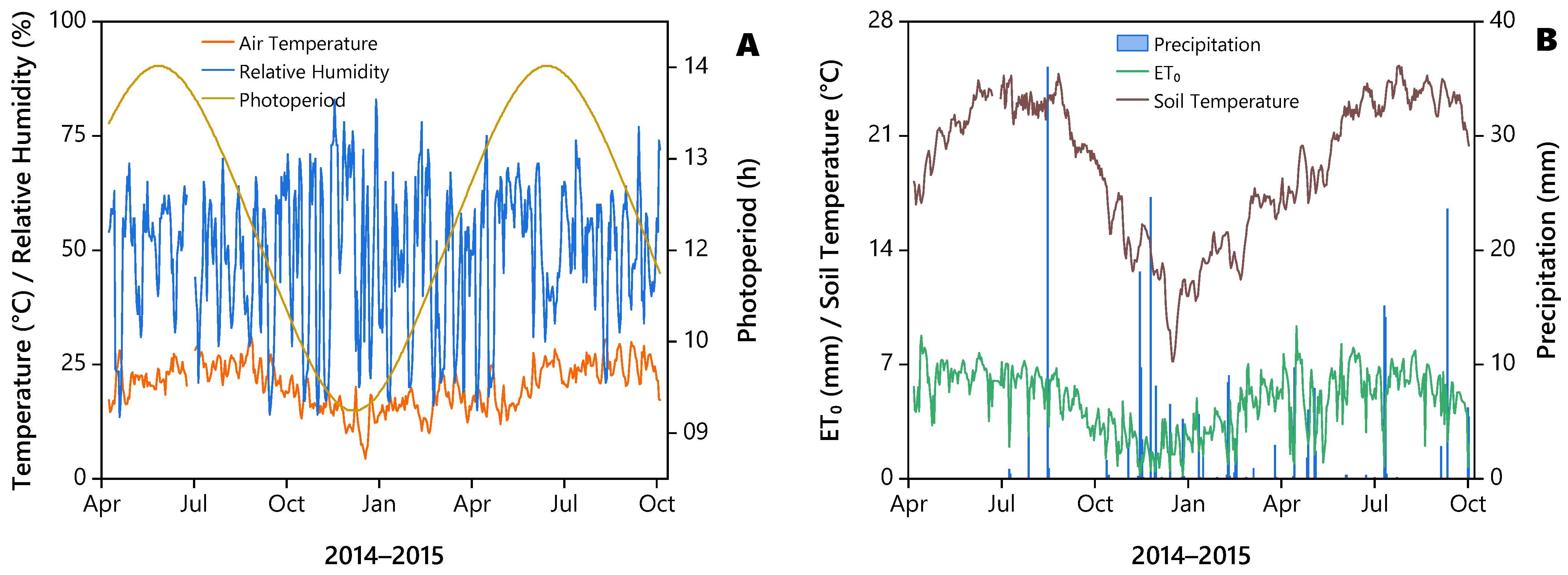
Figure 1. Environmental conditions during the year-long field experiment. (A) Average daily air temperature (°C), average relative humidity (%), and photoperiod (h). (B) Daily reference evapotranspiration (ET0, mm), average soil temperature (°C), and daily precipitation (mm). Source: CIMIS (California Irrigation Management Information System).
Agronomy 16 01283 g001
Figure 2. Percentage of green cover (PGC) evaluations of tall fescue as influenced by soil amendments during the establishment phase in 2014. Within each evaluation date, lowercase letters indicate soil amendment treatments that do not differ significantly according to the Scott–Knott test (p < 0.05). DAS, days after seeding.
Agronomy 16 01283 g002
Figure 3. Temporal dynamics of visual quality (VQ) in tall fescue as influenced by soil amendment treatments under 50% ET0 (A) and 85% ET0 (B) irrigation regimes across the 154-day evaluation period. The dashed red line indicates the minimum acceptable quality threshold (VQ = 6.0). Shaded ribbons represent ±1 SE (n = 4 replicates). Date-by-date treatment groupings (Scott–Knott, p < 0.05) are reported in Table S2. Treatment symbols and colors are defined in the legend.
Agronomy 16 01283 g003
Figure 4. Temporal dynamics of the normalized difference vegetation index (NDVI) in tall fescue in response to soil amendment treatments under 50% ET0 (A) and 85% ET0 (B) irrigation regimes across the 154-day evaluation period. Shaded ribbons represent ±1 SE (n = 4 replicates). Date-by-date treatment groupings (Scott–Knott, p < 0.05) are reported in Table S4. Treatment symbols and colors are defined in the legend.
Agronomy 16 01283 g004
Figure 5. Temporal dynamics of the dark green color index (DGCI) in tall fescue in response to soil amendment treatments under 50% ET0 (A) and 85% ET0 (B) irrigation regimes from 14 to 140 days after initiation (DAI). Shaded ribbons represent ±1 SE (n = 4 replicates). Date-by-date treatment groupings (Scott–Knott, p < 0.05) are reported in Table S6. Treatment symbols and colors are defined in the legend.
Agronomy 16 01283 g005
Figure 6. Temporal dynamics of soil volumetric water content (θv, %) under tall fescue in response to soil amendment treatments under 50% ET0 (A) and 85% ET0 (B) irrigation regimes across the 154-day evaluation period. Shaded ribbons represent ±1 SE (n = 4 replicates). Date-by-date treatment groupings (Scott–Knott, p < 0.05) are reported in Table S7. Treatment symbols and colors are defined in the legend.
Agronomy 16 01283 g006
Figure 7. Root morphology and architecture of tall fescue across soil amendment treatments under 50% ET0 (A) and 85% ET0 (B) irrigation regimes, within the upper 12 cm of the soil profile. Cell color encodes the treatment mean (n = 4) for each metric, standardized (z-score) within that metric across both regimes, so the ten metrics share a common scale; red indicates values above the metric average and blue below. Uppercase letters denote Scott–Knott groupings among amendments within each regime and metric (p < 0.05); within a column, cells sharing a letter do not differ. Treatment means, standard errors, and full statistics are reported in Table S8.
Agronomy 16 01283 g007
Table 1. Area under the progress curve (AUPC) of tall fescue visual quality as influenced by soil amendment and irrigation regime across the 154-day evaluation period (DAI 0–154).
Amendment50% ET085% ET0Amendment Mean
Untreated Control817.2 ± 72.91020.2 ± 30.7918.8 a
2.47 t ha−1 biochar876.8 ± 42.7978.2 ± 50.3927.5 a
12.36 t ha−1 biochar834.8 ± 41.11016.8 ± 50.3925.8 a
24.71 t ha−1 biochar890.8 ± 63.8973.0 ± 52.6931.9 a
5 cm biosolids736.8 ± 30.3819.0 ± 42.1777.9 b
5 cm greenwaste773.5 ± 60.91018.5 ± 18.2896.0 a
5 cm greenwaste + 12.36 t ha−1 biochar792.8 ± 37.5948.5 ± 17.7870.6 a
10 cm greenwaste857.5 ± 64.11008.0 ± 19.2932.8 a
Values are means ± SE (n = 4). Because the amendment × irrigation interaction was not significant (p = 0.573), amendments are compared as a main effect pooled across both irrigation regimes (final column); different lowercase letters denote significant differences (Scott–Knott; p < 0.05). The irrigation main effect was significant, with AUPC higher under 85% than 50% ET0 (p = 0.010).
Table 2. Pearson product-moment correlation coefficients among visual quality (VQ), dark green color index (DGCI), normalized difference vegetation index (NDVI), and volumetric water content (VWC) across the full evaluation period (DAI 14–140, n = 640) and the stress period (DAI 70–140, n = 384).
ParameterVQDGCINDVIVWC
Full Evaluation Period (14–140 DAI)
VQ1.0000.460 ***0.775 ***0.217 ***
DGCI 1.0000.590 ***−0.218 ***
NDVI 1.000−0.073 ns
VWC 1.000
Stress Period (70–140 DAI)
VQ1.0000.141 **0.733 ***0.591 ***
DGCI 1.0000.368 ***−0.025 ns
NDVI 1.0000.495 ***
VWC 1.000
*** p < 0.001; ** p < 0.01; ns, not significant. Bold text denotes the table headings, the two evaluation-period subheadings, and the parameter labels; it does not indicate statistical significance.
Table 3. Soil nitrate (NO3–N), ammonium (NH4+–N), and total nitrogen (Total N) concentrations at varying depths under tall fescue as influenced by irrigation regime and soil amendment.
Depth
(cm)
Irrigation
Regimes
Soil Amendment Treatments
T1T2T3T4T5T6T7T8
NO3 (mg kg−1)
0–1550% ET04.76 aB4.40 aB2.84 aC3.88 aB6.33 aA1.45 aC1.26 aC1.10 aC
85% ET02.00 bB3.58 aA1.98 aB1.81 bB4.41 aA1.26 aB0.94 aB1.11 aB
15–3050% ET03.75 aB4.37 aB4.17 aB2.47 aC7.46 aA1.29 aC1.43 aC1.02 aC
85% ET01.96 aA1.75 bA1.98 bA1.38 bA2.97 bA0.80 aA1.27 aA1.17 aA
NH4+ (mg kg−1)
0–1550% ET01.80 aA1.17 aB0.93 aB1.90 aA1.82 aA2.12 aA2.45 aA2.03 aA
85% ET01.17 aA0.68 aA1.22 aA0.66 bA1.09 bA1.70 aA0.89 bA1.62 aA
15–3050% ET00.88 aB1.71 aA1.25 aB0.90 aB2.16 aA1.76 aA1.64 aA1.83 aA
85% ET00.73 aA0.68 aA0.49 bA0.71 aA1.79 aA0.80 bA1.10 aA1.10 bA
Total N (mg kg−1)
0–1550% ET06.55 aB5.57 aB3.77 aC5.78 aB8.14 aA3.58 aC3.70 aC3.13 aC
85% ET03.18 bB4.27 aA3.20 aB2.47 bB5.50 aA2.97 aB1.83 bB2.73 aB
15–3050% ET04.63 aB6.08 aB5.43 aB3.37 aC9.62 aA3.05 aC3.06 aC2.84 aC
85% ET02.69 bB2.43 bB2.47 bB2.09 bB4.77 bA1.60 bB2.36 aB2.27 aB
Lowercase letters indicate statistically different irrigation regimes within each soil amendment treatment and depth, as determined by the t-test (p < 0.05). Uppercase letters indicate statistically different soil amendment treatments within each irrigation regime and depth, according to the Scott–Knott test (p < 0.05). Caption: (T1) untreated control, (T2) 2.47 t ha−1 biochar, (T3) 12.36 t ha−1 biochar, (T4) 24.71 t ha−1 biochar, (T5) 5 cm biosolids, (T6) 5 cm greenwaste, (T7) 5 cm greenwaste + 12.36 t ha−1 biochar, and (T8) 10 cm greenwaste. Bold text denotes the table headings and factor labels and does not indicate statistical significance.
Disclaimer/Publisher’s Note: The statements, opinions and data contained in all publications are solely those of the individual author(s) and contributor(s) and not of MDPI and/or the editor(s). MDPI and/or the editor(s) disclaim responsibility for any injury to people or property resulting from any ideas, methods, instructions or products referred to in the content.